the Creative Commons Attribution 4.0 License.
the Creative Commons Attribution 4.0 License.
 | 11 Mar 2022
Elements of future snowpack modeling – Part 1: A physical instability arising from the nonlinear coupling of transport and phase changes
Konstantin Schürholt
Julia Kowalski
The incorporation of vapor transport has become a key demand for snowpack modeling in which accompanied phase changes give rise to a new, nonlinear coupling in the heat and mass equations. This coupling has an impact on choosing efficient numerical schemes for 1D snowpack models which are naturally not designed to cope with mathematical particularities of arbitrary, nonlinear partial differential equations (PDEs). To explore this coupling we have implemented a stand-alone finite element solution of the coupled heat and mass equations in snow using the computing platform FEniCS. We focus on the nonlinear feedback of the ice phase exchanging mass with a diffusing vapor phase with concurrent heat transport in the absence of settling. We demonstrate that existing continuum-mechanical models derived through homogenization or mixture theory yield similar results for homogeneous snowpacks of constant density. When snow density varies significantly with depth, we show that phase changes in the presence of temperature gradients give rise to nonlinear advection of the ice phase amplifying existing density variations. Eventually, this advection triggers a wave instability in the continuity equations. This is traced back to the density dependence of the effective transport coefficients as revealed by a linear stability analysis of the nonlinear PDE system. The instability is an inherent feature of existing continuum models and predicts, as a side product, the formation of a low-density (mechanical) weak layer on the sublimating side of an ice crust. The wave instability constitutes a key challenge for a faithful treatment of solid–vapor mass conservation between layers, which is discussed in view of the underlying homogenization schemes and their numerical solutions.
- Article
(1736 KB) - Full-text XML
- Companion paper
- BibTeX
- EndNote


Neglecting vapor transport in the pore space of a snowpack for the overall mass balance is considered as a serious uncertainty in snow modeling. Persistent temperature gradients throughout the season may contribute to the depletion of snow density at the bottom of the snowpack due to upward vapor fluxes, as has been hypothesized for shallow tundra snowpacks by Barrere et al. (2017) and Domine et al. (2016). This problem is relevant for applications, for example, in permafrost where temperature gradients may induce the drying of soils with a feedback on snow metamorphism in the adjacent bottom layer (Domine et al., 2016), in turn affecting the ground thermal regime. Other applications of vapor transport comprise post-depositional redistribution of stable water isotopes in polar snow (Touzeau et al., 2018), density variations in polar firn (Li and Zwally, 2004), or the general impact on stratigraphy and metamorphism (Sturm and Benson, 1997).
The governing equations of macroscopic vapor transport in snow have been used for a long time. The homogenized equations of heat and purely diffusive vapor transport including phase changes have been derived from mixture theory in early work (Adams and Brown, 1990; Morland et al., 1990; Bader and Weilenmann, 1992). More recently, the equations were re-derived from a rigorous two-scale expansion (Calonne et al., 2014) yielding the same form of the resulting equations. The asset of the latter approach is the parameter control, which allows us to assess the model's scope and limits of applicability from the scale analysis. This homogenization method was later generalized to include effects of thermal convection (Calonne et al., 2014). Hansen and Foslien (2015) revisited the problem of coupled heat and vapor transport using mixture theory, leading to a more restrictive set of transport equations. They rely on the assumption that the vapor concentration is always close but not exactly in equilibrium with temperature. While the existing vapor schemes largely differ in the form of the effective transport coefficients, there is a general agreement on the basic type and form of the partial differential equations (PDEs) governing coupled heat and diffusive vapor transport in snow. These PDEs are coupled, nonlinear reaction diffusion equations. The diffusion terms are characterized by the effective diffusion constant and effective thermal conductivity in snow, while the reaction (or source) terms describe the phase changes, i.e., the volume-averaged, solid–vapor re-crystallization rates from metamorphism (Krol and Löwe, 2018). However, Calonne et al. (2014) and Hansen and Foslien (2015) both neglect the feedback of phase changes through an evolving ice phase in their numerical experiments. It is this coupling that needs to be understood for the incorporation of published homogenized vapor schemes into snowpack models for assessing the impact on snow density.
Recently Jafari et al. (2020) equipped the model SNOWPACK with a vapor transport scheme in the form of a nonlinear reaction–diffusion equation. It is the first attempt to solve the vapor diffusion equation in a snowpack model. The numerical solution requires time steps of 1 min and mesh sizes of 1 mm to avoid ”numerical oscillations” that were observed, even within an implicit, unconditionally stable numerical scheme. ”Sawtooth effects” attributed to ”slight numerical errors” were already revealed in early numerical work on the coupling of ice, vapor and energy transport in snow (Adams and Brown, 1990), and likewise, the numerical solution in Hansen and Foslien (2015) shows oscillations if longer simulation runs are considered (Andy Hansen, personal communication, 2017). Numerical issues have also been reported for solid–liquid phase changes when incorporating water flow into SNOWPACK via the Richards equation, which were attributed to density inhomogeneities (Wever et al., 2014). Phase change processes on seasonal timescales in polar snowpacks are important for climate modeling ideally adequately simulated on coarse meshes with large time steps. Therefore, it is necessary to understand the mathematical complexity of phase changes coupled to the mass transport equation. This will enable us to either design stable and accurate numerical schemes or otherwise accept simplified treatments which, in the case of vapor transport, could be, for example, based on a strict equilibrium assumption (Li and Zwally, 2004; Touzeau et al., 2018).
Due to the lack of analytical solutions for these nonlinear problems, confidence in orders of magnitudes of computed numbers can only be achieved via careful numerical experiments to address solver accuracy or mesh effects. This is naturally cumbersome within a full snowpack model. In addition, an explicit solution of the ice mass conservation equation is commonly avoided by using the Lagrangian frame of reference of the settling equation (Brun et al., 1989; Lehning et al., 2002). This complicates the assessment of phase change models in their originally published Eulerian form. Stand-alone numerical investigations of specific model components are therefore justified and necessary to understand nonlinear effects and numerical requirements for the design of efficient solvers in future snowpack models.
It is the aim of the present paper to advance the understanding of coupled heat and mass transport in snow by a careful numerical analysis of existing homogenization schemes. To overcome the limited flexibility in existing snowpack models we have implemented a stand-alone solver for the PDEs using the finite element (FE) framework FEniCS (Alnæs et al., 2015). The python-based computing platform was previously used for other problems in cryospheric sciences (Cummings, 2016). We focus on the nonlinear feedback of heat and vapor transport on an evolving ice phase. We consider the simplest setting and neglect convection in the gas phase and settling in the solid phase to provide a sound reference for future extensions. The question of how these effects can be coupled to settling will be addressed in a companion paper (Simson et al., 2021). Our approach will reveal the rich mathematical complexity that is hidden in published models and will provide evidence that the origin of this complexity is the density dependence of the effective transport coefficients in the presence of phase changes. We will show that this coupling causes the formation of wave patterns in the ice volume fraction profile as a true mathematical feature of the nonlinear PDE system. This is confirmed by an analytical, linear stability analysis attributing the unstable behavior to the density dependence of the effective (heat and mass) diffusion coefficients. The results suggest that previously obtained oscillations in the numerical schemes (Adams and Brown, 1990; Jafari et al., 2020) are physical and not numerical artifacts. With this work we seek to contribute to an understanding of if and how these features should be taken into account in future work.
The paper is organized as follows. In Sect. 2 we state the governing partial differential equations from the homogenization schemes (Calonne et al., 2014; Hansen and Foslien, 2015). In Sect. 3 we outline the finite element solution of the weak formulation of the problem and its implementation in FEniCS. In Sect. 4 we first provide an intercomparison of the two models in their original test scenarios and the scenario of a thin “Gaussian crust” as a smooth density heterogeneity. In Sect. 5 we characterize the observed migration of the ice phase under vapor re-crystallization by comparing the full model with an approximate advection equation for the ice phase which is derived under simplified assumptions. In Sect. 6 we detail the wave patterns that emerge in the numerical solution of the Gaussian crust. The analysis of the mesh resolution, integration time step and the residuals indicates that the wave patterns are intrinsic features of the mathematical model and not numerical artifacts. This is confirmed by the linear stability analysis in Sect. 6.2. After a few sensitivity tests we will discuss practical consequences of our study for vapor transport modeling in snow models (Sect. 8) and provide summarizing conclusions.
As a theoretical starting point we focus on two recently published homogenized formulations for an evolving vapor phase, namely Calonne et al. (2014) and Hansen and Foslien (2015). Despite differences in their theoretical homogenization approach, asymptotic expansion (Calonne et al., 2014) and mixture theory (Hansen and Foslien, 2015), both models have a very similar mathematical structure that resembles the earlier work of Bader and Weilenmann (1992).
2.1 Vapor scheme from Calonne et al. (2014)
The two-scale expansion for (vapor) mass and energy (Calonne et al., 2014) leads to the following set of equations for the vapor density ρv and the temperature T:
Here ϕi is the ice volume fraction, Deff the effective diffusion coefficient, ρi the constant density of ice, s the surface area density per unit volume, the volume-averaged normal velocity of the ice–air interface indicating deposition or sublimation, (ρC)eff the effective volumetric heat capacity (times snow density), keff the effective thermal conductivity and L the latent heat of sublimation.
The surface area density s, reflecting the current state of the microstructure and principally evolving in time, is assumed to be constant here in accordance with Calonne et al. (2014).
The source term on the righthand side (r.h.s.) of the vapor Eq. (1) quantifies phase changes, i.e., the net condensation rate. This implies the form of the energy source term through latent heat. In the simplest setting (Calonne et al., 2014), the volume-averaged interface velocity is given by
where β is the inverse growth velocity and the saturation vapor density. Note that strongly depends on the temperature, indicating the temperature feedback on the vapor mass balance. In order to close the system of Eqs. (1)–(3), parametrizations for the effective PDE coefficients must be provided (see below in Sect. 2.3). The feedback of a spatiotemporally evolving ice phase ϕi(z,t) has not been considered in Calonne et al. (2014).
2.2 Vapor scheme from Hansen and Foslien (2015)
A similar coupling scheme of the vapor transport to the energy equation has been put forward in Hansen and Foslien (2015). Using the same notation as above, these equations can be written in the form
Here the r.h.s. of both equations is expressed in terms of the condensation rate c.
The comparison of both models reveals that the vapor mass balance of Hansen and Foslien (2015) (Eq. 4) can be obtained from the corresponding vapor mass balance of Calonne et al. (2014) (Eq. 1) using the following reasoning: the deviation of the vapor concentration δρv from its equilibrium value will be mostly small. This suggests the use of an ansatz in Eq. (1). Assuming further that δρv diffuses faster than it relaxes locally, the deviation from equilibrium is kept nonzero only in the reaction term, which then implies Eq. (4). Hansen and Foslien (2015) support this derivation with a (non-rigorous) scaling argument to avoid two conflicting equations for the temperature T.
Though both presented models are strikingly similar in structure, it should be emphasized that the system of Eqs. (1)–(3) is closed and can be solved for ρv and T using an arbitrary closure for the condensation rate. This is different for the system of Eqs. (4)–(5): due to the simplifying assumption outlined above, Hansen's model lacks an evolution equation for the (perturbed) vapor mass balance. Since both vapor mass balance (Eq. 4) and energy balance (Eq. 5) are actually formulated in terms of the temperature T, Hansen and Foslien (2015) proceeds by consolidating both equations into a single equation which eliminates the condensation rate.
The latter now poses a nonlinear yet closed PDE that can be solved for the evolving temperature. Back-substituting the resulting temperature into either Eq. (4) or Eq. (5) allows us to evaluate the condensation rate c, without the freedom remaining to impose yet another closure relation. An additional, important implication of the near-equilibrium assumption in Hansen and Foslien (2015) is the impossibility to impose arbitrary boundary conditions for the vapor phase. By construction of the model, the boundary conditions are Dirichlet values for the equilibrium vapor concentration consistent with the boundary temperatures. Similar to Calonne et al. (2014) the feedback of a spatiotemporally evolving ice-phase ϕi(z,t) is not considered in Hansen and Foslien (2015).
2.3 Parametrization of the PDE coefficients
Despite similarities in the forms of the PDEs, both models have used different parametrizations for the transport coefficients Deff, keff and (ρC)eff and . While the two-scale homogenization presented in Calonne et al. (2014) contains derived expressions for the effective properties in terms of the microstructure as a byproduct, mixture theory in Hansen and Foslien (2015) relies on independently postulated parametrizations. The implications of these differences are presently still under debate (Fourteau et al., 2021).
In general, there is a broad agreement that all effective parameters are primarily influenced by the density or ice volume fraction ϕi. The goal of the present paper is not an exhaustive intercomparison of different formulations of the parametrized coefficients in the analyzed snow pack models. We rather want to focus on the intrinsic features and physical implications of the underlying process models. We therefore aim to keep differences due to specific flavors of the coefficients at the minimal level. To this end we use the same parametrization for the equilibrium vapor pressure and the effective heat capacity in both models but use different parametrizations for the effective thermal conductivity and diffusion constant. In the following we refer to these PDE parametrizations as the Calonne parametrization and the Hansen parametrization. All coefficients are stated explicitly in Appendix A.
2.4 Feedback from an evolving ice phase
The consistent treatment of phase changes requires a dynamic ice phase that evolves through recrystallization alongside the vapor phase in a mass-conserving way. This was considered in neither Calonne et al. (2014) nor Hansen and Foslien (2015). To investigate the feedback of an evolving ice phase on the two models from above we supply Eqs. (1)–(3) and (4)–(5) with a dynamic ice mass conservation equation (Bader and Weilenmann, 1992; Krol and Löwe, 2018). In the absence of settling but in the presence of phase changes, the continuity equation reduces to an ordinary differential equation for each location in space,
to balance the source terms in the vapor equations above. In Calonne's model can be evaluated from the closure relation (Eq. 3), whereas Hansen's c has to be reconstructed from either Eq. (4) or Eq. (5) as outlined before.
We summarize all symbols and parameter values of the models in Table 1.
Table 1Symbols, defining equations and constants used in this study.

To minimize the coding overhead and focus on the physical problem while keeping access to advanced numerical adjustments, the coupled PDE model was implemented using the python-based finite element framework FEniCS (Alnæs et al., 2015). It provides a high-level programming interface for the solution of PDEs in their weak formulation, with capabilities for parallelization and cross-platform portability via docker images. FEniCS' flexibility arises from its interface to the Unified Form Language (UFL) (Alnæs et al., 2015) which supports an intuitive declaration of discrete FE formulations of variational problems.
Below we outline the spatial and temporal discretization for the weak formulation of both systems (Eqs. 1–3 and 4–5), and describe the solution strategy employed for the coupled PDEs.
3.1 Spatial discretization – standard Galerkin
The nonlinear PDE systems of interest can be rewritten in the form
where F(u) is a nonlinear differential operator, and u is the (vector valued) solution that comprises the unknown fields. Following a standard Galerkin approach, the PDE's weak formulation is obtained by multiplying F(u)=0 with test functions v and integrating over the domain. The Galerkin method approximates the solution as the sum over a discrete set of basis functions {vj}, i.e., . This procedure allows us to apply the differential operator to the test functions. The test functions have a small support in which the values are nonzero, which simplifies the integral evaluations significantly. By choosing the test functions v from the basis {vj}, the PDE system is reduced to finding the roots of a (nonlinear) algebraic system. This standard Galerkin procedure is, for example, detailed in Donea and Huerta (2003). The implementation in the open-source finite element software FEniCS is straightforward.
3.2 Temporal discretization – theta method
Time derivatives are approximated using the theta method, also known as Rothe's method (Donea and Huerta, 2003). For a PDE of the form
the discretization reads
where un denotes the state vector's solution at time tn. Note that for θ=0 and θ=1 this reduces to standard first-order explicit and implicit Euler methods, respectively, whereas for it constitutes a weighted average of both.
3.3 Coupling scheme
Due to the different timescales of the involved equations, a monolithically coupled solution for the vector would be most consistent, yet it turns out to be inefficient. The vapor equation has by far the fastest dynamics, followed by the second fastest, the energy equation. The ice mass balance equations have much slower dynamics. The water vapor and energy equations are coupled diffusion–reaction equations and directly determine the r.h.s. of all equations. Therefore we solve them together in a first step and subsequently integrate the ice equation with its expected slower dynamics in a separate step. This operator splitting allows an independent fine-tuning of the numerical methods. Practically, we included the r.h.s. of the equations as an algebraic constraint in the state vector, i.e., for Calonne and for Hansen, which are then solved in a fully coupled way. The ϕi-dependent coefficients of the vapor and energy equations use ϕi from the previous time step. Subsequently ϕi is updated via (or c). Time step size is mostly determined through the vapor and energy dynamics. Changes in ϕi, and hence in the PDE coefficients, are therefore expected to be very small, which justifies the splitting-based coupling procedure.
We apply different theta values for each differential operator. For the diffusion operators in the vapor and energy equations we use θ=0.5 (Crank–Nicolson) which is known to be stable and convergent with second-order accuracy for linear operators. As the phase change (source) terms are expected to be stiff, a fully implicit, unconditionally stable backwards Euler scheme with θ=1.0 is applied.
To evaluate the models, we tested them on three different scenarios comprising specific combinations of initial conditions (ICs) and boundary conditions (BCs). The first two scenarios discussed in Sect. 4.1 and 4.2 are taken from Calonne et al. (2014) and Hansen and Foslien (2015), respectively, while the last (Sect. 4.3) is the simulation of a Gaussian-shaped crust. The three scenarios test different relevant aspects of snow modeling, namely the transient response to time-dependent BCs, piecewise-linear ice profiles covering the entire range of snow densities and lastly a high-density layer in a small sample with smooth, high-density gradients. For each of the three physical scenarios, we evaluate three model formulations: first, Calonne's Eqs. (1), (2) and (7) with Calonne coefficient closure from Appendix A (referred to as Cal-Eq/Cal-Par); second, Hansen's Eqs. (6) and (7) with the Hansen coefficient closure from Appendix A (Han-Eq/Han-Par); and third, the mixed case of Hansen's Eqs. (A5) and (7) with Calonne coefficient closure (Han-Eq/Cal-Par).
4.1 Scenario 1: homogeneous snow – transient heating at the boundary
The first scenario is proposed by Calonne et al. (2014) and investigates the response of a homogeneous snow layer on transient heating. The initial conditions are
with T0=273 K and . We employ a fixed Dirichlet BC at z=0 and a transient temperature drop at , viz.
where the transient drop is characterized by the Heaviside step function Θ with parameters τ=5 h and TH=263 K.
The solutions of all three cases we obtain for this combination of IC and BC are shown in Fig. 1 for t=100 min. Notably, Calonne's and Hansen's model along with their own (different) parameterizations for the PDE coefficients deviate in all variables since Hansen's effective diffusion constant is higher. This difference does not depend on the underlying process models but is rather due to the formulations used of the PDE coefficients as shown by the mixed case (Han-Eq/Cal-Par) which coincides with Han-Eq/Han-Par. Only a small difference can be observed close to the right boundary, where the changes in T and ρv are the fastest, and therefore the assumption underlying Hansen and Foslien (2015) is violated.

Figure 1Comparison of Calonne's and Hansen's model for the response to a transient temperature decrease at the boundary without ice-phase evolution: slight differences are observed if the models are used with their own formulation of coefficients (red and green line), while both yield virtually indistinguishable results if the same coefficients are used (red and turquoise line).
4.2 Scenario 2: heterogeneous snow – fixed temperature boundary conditions
Next we investigate the test case envisaged by Hansen and Foslien (2015) that comprises a piece-wise linear density profile as an approximation for a layered snowpack containing a crust with an additional ice layer at the bottom to constrain the vapor from below. The IC is given by
with T0=273 K and TH=253 K. The BCs are given by
The corresponding simulation results are shown in Fig. 2 at a simulation time of 38 h. Again, the fields ρv and T highly agree in homogeneous regions as long as the same parameterizations for the PDE coefficients are used. In contrast, the phase change term (r.h.s. of the equations) shows an agreement only if the same equations are used. This is revealed in the kink regions of the profile where Han-Eq/Han-Par coincides with Han-Eq/Cal-Par. This shows the different sensitivities of the T, ρv and phase change terms on the form of the homogenized equation when density gradients are present.
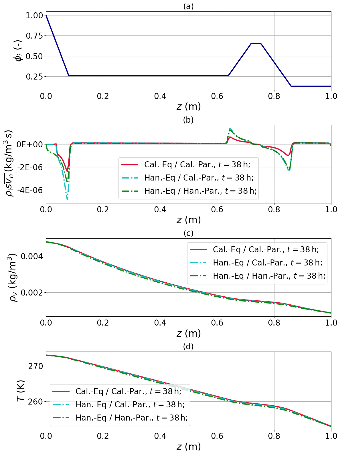
Figure 2Comparison of Calonne's and Hansen's model for the response to a piecewise-linear, layered profile under a temperature gradient without ice-phase evolution: the results for Hansen's model are indistinguishable even if different PDE coefficients are used (green and turquoise lines) but differ from the Calonne model (red line).
4.3 Scenario 3: the Gaussian crust
To further detail the response to high-gradient regions in the ice phase, our third scenario investigates the response of the models to a smooth, small-scale density variation under a temperature gradient in a shallow snow sample of height H=0.02 m. This scenario investigates the response of the models to density changes occurring on small length scales, e.g., layer interfaces which can be monitored in tomography experiments (Hammonds et al., 2015). In contrast to the previous two scenarios, the ice phase is now evolving according to Eq. (7).
In the following we solely focus on differences between Cal-Eq/Cal-Par and Han-Eq/Han-Par and investigate this difference at different physical times. We refer to this scenario as a Gaussian crust. As IC we employ
with T0=273 K, TH=253 K, , , z0=0.01 m and m2. For the Gaussian crust we use the same boundary conditions as in Eq. (17).
Figure 3 shows the simulation results for several points in time. Similar to before the solutions for ρv and T agree very well, and notable differences are observed for the phase changes in density transition regions. From this comparison for a smooth density variation, two additional observations can be made for both models. These are a consequence of the evolving ice phase.
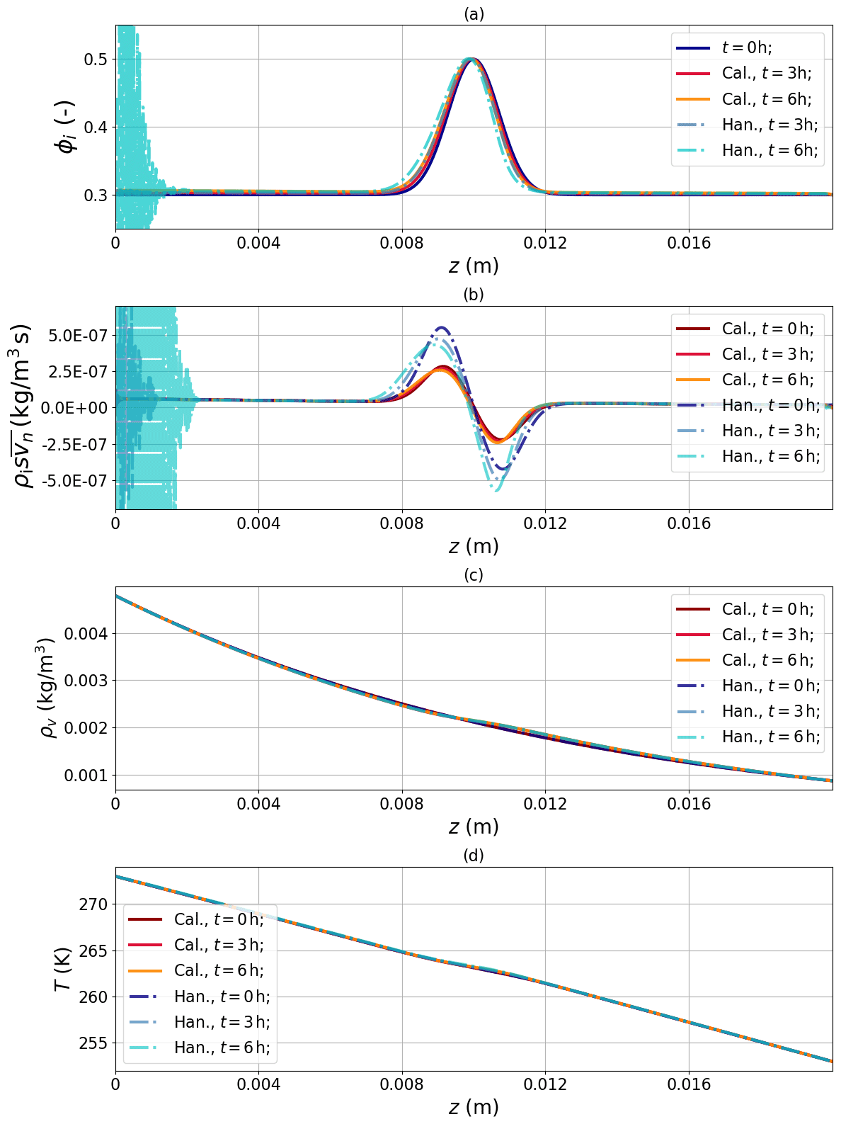
Figure 3Comparison of Calonne's and Hansen's model each with their own formulation of coefficients. Both models are coupled to the evolving ice phase for an initial Gaussian profile under a temperature gradient.
First, the Gaussian crust shows a quasi-advection in the ice phase towards the warm boundary despite the absence of an explicit advection term in the ice equation. During this quasi-advection, density gradients steepen on the cold side and flatten on the warm side. Far away from the crust a linear density gradient emerges in the domain as a consequence of the boundary conditions. The difference between the models lies in the apparent advection velocity. This is consistent with the observed differences in the phase changes since recrystallization rates differ approximately by a factor of 2.
Second, in both models oscillations emerge at the lower boundary. They are modest in the Calonne model and arise at a considerably later time with smaller magnitude. For the Hansen model these are apparent immediately.
These two observations are further detailed below.
The quasi-advection of density heterogeneities in the ice phase despite the absence of an explicit advection term in Eq. (7) is a consequence of phase changes (vapor sublimation and re-sublimation) as an intrinsic feature of the coupled system.
To understand the origin of this quasi-advection, we approach the coupled system (Eqs. 1, 2 and 7) with several analytical approximations. Justified by the separation of timescales we first restrict ourselves to stationary heat transfer and neglect the phase changes in the energy equation following arguments given in Calonne et al. (2014). This is a considerable simplification since the two-way coupling between heat and vapor is eliminated. Consequently, the heat equation ∇keff∇T=0 can be solved for the BC of Eq. 17 independent of the vapor transport process even for an inhomogeneous ice profile, with its exact solution given by
The local temperature (and its gradient) is thus a functional of the heterogeneous, non-constant ice volume fraction ϕi via the dependence of the effective conductivity keff on ϕi. We express this in the form
which defines the functional ℱT via Eq. (21). Motivated by the similarity between the solutions of Calonne et al. (2014) and Hansen and Foslien (2015) found in the previous section, we adopt the simplification from Hansen and Foslien (2015) and account for deviations in the vapor concentration from equilibrium only in the phase change (source) term. Again, we use a stationary diffusion equation due to the separation of timescales between vapor and ice. This allows us to rewrite the ice mass conservation Eq. (7) in a conservative form as a single advection equation,
with a functional,
that expanded by means of the chain rule and then uses the previously derived temperature expression (Eq. 22). The boundary conditions
follow from the BC of the vapor phase.
We stress the significance of this result. First, by using the approximations for the heat and vapor transfer, the three coupled heat and mass conservation equations can be equivalently cast into a single continuity equation for the ice phase. Second, the form of this continuity equation is a nonlinear and non-local advection equation, which explains the nature of this quasi-advection as a variant of shock formation reminiscent of the nonlinear Burgers equation (Du et al., 2012).
To test the derived approximation we have compared the numerical solution of Eq. (23) to the full solution of the Calonne model as shown in Fig. 4 for the Gaussian crust. In general, the agreement between the two models is very close, yielding almost identical results in homogeneous regions, i.e., towards the boundaries and close to the center of the crust. In the high gradient regions both models predict a steepening of the gradient, which is faster in the advection Eq. (23). Since Eq. (23) involves the same quasi-equilibrium approximation as used for the Hansen model, these quantitative differences are consistent with the results from the previous section.
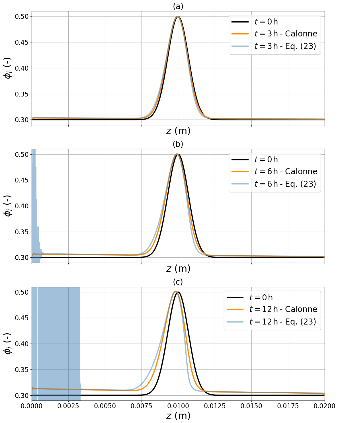
Figure 4Comparison between Calonne's model coupled to an evolving ice phase and the derived advection Eq. (23) for an initial Gaussian crust.
Despite remaining differences, the approximation (Eq. 23), together with Eq. (24), allows us to unambiguously trace back the quasi-advection and gradient steepening to the dependence of the effective diffusion constant and the effective thermal conductivity on ice volume fraction: if Deff was linear in ϕi and keff was constant, Eq. (21) would take the form of a simple advection equation, , with constant v. This would imply a shape invariant advection of any initial density profile. In contrast, the true Deff decreases and keff increases when the ice volume fraction is increased. Both dependencies lead to a decrease in the flux functional G in high-density regions, which explains the emergent asymmetry in the crust shape.
Similar to Eq. (3), the numerical solution of the advection equation also displays oscillations at the boundary already after a few hours. This will be further detailed in the following.
All numerical solutions so far are subject to oscillations at some point in time irrespective of the details. Therefore we will investigate the nature of these oscillations, now only considering the full Calonne model applied to the Gaussian crust.
6.1 Oscillatory solutions
The following example shows simulations with varying mesh size (number of elements ne) and varying time steps (dt) for the numerical solution at a fixed physical time. The results are shown in Fig. 5. Figure 5a shows the entire domain, revealing oscillations at the left boundary and on the sublimating side of the crust. Figure 5b shows a close up of the left boundary, while Fig. 5c shows a close-up of the sublimating side of the crust. For very low mesh resolution (ne=100, corresponding to a mesh size of 0.2 mm) and large time step (1 min), the solution in the vicinity of the crust oscillates from node to node, while for sufficiently high resolution the numerical solution converges to a smooth wave pattern independent of temporal and spatial resolution. This suggests that these waves are an intrinsic feature of the Calonne model equations rather than an artifact of the numerical scheme.
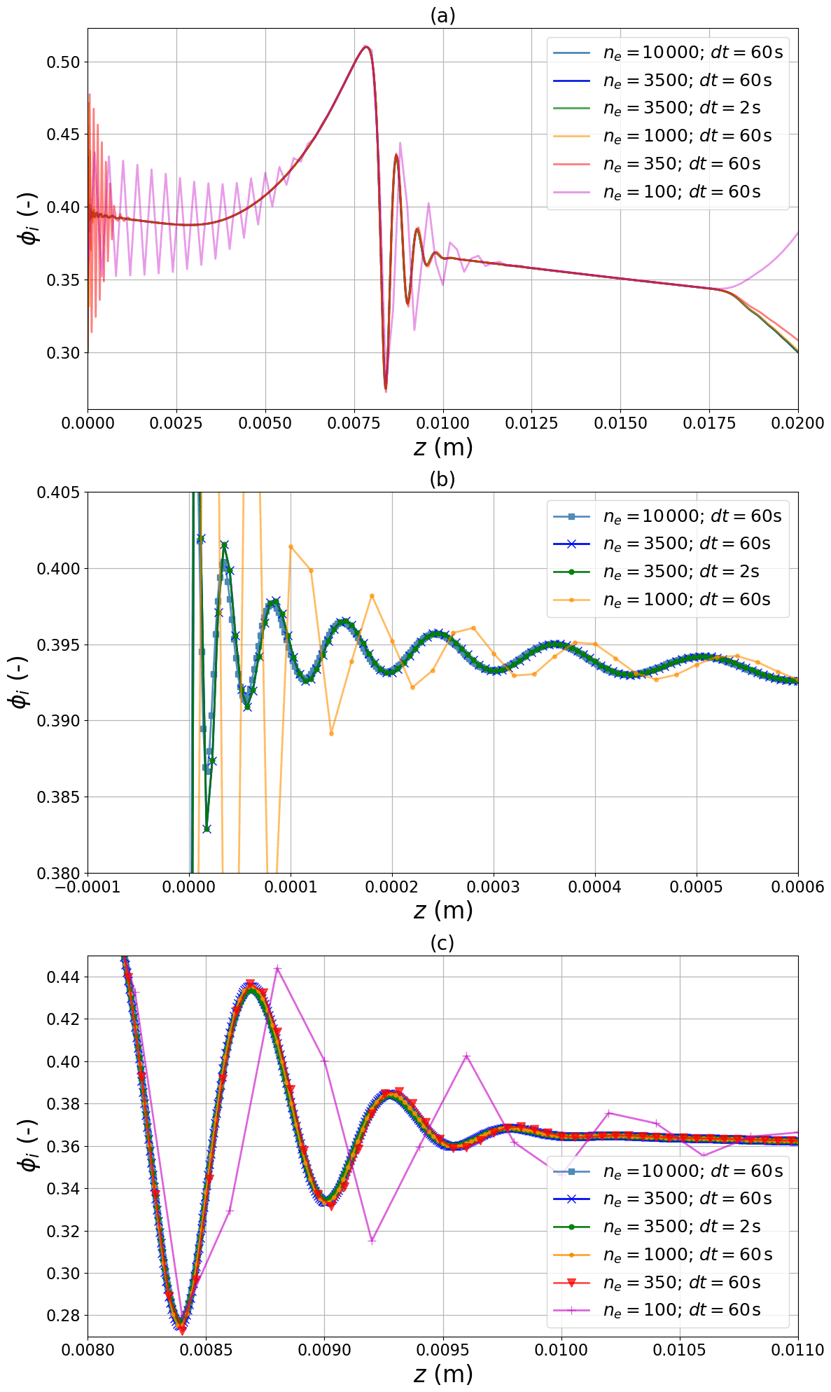
Figure 5Sensitivity of the numerical solution to mesh resolution and time step size: (a) entire domain, (b) close-up of the left boundary region and (c) close-up of the sublimating (right) side of the Gaussian crust. Apart from the coarsest resolution, the lines are almost indistinguishable, indicating numerical convergence to the true solution.
As an additional check we have analyzed the residuals of the numerical solution (see Appendix B) which confirms that patterns persist even when enforcing the residuals to approach zero.
6.2 Linear stability analysis
We use perturbation theory to further comprehend the oscillatory nature of the solution. Pattern formation in nonlinear PDE systems can be generally understood by investigating the dynamics of perturbations around a known stationary state via linear stability analysis of the dynamical equations. To do so, we start from the full, nonlinear, coupled, transient situation (Calonne model) in the form
which is only subject to the simplification that on the r.h.s. the division by ρeq(T) in Eq. (3) is subsumed in the prefactor α which is assumed to be constant.
The system (26) is, as before, equipped with Dirichlet BC for the two PDEs,
at the bottom z=0 and top z=H of the domain. To proceed analytically, we need to make an additional assumption to obtain an exact stationary solution of the system. We assume that the equilibrium vapor concentration is a linear function in T. This is reasonable within thin layers where temperature differences are small and a linearization of the equilibrium vapor curve is always justified. This linearization is written in the form
as an expansion around a reference temperature Tref (e.g., the mean temperature in the sample). With this assumption, a stationary solution of Eq. (26) can be obtained by inspection. It is easily verified that the system
satisfies Eq. (26) with BC Eq. (27) for arbitrary, constant volume fraction ϕi,0.
To carry out the stability analysis we use a vector notation and combine the fields in the vector . Then the PDE system (26) can be written in the matrix form
with state-dependent (3×3) matrices K(u),C(u), constant matrix R and constant vector f defined by
Then, the (stable) stationary state of Eq. (29) is denoted by the vector
The nonlinearities of Eq. (30) emerge from the dependence of the matrices K≡K(u) and C≡C(u) on u. Note that this dependence is solely through the third component of u (i.e., ϕi) which highlights the special role of the density (evolution).
Next we investigate the linear stability of the fixed point (32). To this end we make an ansatz,
and investigate the dynamics of the deviation from the stationary state u(0) by deriving an equation for u(1) through a perturbation expansion of Eq. (30) in first order. This procedure (carried out in detail in Appendix C) yields an equation for the Fourier modes of the perturbation for wave number k which can be written in the form
with a wave-number-dependent matrix,
with constant matrix coefficients K(0),V(0) and C(0). The eigenvalues of Mk control the behavior of the system in the vicinity of the stationary state. The matrix Mk is non-Hermitian due to the “advection” matrix V(0) and the “phase change” matrix R. Thus these two processes can principally cause eigenvalues with positive real parts (causing a growth of perturbations) and nonzero imaginary parts (causing oscillatory behavior). In the case of , Eq. (35) predicts negative eigenvalues for all k>0 and no pattern formation as it should be for simple diffusion equations.
The matrix Mk can be diagonalized in closed form using the symbolic algebra software MAPLE and eigenvalues subsequently separated into real and imaginary parts. Evaluating the eigenvalues with the corresponding parameter values from Table 1 shows that one of the eigenvalues has positive real part and nonzero imaginary part indicating a wave instability. This is controlled by the matrix V(0) with the coefficients k1 and D1 (see Eq. C12 in Appendix C) which characterize the sensitivity of the effective coefficients on density. Thus the instability originates from the fact that the effective diffusivity or the effective conductivity of snow depend on ice volume fraction (or snow density), and it is triggered by transitions in snow density, i.e., layers.
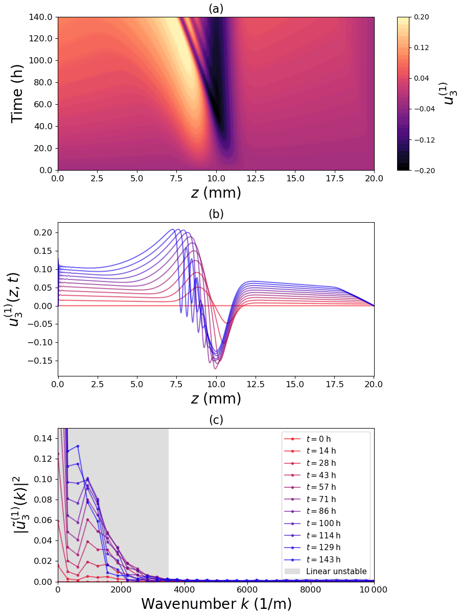
Figure 6Space–time plot of the perturbation field (a), profiles at different time steps (b) and corresponding power spectra (c).
We can compare the prediction of the stability analysis with the simulation of the full model for the Gaussian crust by analyzing the growth of amplitude of Fourier modes for wave number k through the power spectral density of the perturbation. To this end we have computed the third component of the perturbation vector as the deviation from the initial, oscillation-free state. The space–time plot of the perturbation in real space is shown in Fig. 6a which shows the emergence of the traveling wave. Discrete time steps are shown in Fig. 6b which displays the self-amplifying behavior of the density modulation in the layer-transition region, i.e., at the boundary of the crust. The power spectrum of the perturbation is computed via fast Fourier transform and shown in Fig. 6c as a function of wave number for different times, together with the theoretically predicted range of instability (eigenvalues with positive real part and nonzero imaginary part, gray region) derived from the diagonalization of the matrix Mk. The comparison confirms that growing modes are consistently lying in the unstable range. This supports our theoretical explanation that wave-like patterns emerge in regions of high-density gradients as an inherent feature of the coupled heat and mass transport in snow with density-dependent material properties.
Finally we conducted a few sensitivity studies to facilitate a discussion about the relevance of our findings in future snow modeling.
To confirm that observed wave patterns in the Gaussian crust are robust against variations of absolute values in temperature gradients and initial crust density, we simulated a denser Gaussian crust with different values for the temperature gradient. Figure 7a shows that the nonlinear PDE system essentially obeys time vs. temperature gradient scaling. Virtually the same wave solution is obtained at different physical times t which scale as . This test also shows that for a higher crust density, the density depletion on the sublimating side is more pronounced.
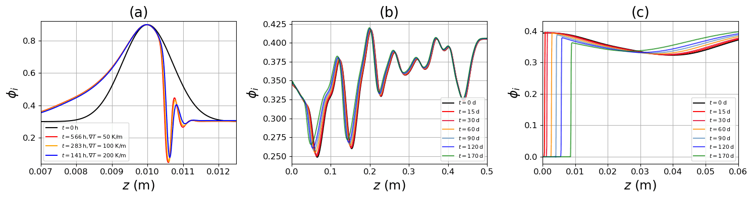
Figure 7Simulation of the fully coupled system: (a) time-temperature scaling. (b) Evolution of a smooth initial ice profile and fixed mean temperature gradient of 50 K m−1. (c) Same as (b) but with homogeneous Neumann BC and impact on depletion of mass at the boundary.
Second we subjected a smoothly varying density profile to a temperature gradient of 50 K m−1 and conducted a long simulation over 170 d. The results are shown in Fig. 7b. This confirms that if the density profile is sufficiently smooth, even an entire season simulation shows a stable, smooth advection of the ice phase.
Finally, we mimic the situation of a snowpack over a dry soil where no vapor can enter the system from below by imposing a zero-flux Neumann BC on the vapor equation. The results are shown in Fig. 7c indicating the order of magnitude of the expected depletion of the snow mass at the bottom for purely diffusive vapor transport under the influence of a temperature gradient of 50 K m−1 for an entire season.
8.1 Comparison of published homogenization schemes
We have revisited published models of coupled heat and (diffusive) vapor transport in snow. To investigate their numerical requirements we have implemented a stand-alone solver in the open-source software FEniCS for the sake of flexibility in numerical experiments involving spatial and temporal resolution, solution strategies, and accuracy.
From a mere physical point of view, our comparison of Calonne et al. (2014) and Hansen and Foslien (2015) has shown that both schemes yield similar results as long as the same parametrizations are used as closure for the PDE coefficients. The impact of purely diffusive vapor transport on macroscopic density changes is rather small (Fig. 7), in agreement with Jafari et al. (2020). Accurate estimates will certainly rely on the choice for the parametrization of the transport coefficients which naturally cause differences in the results (Fig. 1). In homogeneous parts of the snowpack these differences are small, and larger differences can be expected at layer transition regions (Fig. 2) where phase changes sensitively react to the underlying homogenized process model equations.
For the present work, however, the precise numbers were of minor importance. The primary goal was an assessment of the nonlinearity that is contained in published vapor homogenization schemes and their numerical requirements in view of previously reported numerical issues (Jafari et al., 2020, Adams and Brown, 1990, and Hansen and Foslien, 2015). While we have certainly challenged the numerical scheme by predominantly exploring high-temperature and high-density gradients, the observed time–gradient scaling (Fig. 7) indicates that the underlying nonlinear mechanisms are generally robust against these details.
8.2 Oscillatory behavior in the numerical solution
We have discovered that both models (Calonne et al., 2014; Hansen and Foslien, 2015) exhibit oscillations in the numerical solution if they are dynamically coupled to an evolving ice phase (Eq. 7). From our analysis of different combinations of initial and boundary conditions (Sect. 4) we conclude that two types of oscillations can occur: node-to-node oscillations (indicating numerical problems) and smooth oscillations (features of the underlying equations)
In view of numerical problems, we have shown that the dynamic coupling of the ice phase to heat and mass transport is equivalent to an advection of the ice phase (Sect. 5). The nonlinear nature of this advection causes a self-amplified increase in density changes and layer transitions, imposing special requirements on mesh resolution, time stepping and potentially shock-capturing schemes (Shu and Osher, 1988) to avoid oscillations. The fact that node-to-node oscillations occur on the “outflow” boundary of the ice phase supports this. In most of our simulations we have imposed a Dirichlet boundary condition of the vapor phase which is strictly in equilibrium on the boundary. By virtue of Eq. (23) this implies that the snow density cannot change directly at the boundary, while in the interior of the domain the ice is piling up towards the boundary under the advection (Fig. 4). This is reminiscent of outflow boundaries in fluid dynamics for high local Péclet numbers (Donea and Huerta, 2003): the disagreement between the information transported through the domain from the cold boundary and the information prescribed on the warm boundary is numerically resolved by steep node-to-node oscillations (Fig. 3). Similar issues can arise whenever abrupt changes in the advection velocity cannot sufficiently be resolved on a given mesh, as in Fig. 5 in the middle of the domain. This interpretation of node-to-node oscillations is supported by the fact that oscillations can be completely suppressed on the lower boundary by choosing a boundary condition, , for the vapor equation, which implies a vanishing gradient for the ice profile at the boundary. Our tests indicated that node-to-node oscillations can be eliminated by choosing a high resolution in space and time. A more efficient approach might be the utilization of stabilization methods for which our approximation (Eq. 23) may serve to provide a local advection velocity of the ice phase which needs to be supplied, for example, to a streamline upwind Petrov–Galerkin stabilization scheme (Donea and Huerta, 2003).
After increasing mesh and time resolution to suppress numerical problems, the true solution converges to a smooth, traveling wave pattern (Figs. 5, 6). As confirmed by the theoretical analysis, these oscillations are true features of the nonlinear homogenization equations and are triggered by gradients in the density (Sect. 6.2). These patterns can only form when the ice equation is dynamically coupled to the heat and vapor equation in a mass-conserving way. At the boundary, these physical oscillations are triggered as a consequence of the Dirichlet boundary condition as explained above: the competition of a fixed value of ϕi directly on the boundary for z=0 (implication of the imposed boundary conditions on the vapor phase for Eq. 7) and the increase in ϕi in the interior of the domain gives rise to a transition layer at the boundary with a high-density gradient in the ice phase that triggers the instability according to the mechanism revealed in Sect. 6.2. This is again supported by the fact that the physical oscillations at the boundary can be suppressed by choosing the BC for the vapor equations such that the gradient in ice volume fraction vanishes. This behavior is reminiscent of the wave instability triggered by a Dirichlet boundary condition in a 1D nonlinear reaction–advection–diffusion system (Vidal-Henriquez et al., 2017) which travels upstream into the domain.
8.3 Weak layer formation by wave instability?
We have shown that spatial heterogeneities in the density and ice volume fraction can amplify under the coupled thermodynamic description in snow. This has been pointed out before (Adams and Brown, 1990). We have investigated this phenomenon within the idealized scenario of a Gaussian crust where density gradients self-amplify under the nonlinear advective dynamics with a subsequent instability and the emergence of wave patterns. The eigenvalues of the linearized PDE system in our linear stability analysis have revealed the mechanism: a non-homogeneous density paired with the density dependence of the effective diffusion coefficients triggers the instability. Pattern formation following an instability is ubiquitous in nonlinear (diffusion–reaction) PDEs (Cross and Hohenberg, 1993).
In the present case, the observed instability may have far-reaching consequences, which comes as a (surprising) side-product of our numerical study: as the instability causes the depletion of density on the sublimating side of a crust (Fig. 7a), it explains why a low-density (mechanically weak) layer can form under these conditions. For high-density crusts, the parameters and model components used here predict a considerable reduction in the density in a sub-millimeter layer above the crust (Fig. 7a). This mechanism is solely a consequence of the continuum description of snow. We stress that this is different from a previously suggested reasoning (Colbeck and Jamieson, 2001), and it may occur as a superimposed effect on additional microstructural controls through near-crust metamorphism (Hammonds et al., 2015). In the future, it will be therefore important to assess how this instability is affected by adding mechanical settling, an evolving microstructure or enhanced mass transport from convection.
8.4 Open questions
8.4.1 Limits of the homogenization scheme
The present work poses questions on the limits of validity of the homogenization schemes used that are relevant for a user of the equations.
First, as detailed in Calonne et al. (2014), the homogenized Eqs. (1) and (2) are not valid for arbitrary growth rates. This is a tricky situation since the PDE system exhibits self-propelled dynamics into a state of fast growth for high-density gradients, thereby leaving its own range of validity. However, since the homogenization scheme (Calonne et al., 2014) does not contain the ice phase, it remains unclear if the equations used remain valid if a dynamical ice phase were included in the first place.
Second, the two-scale homogenization (Calonne et al., 2014) states assumptions on length scales, on which the description is meant to be valid. The expansion dictates what can be considered as homogenous: macroscopic scale which is sufficiently large against the microstructural length scale. But what happens if the derived equations contain mathematical features on smaller scales which violate the separation of scales? We have shown that the wave instability produces patterns on millimeter to sub-millimeter scales requiring ridiculously small mesh sizes to resolve them, clearly interfering with characteristic length scales of the microstructure. What is a consistent way of dealing with this situation? Resolving them numerically and averaging them out? Suppressing them numerically by artificial diffusion? Or does this behavior signal true multi-scale effects where the assumed “separation of scales” fundamentally breaks down? Answering these questions appears to be a key demand for future work on homogenization to provide a robust recipe on how to use derived equations correctly for applied modeling.
8.4.2 Discontinuous vs. continuous description of a stratified snowpack
Any snowpack contains variations in its properties that may be described either by continuous profiles containing large gradients (as done here) or by a discontinuous stacking of layers. We want to point out here that if a continuous description of density variations were to be replaced by discontinuous layers, the investigated wave problem will not simply disappear. In a hypothetical discontinuous layer description, as commonly pursued in snowpack models, the mass continuity of the ice phase at the layer interface would require us to derive a dynamic (nonlinear) equation for the migration of the layer interface on which the continuity of temperature and heat and mass fluxes were to be imposed. From the continuous description used here, no firm conclusion can be drawn on the behavior of the interface evolution between discontinuous, homogeneous layers. We hypothesize though that the wave instability of the continuous PDE formulation may translate into an oscillatory instability for the position of the interface. In view of the mathematical overhead of tracking continuity conditions at moving interfaces, we tend to recommend a continuous description in future snow modeling with numerical schemes that cope with arbitrary gradients in the properties.
8.5 Advantages and disadvantages of the numerical framework
We have used FEniCS for the stand-alone implementation to minimize the finite element method implementation effort while retaining full control of the numerical solution. Overall FEniCS provides a convenient, modular setup for exchanging PDE coefficients (keff,Deff) or boundary conditions, e.g., for more sophisticated exchange of vapor with the soil or the atmosphere. Alongside our study, we evaluated the FEniCS framework by comparing numerically different implementations. These experiences are shared for future reference.
We found that integration by parts in the weak formulation is not only necessary to apply Neumann boundary conditions but also increases the precision, regardless of the order of interpolation polynomials. Operator splitting turned out to be of limited value, the decrease in precision was not outweighed by a decrease in numerical complexity. As expected, a non-dimensionalization of the equations and the corresponding re-scaling to values of order unity did not impact the solution, as long as solver convergence settings are adapted. Increasing the polynomial order of the test functions was equivalent to increasing the mesh resolution with the corresponding number of nodes. However, we experienced large errors if the polynomial order of the variables of the coupled equations was not the same: solving ϕi in first order and ρv and T in second order caused large errors in the entire domain and also violation of the Dirichlet boundary condition. Adding auxiliary algebraic variables (as done here for the source terms) can improve the solvability of the system when convergence settings of the coupled system are adapted. Using so-called sub-functions in the formulation of the variational problem for coding modularity can introduce errors. We encountered deviations between a sub-function value and its hard-coded counterpart.
While FEniCS has provided an excellent numerical framework for the present study, a clear drawback of FEniCS would however emerge if mechanical settling was to be considered as a necessary, future extension. In the presence of settling, the ice-phase conservation equation is an advection-dominated problem which is notoriously difficult to solve on a Eulerian FE mesh without numerical smoothing. Re-meshing is currently not supported in FEniCS. To this end we have explored another, fully different numerical route to enable a flexible coupling of transport and phase changes to mechanical settling which is presented in Part 2 of this companion paper (Simson et al., 2021).
We have shown that the widely accepted form of homogenized vapor transport equations in snow predicts mathematical features (density waves) with interesting physical implications (weak layers) which constitute a considerable numerical challenge for future snowpack modeling.
Combining numerical experiments with theoretical considerations we have shown that the wave instability originates from the dependence of the effective heat and vapor diffusion coefficients (keff, Deff) on snow density. Since this dependence is the most fundamental nonlinearity in coupled heat and vapor transport in snow, it is unlikely that this effect will luckily disappear when considering more complex, nonlinear extensions of the model. The instability is a true feature of published equations and comes into play when the ice phase is dynamically coupled to the vapor phase by phase changes in a mass-conserving way.
The instability is triggered by high-density gradients which either (pre-)exist in snowpacks in the form of layers or are generated from the self-amplification of density gradients under the coupled dynamics. This amplification is a consequence of the effective advection of the ice phase due to phase changes. This is explained within the derivation of an approximate, nonlinear and non-local advection equation. Given the observed (approximate) equivalence between time and imposed temperature gradient, the system always undergoes a self-propelled evolution into its own instability. The instability might be practically irrelevant as long as smooth density profiles are considered. But the instability will certainly become relevant if a snowpack model should be applicable to simulate a sublimating side of a crust as a potential origin of weak layer formation.
We have outlined open questions and limitations of the present study related to the homogenization scheme, the numerical scheme and the concept of discontinuous layers. While the present study required a stand-alone numerical implementation, it seems to be of key importance that future snow models will be flexible enough for conducting advanced numerical studies. Only then will re-implementations of stand-alone numerical experiments become obsolete and the rich, nonlinear behavior of snow be able to be predicted from a snow model alone.
For the equilibrium vapor pressure we used the parametrization from Libbrecht (1999) given by
with Tm=273.15 K, Pa, Pa K−1, Pa K−2, Tr=6150 K, the conversion from pressure to density through the ideal gas law and J kg−1 K−1.
For the effective heat capacity we used a volume-averaged formulation given in Calonne et al. (2014):
with Ci, Ca and ρi given in Table 1.
In the Calonne case we used for the effective diffusion parameters Eq. (12) from Calonne et al. (2011) and the self-consistent estimate used in Calonne et al. (2014) given by
with k0=0.024, , and D0 given in Table 1.
In the Hansen case we used Eqs. (87) and (88) from Hansen and Foslien (2015) given by
and and D0 given in Table 1.
Due to the lack of an analytical solution for the nonlinear problem, we used the nodal residuals as an indicator for the solution error. FEniCS does not provide access to the nodal residuals to verify convergence in the NonlinearVariationalSolver
class. To this end we recovered the residuals manually by decoupling the equations and iterating over individually fine-tuned solvers for each equation. The results are
shown in Fig. B1. While in this solution scheme the residuals are several orders of magnitude smaller than in our regular setup, the onset of the wave instability remains the same (Fig. B2).

Figure B1Results upon lowering the residuals of all equations. While some pattern is still visible, the order of magnitude is small enough to assume small errors in the solution as well.
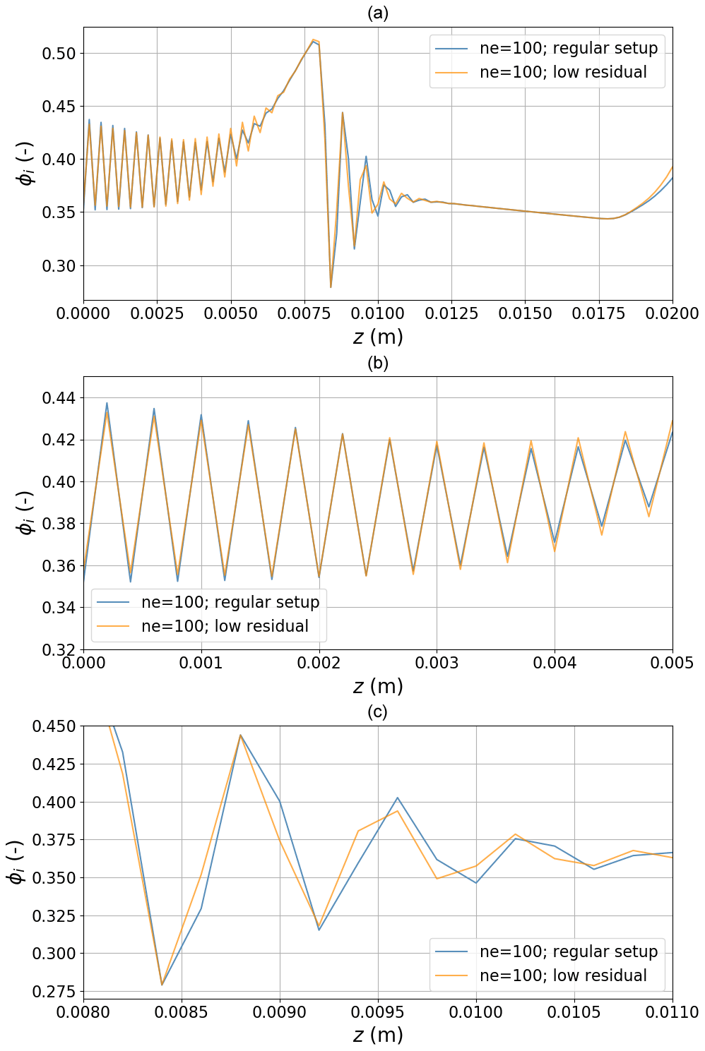
Figure B2Comparison between node-to-node oscillation patterns for the regular setup and the low-residual setup.
Carrying out the perturbation expansion of the PDE system (Eq. 30) around the stationary state (Eq. 31) using the ansatz (Eq. 33) requires two auxiliary relations which are stated below.
First, for any matrix M=M(u) that depends only on the third component u (ice volume fraction ϕi) the following holds:
where (⋅) denotes the scalar product on the 3D solution space.
Second, the expansion around the fixed point of an arbitrary matrix M=M(u) that depends only on the third component u (ice volume fraction ϕi) reads
where we use the following shorthand notation for the matrix coefficients:
Now we can state the expansion of the PDE system (Eq. 30) to first order in u as follows:
Equating zero- and first-order terms in u(0) provides an equation that is satisfied by the stationary state as it should be. By collecting terms linear in u(1) the governing equation reads
The advection term can be re-written in the form K(1)[∇zu(0)⊗e3]∇zu(1), and after multiplying the corresponding matrices we arrive at the final, linear PDE system with constant coefficients:
with coefficient matrices given by
In the latter step we employed the expansions of the diffusion coefficients around the reference volume fraction ϕi,0 in the form
Generally, it seems feasible (though tedious) to carry out an expansion of Eq. (C6) in a finite domain in terms of the eigenfunctions of the differential operator satisfying the BC. This would allow us to incorporate the impact of the BC into the stability analysis. Since u(0) already satisfies the original Dirichlet conditions, the perturbation u(1) must vanish on the boundaries. However, we limit ourselves here to the simpler case of a stability analysis in an infinite domain and take continuous Fourier transforms of Eq. (30) with respect to z. Denoting the Fourier variable by k we end up with the final result stated in Eq. (34)
The python FEniCS code for running all simulations and output analysis to reproduce the key Fig. 5 is available via https://doi.org/10.16904/envidat.298 (Schürholt et al., 2022).
The study was designed by HL and JK. Implementation, simulations and figures were done by KS with contributions and supervision from HL and JK. Derivation of the quasi-advection and the linear stability analysis was done by HL. The manuscript was written by HL with contributions from KS and JK.
The contact author has declared that neither they nor their co-authors have any competing interests.
Publisher's note: Copernicus Publications remains neutral with regard to jurisdictional claims in published maps and institutional affiliations.
We thank Andy Hansen for discussions and sharing his experience on his numerical implementation.
This paper was edited by Mark Flanner and reviewed by two anonymous referees.
Adams, E. E. and Brown, R. L.: A mixture theory for evaluating heat and mass transport processes in nonhomogeneous snow, Continuum Mech. Therm., 2, 31–63, https://doi.org/10.1007/BF01170954, 1990. a, b, c, d, e
Alnæs, M. S., Blechta, J., Hake, J., Johansson, A., Kehlet, B., Logg, A., Richardson, C., Ring, J., Rognes, M. E., and Wells, G. N.: The FEniCS Project Version 1.5, Archive of Numerical Software, 3, 9–23, https://doi.org/10.11588/ans.2015.100.20553, 2015. a, b, c
Bader, H. and Weilenmann, P.: Modeling temperature distribution, energy and mass flow in a (phase-changing) snowpack. I. Model and case studies, Cold Reg. Sci. Technol., 20, 157–181, 1992. a, b, c
Barrere, M., Domine, F., Decharme, B., Morin, S., Vionnet, V., and Lafaysse, M.: Evaluating the performance of coupled snow–soil models in SURFEXv8 to simulate the permafrost thermal regime at a high Arctic site, Geosci. Model Dev., 10, 3461–3479, https://doi.org/10.5194/gmd-10-3461-2017, 2017. a
Brun, E., Martin, E., Simon, V., Gendre, C., and Coleou, C.: An Energy and Mass Model of Snow Cover Suitable for Operational Avalanche Forecasting, J. Glaciol., 35, 333–342, https://doi.org/10.3189/S0022143000009254, 1989. a
Calonne, N., Flin, F., Morin, S., Lesaffre, B., du Roscoat, S. R., and Geindreau, C.: Numerical and experimental investigations of the effective thermal conductivity of snow, Geophys. Res. Lett., 38, L23501, https://doi.org/10.1029/2011GL049234, 2011. a
Calonne, N., Geindreau, C., and Flin, F.: Macroscopic modeling for heat and water vapor transfer in dry snow by homogenization, J. Phys. Chem. B, 118, 13393–13403, https://doi.org/10.1021/jp5052535, 2014. a, b, c, d, e, f, g, h, i, j, k, l, m, n, o, p, q, r, s, t, u, v, w, x, y
Colbeck, S. C. and Jamieson, J.: The formation of faceted layers above crusts, Cold Reg. Sci. Technol., 33, 247–252, https://doi.org/10.1016/S0165-232X(01)00045-3, 2001. a
Cross, M. C. and Hohenberg, P. C.: Pattern formation outside of equilibrium, Rev. Mod. Phys., 65, 851–1112, https://doi.org/10.1103/RevModPhys.65.851, 1993. a
Cummings, E. M.: Modeling the cryosphere with FEniCS, arXiv [preprint], arXiv:1609.02190, 9 September 2016. a
Domine, F., Barrere, M., and Sarrazin, D.: Seasonal evolution of the effective thermal conductivity of the snow and the soil in high Arctic herb tundra at Bylot Island, Canada, The Cryosphere, 10, 2573–2588, https://doi.org/10.5194/tc-10-2573-2016, 2016. a, b
Donea, J. and Huerta, A.: Finite element methods for flow problems, John Wiley & Sons, ISBN: 0-471-49666-9, 2003. a, b, c, d
Du, Q., Kamm, J. R., Lehoucq, R. B., and Parks, M. L.: A new approach for a nonlocal, nonlinear conservation law, SIAM J. Appl. Math., 72, 464–487, https://doi.org/10.1137/110833233, 2012. a
Fourteau, K., Domine, F., and Hagenmuller, P.: Macroscopic water vapor diffusion is not enhanced in snow, The Cryosphere, 15, 389–406, https://doi.org/10.5194/tc-15-389-2021, 2021. a
Hammonds, K., Lieb-Lappen, R., Baker, I., and Wang, X.: Investigating the thermophysical properties of the ice–snow interface under a controlled temperature gradient: Part I: Experiments & Observations, Cold Reg. Sci. Technol., 120, 157–167, https://doi.org/10.1016/j.coldregions.2015.09.006 2015. a, b
Hansen, A. C. and Foslien, W. E.: A macroscale mixture theory analysis of deposition and sublimation rates during heat and mass transfer in dry snow, The Cryosphere, 9, 1857–1878, https://doi.org/10.5194/tc-9-1857-2015, 2015. a, b, c, d, e, f, g, h, i, j, k, l, m, n, o, p, q, r, s, t, u, v, w
Jafari, M., Gouttevin, I., Couttet, M., Wever, N., Michel, A., Sharma, V., Rossmann, L., Maass, N., Nicolaus, M., and Lehning, M.: The Impact of Diffusive Water Vapor Transport on Snow Profiles in Deep and Shallow Snow Covers and on Sea Ice, Front. Earth Sci., 8, 249, https://doi.org/10.3389/feart.2020.00249, 2020. a, b, c, d
Krol, Q. and Löwe, H.: Upscaling ice crystal growth dynamics in snow: Rigorous modeling and comparison to 4D X-ray tomography data, Acta Mater., 151, 478–487, https://doi.org/10.1016/j.actamat.2018.03.010, 2018. a, b
Lehning, M., Bartelt, P., Brown, B., Fierz, C., and Satyawali, P.: A physical snowpack model for the Swiss avalanche warning: Part II. Snow microstructure, Cold Reg. Sci. Technol., 35, 147–167, https://doi.org/10.1016/S0165-232X(02)00073-3, 2002. a
Li, J. and Zwally, H. J.: Modeling the density variation in the shallow firn layer, Ann. Glaciol., 38, 309–313, https://doi.org/10.3189/172756404781814988, 2004. a, b
Libbrecht, K. G.: Physical properties of ice, SnowCrystals.com, http://www.cco.caltech.edu/~atomic/snowcrystals/ice/ice.htm (last access: 29 July 2021), 1999. a
Morland, L. W., Kelly, R. J., and Morris, E. M.: A mixture theory for a phase-changing snowpack, Cold Reg. Sci. Technol., 17, 271–285, https://doi.org/10.1016/S0165-232X(05)80006-0, 1990. a
Schürholt, K., Kowalski, J., and Löwe, H.: A numerical solver for heat and mass transport in snow based on FEniCS, EnviDat [code], https://doi.org/10.16904/envidat.298, 2022. a
Shu, C.-W. and Osher, S.: Efficient implementation of essentially non-oscillatory shock-capturing schemes, J. Comput. Phys., 77, 439–471, https://doi.org/10.1016/0021-9991(88)90177-5, 1988. a
Simson, A., Löwe, H., and Kowalski, J.: Elements of future snowpack modeling – Part 2: A modular and extendable Eulerian–Lagrangian numerical scheme for coupled transport, phase changes and settling processes, The Cryosphere, 15, 5423–5445, https://doi.org/10.5194/tc-15-5423-2021, 2021. a, b
Sturm, M. and Benson, C. S.: Vapor transport, grain growth and depth-hoar development in the subarctic snow, J. Glaciol., 43, 42–59, https://doi.org/10.3189/S0022143000002793, 1997. a
Touzeau, A., Landais, A., Morin, S., Arnaud, L., and Picard, G.: Numerical experiments on vapor diffusion in polar snow and firn and its impact on isotopes using the multi-layer energy balance model Crocus in SURFEX v8.0, Geosci. Model Dev., 11, 2393–2418, https://doi.org/10.5194/gmd-11-2393-2018, 2018. a, b
Vidal-Henriquez, E., Zykov, V., Bodenschatz, E., and Gholami, A.: Convective instability and boundary driven oscillations in a reaction-diffusion-advection model, Chaos, 27, 103110, https://doi.org/10.1063/1.4986153, 2017. a
Wever, N., Fierz, C., Mitterer, C., Hirashima, H., and Lehning, M.: Solving Richards Equation for snow improves snowpack meltwater runoff estimations in detailed multi-layer snowpack model, The Cryosphere, 8, 257–274, https://doi.org/10.5194/tc-8-257-2014, 2014. a
- Abstract
- Introduction
- Homogenized heat and mass transport
- Finite element solution in FEniCS
- Model comparison
- Quasi-advection of the ice phase
- Pattern formation
- Sensitivity studies
- Discussion
- Conclusions
- Appendix A: Parametrizations of the PDE coefficients
- Appendix B: Analysis of residuals
- Appendix C: Perturbation expansion of the heat–vapor–ice system
- Code and data availability
- Author contributions
- Competing interests
- Disclaimer
- Acknowledgements
- Review statement
- References