the Creative Commons Attribution 4.0 License.
the Creative Commons Attribution 4.0 License.
 | 25 Feb 2022
A comparison of the stability and performance of depth-integrated ice-dynamics solvers
Daniel Goldberg
William H. Lipscomb
In the last decade, the number of ice-sheet models has increased substantially, in line with the growth of the glaciological community. These models use solvers based on different approximations of ice dynamics. In particular, several depth-integrated dynamics solvers have emerged as fast solvers capable of resolving the relevant physics of ice sheets at the continental scale. However, the numerical stability of these schemes has not been studied systematically to evaluate their effectiveness in practice. Here we focus on three such solvers, the so-called Hybrid, L1L2-SIA and DIVA solvers, as well as the well-known SIA and SSA solvers as boundary cases. We investigate the numerical stability of these solvers as a function of grid resolution and the state of the ice sheet for an explicit time discretization scheme of the mass conservation step. Under simplified conditions with constant viscosity, the maximum stable time step of the Hybrid solver, like the SIA solver, has a quadratic dependence on grid resolution. In contrast, the DIVA solver has a maximum time step that is independent of resolution as the grid becomes increasingly refined, like the SSA solver. A simple 1D implementation of the L1L2-SIA solver indicates that it should behave similarly, but in practice, the complexity of its implementation appears to restrict its stability. In realistic simulations of the Greenland Ice Sheet with a nonlinear rheology, the DIVA and SSA solvers maintain superior numerical stability, while the SIA, Hybrid and L1L2-SIA solvers show markedly poorer performance. At a grid resolution of Δx=4 km, the DIVA solver runs approximately 20 times faster than the Hybrid and L1L2-SIA solvers as a result of a larger stable time step. Our analysis shows that as resolution increases, the ice-dynamics solver can act as a bottleneck to model performance. The DIVA solver emerges as a clear outlier in terms of both model performance and its representation of the ice-flow physics itself.
- Article
(2565 KB) - Full-text XML
-
Supplement
(97 KB) - BibTeX
- EndNote


Modeling ice sheets at the continental scale requires compromise. The Greenland and Antarctic ice sheets span hundreds to thousands of kilometers horizontally and interact with the rest of the Earth system on timescales of up to thousands of years. Solving the full Stokes stress balance at high resolution to calculate the ice dynamics over such a large domain for a long timescale is still computationally challenging. Therefore, it is important to reduce the complexity of simulations of ice dynamics.
Several factors reduce the need to simulate the whole system using the full Stokes equations. First, ice sheets typically have low aspect ratios, growing only a few kilometers thick near the domes but extending thousands of kilometers horizontally (i.e., ice sheets are shallow). This condition implies that over most length scales of interest, several terms in the stress balance can be ignored. Furthermore, some boundary conditions, particularly the basal friction at the bed, are poorly known, which means that the added accuracy in simulating velocities with a full Stokes approach may not translate into more robust estimates of past or future ice-sheet evolution.
Many approximations to the full Stokes stress balance exist, each with trade-offs. The simplest and historically most widely used shallow approximation is the shallow-ice approximation (SIA) (Hutter, 1983; Morland, 1984). The SIA is valid for slow-flowing grounded ice, frozen to the bedrock, which equates to shear flow induced by gravitational driving stress balanced by basal drag. It is a local solution, in that the velocity diagnosed at a given location is fully determined by the local driving stress. A complementary, but non-local, approximation is the shallow-shelf approximation (SSA) (Morland, 1987; MacAyeal, 1989), which represents fast-flowing ice that is either floating or sliding rapidly over the bed, resulting in plug flow (i.e., with a constant vertical profile of horizontal velocity).
An ad hoc approach to gaining the benefits of computational speed and validity in multiple flow regimes is to combine the SIA and SSA by summing their contributions to obtain the “hybrid” horizontal velocity field (hereafter called the Hybrid solver). This approach was proposed by Bueler (2009), who used a weighting function to transition between the two regimes. Later, Winkelmann et al. (2011) recognized that, in light of the approximations involved and the uncertainty in basal friction, it is more straightforward simply to sum the contributions. The fundamental assumption behind this approach is that the SSA represents a sliding regime, in which the depth-averaged velocity is equal to the basal velocity, while the SIA represents a frozen regime, in which the basal velocity is zero. In the former, it can be expected that SIA velocities will be negligible, and in the latter, SSA velocities will be zero. Only in the narrow transition between the two will the velocity solutions be mixed, and the Hybrid approach should provide a smooth transition. The Hybrid solver is used by several models today (e.g., Winkelmann et al., 2011; Pattyn, 2017; Quiquet et al., 2018; Robinson et al., 2020). In fact, roughly half the models participating in ISMIP6 Greenland and ISMIP6 Antarctica used a Hybrid solver (Goelzer et al., 2018; Seroussi et al., 2019; Goelzer et al., 2020; Seroussi et al., 2020).
Others have rigorously derived approximations based on variational principles that intrinsically account for both shear and stretching (Hindmarsh, 2004; Schoof and Hindmarsh, 2010; Goldberg, 2011). The depth-integrated approximations are especially appealing, since they are comparable in speed per time step to the SSA and Hybrid solvers. The depth-integrated solver derived by Schoof and Hindmarsh (2010) and formalized by Perego et al. (2012) is part of the L1L2 family of solvers, following the terminology of Hindmarsh (2004). We refer to it here as the L1L2-SIA solver. The stress balance is solved at one layer in the ice sheet – in this case, at the bed – while the effective viscosity accounts for stress arising from both shearing and stretching. Thus the solver enables a 2D solution of the system of partial differential equations (PDEs) and fast performance compared to 3D solvers. This solver naturally incorporates both shearing and sliding regimes while approximating the shear-stress components via the SIA, which facilitates its numerical solution. The L1L2-SIA solver is used by the BISICLES model (Cornford et al., 2013).
The so-called depth-integrated-viscosity approximation (DIVA) derived by Goldberg (2011) is also part of the L1L2 family of solvers. Here, the stress balance is formulated in terms of the depth-averaged velocity, but like the L1L2-SIA solver, the viscosity accounts for both shear and stretching. The shear stress, however, is not approximated, but the longitudinal and lateral stresses are treated as depth-independent, which facilitates a 2D solution of the system of PDEs. The viscosity is vertically averaged, and basal friction is cast in terms of the depth-averaged velocity. This solver has been used by continental-scale models to investigate dynamics and interactions with climate for the Greenland and Antarctic ice sheets (Arthern et al., 2015; Arthern and Williams, 2017; Lipscomb et al., 2019, 2021).
All the approximations described above have been used effectively in a variety of glaciological contexts, but there has been no rigorous, comparative study of their numerical performance. Until recently, the primary concern at the regional/continental scale has been to represent the physics of ice flow, i.e., ensuring that both sliding and shearing regimes are well represented – a motivation that contributed to the development of the Hybrid, L1L2-SIA and DIVA solvers. Today, however, the community is focused on running such simulations at high resolutions (i.e., Δx<5 km), as the tools and computational resources become available.
Given the importance of computational efficiency in modeling glacial dynamics at the continental scale, the goal of this paper is to investigate the numerical performance of the solvers described above, when coupled to mass conservation time stepping. We focus on the latter three solvers, which account for the dominant stress terms over most of an ice sheet, while the SIA and SSA solvers are useful boundary cases. Below, we first outline the numerical approach used by each of these solvers. Next, we derive stable time-step limits of ice thickness advection in an analytical test case for the DIVA and Hybrid solvers, with no analytical solution found for the L1L2-SIA solver. We investigate the underlying factors that can affect the maximum stable time step for each solver. The analytical results are also validated in idealized numerical tests. We then compare the performance of all five solvers in terms of stable time-step size and model computational speed in a realistic test case of quasi-steady-state simulations of the Greenland Ice Sheet. This is followed by a discussion of the results and conclusions.
We describe the assumptions and equations behind the five solvers considered here, namely the SIA, SSA, DIVA, Hybrid and L1L2-SIA solvers. These approximations can be obtained by considering the various terms in the first-order Blatter–Pattyn (BP) approximation (Blatter, 1995; Pattyn, 2003). To give context to the depth-integrated solvers, we first write the basic equations of the 3D BP stress-balance approximation:
where u and v are the components of horizontal velocity, μ is the effective viscosity, ρi is the density of ice (assumed constant), g is gravitational acceleration, s is the surface elevation, and are 3D Cartesian coordinates. In each equation the three terms on the left-hand side (LHS) describe gradients of longitudinal stress, lateral shear stress, and vertical shear stress, respectively, and the right-hand side (RHS) is the gravitational driving force. The longitudinal and lateral shear stresses together are also referred to as membrane stresses (Hindmarsh, 2006).
The effective viscosity μ is defined as
where A is the temperature-dependent rate factor in Glen's flow law (Glen, 1955), n is the Glen exponent (many models set n=3) and is the effective strain rate, given in the BP approximation by
Here, ux denotes the partial derivative , and similarly for other derivatives.
2.1 SIA solver
The shallow-ice approximation (SIA) solver is a zero-order approximation to ice flow that assumes a balance between the basal drag and the gravitational driving stress (Greve and Blatter, 2009). This leads to purely shear-stress-driven flow within the ice column. In other words, the membrane stress gradients are ignored, which leads to a stress-balance equation that can be solved locally. This is a typical flow regime for grounded ice that is not sliding.
By setting membrane stress gradients to zero in Eq. (1), we obtain the SIA stress-balance equations:
where the effective viscosity μ in Eq. (2) is obtained using an effective strain rate that includes only the shear terms:
Integrating Eq. (4) once, and by assuming a low aspect ratio and a free-stress surface boundary condition, we obtain
which can be integrated from the bed b to the height z to provide a 3D solution for horizontal ice flow:
The 2D vertically averaged velocity components and can then be obtained as
Equation (8) relies implicitly on the velocity solution via μ. In practice, an explicit formulation can also be found, which is more typical in model codes (e.g., Greve and Blatter, 2009). Furthermore, we note that the simplified case of uniform μ, Eqs. (7) and (8), can be integrated to give
It is possible to account for sliding in an SIA model, but Eqs. (7)–(9) apply to the regime where ice is frozen to the bedrock.
2.2 SSA solver
The shallow-shelf approximation (SSA) solver is complementary to the SIA solver in that the membrane stress gradients are retained, while the vertical-shear-stress gradients are ignored. This is a typical flow regime for floating ice or rapidly sliding ice streams, where the driving stress is low and the ice column has a uniform velocity profile (i.e., plug flow). By dropping the vertical-shear-stress gradient terms in Eq. (1) and integrating vertically while assuming a vertically uniform velocity, we obtain the 2D SSA stress-balance equations:
where τb,i indicates the basal stress in the direction i. For the SSA and subsequent approximations, we assume a basal-friction law of the form
where τb is the basal shear stress, is the basal velocity and β is a non-negative friction coefficient that can depend on ub. In the case of the SSA solver, . The effective viscosity is calculated following Eq. (2) for the BP solver, using a vertically averaged rate factor and computing the effective strain rate in 2D without the shear terms:
2.3 DIVA solver
Goldberg (2011) derived a higher-order stress approximation that is similar in accuracy to the first-order BP stress balance but like other depth-integrated solvers is computationally much cheaper. Since the stress-balance equations use a depth-integrated effective viscosity in place of a vertically varying viscosity, we refer to this scheme as a depth-integrated-viscosity approximation, or DIVA.
In the DIVA solver, the horizontal velocity gradients and effective viscosity in the membrane stress terms are replaced by vertical averages , and (Eq. 8). The 3D effective viscosity is given by Eq. (2) but with the DIVA effective strain rate:
The vertically integrated stress balance in DIVA can be written as
where the boundary conditions at b and s have been used to evaluate the vertical stress terms, and the basal stress is defined as for the SSA solver. Equation (14) has the same form as the SSA stress balance, but the dependence of basal stress and viscosity on velocity is more complex.
To solve Eq. (14) for the mean horizontal velocity components, the basal stress terms must be written in terms of and . The following discussion refers to the u component; the v component is analogous. Following Arthern et al. (2015), we define some generalized integrals ℱm for clarity:
Note that when n>1, these integrals depend implicitly on velocity through μ. Goldberg (2011) showed that the vertical profile of u is related to ub by
The surface velocity is thus related to the bed velocity as
Integrating u(z) from the bed to the surface gives the depth-averaged mean velocity :
which allows βub in Eq. (11) to be replaced with , where
For a frozen bed (ub=0, with nonzero basal stress τb,x), β will tend to infinity, whereby the above expression can be reduced to
To calculate the 3D viscosity field using the effective strain rate, Eq. (13), the vertical-shear-strain terms uz and vz must first be calculated, with uz (and similarly for vz) given by the expression (Lipscomb et al., 2019)
This expression depends on both τb,x and η, which can be obtained from the previous iteration.
The velocity is found in two steps. First, Eq. (14) is solved iteratively for the mean velocity, using Eqs. (11), (19) and (20) to write the basal stress terms in terms of and and Eqs. (13) and (21) to calculate the effective viscosity. Then Eq. (16) is integrated vertically to find the 3D velocity.
2.4 Hybrid solver
The Hybrid solver, as defined here, follows the approach of Winkelmann et al. (2011). The horizontal velocity is defined as the sum of the depth-dependent internal shear velocity (ui,vi) and the basal sliding velocity (ub,vb):
The sliding velocity is calculated via the SSA and the internal shear velocity is calculated via the SIA, as defined above. This approach generally works well because over most regions of an ice sheet, either plug flow (sliding) or shear flow is dominant, so one approximation is sufficient to represent the flow, and the other term goes to zero (Winkelmann et al., 2011; Pollard and DeConto, 2012). Although this approach is used widely with success at reproducing observed ice flow (e.g., Winkelmann et al., 2011; Quiquet et al., 2018), it is less clear how well it resolves the transition between the two regimes.
2.5 L1L2-SIA solver
The L1L2-SIA solver as defined here follows from Schoof and Hindmarsh (2010) and Perego et al. (2012). Like the DIVA and Hybrid balances, it is a two-step approach that begins by solving a depth-averaged stress balance. The balance is similar in form to the SSA, Eq. (10):
Aside from the fact that the equations are solved for basal, not depth-uniform, velocity, the balance differs from the SSA in the form of the effective viscosity. is a vertical average of μ′, the L1L2 effective viscosity, which is given by
where
with τb,ij, being the longitudinal stress induced by the basal strain-rate tensor. It should be noted that the form of μ′ is obtained by assuming that vertical shear stress can be approximated by the SIA solution (see Perego et al., 2012, for details). τb,e depends implicitly on , the effective horizontal (2D) strain rate induced by the basal strain-rate tensor (cf. Eq. 12):
For n=3, taking as a function of ub and vb from the previous iteration, Eq. (26) is a cubic equation for τb,e and can be solved analytically. Given from Eqs. (24) and (26), we can then solve Eq. (23) for ub and vb. Note that the trial viscosity μ′ makes the approximation that vertical shear stress is equal to the shallow-ice shear stress, −ρigH∇s. In the second step, three-dimensional vertical shear stress is diagnosed from the solution
where
τyz is diagnosed with a similar expression. Finally, we can define an updated viscosity:
Horizontal velocities are then given by
An important point regarding L1L2-SIA is the difference between μ′ and μ. The former is defined using the SIA shear stress as a proxy for the true vertical shear stress, while μ is formulated with an updated vertical shear stress based on the solution to the stress balance. This is in contrast to DIVA, where the viscosity is consistent between the two steps.
In this section, we assess the numerical stability of various schemes to solve the coupled stress-balance and continuity equations. Our analysis is closely related to von Neumann stability analysis (Isaacson and Keller, 2012), which has been developed for finite differences, but the non-local nature of the equations requires us to consider global solutions to the stress balance. For this analysis, we impose several simplifications.
-
We reduce the problem to one horizontal dimension by setting and ignoring the y derivatives.
-
We assume that the effective viscosity μ is spatially uniform. This is equivalent to assuming that the ice is isothermal with n=1 in Eq. (2) and the rate factor is constant, set to . This also implies that following Eq. (15).
-
We consider perturbations to an idealized geometry: an x-periodic domain with uniform thickness, H0, and surface slope, , where α>0.
This problem is described by Dukowicz (2012), who derived exact solutions for the velocity profile as a function of α and the non-dimensional parameter .
We specifically analyze the DIVA, Hybrid and L1L2-SIA solvers. We begin with DIVA, which leads to the simplest expressions for stability in this framework; results for the Hybrid balance follow. Finally, we attempt to analyze the L1L2-SIA balance but find that the complexity of the solver does not lend itself to an analytical result. The SSA analysis arises naturally, since the SSA equations have the same form as the DIVA solver. The numerical stability of an SIA solver under the above assumptions has been found previously (Hindmarsh, 2001; Cheng et al., 2017), showing that the maximum stable time step under the simplifications above is proportional to the square of the grid resolution:
We caution that the results depend on details of the numerical schemes and may not apply to all situations, such as when the rheology is nonlinear. Our aim is not to consider all possible schemes, or to produce a numerical scheme of optimal stability as in Cheng et al. (2017), but rather to examine stability properties when applying a representative finite-difference scheme to different stress-balance equations. As in Cheng et al. (2017) our analysis is applied to a linearized form of the coupled stress and continuity equations under small perturbations. Our analytical results provide context for the empirical time-step limits found in more realistic settings in Sect. 4 and give a theoretical basis for those results. Readers interested primarily in the performance of various depth-integrated stress balances in continental-scale ice-sheet models may wish to skip this section.
3.1 DIVA solver stability
We start with the x component of the DIVA stress balance, Eq. (14). By assuming a constant slope α and spatially uniform effective viscosity μ and by setting , this equation can be written as a second-order ordinary differential equation (ODE) for :
The first term on the LHS is the longitudinal stress, and the RHS is the driving stress. In the second term on the LHS, the quantity in parentheses is βeff, the effective basal-friction coefficient. This coefficient includes a non-dimensional parameter, , that relates basal friction to ice viscosity. If η is small, we have βeff≈β, and the flow is dominated by basal sliding. If η is large, then , and most of the flow is internal shearing. Note that in the context of this analysis, β is considered uniform.
To analyze the stability of a simple numerical scheme for the DIVA equations, we consider a reference state with uniform thickness H0 and surface slope α as described above. This reference state has uniform and hence zero longitudinal stress, with depth-mean velocity
The reference mean velocity can also be written as
where is the reference basal velocity. Following mass conservation, the thickness evolution equation can be written as a balance of horizontal flux divergence:
We will consider the evolution of thickness under a sinusoidal perturbation of the initial ice thickness:
Following Cheng et al. (2017), we substitute and in Eqs. (32) and (35), where is a perturbation in the mean velocity. Expanding terms and subtracting the zero-order balance, we can approximate the DIVA momentum–mass balance to first order in εh:
Next, we define a simple finite-difference scheme to solve this system of equations. While the theoretical domain has infinite extent, the computational domain must be finite, and we therefore consider a periodic domain of length L. The discretized perturbation thickness, hn, is located at points x=nΔx, for n=0, … ,N (where ), and the discretized perturbation velocity, un, lies at points , for n=0, … ,N−1. We assume that L is much larger than the parameter Lm, defined as
As shown in Eq. (A1), Lm is equivalent to a membrane stress length scale, over which longitudinal stresses are important (Hindmarsh, 2006).
Equation (37) is discretized as
where u is the vector of un; h is the vector of hn; hu is the vector of thickness hn averaged to u points; and Δn(⋅) indicates the first-order finite difference of a discrete function on the numerical grid, i.e., ). C is a symmetric, tridiagonal matrix with the entries
where
To proceed, an expression for in terms of δH and its derivatives is needed. For a linear stability analysis of SIA schemes (Hindmarsh, 2001; Cheng et al., 2017), this is straightforward, since velocity depends locally on thickness and surface slope. For the DIVA balance, however, a linear system (Eq. 40) must be solved. Analytical solutions to matrix equations are not always available, but for our assumptions (constant viscosity and flow in one horizontal direction) and geometry (periodic with constant surface slope and thickness), an asymptotically accurate closed-form solution can be derived. The mathematical details can be found in Appendices A1 and A2, but here we state the result:
where
The linearized mass balance equation, Eq. (38), is discretized with an explicit upwind scheme for the advective term and a centered difference for the divergence term:
With , and using Eq. (43) for um, this becomes
If the real part of the bracketed expression has an absolute value greater than 1 for an initial condition εheikx, this scheme is unstable.
Writing κ in full, the third term in brackets in Eq. (50) (i.e., the divergence term) can be written as
Defining θ≡kΔx, we seek the value of θ which maximizes the magnitude of the real part of Ξ. In doing so, we effectively ignore the second term in brackets in Eq. (51), which is purely imaginary. This is justified as we are primarily concerned with cases where Δx→0, where this term becomes negligible. In Sect. 3.4, however, we test the validity of the assumption over a wide range of Δx values. Using Eq. (45) to write in full, the remaining term is
This expression is non-positive, is continuously differentiable in θ, and has extremal points at θ=0 and θ=π. The maximum value occurs when :
We refer to the second term in brackets in Eq. (50) as γ. This term is related to advection and has a maximal value (when ) of
Together, γ and Ξ determine the stability of the time-stepping scheme. γ is related to advection, while Ξ arises from dynamic thinning and thickening under divergence. The presumption is that an arbitrary initial condition, unless carefully constructed, projects onto the mode eikx for which Eqs. (53) and/or (54) are realized. The scheme is stable when the real part of the bracketed expression in Eq. (50) has an absolute value less than 1 or, equivalently, when . When γ and Ξ are of similar magnitude, the associated limit on Δt does not have a simple expression. But when one or the other is dominant, there is differing leading-order behavior in the relationship between resolution and maximal stable time step. When γ≫Ξ, the equation system is essentially advective, and stability is governed by Eq. (54):
When Ξ≫γ, the maximum stable time step follows from Eq. (53):
The dependence of Δtdyn on Δx is more complex than that of Δtadv. It is useful, however, to consider two end-member regimes: large q and small q (in the following, it is assumed unless stated otherwise that Δtdyn≪Δtadv; i.e., advection is not a limiting factor). The case q≫1 corresponds to high basal friction and/or coarse resolution. In this limit it can be shown (see Eq. A1) that , so that , and Eq. (56) becomes
If η≫1, as in the case of high basal friction, this simplifies to
In this case, the stability criterion is identical to that of the SIA solver (Eq. 31), with the maximum stable time step, Δtmax, proportional to Δx2. This condition usually is not very restrictive for the DIVA solver, since large q typically implies coarse resolution if the ice is not too thin.
In contrast, for q≪1 (i.e., low basal friction and/or fine resolution), it can be shown that and . The terms in Eq. (56) containing a0 and r reduce to , resulting in
Thus, in the limit of small q (or equivalently, small Δx), the time-step limit arising from ice-flux divergence depends on μ and H0 but not Δx. This is not to say that the limiting time step is independent of resolution – but such dependence arises from the advective term, and thus the maximum stable time step varies linearly, not quadratically, with Δx. For a typical ice thickness of 103 m and effective viscosity of 106 Pa yr, we would have Δtdyn∼1 yr. With Δx=103 m and u0=103 m yr−1, the advective limit from Eq. (55) would also be ∼1 yr. At resolutions finer than ∼103 m, the maximum time step would be determined by the advective limit.
These two regimes of limiting time step correspond to differing behavior of the DIVA equations at different scales. In the large-q limit, Eq. (57), variations in velocity correlate closely with driving stress, and the dynamic response behaves like a diffusion process (similar to the SIA) in which the flux of thickness is proportional to thickness gradients, leading to a quadratic dependence of the limiting time step on resolution. In the small-q limit, Eq. (59), small-scale thickness oscillations are damped by dynamic thinning due to velocity divergence induced by the oscillations. The velocity gradients are scale-independent due to averaging of associated driving stresses over the membrane scale, resulting in a scale-independent damping rate and hence a scale-independent time-step limit, provided the advective time-step limit is large enough.
3.2 Hybrid solver stability
We consider now the Hybrid stress balance, in which sliding velocity is determined by the SSA momentum balance, Eq. (10). Thickness transport is due to a vertically averaged velocity , the sum of sliding velocity and the vertical average of the SIA velocity from Eq. (7), .
To investigate the Hybrid solver stability, we will first modify the DIVA analysis (Sect. 3.1) to treat the SSA case. Thus, we treat the SSA balance as a first step in the analysis of the Hybrid scheme. The SSA momentum balance (in one dimension, with constant viscosity) is
This is the low-friction limit of the DIVA balance, Eq. (32), with u replacing since velocity is depth-uniform. The SSA mass balance equation is given by Eq. (35), again replacing with u. The RHS of the matrix equation for velocity, Eq. (40), is identical, and the matrix C is modified with B=β. Thus, the dynamically limited time step Δtdyn is given by Eq. (56) but with r and a0 modified by the new definition of B. At high resolution, this leads to the same dynamically limited behavior as for DIVA, Eq. (59). At coarse resolution, the dynamically limited time step is similar in form but offset from DIVA due to the modified frictional term.
The Hybrid equations for momentum balance and mass conservation in 1D with constant viscosity μ are
where the mean shallow-ice velocity follows from Eq. (7). We consider the same reference state as in the DIVA analysis. The reference sliding velocity is
and the Hybrid depth-averaged velocity in this state is
Thus, , the DIVA depth-averaged reference velocity from Eq. (34). As before (cf. Eqs. 37 and 38), we consider perturbations in H of εheikx and write the equations to first order in εh:
where
Since , the Hybrid advective stability constraint is slightly more restrictive than for DIVA.
Consider the third term on the RHS of Eq. (66), which follows from the dependence of uSIA on perturbations in s. If this term is discretized using an explicit second-order finite difference, it can be expressed as
Note that this term is missing from the analogous equation for the DIVA solver, Eq. (38). With this result and those from the previous section (cf. Eq. 50 for DIVA), it can be shown that the limiting time step is determined by the constraint that
In the above expression, r and a0 are as defined as in Eqs. (46) and (47) but with the substitution B=β, giving . The third term of Eq. (69) is equal to as defined in Eq. (53) from the DIVA analysis. In the limit q≫1 (high basal friction and/or coarse resolution), this term reduces to
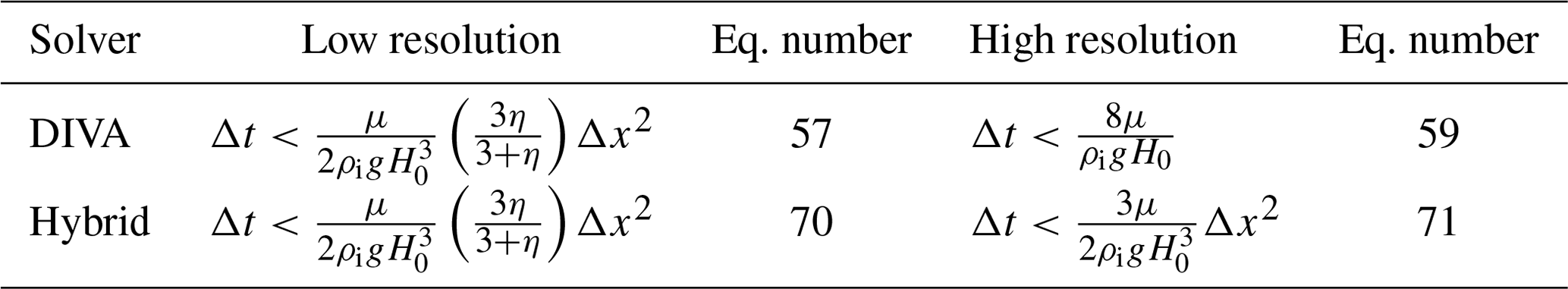
Table 1Summary of asymptotic time-step limits derived for the DIVA and Hybrid solvers under simplified conditions (1D, uniform viscosity, infinitely long ice slab of uniform thickness H0, explicit time-stepping scheme). An analytical solution was not found for the L1L2-SIA solver. Limits are shown for when the advective limit is sufficiently large so as not to apply and are defined loosely for low-resolution and high-resolution regimes. See the text for details.
Recalling that , the third and fourth terms can be combined to give
Provided the advective time-step limit is large, an approximate time-step limit in this regime is given by
which is identical to the large-q limit for DIVA, Eq. (57), and reduces to Eq. (58) when η≫1. When q≪1 (low basal friction and/or fine resolution), the third term in Eq. (69) is bounded independently of Δx (cf. the small-q limit Eq. 59 in the DIVA analysis). For small Δx, the time-step limit for small q is therefore governed by the fourth term:
Since Δt is proportional to Δx2, Eq. (71) becomes very restrictive at high resolution, like the identical equation for the SIA, Eq. (31).
In summary (see Table 1), both DIVA and the Hybrid solver have SIA-like stability (Eqs. 57 and 70) for large q (i.e., high friction and/or coarse resolution). However, in the small-q limit (low friction and/or fine resolution), the Hybrid scheme is governed by the SIA limit, Eq. (71), whereas DIVA is usually governed by a less restrictive advective limit, Eq. (55).
3.3 L1L2-SIA solver stability
In this section we attempt to analyze stability limits of the L1L2-SIA coupled stress–continuity equations. The complexity of the solver prevents us from deriving analytical expressions for time-step limits as with the other solvers, but we nonetheless comment on possible implications of the linearized expressions.
We first derive the expression for , the depth-integrated L1L2-SIA velocity, in the context of our simplified analysis (i.e., 1D flow with uniform viscosity). With these simplifications, Eq. (27) of Perego et al. (2012) for shear stress becomes
Integrating twice in z yields the depth-averaged velocity:
The stress balance which is solved for ub is identical to that of the Hybrid balance, and the reference velocity, , is identical to that of the Hybrid and DIVA balances. Linearizing the L1L2-SIA scheme around this state leads to a perturbed momentum balance identical to that of the Hybrid balance, and the perturbed mass balance is
The L1L2-SIA perturbed mass balance above has a similar form to those found for the DIVA and Hybrid cases but contains higher-order derivatives of δub. Treating these terms analytically as in Sects. 3.1 and 3.2 is beyond the scope of our study, and so we cannot give a rigorous stability bound in terms of resolution and governing parameters.
It is worth pointing out, however, that the second term in the parentheses in Eq. (74) gives rise to a second-derivative term (a diffusive term) in δH, which leads to the quadratic stability limit for small Δx in the Hybrid balance. In contrast to the Hybrid balance, this term is balanced by a term involving the second derivative of δub. Rearranging the linearized momentum balance, Eq. (65), yields
in which the LHS is equivalent to the terms in parentheses in Eq. (74). In other words, there is a degree of cancellation in Eq. (74), and this cancellation might lead to stabilization. While this argument does not provide a bound for stability, it suggests that the stability might be tied to the degree of cancellation of higher-order derivative terms in discretized form. Note also that, with a nonlinear rheology, the viscosity in Eq. (74) differs from that of the momentum balance (cf. Sect. 2.5), so that such cancellation will not occur for n>1, regardless of the numerical scheme.
3.4 Numerical validation
To confirm the validity of the stability bounds found in the above sections, we run numerical simulations with 1D DIVA, Hybrid and L1L2-SIA models derived using the assumptions above. Although we do not have an analytical expression to compare to for the L1L2-SIA solver, its numerical behavior can be compared to the other solvers. For the DIVA solver we use a first-order upwind finite-volume scheme for Eq. (35), and we use Eq. (32) for depth-averaged velocity. For the Hybrid solver, we use Eqs. (61) and (62), and for the L1L2-SIA solver, we use Eqs. (61), (73) and (35). The 1D code therefore implements the full coupled mass and momentum equations for DIVA, Hybrid and L1L2-SIA, rather than their linear perturbed forms. These simplified solvers have been implemented in MATLAB and are provided along with code to run the tests cases as a Supplement to the paper. As further validation, we run the same simulations using two comprehensive ice-sheet models, Yelmo (Robinson et al., 2020) and CISM (Lipscomb et al., 2019). The three solvers have been implemented in both models, and all test cases are simulated.
The test problem is solved with a periodic uniform slab as described in the beginning of this section, with the constant bedrock slope set to . For each model and parameter set, we verified that the diagnosed velocity profile (not shown) is consistent with the exact solutions.
To test stability, we add a random Gaussian perturbation to the initial ice thickness, such that
where 𝒳n represents independent Gaussian random variables with zero mean and standard deviation of 0.1 m. We then run the model forward for 100 time steps. While not guaranteed, it is likely that h(t=0) will project onto the least stable numerical mode (i.e., that for which the expressions defining Δtdyn and Δtadv are realized).
For a given set of physics parameters (), Δx is varied over a range from 10 m to 40 km (12 values are chosen, equidistant in log space – see the MATLAB code in the Supplement to reproduce the exact values). At each resolution we run multiple tests with different values of Δt to determine the maximum stable time step. For each run, we calculate the ratio , where σ is the standard deviation of h at the final time step, and σ0 is the standard deviation of h(t=0). The variance in ice thickness should decrease for a stable scheme, so this ratio serves as a metric of stability. We consider to indicate stability and to indicate instability. The numerical results are compared to the time-step limits determined analytically above.
We test two cases that are representative of different ice-flow regimes. The first parameter set ( Pa yr, H0=1000 m, β=1000 Pa yr m−1, η=10) corresponds to thicker, less viscous ice with a strong bed, i.e., conditions that favor vertical shear over sliding. In this case, u0 is equal to 39 m yr−1, and Lm is approximately 1.3 km. With such a low background velocity, the advective time-step limit Δtadv is not restrictive except at extremely high resolution, and so stability is determined by dynamic divergence alone. The second parameter set ( Pa yr, H0=500 m, β=30 Pa yr m−1, η=0.0375) corresponds to thinner, more viscous ice with a weak bed, i.e., conditions that favor fast sliding and vertically uniform flow. In this case, the maximum stable time step Δtdyn is generally larger (as a function of Δx) than in the thick, shearing case. Also, u0 is larger (150 m yr−1), which means that Δtadv may impose a stability limit as Δx becomes small. Figure 1 shows results for the two parameter sets from the simple 1D models and from Yelmo and CISM, as compared to the analytical solutions.
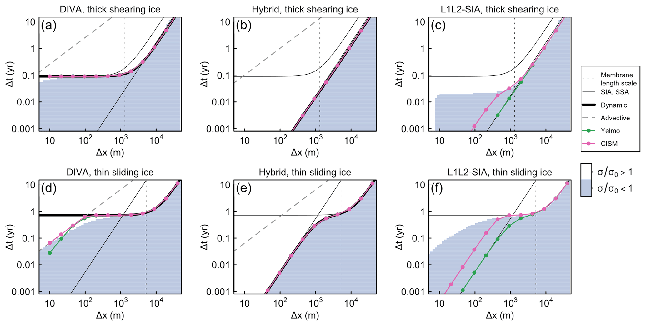
Figure 1Comparison of the stable time-stepping regime for the DIVA (a, d), Hybrid (b, e) and L1L2-SIA (c, f) solvers for a 1D slab of ice on a bedrock with constant slope () with thick shearing ice (a–c, H0=1000 m, Pa yr, β=1000 Pa yr m−1) and thin sliding ice (d–f, H0=500 m, Pa yr, β=30 Pa yr m−1). In all panels, the vertical thin dotted line indicates the membrane stress length scale Lm. For the DIVA and Hybrid solvers, the thin dashed grey line shows the advective time-step limit, Δtadv. For reference, the thin solid black lines show the analytical solutions for an SIA and SSA solver given by Eqs. (31) and (56) with B=β, respectively (the SIA solution is always depicted as a straight line). The thick black lines show the corresponding analytical solution based on Eq. (56) for the DIVA solver and Eq. (69) for the Hybrid solver (not shown for the L1L2-SIA solver). Light blue shading shows where a 1D model following the derivation in the text has a stable solution. The green and magenta lines with solid points show the maximum stable time step as determined using the ice-sheet models Yelmo and CISM, respectively. In several panels, the analytical solution and CISM and Yelmo results coincide.
For the DIVA solver, the maximum stable time steps determined by the 1D model, Yelmo and CISM are in excellent agreement with the analytical estimate of Δtdyn as given by Eq. (53) for both tests. In the shearing case, the advective time-step limit is large enough that it is not relevant, so the maximum stable time step transitions from a quadratic dependence on grid resolution for low resolutions (Δx>Lm) to a constant value. In the sliding case, the maximum stable time step follows a similar dependence until Δx<102 m, at which point the advective limit becomes the limiting factor.
For the Hybrid solver, we again find excellent agreement with the analytical estimate of Δtdyn, as given by Eq. (69), for the simplified 1D model, Yelmo and CISM. In both tests, the maximum stable time step depends quadratically on resolution, although a transition occurs to a slightly more stable regime below Δx∼Lm in the sliding case. In the shearing case in particular, the maximum stable time step drops quickly as Δx decreases, such that it is already as small as yr when m. For the Hybrid solver, the very small time-step limits ensure that the advective time-step limit never becomes relevant in the two tests.
In the case of the L1L2-SIA solver, we cannot compare to an analytical solution. It is notable, however, that each of the three numerical solvers tested (1D solver, Yelmo and CISM) gives different estimates of the maximum stable time step. The 1D solver is the most stable. In the shearing test at high resolution, the time step approaches a constant value like the DIVA solver, although offset to a lower value. For extremely high resolution (Δx<10 m), the 1D model becomes unstable in the shearing case – this may be due to our use of finite perturbations to validate the linear stability analysis, as smaller perturbations allow further filling of the shaded regions at high resolutions (not shown). In contrast to the 1D model, both Yelmo and CISM show a quadratic dependence on grid resolution akin to that of the Hybrid solver for this test. At higher resolutions, their estimates differ, with CISM being somewhat more stable. In the sliding test, the 1D model again resembles the behavior of the DIVA solver, while Yelmo and CISM show stability more like that of the Hybrid solver.
It is not clear why both Yelmo and CISM have stability behavior for L1L2-SIA similar to that for the Hybrid balance (yet slightly different from each other), whereas the 1D model has resolution-independent stability (at least for high shearing). One possible explanation is suggested in Sect. 3.3: that the stability of the scheme is tied to the degree to which the terms in parentheses in Eq. (74), the linearized L1L2-SIA balance, cancel each other (or, equivalently, the degree to which the terms in parentheses in Eq. 73, the depth-average velocity, cancel). In the 1D model, these terms are discretized similarly to the way they are discretized in the momentum balance. That is, the second derivative of ub in Eq. (73) is discretized at a velocity point m as
where represent the numerical solution of sliding velocity at points . To study the impacts of discretization, we consider a 1D model for L1L2-SIA which is identical to that described above but with Eq. (77) replaced by
Equation (78) is consistent with a second derivative but is distinct from that used in the momentum solve. The stability results for this model are very similar to those for Yelmo and CISM (not shown), which indicates that the L1L2-SIA solver is quite sensitive to discretization choices.
Overall, these experiments show that the stability limits derived under simplified assumptions are valid in numerical simulations. Moreover, they highlight the difference in stability regimes between the DIVA, Hybrid and L1L2-SIA solvers. As shown in the analytical derivation, the DIVA solver has the same stability limits as the SSA solver at high resolution; thus, it can be expected to be more stable than the Hybrid solver. In contrast, previous work has shown that SIA stability depends quadratically on Δx at higher resolutions (Cheng et al., 2017), consistent with the results found for the Hybrid solver that incorporates the SIA solution. It appears that the L1L2-SIA solver stability limits may be highly dependent on discretization choices. While a simple 1D model is able to reproduce DIVA-like stability limits at high resolution, the two comprehensive models indicate that the L1L2-SIA solver may be less stable in practice.
The above analysis sheds light on the mathematical basis for stability differences between approximations in idealized cases. We are most interested, however, in comparing the solvers under more realistic conditions with, for example, a nonlinear rheology. To this end, we perform several quasi-steady-state simulations for the Greenland Ice Sheet (GrIS) at different resolutions. We use the ice-sheet model Yelmo (Robinson et al., 2020), which supports all five solvers (SIA, SSA, Hybrid, L1L2-SIA and DIVA). By using Yelmo for all experiments, we ensure a clean comparison among solvers. We run experiments at four resolutions for each solver: 32, 16, 8 and 4 km. The simulations are designed to represent the complexity in typical simulations of real ice sheets. Each simulation starts from the observed GrIS geometry and uses present-day boundary forcing as in, e.g., the initMIP experiments (Goelzer et al., 2018; Seroussi et al., 2019), with a nonlinear rheology following Glen's flow law with n=3. The basal hydrology and thermodynamics are interactive, with a linear basal-friction law that depends on the basal water layer thickness. The exact configuration is not critical to the analysis, as similar behavior is observed under a variety of conditions and domains.
To save computation time, the simulations are not run fully to steady state. Rather, we run the model for a total of 2 kyr. For the first 1 kyr, we briefly spin up the thermodynamics and basal hydrology and let the model reach a self-consistent state with the fixed, present-day topography. We then evaluate the time-step stability for a fully prognostic simulation during an additional 1 kyr.
Yelmo uses an adaptive time-stepping scheme that determines the optimal time step for the current model conditions (Robinson et al., 2020; Cheng et al., 2017). Given a measure of the truncation error τt in ice thickness at each time step (in Yelmo, this is found by comparing the predicted to corrected ice thickness in a predictor–corrector method), the scheme ensures that the maximum value of the truncation error over the domain ηt=max(τt) remains, on average, within a given tolerance level, εt. The time step is reduced when ηt>εt and increased when ηt<εt, leading to a value that is as large as possible while maintaining stability. Over time, the time step oscillates around this optimal value. In the following analysis, the mean adaptive time step over the final 1 kyr of the simulations is used as a metric of the model's computational performance. This metric can be compared to the analytically derived values in the simpler 1D formulation in Sect. 3.
First, it is instructive to compare the simulated GrIS using each solver, given the same boundary conditions and other model settings (Fig. 2). For the three solvers that include both shear and membrane stresses (Hybrid, L1L2-SIA and DIVA), the surface velocity fields are similar. All three schemes capture the balance between the gravitational driving stress and vertical shear stress in the interior, between driving stress and membrane stress in ice shelves, and among all three kinds of stresses in fast-sliding ice streams. The ice thickness and velocity distributions are nearly indistinguishable at the regional and large scale. In contrast, the SIA solver simulates slow inland velocities well, but margin velocities are markedly reduced compared to the solvers with membrane stresses. Since the overall velocity field is dominated by rather slow flow (<1000 m yr−1), the SIA solver generates a reasonable solution for Greenland but would clearly fail for, e.g., floating ice. Meanwhile, the SSA solver does not account for vertical shear and thus fails to reproduce inland velocities. The SSA solver can be tuned to reproduce present-day velocities well with the proper optimization of basal friction (e.g., Goelzer et al., 2018), but it is not designed for this regime a priori. For purposes of this analysis, the Hybrid, L1L2-SIA and DIVA solvers produce the most realistic velocity fields, but it is useful to include the SIA and SSA solutions as representative of the two extreme flow regimes (pure shearing and pure sliding).
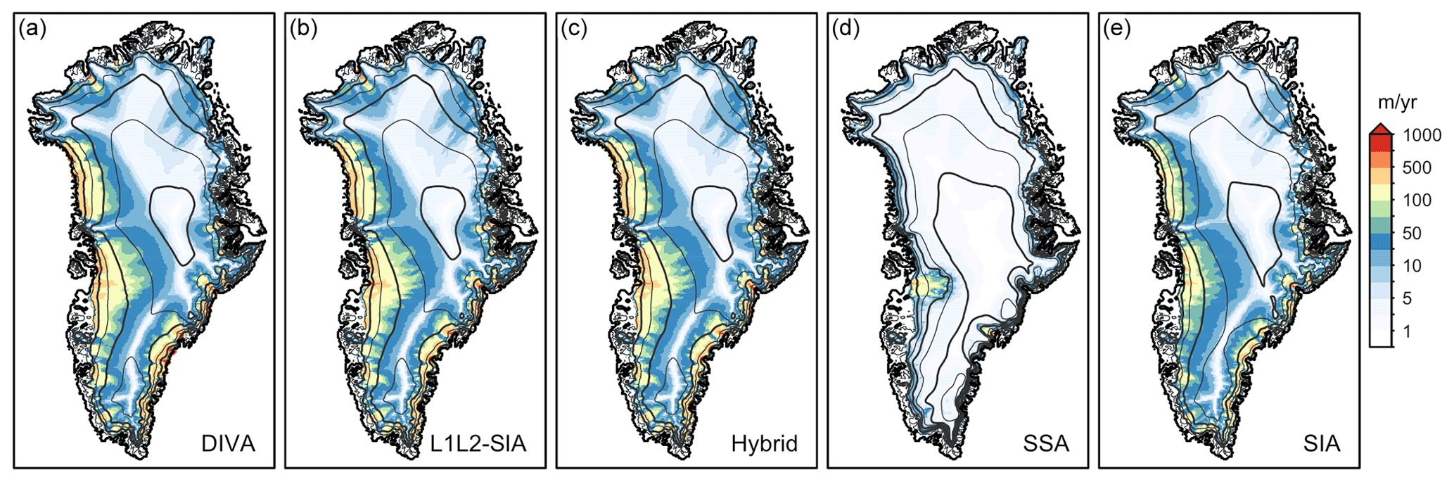
Figure 2Simulated surface velocity (m yr−1) at 8 km resolution at the end of the 3 kyr simulation using the (a) DIVA, (b) L1L2-SIA, (c) Hybrid, (d) SSA and (e) SIA solvers as implemented in the Yelmo ice-sheet model.
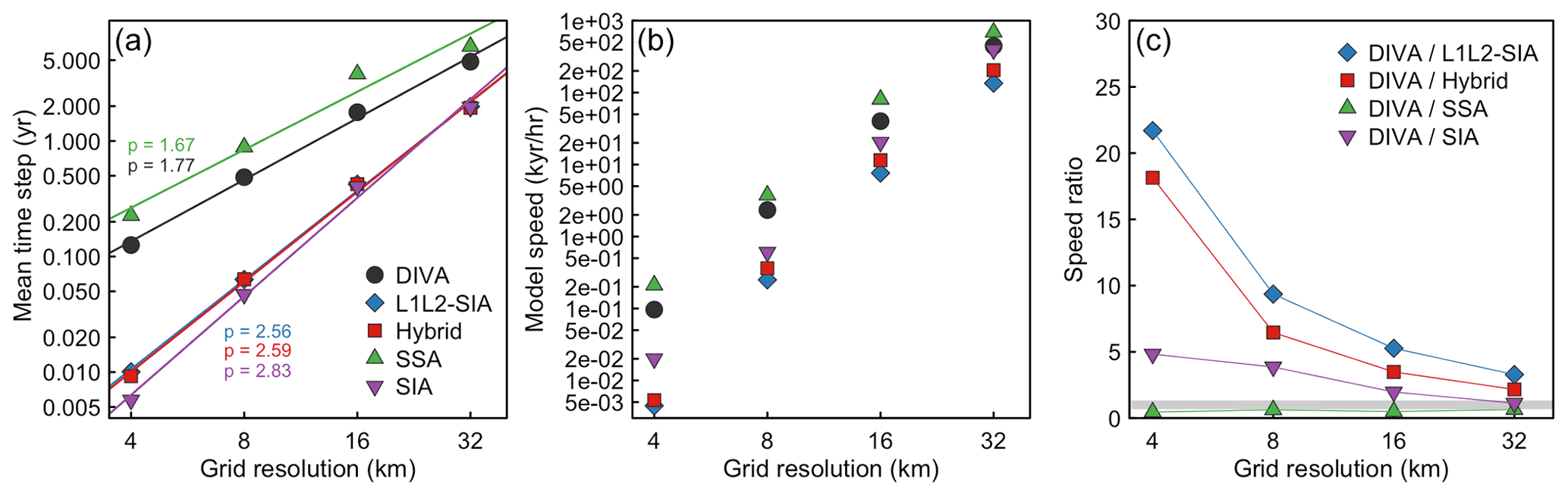
Figure 3(a) Mean model time step, (b) mean model speed (kiloyears model time per hour of computation on one processor) and (c) ratio of the DIVA mean model speed relative to other solvers (a ratio of >1 implies the simulation using the DIVA solver ran faster) versus grid resolution.
An analysis of model stability, illustrated in Fig. 3, shows large, systematic differences among solvers. Two solver families emerge: the SIA and SSA families. For all solvers, the maximum stable time step decreases nonlinearly with increasing grid resolution (Fig. 3a), as shown by the fitted exponent p in the relation Δt∼Δxp. Such a relationship could be expected from the stability analysis in Sect. 3, since the simulations here correspond more closely to the low-resolution regime highlighted in Table 1. The three solvers that rely on the SIA in some form (SIA, Hybrid and L1L2-SIA) have similarly high values of p, ≈2.6–2.8, and thus a large decrease in time step with finer resolution. In contrast, the SSA and DIVA solvers have a much weaker dependence on grid resolution (p≈1.7–1.8), resulting in larger stable time steps. At the coarsest resolution, Δx=32 km, all solvers allow a time step of a similar order of magnitude, between 1–5 yrs, although the SIA family requires time steps more than 2 times smaller than the SSA family. As the resolution increases to Δx=4 km, the SIA family requires time steps of less than Δt=0.01 yr, while the SSA and DIVA solvers remain stable for time steps at least an order of magnitude larger.
We also tested solver performance for a constant time step to ensure that the adaptive time-stepping scheme provides good estimates of the maximum stable time step. We ran simulations for all solvers for the GrIS domain at 16 km resolution with fixed time steps of Δt=0.2, 0.5, 1.0, 2.0 and 5.0 yr. From the simulations with adaptive time stepping, we expect that all five solvers would be stable at Δt=0.5 yr but that the SIA, Hybrid and L1L2-SIA solvers would become unstable for larger time steps. Additionally, we expect that the DIVA solver would become unstable for time steps larger than Δt=1.0 yr and that the SSA solver would be unstable for the largest time step tested here, Δt=5.0 yr. Figure 4 confirms that this is the case. This supports the notion that the adaptive time-stepping scheme successfully diagnoses the maximum stable time step allowed in each simulation.
The difference in maximum stable time step between solvers results in a marked difference in computational speed (Fig. 3b). At lower resolutions, the differences are modest. The SSA and DIVA solvers run about twice as fast as the Hybrid and L1L2-SIA solvers, while the SIA solver is on par with the fastest solvers because it is computationally much less intensive. As the resolution increases, the time step dependency on resolution becomes the limiting factor, and the solvers again separate into the faster SSA family and the slower SIA family.
With the exception of the SIA solver, all solvers are comparable in terms of computational time per time step. Ordered from fastest to slowest per time step, the solver ranking is SIA, SSA, DIVA, Hybrid and L1L2-SIA. The SIA solver does not require any matrix solutions, so it is much less expensive. The SSA solver requires a computationally intensive matrix solution but does not require additional calculations for the 3D horizontal velocity field due to the assumption of no vertical shear. The Hybrid, L1L2-SIA and DIVA solvers use the same 2D matrix-solution method as the SSA solver, and all require some vertical integration as well. The L1L2-SIA solver requires more intermediate calculations than the Hybrid or DIVA solvers, but for a Glen's flow law exponent of n=3, as is the case here, an additional iterative step to determine the effective viscosity for the L1L2-SIA solver can be avoided via an analytical solution. Further analysis (not shown) indicates that all solvers require a similar number of Picard iterations to arrive at the converged matrix solution. This shows that the model time step is the primary determinant of overall model speeds.
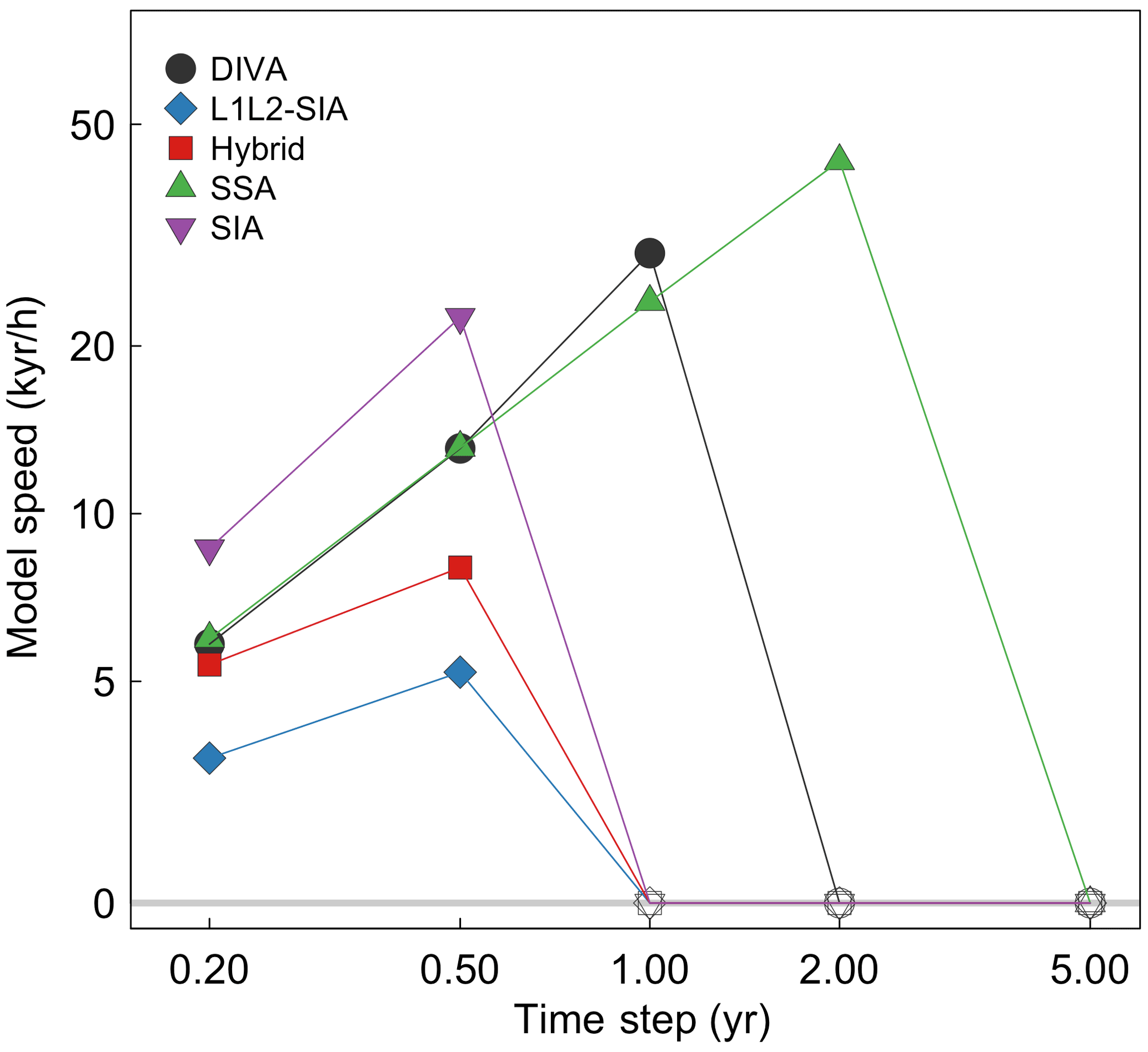
Figure 4Computational speed (kiloyears model time per hour of computation on one processor) versus prescribed time step for simulations of the GrIS at 16 km resolution using the DIVA, L1L2-SIA, Hybrid, SSA and SIA solvers. Empty symbols at a speed of zero indicate simulations that have crashed.
Taking DIVA as a reference, we can benchmark its performance against the other solvers (Fig. 3c). The DIVA solver is comparable in computational performance to the SSA solver at all resolutions, although SSA is systematically faster due to a somewhat larger stable time step and fewer operations per time step. The performance advantage of DIVA over the remaining solvers increases with resolution. DIVA runs about 2–4 times faster than the Hybrid and L1L2-SIA solvers with Δx=32 km and about 20 times faster at Δx=4 km. Interestingly, DIVA also runs faster than the simpler SIA solver at high resolution, reaching speeds up to 5 times faster at Δx=4 km. It may be that the numerical implementation of Yelmo's SIA solver can be improved, but in its current form, the lower computational demand per time step does not offset a time step nearly 2 orders of magnitude smaller than the DIVA time step. Furthermore, the SIA solver does not resolve the same complexity of ice-flow physics. This is also true of the SSA solver, which does perform marginally better than the DIVA solver but cannot represent all large-scale ice-flow regimes.
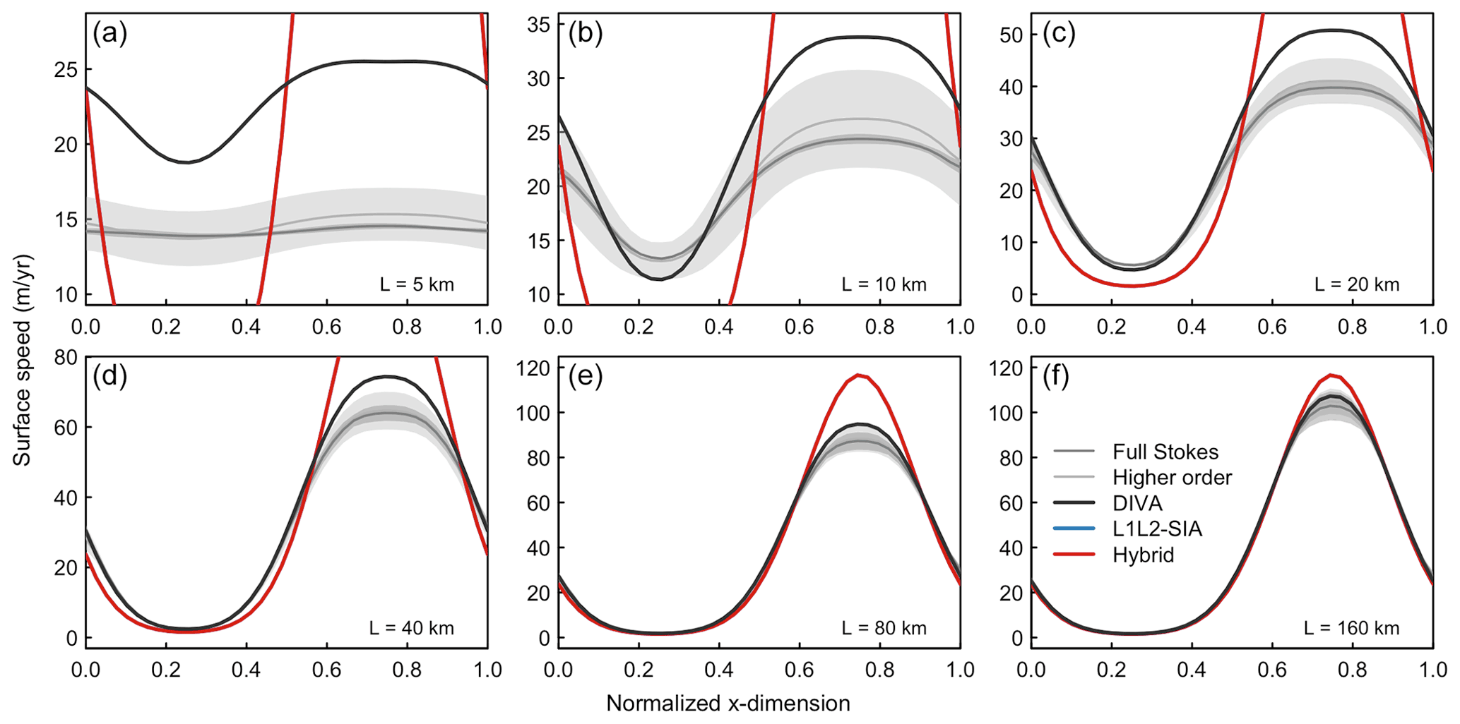
Figure 5Comparison of velocity solutions for the DIVA (black lines), L1L2-SIA (blue lines) and Hybrid (red lines) solvers as implemented in Yelmo to the full Stokes (dark grey lines and bands) and higher-order (light grey lines and bands) solvers used in the ISMIP-HOM benchmark experiment A (ice flow over a bumpy bed with zero sliding; Pattyn et al., 2008) for six length scales (5, 10, 20, 40, 80 and 160 km) in panels (a)–(f), respectively. The L1L2-SIA and Hybrid solutions are identical, both reducing to the local SIA solution in the absence of sliding (thus the lines overlap).
We have shown that different stress-balance approximations can be subject to different stability constraints that are not immediately apparent. The analytical stability analysis in Sect. 3 showed that at low resolution (i.e., Δx>5–10 km), all solvers are subject to a diffusive-like quadratic dependence on grid resolution. Strictly speaking, the stability limit depends on q, which is a function of and H0 as well as Δx. However, resolution is the dominant factor in the tests performed here. At high resolution, two solver families emerge: those whose dynamic time-step limit becomes independent of grid resolution (as shown for the SSA and DIVA solvers) and those whose time-step limit maintains the quadratic dependence. These results were derived for simplified conditions (1D flow with uniform viscosity and constant slope), but the analysis is consistent with Greenland simulations performed without these simplifications.
The L1L2-SIA solver is a notable exception, in that a simplified 1D model with constant viscosity indicates stability akin to the DIVA solver, albeit offset to a lower maximum time-step limit at high resolution. However, when using comprehensive ice-sheet models for either the simplified experiments or the more realistic Greenland experiments, the stability of the L1L2-SIA solver is more consistent with the Hybrid solver. Cornford et al. (2013) noted that using the reconstructed depth-averaged L1L2-SIA velocity in their mass continuity scheme leads to instability as well, and they resort to using only the basal sliding velocity to evolve thickness. Thus it appears to be challenging to implement the L1L2-SIA solver (which is indeed more complex than the other solvers) in a way that retains the more stable time-stepping behavior.
The results of the GrIS experiments confirm the emergence of the two solver families, with the SIA and SSA solvers serving as extreme bounds. The SSA and DIVA solvers show a reduced (less than quadratic) dependence on grid resolution as the grid is refined. The SSA solver maintains a systematically larger time step than DIVA, most likely because vertical shear stress does not contribute to a reduction in stability. In contrast, the SIA, Hybrid and L1L2-SIA solvers show a stronger resolution dependence, with p values in the relation Δt∼Δxp ranging from 2.6–2.8. The SIA solver requires a systematically lower time step than the Hybrid and L1L2-SIA solvers, likely because the driving stress is not dissipated in any way via membrane stresses as in the other two solvers. Analogous simulations for the Antarctic Ice Sheet (not shown), which has large, fast-flowing ice shelves, give similar results as shown here for the GrIS.
The maximum stable time step depends on resolution for all solvers in these realistic tests, in contrast to the 1D and analytical results. At least three factors may contribute to this result. First, the Glen flow law in the realistic tests is nonlinear with n=3. Second, viscosity is no longer constant and therefore makes a highly nonlinear contribution to the solution. Third, ice-front boundary conditions must be considered, which were avoided in the idealized framework. For this reason, the analytical results provide a general guide of the relative stability of the solvers but not a realistic estimate of the stable time step under all conditions.
Continental-scale simulations using Yelmo at higher resolutions than Δx=4 km were not attempted, but the analytical results indicate that a further performance advantage of DIVA could be expected. At such high resolution, factors other than the dynamics, such as basal hydrology and thermodynamics, may play limiting roles in the maximum stable time step. Also, at a high enough resolution, the advective limit will further restrict the time step for the DIVA solver.
All solvers were tested in Yelmo with the same numerical treatment of mass conservation. This served to compare the solvers on an equal basis. However, some of the time-step limitations presented here might be alleviated by the use of mass conservation schemes tailored to the solver in question. For example, applying an implicit scheme to the SIA contribution to velocity can improve stability (Bueler and Brown, 2009). Nonetheless, specific schemes tailored to the choice of dynamics solver, including fully implicit approaches, come with their own tradeoffs and limit the flexibility of the model.
Based on our analysis, the key difference in performance between the two families of solvers emerges in ice-flow regimes that are predominantly driven by vertical shear stress. This is consistent with results of the ISMIP-HOM experiments (Pattyn et al., 2008), which compare the ability of different solvers to reproduce expected features of ice dynamics in an idealized setting. Previous work has shown that, when membrane stresses dominate (experiment C of Pattyn et al., 2008), the DIVA, L1L2-SIA and SSA solvers compare well to the benchmark Stokes solutions for a range of length scales (Pattyn et al., 2008; Goldberg, 2011; Perego et al., 2012). However, when sliding is not permitted and shear stress plays a stronger role (experiment A), the results from all three solvers deviate from those of Stokes solvers as the length scale decreases (Fig. 5). The Hybrid and L1L2-SIA solvers perform quite poorly, as expected, since without sliding, velocities are only represented by the SIA solution. The DIVA solver gives results closer to the Stokes solutions but with decreasing fidelity at smaller length scales (Goldberg, 2011; Lipscomb et al., 2019). From this, we can understand that the solvers that are less stable numerically as resolution increases (those that reduce to SIA) are also those whose representation of ice-flow physics is least robust.
In general, it should be noted that the simple slab test presented here (Sect. 3) serves as an excellent benchmark for testing the maximum stable time step of an ice-sheet model formulation. It is computationally cheap, avoids complications related to lateral boundaries (e.g., calving) and is simple to implement. Most importantly, our results show that the relationship of the maximum stable time step versus resolution determined via this test should be representative of model stability in more realistic experiments.
We have investigated the numerical performance of several commonly used ice-dynamics solvers. We focused on three fast, depth-integrated solvers that permit continental-scale simulations of ice sheets, namely the Hybrid, L1L2-SIA and DIVA solvers. These solvers treat both shear and membrane stresses, so they are appropriate for simulating large-scale ice sheets. We included the SIA and SSA solvers as useful boundary cases that treat only shear or membrane stresses, respectively.
As a first step, we derived expressions for maximum stable time steps for the DIVA, Hybrid and L1L2-SIA solvers in an idealized 1D configuration. This analysis showed that with coarse resolution, the maximum stable time step in all three solvers is proportional to the grid resolution squared (i.e., Δt∼Δx2). For high resolution, the time-step limit in the Hybrid solver maintains this resolution dependence, greatly restricting the time step. In contrast, this term drops out for the DIVA solver, whose maximum stable time step (assuming that stability is not limited by the advective time step) depends only on ice thickness and viscosity. The result is that the DIVA solver may use a larger time step than the Hybrid solver, especially at higher resolutions. The stability analysis shows that only the DIVA solver has similar stability characteristics to the SSA solver. The analysis was inconclusive for the L1L2-SIA solver. A 1D model suggests that its stability should be similar to DIVA, but tests using Yelmo and CISM show that its stability is closer to that of the Hybrid solver.
We next performed quasi-steady-state simulations of the GrIS using the five solvers for grid resolutions ranging from 4–32 km. Two families of solvers emerge, largely consistent with the analytical results. The SSA and DIVA solvers are stable for larger time steps, with a less-than-quadratic dependence on grid resolution. In contrast, the SIA, Hybrid and L1L2-SIA solvers show reduced stability at high resolution, with an overall more-than-quadratic dependence on Δx.
Overall, our analysis shows the DIVA solver to be superior to the Hybrid and L1L2-SIA solvers for reasons of greater numerical stability as resolution increases and preferable to the SIA and SSA solvers because of greater physical fidelity in different parts of the ice sheet. Its representation of the stress balance is consistent with full Stokes solutions over a range of length scales. As continental-scale simulations are performed at higher resolutions, the Hybrid and L1L2-SIA solvers may become bottlenecks for model performance, while the DIVA solver remains computationally efficient.
In this appendix we derive Eq. (43) for u, the solution to Eq. (40). We rescale this linear system as
where the elements of A are
where q is given by
Thus, q is non-negative and is determined by two non-dimensional parameters, and . Here, it is understood that A is circulant. That is, each row is displaced by one element to the right compared to the row above, with ,
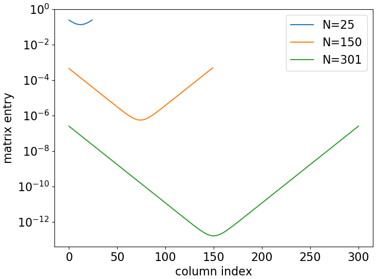
The inverse of A, denoted by A−1, has an approximate analytic expression G (derived in Eq. A2), where the approximation improves exponentially the larger the size of the domain L relative to Lm is, as defined in Eq. (39). The element on row m and column n of G can be written as
where
and
That is, ℒ is the closest distance between m and n accounting for periodicity. Note that q uniquely determines the elements of G. For large q, it can be shown that , and for small q, we have and . For any q>0, we have . Thus, for matrix elements far from the main diagonal (i.e., with sufficiently large ), gm,n becomes negligible compared to a0.
Suppose we define “negligible” as smaller than a0e−p for some p>0. Then the condition for element gm,n to be negligible is or, equivalently, . For small q, where , the condition for negligible matrix elements (recalling that for small x) becomes
Comparing Eqs. (39) and (A3), we find , and therefore Eq. (A8) can be written as MΔx≳pLm. Thus, Lm can be interpreted as a length scale over which the elements of the matrix inverse become small, and the condition Lm≪L ensures that entries far from the diagonal approach zero. Moreover, the expression for G shows that velocity, as obtained by inverting Eq. (A1), is a localized weighted average of driving stress (i.e., the right-hand side of Eq. A1), with Lm as a measure of the averaging kernel.
We refer to the right-hand side of Eq. (A1) as R, with elements Rn. Recall that thickness and velocity points are staggered, with hun located between hn and hn+1, so that and . With δH as in Eq. (36), Rn is given by
where for compactness we have written the large bracketed expression as κ(k,Δx). Pre-multiplying Eq. (A1) by G, the velocity um can be computed as
where the sum is taken over all columns of G with non-negligible entries in row m. The series in Eq. (A10) can be written as a sum of a constant term (i.e., 1) and two series – one corresponding to n>m and the other to n<m. Without loss of generality, we assume and replace by . Further, we assume that N is large enough that the terms in the series are negligible for large . Thus, the two series (n>m and n<m) can be viewed as infinite geometric sums of the form , where z=reikΔx for the first series and for the second series. These infinite series will converge to provided that , which follows from as shown above. This results in the expression given in Sect. 3.1, Eq. (43):
where we have defined a function ϕ that can be simplified and shown to be real:
The matrix A in Eq. (A1) is a circulant matrix with diagonal terms 2+q and first off-diagonal terms −1, and zero elsewhere. Define by am,n the entry at row m and column n of A and by the entry at row m and column n of A−1. Since , the identity matrix, we require that for each row m, the following must hold:
We also require that the inner product of row m of A−1 with any column n of A, m≠n, is zero, i.e.,
We do not derive an analytical expression for a matrix that satisfies Eqs. (B1) and (B2) for all m and n (and we do not know that one exists). Rather, we derive here an analytically defined matrix G which is close to A−1 in the sense that (GA−I) is small. We choose an ansatz G as follows:
where . That is, G is a circulant matrix and ℒ is the distance in columns between m and n but accounting for the circulant property of G. For m≠n, Eq. (B2) yields
yielding the solution
We take only the negative branch of the solution, leading to Eq. (A5). Although this choice is not immediately apparent, it should become clear below. In particular, Eq. (B2) is not satisfied everywhere by G. When (where ⌊⋅⌋ indicates the floor function), the inner product of Gm, the mth row of G, and An, the nth column of A, is
if N is even, and it is
if N is odd. We are interested in the limit of high resolution (i.e., small q) and its influence on stability. As discussed in A1, as q goes to zero, we have , and therefore (using for small x):
from which it can be shown that is asymptotic to e−p, where . (Note that if the positive branch of Eq. B5 were taken, the non-zero off-diagonal entries of GA would instead grow without bound.) Thus, as long as the numerical domain is sufficiently large compared to Lm, the off-diagonal terms of the matrix product GA (and equivalently AG) are bounded by e−p, where the correct choice of a0 (given below) ensures that the diagonal entries are 1. It remains to find a0. Equation (B1) becomes
yielding Eq. (A6). It can be seen numerically (Fig. B1) that the rows of G are a good approximation to those of A−1.
Yelmo is maintained as a Git repository hosted at https://github.com/palma-ice/yelmo (last access: 2 November 2021) under the license GPL-3.0. Model documentation can be found at https://palma-ice.github.io/yelmo-docs/ (last access: 19 December 2021). The exact version of the model used to produce the results used in this paper is archived on Zenodo at https://doi.org/10.5281/zenodo.5791864 (Robinson, 2021) and has been tagged in the repository as solver-stability-v1.0. CISM is an open-source code developed on the Earth System Community Model Portal (ESCOMP) Git repository at https://github.com/ESCOMP/CISM (last access: 17 November 2021). The version used for these runs has been archived on Zenodo at https://doi.org/10.5281/zenodo.5889016 (Lipscomb et al., 2022) and tagged in the repository as cism_slab_tests.
The supplement related to this article is available online at: https://doi.org/10.5194/tc-16-689-2022-supplement.
AR conceived of the study. DG derived and performed the analytical stability analysis with input from WHL. AR performed the experiments with Yelmo, and WHL ran the experiments with CISM. All authors contributed to the analysis of the results and writing of the manuscript.
At least one of the (co-)authors is a member of the editorial board of The Cryosphere. The peer-review process was guided by an independent editor, and the authors also have no other competing interests to declare.
Publisher’s note: Copernicus Publications remains neutral with regard to jurisdictional claims in published maps and institutional affiliations.
Alexander Robinson was supported by the Ramón y Cajal Programme of the Spanish Ministry for Science, Innovation and Universities (grant no. RYC-2016-20587), as well as the Spanish Ministry of Science and Innovation project ICEAGE (grant no. PID2019-110714RA-100). Daniel Goldberg was supported by the Natural Environment Research Council (grant nos. NE/S006796/1 and NE/T001607/1). This material is based upon work supported by the National Center for Atmospheric Research, which is a major facility sponsored by the National Science Foundation under cooperative agreement no. 1852977.
This research has been supported by the Ministerio de Ciencia, Innovación y Universidades (grant no. RYC-2016-20587), the Ministerio de Ciencia e Innovación (grant no. PID2019-110714RA-100), and the Natural Environment Research Council (grant nos. NE/S006796/1 and NE/T001607/1).
This paper was edited by Olivier Gagliardini and reviewed by Mauro Perego and one anonymous referee.
Arthern, R. J. and Williams, C. R.: The sensitivity of West Antarctica to the submarine melting feedback, Geophys. Res. Lett., 44, 2352–2359, https://doi.org/10.1002/2017GL072514, 2017. a
Arthern, R. J., Hindmarsh, R. C. A., and Williams, C. R.: Flow speed within the Antarctic ice sheet and its controls inferred from satellite observations, J. Geophys. Res.-Earth, 120, 1171–1188, https://doi.org/10.1002/2014JF003239, 2015. a, b
Blatter, H.: Velocity and stress fields in grounded glaciers – a simple algorithm for including deviatoric stress gradients, J. Glaciol., 41, 333–344, 1995. a
Bueler, E.: Lectures at Karthaus: Numerical modelling of ice sheets and ice shelves, https://glaciers.gi.alaska.edu/sites/default/files/Notes_icesheetmod_Bueler2014.pdf (last access: 23 February 2022), 2009. a
Bueler, E. and Brown, J.: Shallow shelf approximation as a “sliding law” in a thermodynamically coupled ice sheet model, J. Geophys. Res., 114, F03008, https://doi.org/10.1029/2008JF001179, 2009. a
Cheng, G., Lötstedt, P., and von Sydow, L.: Accurate and stable time stepping in ice sheet modeling, J. Comput. Phys., 329, 29–47, https://doi.org/10.1016/j.jcp.2016.10.060, 2017. a, b, c, d, e, f, g
Cornford, S. L., Martin, D. F., Graves, D. T., Ranken, D. R., Le Brocq, A. M., Gladstone, R. M., Payne, A. J., Ng, E. G., and Lipscomb, W. H.: Adaptive mesh, finite volume modeling of marine ice sheets, J. Comput. Phys., 232, 529–549, 2013. a, b
Dukowicz, J. K.: Reformulating the full-Stokes ice sheet model for a more efficient computational solution, The Cryosphere, 6, 21–34, https://doi.org/10.5194/tc-6-21-2012, 2012. a
Glen, J. W.: The creep of polycrystalline ice, Proc. R. Soc. London A, 228, 519–538, 1955. a
Goelzer, H., Nowicki, S., Edwards, T., Beckley, M., Abe-Ouchi, A., Aschwanden, A., Calov, R., Gagliardini, O., Gillet-Chaulet, F., Golledge, N. R., Gregory, J., Greve, R., Humbert, A., Huybrechts, P., Kennedy, J. H., Larour, E., Lipscomb, W. H., Le clec'h, S., Lee, V., Morlighem, M., Pattyn, F., Payne, A. J., Rodehacke, C., Rückamp, M., Saito, F., Schlegel, N., Seroussi, H., Shepherd, A., Sun, S., van de Wal, R., and Ziemen, F. A.: Design and results of the ice sheet model initialisation experiments initMIP-Greenland: an ISMIP6 intercomparison, The Cryosphere, 12, 1433–1460, https://doi.org/10.5194/tc-12-1433-2018, 2018. a, b, c
Goelzer, H., Nowicki, S., Payne, A., Larour, E., Seroussi, H., Lipscomb, W. H., Gregory, J., Abe-Ouchi, A., Shepherd, A., Simon, E., Agosta, C., Alexander, P., Aschwanden, A., Barthel, A., Calov, R., Chambers, C., Choi, Y., Cuzzone, J., Dumas, C., Edwards, T., Felikson, D., Fettweis, X., Golledge, N. R., Greve, R., Humbert, A., Huybrechts, P., Le clec'h, S., Lee, V., Leguy, G., Little, C., Lowry, D. P., Morlighem, M., Nias, I., Quiquet, A., Rückamp, M., Schlegel, N.-J., Slater, D. A., Smith, R. S., Straneo, F., Tarasov, L., van de Wal, R., and van den Broeke, M.: The future sea-level contribution of the Greenland ice sheet: a multi-model ensemble study of ISMIP6, The Cryosphere, 14, 3071–3096, https://doi.org/10.5194/tc-14-3071-2020, 2020. a
Goldberg, D. N.: A variationally derived, depth-integrated approximation to a higher-order glaciological flow model, J. Glaciol., 57, 157–170, https://doi.org/10.3189/002214311795306763, 2011. a, b, c, d, e, f
Greve, R. and Blatter, H.: Dynamics of Ice Sheets and Glaciers, 1st edn., Springer-Verlag, Berlin, https://doi.org/10.1007/978-3-642-03415-2, 2009. a, b
Hindmarsh, R.: A numerical comparison of approximations to the Stokes equations used in ice sheet and glacier modeling, J. Geophys. Res., 109, F01012, https://doi.org/10.1029/2003JF000065, 2004. a, b
Hindmarsh, R.: The role of membrane-like stresses in determining the stability and sensitivity of the Antarctic ice sheets: back pressure and grounding line motion, Philos. T. R. Soc. A, 364, 1733–1767, https://doi.org/10.1098/rsta.2006.1797, 2006. a, b
Hindmarsh, R. C.: Notes on basic glaciological computational methods and algorithms, in: Continuum mechanics and applications in geophysics and the environment, edited by Straughan, B., Greve, R., Ehrentraut, H., and Wang, Y., 222–249, Springer, Berling, http://nora.nerc.ac.uk/id/eprint/19612/ (last access: 23 February 2022), 2001. a, b
Hutter, K.: Theoretical Glaciology, Mathematical Approaches to Geophysics, 1st edn., edited by: Rikitaki, T. and Hazenwinkel, M., D. Reidel Publishing Company, Dordrecht, Boston, Lancaster, https://doi.org/10.1007/978-94-015-1167-4, 1983. a
Isaacson, E. and Keller, H. B.: Analysis of numerical methods, 1st edn., Courier Corporation, ISBN 9780486680293, 2012. a
Lipscomb, W. H., Price, S. F., Hoffman, M. J., Leguy, G. R., Bennett, A. R., Bradley, S. L., Evans, K. J., Fyke, J. G., Kennedy, J. H., Perego, M., Ranken, D. M., Sacks, W. J., Salinger, A. G., Vargo, L. J., and Worley, P. H.: Description and evaluation of the Community Ice Sheet Model (CISM) v2.1, Geosci. Model Dev., 12, 387–424, https://doi.org/10.5194/gmd-12-387-2019, 2019. a, b, c, d
Lipscomb, W. H., Leguy, G. R., Jourdain, N. C., Asay-Davis, X., Seroussi, H., and Nowicki, S.: ISMIP6-based projections of ocean-forced Antarctic Ice Sheet evolution using the Community Ice Sheet Model, The Cryosphere, 15, 633–661, https://doi.org/10.5194/tc-15-633-2021, 2021. a
Lipscomb, W., Sacks, B., Price, S., Hoffman, M., Martin, D. F., Ranken, D., Hagdorn, M., Salinger, A., Evans, K., Norman, M., Shannon, S., Thayer-Calder, K., Leguy, G., Tezaur, I. K., Kennedy, J. H., Goelzer, H., Kluzek, E., Rutt, I. C., and Iesulauro Barker, E.: ESCOMP/CISM: CISM Slab Tests (cism_slab_tests), Zenodo [code], https://doi.org/10.5281/zenodo.5889016, 2022. a
MacAyeal, D. R.: Large-scale ice flow over a viscous basal sediment – Theory and application to Ice Stream B, Antarctica, J. Geophys. Res., 94, 4071–4087, 1989. a
Morland, L.: Unconfined ice-shelf flow, in: Dynamics of the West Antarctic Ice Sheet, edited by: Van der Veen, C. J. and Oerlemans, J., Glac. Quat. G., 4, 99–116, Springer, https://doi.org/10.1007/978-94-009-3745-1_6, 1987. a
Morland, L. W.: Thermomechanical balances of ice sheet flows, Geophys. Astro. Fluid, 29, 237–266, https://doi.org/10.1080/03091928408248191, 1984. a
Pattyn, F.: A new three-dimensional higher-order thermomechanical ice sheet model: Basic sensitivity, ice stream development, and ice flow across subglacial lakes, J. Geophys. Res., 108, 2382, https://doi.org/10.1029/2002JB002329, 2003. a
Pattyn, F.: Sea-level response to melting of Antarctic ice shelves on multi-centennial timescales with the fast Elementary Thermomechanical Ice Sheet model (f.ETISh v1.0), The Cryosphere, 11, 1851–1878, https://doi.org/10.5194/tc-11-1851-2017, 2017. a
Pattyn, F., Perichon, L., Aschwanden, A., Breuer, B., de Smedt, B., Gagliardini, O., Gudmundsson, G. H., Hindmarsh, R. C. A., Hubbard, A., Johnson, J. V., Kleiner, T., Konovalov, Y., Martin, C., Payne, A. J., Pollard, D., Price, S., Rückamp, M., Saito, F., Souček, O., Sugiyama, S., and Zwinger, T.: Benchmark experiments for higher-order and full-Stokes ice sheet models (ISMIP–HOM), The Cryosphere, 2, 95–108, https://doi.org/10.5194/tc-2-95-2008, 2008. a, b, c, d
Perego, M., Gunzburger, M., and Burkardt, J.: Parallel finite-element implementation for higher-order ice sheet models, J. Glaciol., 58, 76–88, https://doi.org/10.3189/2012JoG11J063, 2012. a, b, c, d, e
Pollard, D. and DeConto, R. M.: Description of a hybrid ice sheet-shelf model, and application to Antarctica, Geosci. Model Dev., 5, 1273–1295, https://doi.org/10.5194/gmd-5-1273-2012, 2012. a
Quiquet, A., Dumas, C., Ritz, C., Peyaud, V., and Roche, D. M.: The GRISLI ice sheet model (version 2.0): calibration and validation for multi-millennial changes of the Antarctic ice sheet, Geosci. Model Dev., 11, 5003–5025, https://doi.org/10.5194/gmd-11-5003-2018, 2018. a, b
Robinson, A.: palma-ice/yelmo: Solver Stability v1.0, Zenodo [code], https://doi.org/10.5281/zenodo.5791864, 2021. a
Robinson, A., Alvarez-Solas, J., Montoya, M., Goelzer, H., Greve, R., and Ritz, C.: Description and validation of the ice-sheet model Yelmo (version 1.0), Geosci. Model Dev., 13, 2805–2823, https://doi.org/10.5194/gmd-13-2805-2020, 2020. a, b, c, d
Schoof, C. and Hindmarsh, R. C. A.: Thin-film flows with wall slip: an asymptotic analysis of higher order glacier flow models, Q. J. Mech. Appl. Math., 63, 73–114, 2010. a, b, c
Seroussi, H., Nowicki, S., Simon, E., Abe-Ouchi, A., Albrecht, T., Brondex, J., Cornford, S., Dumas, C., Gillet-Chaulet, F., Goelzer, H., Golledge, N. R., Gregory, J. M., Greve, R., Hoffman, M. J., Humbert, A., Huybrechts, P., Kleiner, T., Larour, E., Leguy, G., Lipscomb, W. H., Lowry, D., Mengel, M., Morlighem, M., Pattyn, F., Payne, A. J., Pollard, D., Price, S. F., Quiquet, A., Reerink, T. J., Reese, R., Rodehacke, C. B., Schlegel, N.-J., Shepherd, A., Sun, S., Sutter, J., Van Breedam, J., van de Wal, R. S. W., Winkelmann, R., and Zhang, T.: initMIP-Antarctica: an ice sheet model initialization experiment of ISMIP6, The Cryosphere, 13, 1441–1471, https://doi.org/10.5194/tc-13-1441-2019, 2019. a, b
Seroussi, H., Nowicki, S., Payne, A. J., Goelzer, H., Lipscomb, W. H., Abe-Ouchi, A., Agosta, C., Albrecht, T., Asay-Davis, X., Barthel, A., Calov, R., Cullather, R., Dumas, C., Galton-Fenzi, B. K., Gladstone, R., Golledge, N. R., Gregory, J. M., Greve, R., Hattermann, T., Hoffman, M. J., Humbert, A., Huybrechts, P., Jourdain, N. C., Kleiner, T., Larour, E., Leguy, G. R., Lowry, D. P., Little, C. M., Morlighem, M., Pattyn, F., Pelle, T., Price, S. F., Quiquet, A., Reese, R., Schlegel, N.-J., Shepherd, A., Simon, E., Smith, R. S., Straneo, F., Sun, S., Trusel, L. D., Van Breedam, J., van de Wal, R. S. W., Winkelmann, R., Zhao, C., Zhang, T., and Zwinger, T.: ISMIP6 Antarctica: a multi-model ensemble of the Antarctic ice sheet evolution over the 21st century, The Cryosphere, 14, 3033–3070, https://doi.org/10.5194/tc-14-3033-2020, 2020. a
Winkelmann, R., Martin, M. A., Haseloff, M., Albrecht, T., Bueler, E., Khroulev, C., and Levermann, A.: The Potsdam Parallel Ice Sheet Model (PISM-PIK) – Part 1: Model description, The Cryosphere, 5, 715–726, https://doi.org/10.5194/tc-5-715-2011, 2011. a, b, c, d, e
- Abstract
- Introduction
- Ice-dynamics solvers
- Analytical stability limits
- Greenland experiments
- Discussion
- Conclusions
- Appendix A: Velocity derivation in stability analysis
- Appendix B: Approximate matrix inverse G
- Code availability
- Author contributions
- Competing interests
- Disclaimer
- Acknowledgements
- Financial support
- Review statement
- References
- Supplement