the Creative Commons Attribution 4.0 License.
the Creative Commons Attribution 4.0 License.
 | 22 Dec 2022
Anthropogenic and internal drivers of wind changes over the Amundsen Sea, West Antarctica, during the 20th and 21st centuries
Paul R. Holland
Gemma K. O'Connor
Thomas J. Bracegirdle
Pierre Dutrieux
Kaitlin A. Naughten
Eric J. Steig
David P. Schneider
Adrian Jenkins
James A. Smith
Ocean-driven ice loss from the West Antarctic Ice Sheet is a significant contributor to sea-level rise. Recent ocean variability in the Amundsen Sea is controlled by near-surface winds. We combine palaeoclimate reconstructions and climate model simulations to understand past and future influences on Amundsen Sea winds from anthropogenic forcing and internal climate variability. The reconstructions show strong historical wind trends. External forcing from greenhouse gases and stratospheric ozone depletion drove zonally uniform westerly wind trends centred over the deep Southern Ocean. Internally generated trends resemble a South Pacific Rossby wave train and were highly influential over the Amundsen Sea continental shelf. There was strong interannual and interdecadal variability over the Amundsen Sea, with periods of anticyclonic wind anomalies in the 1940s and 1990s, when rapid ice-sheet loss was initiated. Similar anticyclonic anomalies probably occurred prior to the 20th century but without causing the present ice loss. This suggests that ice loss may have been triggered naturally in the 1940s but failed to recover subsequently due to the increasing importance of anthropogenic forcing from greenhouse gases (since the 1960s) and ozone depletion (since the 1980s). Future projections also feature strong wind trends. Emissions mitigation influences wind trends over the deep Southern Ocean but has less influence on winds over the Amundsen Sea shelf, where internal variability creates a large and irreducible uncertainty. This suggests that strong emissions mitigation is needed to minimise ice loss this century but that the uncontrollable future influence of internal climate variability could be equally important.
- Article
(3713 KB) - Full-text XML
- BibTeX
- EndNote


The West Antarctic Ice Sheet (WAIS) is losing ice at an increasing rate (Shepherd et al., 2019) and forms a major source of uncertainty in projections of global sea-level rise (IPCC, 2019). The most rapid ice loss is occurring in the Amundsen Sea sector, where thinning and retreat of the floating ice shelves is causing acceleration of their tributary glaciers (De Rydt et al., 2021). The ice loss is caused by changes in melting of ice shelves by the ocean (Shepherd et al., 2004), but it is not clear why this melting has increased, leading to the current ice-sheet mass imbalance.
Several lines of evidence document the history of ice loss in this region. A synthesis of geological and geophysical datasets implies that the ice-sheet geometry was broadly stable in this region for ∼10 000 years prior to the current retreat (Larter et al., 2014). Sediment records from beneath Pine Island Glacier ice shelf show that its grounding line started to retreat from a prominent seabed ridge in the 1940s, with the ice shelf finally detaching from this ridge in the 1970s (Jenkins et al., 2010; Smith et al., 2017). Ice velocity records from satellite data suggest that Amundsen Sea glacier discharge was accelerating from the earliest observations in the 1970s (Mouginot et al., 2014), while satellite altimetry and interferometry data show glacier thinning and grounding-line retreat occurring since at least the early 1990s (Rignot et al., 2014; Paolo et al., 2015; Konrad et al., 2017). Glacier discharge and thinning have accelerated markedly in recent decades (Mouginot et al., 2014; Paolo et al., 2015; Konrad et al., 2017; Shepherd et al., 2019). Overall, this evidence suggests that ice loss was triggered in the 1940s and evolved slowly but continually thereafter, accelerating from the 1990s onwards.
There are several possible explanations for this history of ice loss. First, there is evidence that the 1940s ice retreat was triggered by a period of strong climate variability associated with the tropical Pacific (Schneider and Steig, 2008; Steig et al., 2012, 2013; Jenkins et al., 2018; Holland et al., 2019). If this is the sole cause of the changes, the climatic anomaly must have been an extremely unusual event because the ice sheet was previously stable for millennia in this region (Larter et al., 2014). Second, it is likely that ongoing ice loss is sustained by a range of ice and ocean feedbacks, including grounding-line retreat towards a deeper bed (Favier et al., 2014), increasing ice damage (Lhermitte et al., 2020), freshwater- and iceberg-induced ocean changes (Bett et al., 2020), and increased access of warm water into sub-ice-shelf cavities (De Rydt et al., 2014). However, the WAIS cannot be experiencing a purely unstable, self-sustaining retreat because the rate of ice discharge remains responsive to ocean variability (Christianson et al., 2016; Jenkins et al., 2018). Finally, an overall warming of the Amundsen Sea over the 20th century may have caused an increase in melting that sustains the current ice loss (Holland et al., 2019; Naughten et al., 2022). Any such centennial change could be caused by a combination of anthropogenic forcing and internal climate variability. All of these different processes may be contributing to the ongoing ice loss, but the relative contributions of a historical trigger, ice–ocean feedbacks, and changes in climatic forcing are not yet known.
The Amundsen Sea is subject to strong wind-driven variability – primarily linked to the tropical Pacific (Lachlan-Cope and Connolley, 2006; Ding et al., 2011; Steig et al., 2012) – that is clearly reflected in ice-shelf melting (Dutrieux et al., 2014; Jenkins et al., 2018) and the ice-sheet response (Christianson et al., 2016; Jenkins et al., 2018). Variable winds modulate the supply of relatively warm Circumpolar Deep Water onto the shelf, driving decadal anomalies in ocean thermocline depth and ice-shelf melting (Thoma et al., 2008; Kimura et al., 2017). This strong decadal variability means that any trends caused by anthropogenic climate forcing may not be detectable in the short ocean and ice-sheet observational records (commencing in the 1990s) or atmospheric reanalysis data (reliable only since 1979).
Climate model simulations suggest that a gradual westerly wind trend occurred over the Amundsen Sea shelf break during the 20th century (Holland et al., 2019). Such westerly wind trends are a very well established response of the Southern Hemisphere climate to anthropogenic forcings (Arblaster and Meehl, 2006; Son et al., 2010; Thompson et al., 2011; Gillett et al., 2013; Bracegirdle et al., 2014, 2020; Goyal et al., 2021; Dalaiden et al., 2022). In ocean simulations, this wind trend drives an increased prevalence of warm decadal ocean anomalies and an increase in ice-shelf melting (Naughten et al., 2022), providing the first evidence that anthropogenic forcings may have contributed to ice loss from the WAIS. However, the importance of these externally forced westerly wind trends has recently been challenged by palaeoclimate reconstructions (Dalaiden et al., 2021; O'Connor et al., 2021a). These reconstructions show that a local deepening of the Amundsen Sea Low dominates the wind trends, leading to easterly trends over the Amundsen Sea shelf. The larger-scale westerly trends are also found in the reconstructions but shifted further north. An analogous deepening of the Amundsen Sea Low in recent decades (since 1979) is thought to be largely driven by natural tropical Pacific variability (Raphael et al., 2016; Meehl et al., 2016; Purich et al., 2016; Schneider and Deser, 2018). Therefore, the reconstructions suggest that 20th-century wind trends over the Amundsen Sea shelf, associated with the local Amundsen Sea Low deepening pattern, were largely internally generated. Thus, the contribution of anthropogenic forcings to centennial wind changes in this region remains unclear.
It is crucial to quantify the contribution of anthropogenically forced climate change to past and future ice loss from the WAIS. If the ice loss is dominated by internal climate variability and ice–ocean feedbacks, it may be unavoidable and/or irreversible on centennial timescales. If the ice loss has a substantial anthropogenic component, it may respond to future reductions in anthropogenic forcing. Quantifying the interplay between these factors is therefore crucial to adaptation and mitigation decisions. It is also important to distinguish the influence of different anthropogenic forcings (e.g. greenhouse gases (GHGs) versus ozone depletion), as their mitigation is different. In this study, we combine palaeoclimate reconstructions and climate model simulations to investigate historical wind trends over the Amundsen Sea and their attribution to different forcings, as well as projected future wind trends and their sources of uncertainty. Since wind-forced ocean variability is known to influence ice loss in the Amundsen Sea, understanding these wind changes is informative about the drivers of change in the WAIS.
2.1 Palaeoclimate reconstructions
Palaeoclimate reconstructions are used to understand historical changes in wind forcing over the Amundsen Sea, which arise through the combined influence of external forcing and internal variability. We use 1∘ resolution annually resolved reconstructions of near-surface zonal winds and sea-level pressure (SLP) spanning 1900 to 2005 from O'Connor et al. (2021a). In addition, for this study, we extend the technique to reconstruct near-surface meridional winds and sea-surface temperatures (SSTs). The reconstructions are created using an offline data assimilation method that combines the temporal variability from a sparse set of climate proxies with the spatial covariance fields obtained from climate model simulations. Annually averaged anomaly states (relative to the 1961–1990 mean) are randomly drawn from climate model output to form a “prior” ensemble, and this prior is used for every year reconstructed (Hakim et al., 2016; Tardif et al., 2019). This ensures that all temporal variance and trends in the final reconstruction are generated from the proxy data rather than the climate model. Proxy data used here include the global PAGES2k proxy database (PAGES2k, 2017), supplemented with additional ice-core accumulation and coral records. This means that the reconstructions are well constrained over West Antarctica and the tropical Pacific, the crucial regions of importance to this study.
O'Connor et al. (2021a) validate this reconstruction against many other data sources, including other palaeoclimate reconstructions, modern atmospheric reanalyses (since 1979), longer-term reanalyses (since 1900), and various Southern Annular Mode (SAM) indices. These datasets draw on a variety of observations, including Antarctic station data, but there are no long-term station data near the Amundsen Sea. Therefore, the most relevant validation compares the reconstruction to modern reanalysis fields, which have been well constrained over the Southern Ocean since 1979 following the onset of satellite infrared sounding (Hines et al., 2000; Marshall, 2003; Marshall et al., 2022). This analysis shows that the reconstructions are most skilful over the South Pacific, owing to the availability of proxy data used in the reconstructions and the dominant climate modes in this region (O'Connor et al., 2021a). The reconstructions are also qualitatively in agreement with those of Dalaiden et al. (2021), who use a different data assimilation method and a proxy database focussed on the southern high latitudes. In Sect. 3.1.3 below, we further validate the reconstructed zonal winds over the Amundsen Sea against ERA5 reanalysis fields and the SLP reconstruction of Fogt et al. (2019).
O'Connor et al. (2021a) pay particular attention to the influence of the climate simulations used as the prior, finding that reconstructed trends are sensitive to the inclusion of anthropogenic forcing in the prior simulations. In this study, we focus on reconstructions using the Community Earth System Model 1 (CESM1) “Pacific Pacemaker” simulations as the prior. This is an ensemble of historical simulations that not only contain all anthropogenic forcings but also have eastern tropical Pacific SSTs constrained to follow observations – the “pacemaker” (Schneider and Deser, 2018). We favour these simulations because they should best represent both externally forced and Pacific modes of variability. O'Connor et al. (2021a) show that this prior creates reconstructions with high skill throughout the South Pacific, and we find that the reconstructions perform well when compared to ERA5 for the time series of interest in this study (see Sect. 3.1.3).
We found that reconstructed near-surface wind trends near the coastal regions of the Amundsen Sea are noisy and deviate significantly from geostrophic winds derived from the reconstructed SLP. The derived geostrophic wind anomalies are also better correlated with ERA5 reanalysis surface wind anomalies. This is unsurprising because the reconstructed SLP patterns show greater skill than near-surface winds (O'Connor et al., 2021a) and should better reflect the large-scale climate modes that are constrained by the remote proxies. Near-surface winds are driven by the same SLP of course but are also influenced by uncertain features of the reconstructed near-surface atmospheric structure. Therefore, throughout this study we use geostrophic wind anomalies from the reconstructed SLP. To make these geostrophic winds most comparable to the climate model winds considered next, a simple near-surface correction was derived by comparing geostrophic and near-surface winds in the CESM1 Large Ensemble, which is described below. The correction consists of rotating the geostrophic winds by 10∘ clockwise and multiplying their amplitude by 0.9. This correction marginally improved the correlation of annual wind anomalies to ERA5 reanalysis winds (see Sect. 3.1.3).
2.2 Climate model simulations
Climate simulations are used to understand the role of anthropogenic forcing in the past and future. By comparing these simulations with the reconstructions, we are also able to estimate the historical role of internal climate variability. We consider near-surface winds, SLP, and SST from a total of 180 simulations within 10 ensembles of simulations using CESM1 under different forcings (Kay et al., 2015; England et al., 2016; Sanderson et al., 2017, 2018; Schneider and Deser, 2018; Deser et al., 2020). The ensembles are fully described in Table 1. Near-surface winds are output at the bottom pressure level of the atmospheric model, whose height varies in time and space but is around 50 m over our domain. The atmospheric model uses a 0.9∘ latitude × 1.2∘ longitude grid, so all winds are binned onto a polar stereographic grid with 200 km resolution to clarify the plotting over the region of interest. SLP and SST fields are considered on the native model atmosphere and ocean grids, respectively.
Table 1Description of the CESM1 model ensembles considered in this study. RCP denotes Representative Concentration Pathway.
Many features of this study are only possible because such a wide range of simulations are available for CESM1. The use of a single model is also necessary to ensure that the responses studied are driven only by the prescribed forcings. However, this also means that our conclusions do not account for model structural uncertainty. Fortunately, the CESM1 features a good representation of winds over the Amundsen Sea (Holland et al., 2019) and contains a faithful representation of the Amundsen Sea Low (England et al., 2016) and its crucial teleconnection to the tropical Pacific (Holland et al., 2019). It also produces a good general representation of a wide range of other variables around Antarctica, including SSTs, SLP, sea ice, ice-sheet surface mass balance (Agosta et al., 2015; Lenaerts et al., 2016), and ocean conditions in the Amundsen Sea (Barthel et al., 2020).
CESM1 does have some biases that are pertinent to the present study. The westerly winds and absorbed shortwave radiation over the Southern Ocean are both too strong (Kay et al., 2016), and, like most climate models, historical CESM1 simulations feature unrealistic Antarctic sea-ice loss and ocean surface warming trends from 1979 (Schneider and Deser, 2018). These sea-surface trend biases do not seem to heavily influence model winds, as the simulations accurately represent pressure trends over the South Pacific (Schneider and Deser, 2018; England et al., 2016) and wind trends over the Amundsen Sea (Holland et al., 2019) over this time period. On centennial timescales, CESM1 wind trends in this region are representative of the wider Coupled Model Intercomparison Project 5 (CMIP5) ensemble (Holland et al., 2019), and we find that the ensemble of CESM1 historical trends comfortably includes the reconstructed historical trends (see Sect. 3.1.2). Despite these encouraging results, it remains possible that the model has an excessive wind response to external forcing, and this should be kept in mind as a source of uncertainty in using the model results to separate the forced and internal components of the circulation history.
This study considers trends during the period 1920–2080, for which most simulations are available (Table 1). This is divided into two equal “historical” (1920–2000) and “future” (2000–2080) periods, which are appropriate to climatic forcing of the WAIS. The year 1920 pre-dates the recent ice-sheet retreat (Smith et al., 2017), a modelled warming of the Amundsen Sea (Naughten et al., 2022), and most anthropogenic climate forcing (Kay et al., 2015). The WAIS was rapidly losing mass well before 2000 (Mouginot et al., 2014; Konrad et al., 2017). Therefore, any changes during 1920–2000 are pertinent to the attribution of the ongoing ice loss. The full consequences of ice-sheet melting will take centuries to emerge, but climatic forcing in the decades prior to 2080 is the subject of immediate adaptation and mitigation decisions.
The central ensemble considered is the CESM1 “Large Ensemble” (LENS) (Kay et al., 2015), a perturbed-initial-condition ensemble from 1920–2100 using known external forcings (GHGs, stratospheric ozone depletion, aerosols, land-use change, solar, volcanic) up to 2005 and the strong radiative forcing RCP8.5 scenario thereafter. All other ensembles use the same model as LENS but with different forcings. By calculating the differences between ensembles with and without particular forcings, we are able to isolate the local climate “responses” to those forcings.
The Pacific Pacemaker (PACE) ensemble is used in the reconstruction prior. PACE uses the same external forcings as LENS but is additionally constrained to follow the observed history of SST anomalies in the central and eastern tropical Pacific Ocean (Schneider and Deser, 2018). In a previous study (Holland et al., 2019), PACE was used to estimate the role of internal variability associated with the tropical Pacific. In the present study this function is performed by the palaeoclimate reconstructions, which allow us to estimate the influence of variability from all sources, Pacific and otherwise. This change in approach has important consequences for the results, as discussed below.
A “pre-industrial control” ensemble (PIctrl) is used to assess the significance of externally forced signals. PIctrl is constructed from a long simulation without external forcings (Kay et al., 2015), by splitting it into 22 non-overlapping 80-year periods and then using the resulting ensemble for both the historical and the future periods.
We consider four ensembles of projections under different future forcing scenarios. LENS experiences an extreme high-forcing scenario, RCP8.5 (van Vuuren et al., 2011). The CESM1 “Medium Ensemble” (MENS) (Sanderson et al., 2018) follows RCP4.5, an intermediate-forcing scenario. The CESM1 “low-warming” ensembles (1.5degC and 2.0degC) are subjected to forcings designed never to exceed global warming of 1.5 and 2 ∘C above pre-industrial levels, targets that are associated with the Paris Agreement (Sanderson et al., 2017). In CESM1, both scenarios require negative net carbon emissions before 2100. Each member of these future ensembles starts in 2005 and is a continuation of a historical member from LENS, so we concatenate the appropriate historical and future simulations in order to study future trends from 2000.
Four further ensembles allow us to determine the individual influences of GHGs, ozone depletion, industrial aerosols, and biomass-burning aerosols (England et al., 2016; Deser et al., 2020). For each of these forcings, we consider an ensemble of “leave-one-out” simulations in which the forcing is held fixed while all other forcings evolve. Subtracting each of these ensembles from LENS isolates the response to each excluded forcing (Deser et al., 2020). For example, we introduce a “no-greenhouse-gas” (XGHG) ensemble, which uses the same forcings as LENS apart from GHG concentrations, which are fixed at the 1920 level. We then derive the “GHG response” by subtracting XGHG from LENS, yielding the influence of GHGs that are increasing in LENS but fixed in XGHG. This procedure is repeated for each of the forcings. An advantage of this leave-one-out methodology is that the derived difference includes nonlinear interactions between the excluded forcing and all other forcings.
We consider a set of such climate responses, defined as the difference in ensemble-mean winds between two ensembles that have a difference in forcing. This has the advantage that the significance of a response trend can be assessed by comparing the distributions of wind trends in the two ensembles. Specifically, we conduct a two-sample t test with unequal sample size and variance to test the null hypothesis that the ensembles have the same mean trend, and we treat the response as significant if that hypothesis is rejected at the 95 % confidence level (two-sided). For example, the GHG wind trend response is significant if the distribution of LENS ensemble trends differs from the distribution of XGHG ensemble trends. We note that the number of simulations in each ensemble varies (Table 1) and that this affects the significance of the derived responses.
3.1 Historical changes
3.1.1 Global patterns of change
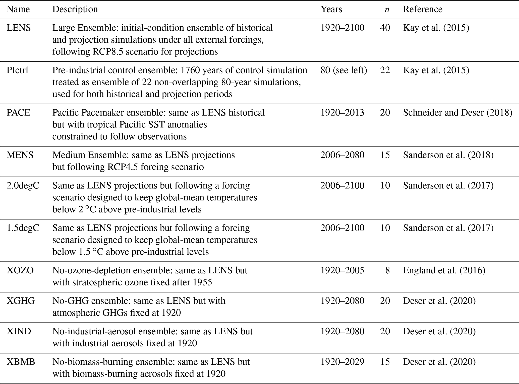
Figure 1a shows a global map of the reconstructed historical trends in SST and SLP. We re-iterate that this reconstruction is most skilful over the South Pacific, the focus of this study, and may be less trustworthy in other regions (O'Connor et al., 2021a). The reconstruction shows a widespread SST warming, particularly strong in the eastern and central tropical Pacific and a strengthening and southward shift of the Southern Hemisphere westerly winds (O'Connor et al., 2021a). Crucially, there is a substantial regional deepening of SLP over the Amundsen Sea.
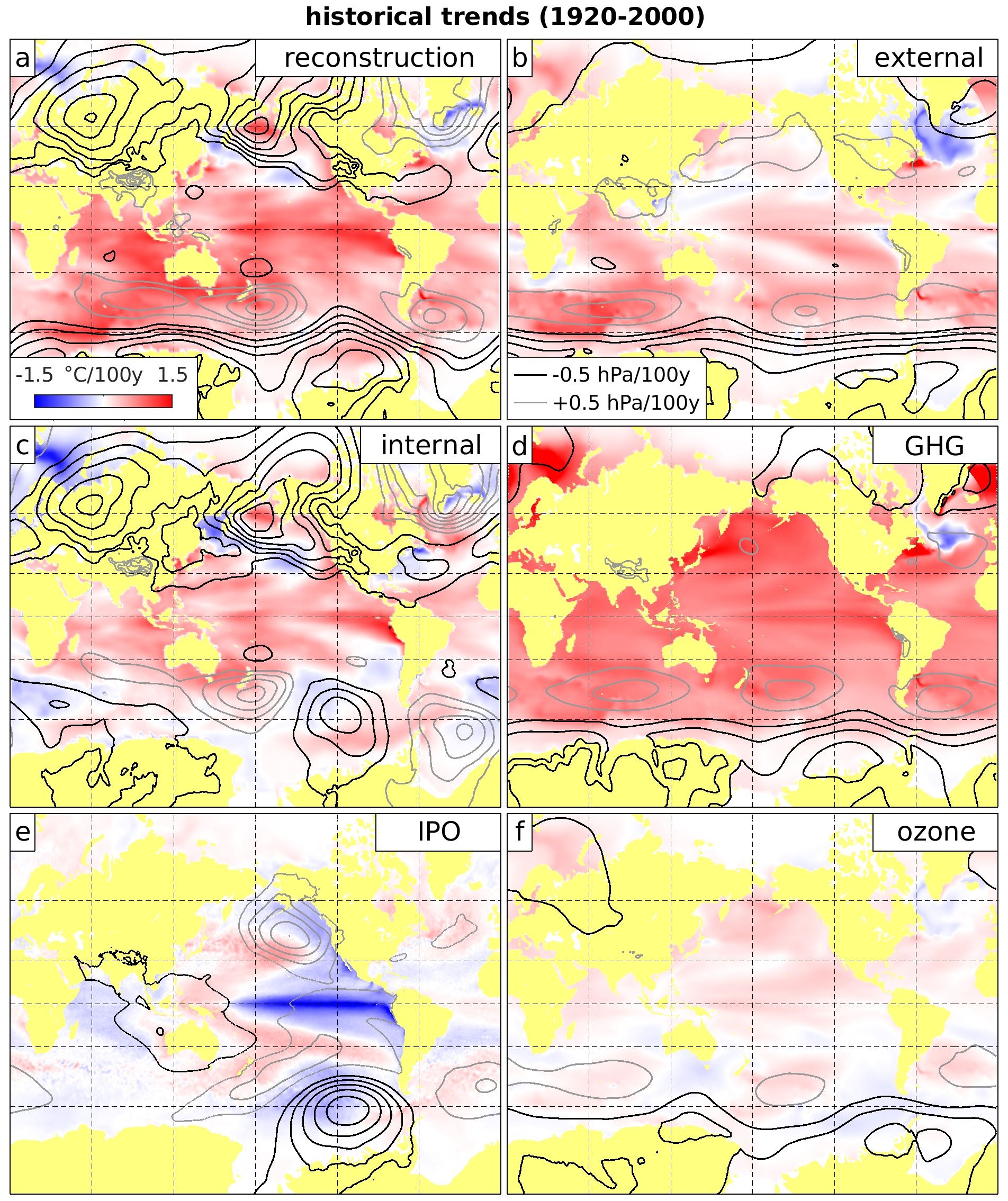
Figure 1Global trends in sea-surface temperature (colour) and sea-level pressure (contours) over the historical period. For SLP, positive and negative contours are plotted in grey and black, respectively, and the zero contour is omitted. (a) Trends in the palaeoclimate reconstruction. (b) Trends caused by external forcing. (c) Trends associated with internal variability (panel a minus panel b). (d, f) Trends caused by greenhouse-gas forcing and ozone depletion, respectively. (e) Trends associated with a hypothetical trend of −1 ∘C per century in the Interdecadal Pacific Oscillation index.
We interpret these features by separating their climatic drivers using the climate model simulations. Figure 1b shows the total externally forced changes (from GHGs, ozone depletion, aerosols, land-use change, solar, and volcanic sources) during this period, which is estimated as the ensemble mean of the LENS trends. The LENS members contain 40 different random realisations of internal climate variability, but they all have the same external forcing. Thus, if we average over all members, the internal variability cancels out, and the externally forced trends appear. This estimate agrees with many previous studies that show historical external forcing drove broad background warming over the South Pacific (e.g. Deser et al., 2020; IPCC, 2019) and a zonally uniform southward shift and acceleration of the westerlies (e.g. Arblaster and Meehl, 2006; Goyal et al., 2021).
We isolate the contribution of individual external forcings using the set of leave-one-out ensembles, as described above. The GHG response in Fig. 1d is derived by subtracting the XGHG ensemble-mean trends from the LENS ensemble-mean trends, since the only difference between these ensembles is the increasing GHGs in LENS. The historical increase in atmospheric GHG concentrations causes a strong SST warming (Fig. 1d), which exceeds the total externally forced warming (Fig. 1b) because aerosol forcing drove cooling during this period (not shown), particularly in the Northern Hemisphere (Deser et al., 2020). GHG forcing drove over half of the historical changes in the westerly winds (Arblaster and Meehl, 2006; Gillett et al., 2013; Dalaiden et al., 2022). Similarly deriving an “ozone response” in Fig. 1f by subtracting XOZO from LENS, we see that ozone depletion drove no strong SST trends but made a substantial contribution to the wind trends (Thompson et al., 2011; Son et al., 2010). The ozone wind response is slightly weaker than the GHG wind response because ozone depletion is only influential in summer months and our chosen historical trend period includes many decades before the onset of rapid ozone depletion. Aerosols drove no substantial Southern Hemisphere wind trends over this period and are not considered further.
By subtracting the externally forced changes in Fig. 1b from the total reconstructed trends in Fig. 1a, we may estimate the part of the trends caused by internally generated variability (Fig. 1c). This approach requires that the reconstruction is consistent with the LENS simulations. We are confident this is the case because the reconstructed trends sit comfortably within the LENS ensemble (Sect. 3.1.2), and the reconstruction uses CESM1 simulations as its prior ensemble (Sect. 2.1). Figure 1c reveals a coherent pattern of alternating SLP anomalies over the South Pacific that feature a prominent trend towards low pressure over the Amundsen Sea. These SLP trends are also supported by SST trends, with warm anomalies wherever the associated wind trend is southward and cold anomalies wherever it is northward (Ciasto and Thompson, 2008). This demonstrates that the reconstructed historical deepening of the Amundsen Sea Low (Dalaiden et al., 2021; O'Connor et al., 2021a) is primarily internally generated. External forcing drives a strong annular SLP trend but makes a much smaller contribution to the local trend anomaly pattern, i.e. the deviation from zonal-mean trends (Fig. 1b). The pattern of alternating SLP anomalies in Fig. 1c is suggestive of a Rossby wave train, a well-established mechanism for the poleward propagation of atmospheric anomalies over the South Pacific (Karoly, 1989; Lachlan-Cope and Connolley, 2006; Ding et al., 2011; Steig et al., 2012; Holland et al., 2019). However, the anomaly pattern also contains features that are unusual.
It is well known that Pacific modes of variability – e.g. the El Niño–Southern Oscillation (ENSO) and Interdecadal Pacific Oscillation (IPO) – induce a global-scale atmospheric response that is highly influential over the Amundsen Sea (Karoly, 1989; Lachlan-Cope and Connolley, 2006; Ding et al., 2011; Steig et al., 2012; Dutrieux et al., 2014; Jenkins et al., 2018; Holland et al., 2019). Figure 1e illustrates the spatial structure of the IPO response. This panel is constructed from the regression of monthly ERA5 reanalysis SLP and SST fields (Hersbach, 2020) onto the IPO tripole index (Henley et al., 2015) during the period 1979–2020. To compare this panel with the others, it is plotted as the response of SLP and SST to a hypothetical trend of −1 ∘C per century in the IPO index. (For example, the hypothetical SLP trend (hPa per century) is calculated by multiplying the SLP regression onto the IPO index () by the hypothetical trend in the IPO index (−1 ∘C per century).) The illustrative value of −1 ∘C per century was arbitrarily chosen to produce a deepening pressure over the Amundsen Sea (Fig. 1e) that is comparable to the internally generated trend in the reconstruction (Fig. 1c).
Comparing Fig. 1c and e suggests that the reconstructed internally generated trends cannot be simply related to the classical IPO and ENSO modes of Pacific variability. Trends associated with these modes typically feature a zonal dipole of SST and SLP anomalies over the tropical Pacific, and a Rossby wave train radiating southwards from the western tropical Pacific (Fig. 1e). Instead, the internally generated trends appear to originate in the subtropical South Pacific at approximately 30∘ S (Fig. 1c). Crucially, the deepening pressure trend over the Amundsen Sea in the reconstruction occurs alongside a warming of the eastern tropical Pacific (Fig. 1c), not the cooling expected from IPO or ENSO variability (Fig. 1e). We conclude that the internally generated trends are not associated with these classical modes but do follow a similar (Rossby wave) propagation. Similar results are obtained with an alternative palaeoclimate reconstruction (Quentin Dalaiden, personal communication, 2022). It is not necessarily surprising that this centennial variability has a different pattern to interannual (ENSO) and interdecadal (IPO) variability. Little is known about variability on these centennial timescales. It is important to note that this discussion refers only to 80-year trends, which arise through the residual of many shorter IPO and/or ENSO anomalies of opposing sign. This aspect is revisited in Sect. 3.1.3 below.
3.1.2 Winds over the Amundsen Sea
Figure 2 has the same six panels as Fig. 1 but with the analysis repeated for near-surface wind trends rather than SLP and SST and focussing on the Pacific sector of the Southern Ocean. The magenta boxes show three areas of the Amundsen Sea that illustrate wind changes of potential relevance to the WAIS – shelf sea, shelf break, and deep ocean. The wind trends reflect the SLP trends in Fig. 1. Figure 2a shows the reconstructed historical wind trends, with vectors coloured black if either the zonal or the meridional wind trend is significant relative to the interannual variability in the reconstruction. The reconstruction features significant westerly wind trends over almost the entire Southern Ocean, apart from the Amundsen Sea shelf. A cyclonic pattern of wind trends is centred on the Amundsen Sea shelf break, arising from the deepening pressure trend in Fig. 1a. This means that the westerly trends to the north transition to easterly trends near the Amundsen Sea coast.
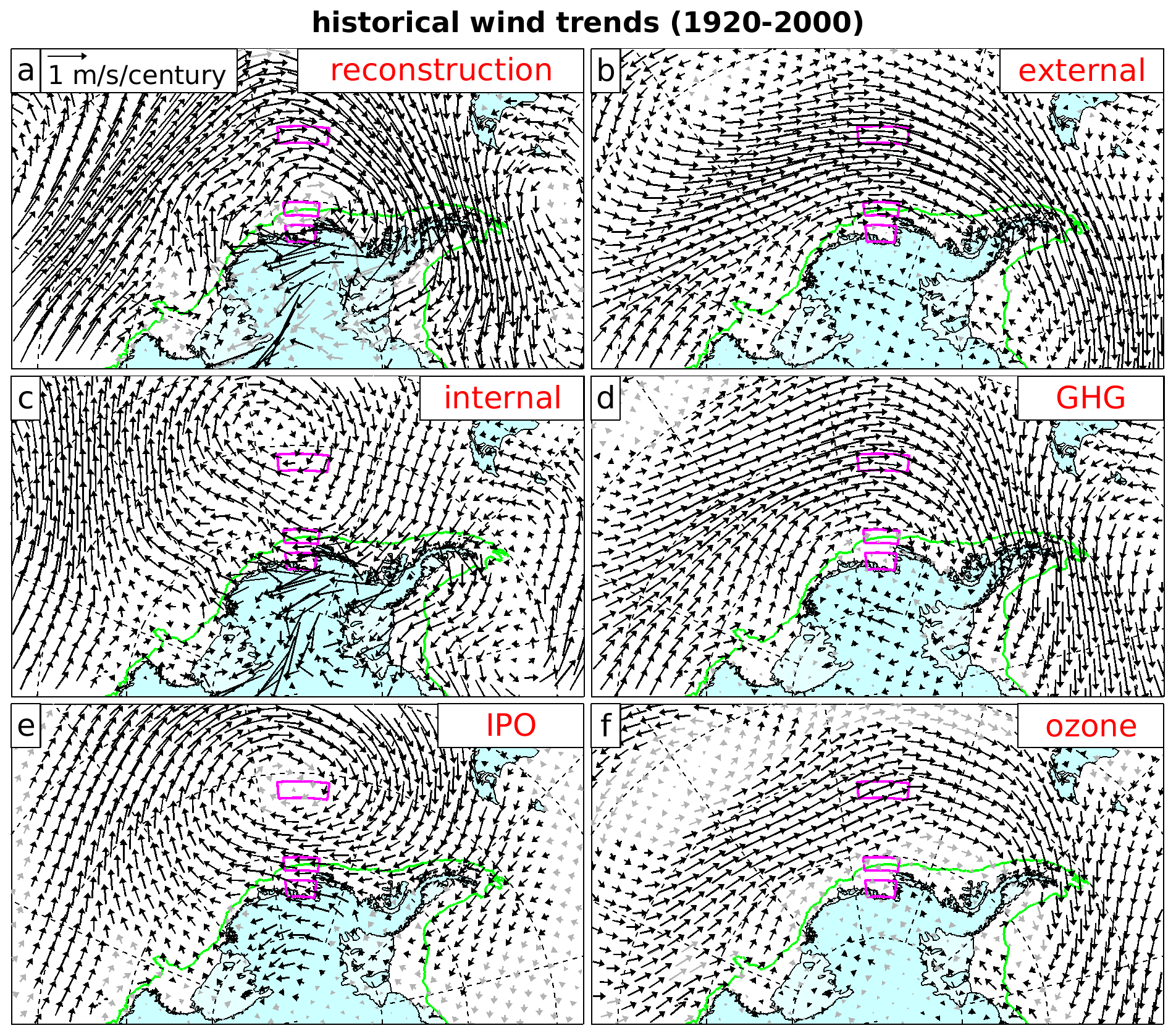
Figure 2Historical trends in near-surface winds over West Antarctica and the South Pacific. The panels are the same as Fig. 1. Black vectors have a zonal or meridional wind trend significant at the 95 % confidence level. The significance test is different for the different panels (see main text). The green contour is the 1000 m isobath at the continental shelf break. Magenta boxes show three selected regions of interest, including (south to north) the Amundsen Sea shelf, shelf break, and deep ocean. These are the locations of time series in Figs. 4–6.
Figure 2b, d, and f show the externally forced wind trends derived from the climate model simulations. These figures are derived in the same way as their counterparts in Fig. 1. Wind trend vectors are coloured black if either the zonal or the meridional wind trend is significant according to a two-sample t test that compares the distribution of trends within two ensembles. For example, in Fig. 2b the externally forced wind trends are estimated as the LENS ensemble-mean trends. At each location, these are considered significant if the distribution of trends in the LENS ensemble has a significantly different mean from the distribution of trends in the PIctrl ensemble under the t test. Figure 2d shows the GHG-induced trends derived by subtracting XGHG ensemble-mean trends from LENS ensemble-mean trends, with vectors shown as significant if the distributions of trends in LENS and XGHG have a different mean under the t test. Figure 2f is the same for ozone.
Figure 2b, d, and f show that the historical westerly wind trends are clearly associated with radiative forcing from GHGs and ozone depletion (Arblaster and Meehl, 2006; Son et al., 2010; Thompson et al., 2011; Gillett et al., 2013; Dalaiden et al., 2022). In a feature that may be important to climatic forcing of the WAIS, these anthropogenic changes are strongest over the deep ocean but not significant over the Amundsen Sea shelf. The shelf break sits in a transition zone, where externally forced trends are significant overall (Fig. 2b), but neither GHG nor ozone responses are significant individually (Fig. 2d and f). This spatial pattern of response to external forcings is also found in the wider ensemble of climate models (Bracegirdle et al., 2014). The broader westerly trends are driven by meridional gradients in atmospheric warming (Harvey et al., 2014; Shaw, 2019), but local controls on wind trends over the Amundsen Sea are complex and require further study.
Over the time period considered, internal variability induces wind trends of magnitude comparable to the externally forced trends (Fig. 2c). As expected from the deepening SLP trends described above, these internally generated wind trends have a cyclonic orientation, centred over the deep ocean north of the Amundsen Sea. As a result, internal variability is associated with an easterly trend over the Amundsen Sea, in direct opposition to the externally forced westerly trend. The internally generated trends are strongest on the shelf and weaken to the north, in contrast to the externally forced trends. Considering this region alone, the internally generated trends closely resemble those expected from the hypothetical negative trend in the IPO index (Fig. 2e).
As mentioned above, it is important to understand the level of consistency between the palaeoclimate reconstruction and climate model simulations, since the role of internal variability is derived by taking their difference. Since the reconstructions use CESM1 simulations as their prior ensemble, in principle there is no structural difference between the two. This can be illustrated by comparing the reconstruction to individual simulations from the LENS ensemble. The LENS ensemble members all have the same externally forced trends but have 40 different realisations of the trends generated by internal variability. Figure 3 shows the reconstruction (top row) alongside two ensemble members chosen manually to illustrate the range of internal variability (other rows). For each of these sources, both the total historical trends (left panels) and the internally generated part only (right panels) are shown. The internally generated trends are calculated, as before, by subtracting the externally forced trends (the LENS ensemble mean) from the total trends. The LENS ensemble members produce a wide variety of internally generated trends. By chance, LENS member 9 has a realisation of internal variability that produces cyclonic trends, with a similar influence over the Amundsen Sea to the reconstruction. This is not unusual within the ensemble and illustrates the consistency between the reconstruction and LENS. By contrast, LENS member 18 exhibits anticyclonic internally generated trends. This highlights the importance of the reconstruction to this study. Without the reconstruction, we would have to treat all LENS members as being equally plausible estimates of the real historical trends and would not be able to constrain the important role of internal climate variability.
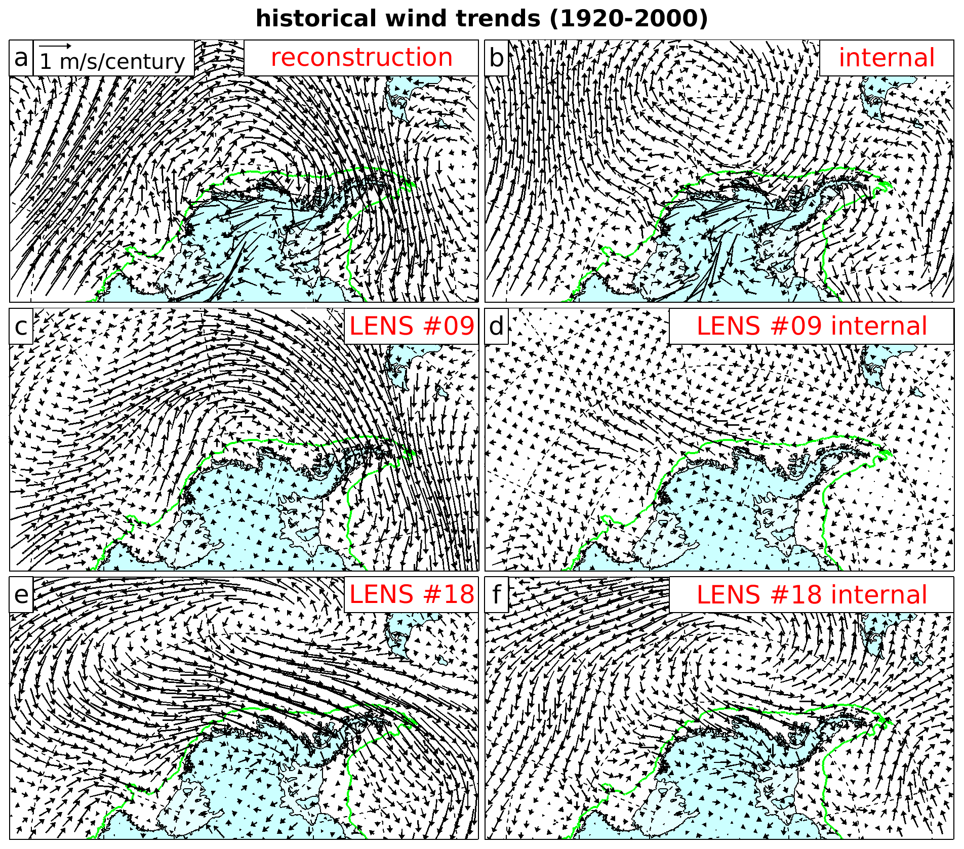
Figure 3Comparison between palaeoclimate reconstruction and selected LENS ensemble members. (a) Reconstructed historical wind trends. (c, e) Wind trends in selected illustrative ensemble members. (b, d, f) Deviation of each of these fields from the externally forced trends in the LENS ensemble mean, illustrating the role of internal climate variability in each field.
3.1.3 Temporal evolution of the anomalies
So far, we have only considered 80-year historical wind trends, but there is substantial variability in the winds on shorter timescales, and this is known to influence WAIS ice loss (Christianson et al., 2016; Jenkins et al., 2018). Figure 4 shows time series of zonal wind anomalies within the three magenta regions shown in Fig. 2 during 1900–2020, the full time period of the palaeoclimate reconstruction and ERA5 reanalysis. The regions extend zonally from 102–115∘ W and meridionally from 73–75∘ S (shelf), 70.2–71.8∘ S (shelf break), and 61–63∘ S (deep ocean).

Figure 4Historical evolution of zonal wind anomalies during 1900–2020. Time series are calculated in the three regions highlighted in Fig. 1 from the palaeoclimate reconstruction and ERA5 reanalysis. Thin lines show annual anomalies, while thick lines show the 13-year running mean, selected because it is characteristic of the Interdecadal Pacific Oscillation. The 1920–2000 trend lines are solid if the trend is significant at the 95 % confidence level and dashed otherwise. Anomalies are plotted relative to mean values over 1979–2005, the period of overlap between the reconstruction and ERA5. Statistics are given for the correlation between datasets during this overlap.
The statistics shown in each panel quantify the interannual correlation in zonal wind anomalies between the reconstruction and ERA5 during their period of overlap, 1979–2005, showing that the reconstruction skill is higher over the deep ocean and decreases towards the south (O'Connor et al., 2021a). This validation may be extended further back in time using zonal winds derived from the interpolated station-based SLP reconstructions of Fogt et al. (2019). These seasonal reconstructions are averaged to produce annual-mean fields, and geostrophic winds are converted to near-surface winds using the simple correction described in Sect. 2.1. These derived winds are correlated to ERA5 only over the deep-ocean region (r=0.44, p=0.01, 1979–2013). In this region, zonal wind anomalies derived from O'Connor et al. (2021a) and Fogt et al. (2019) are correlated to each other with r=0.49, p<0.01, during 1957–2005. This agreement is encouraging given the complete independence of these datasets and the remoteness of their observational constraints from the Amundsen Sea.
Consistent with the cyclonic trends in Fig. 2a, over the 1920–2000 period the reconstruction features westerly trends in the deep ocean, no trend at the shelf break, and easterly trends over the shelf (Fig. 4). However, there is substantial variability in all three regions on both interannual and interdecadal timescales. Several large multi-annual anomalies are visible in the record, which overall appears to be dominated by interdecadal variability. Shelf-break winds contain variability that reverses on a timescale of approximately 50 years (Fig. 4b). We are not aware of any previous studies documenting this slow wind variability in this region, which may be crucial to the WAIS.
In principle, this wind variability arises through a combination of external forcing and internal climate variability. In common with the previous sections, the individual contributions can be separated by combining reconstructions and simulations. Figure 5 shows time series of the separate contributions to the zonal wind anomalies, for the three selected regions, over the historical and future time periods. The two columns both show the same annual time series in thin lines but then emphasise either interdecadal evolution (left) or centennial trends (right) in thick lines. The total externally forced zonal wind anomalies for each location are the LENS ensemble mean. Historical GHG-forced and ozone-forced anomalies are the LENS ensemble mean minus the XGHG and XOZO ensemble means, respectively. The internally generated anomalies are the reconstructed anomalies minus the externally forced anomalies (the LENS ensemble mean).
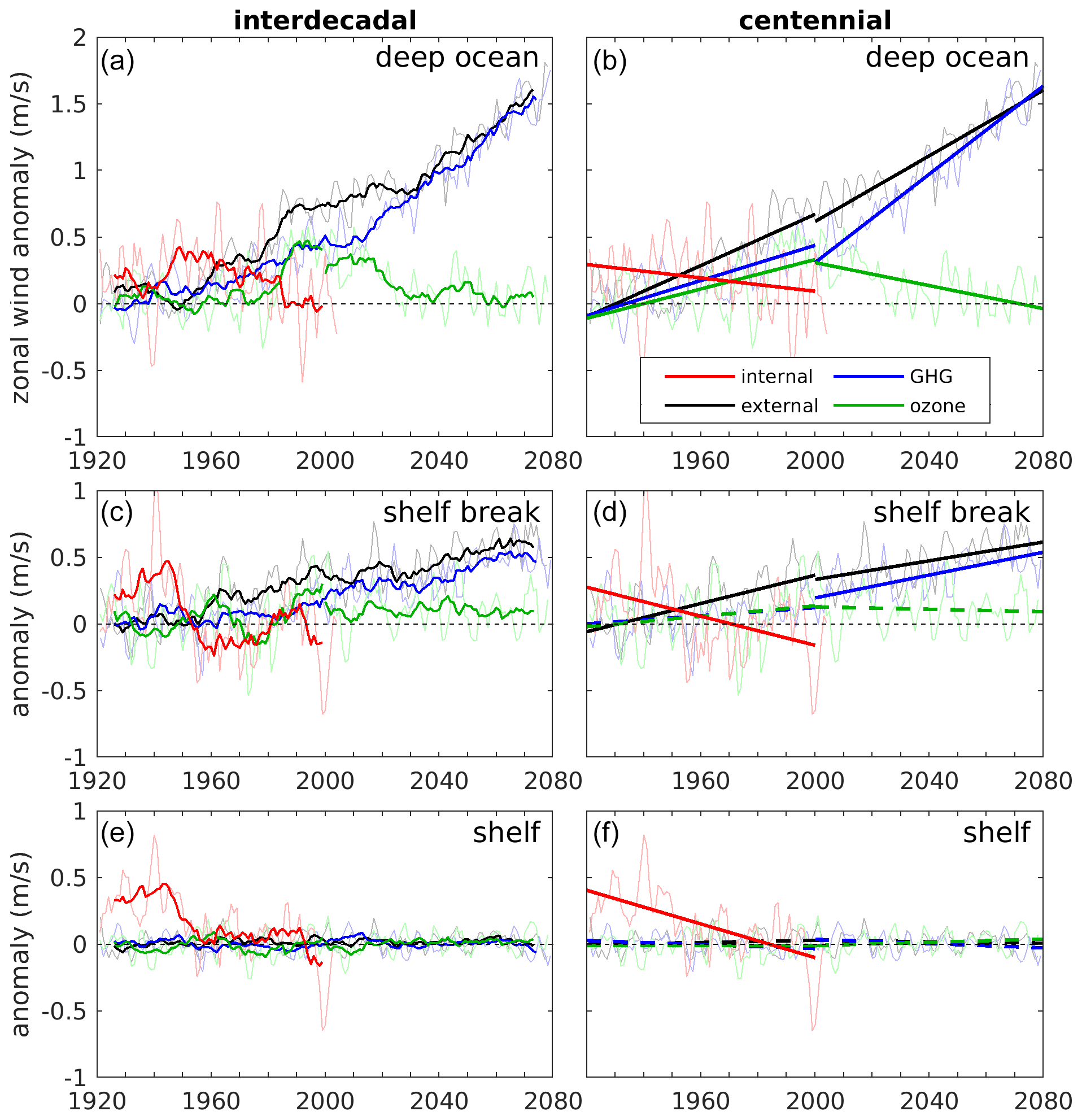
Figure 5Historical and future influences on zonal wind anomalies. Panels show the internally generated, total externally forced, and GHG- and ozone-forced contributions to wind changes in the three regions shown in Fig. 2. Future changes are shown under the strong-forcing RCP8.5 scenario. All panels show annual-mean time series (thin lines). Panels (a), (c), and (e) also show the same time series after a 13-year running mean (thick lines) to highlight the interdecadal evolution of the responses. Panels (b), (d), and (f) also show historical and future trends, plotted solid if the trend is significant at the 95 % confidence level (see text) and dashed otherwise. Ozone is plotted as the ozone response before 2000 and the non-GHG response afterwards. Internally generated anomalies are plotted relative to 1979–2005, as in Fig. 4.
Significant externally generated westerly wind changes occur over the deep ocean and shelf break during the historical period (Fig. 5a–d, black lines). Over the deep ocean, GHG-forced changes are established from approximately 1960 onwards, while ozone-induced changes increase rapidly after approximately 1980 (Fig. 5a, blue and green lines). This leads to significant historical GHG- and ozone-forced trends (Fig. 5b). As noted above, the shelf-break region sits in a transition zone where the forced responses are much weaker (Fig. 5c). While the overall externally forced trend is significant, neither the GHG-forced nor the ozone-forced trends are significant individually (Fig. 5d). There are no significant externally forced changes over the shelf region (Fig. 5e and f). All of these results are consistent with the spatial patterns in Fig. 2, since the derivation of the trends and significance test are identical.
The internally generated variability is substantial in all regions and shows many important features (Fig. 5, red lines). Annual anomalies (thin red lines) are large in amplitude relative to the externally forced changes. A particularly large westerly wind anomaly occurred over the shelf and shelf break in 1940 (Fig. 5c and e), which is clearly part of an anticyclonic feature as it is accompanied by an easterly anomaly over the deep ocean to the north (Fig. 5a). The exceptional strength of this climatic anomaly is well known from ice cores (Schneider and Steig, 2008; Steig et al., 2013), which are constraining the reconstruction here. Interdecadal anomalies (thick red lines, left column) also show substantial variability. This variability broadly shows a 50-year reversal, with opposing easterly and westerly anomalies between the deep ocean and shelf break. Internally generated easterly trends (right column) are also large and play an important role in counteracting the externally forced westerly trends. At the shelf break the externally forced trend is cancelled out completely by the internally generated trend, while in the deep ocean approximately half of the externally forced trend is cancelled out. On the shelf, all variability and trends are internally generated.
Given the known importance of Pacific variability to this region, Fig. 6 examines the extent to which this internal variability is related to the IPO tripole index. This index is based on the temperature difference between tropical and subtropical Pacific SSTs (Henley et al., 2015) from the HadISST1.1 dataset (Rayner et al., 2003). The IPO emerges only on long timescales (Newman et al., 2016), so this index is usually calculated from monthly SSTs and then subjected to a 13-year filter to yield the IPO. In Fig. 6, we plot the standardised annual-mean and 13-year-mean time series of both the IPO index and the reconstructed internal variability in zonal winds. The statistics of the annual-mean and 13-year-mean correlations are shown in each panel. For the deep-ocean region the correlations are negative, so the IPO index is reversed in Fig. 6a for illustrative purposes.
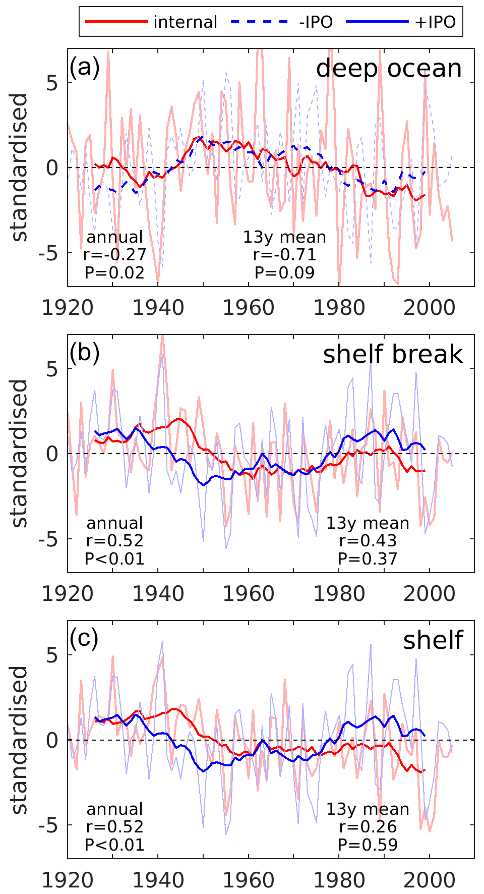
Figure 6Evolution of internally generated zonal wind anomalies and their relationship to the Interdecadal Pacific Oscillation. Panels show the internally generated anomalies and IPO index in the three regions shown in Fig. 2. Thin lines show annual anomalies, while thick lines show a 13-year running mean. All time series are standardised by the 13-year-running-mean data. The IPO index is inverted in panel (a) for illustrative purposes because its correlation to wind anomalies is negative in the deep-ocean region. Statistics show the correlation between the two time series on annual and 13-year timescales.
Annual anomalies in reconstructed internal variability are significantly correlated to the annual-mean values of the IPO index in all regions (Fig. 6). While the correlation coefficients are modest, this significance is remarkable considering the independent origin of these datasets. The IPO index is obtained from optimal interpolation of historical ocean temperature measurements (Rayner et al., 2003), while the internal variability in winds is derived by combining climate model simulations and a reconstruction that uses proxy records from ice cores, tree rings, and coral records. The most extreme annual events in the record, around 1940 and 2000, seem very well explained by the tropical Pacific. The reversing sign of the correlations between shelf and deep ocean illustrates the fact that a positive ENSO or IPO anomaly is associated with anticyclonic wind anomalies associated with a local high-pressure anomaly (Holland et al., 2019).
Unfortunately, there are insufficient data to assess the linkage on longer timescales. The 13-year-mean internally generated wind anomalies are not significantly correlated to the IPO (Fig. 6), which is unsurprising given that there are only ∼70 years of data, and there appears to be a ∼50-year reversal within the records. The change in sign between shelf and deep-ocean correlations appears to persist on 13-year timescales, suggesting the local pressure anomaly pattern. On centennial timescales this reversal disappears, with all internally generated trends being easterly (Figs. 2c and 5b, d, and f). We know very little about the characteristics of internal variability on centennial timescales. As noted above, the internally generated centennial trends do not follow the IPO pattern around the tropics (Fig. 1), but that does not preclude the sub-centennial variability from being strongly influenced by the IPO. Similar results are obtained with an alternative palaeoclimate reconstruction (Quentin Dalaiden, personal communication, 2022).
Holland et al. (2019) found a significant historical westerly wind trend at the shelf break, but the same shelf-break box is found to have no zonal wind trend in the present study (Fig. 4b). These studies consider the same externally forced trends (from LENS) but differ in their consideration of internally generated trends. Holland et al. (2019) used the Pacific Pacemaker (PACE) ensemble mean to estimate the role of internal variability associated with the tropical Pacific and were unable to constrain variability from other sources. The present study uses the palaeoclimate reconstruction to estimate the role of variability from all sources, Pacific and otherwise. In the PACE ensemble mean the Pacific variability enhances the externally forced westerly trend (Holland et al., 2019), while in the reconstruction the internal variability cancels out the externally forced trend (Fig. 5d). On further investigation, we found that the internally generated trends in the reconstruction sit within the PACE ensemble spread but do not follow the PACE ensemble mean. We conclude that additional non-tropical-Pacific variability is captured in the reconstruction that modifies the mean tropical Pacific trend captured by PACE. This is supported by the fact that the reconstructed trends deviate significantly from a classical Pacific pattern (Fig. 1). This is a further illustration of the value in using the palaeoclimate reconstruction to estimate the real historical trajectory of internal variability. While the details of this study differ from Holland et al. (2019) within the shelf-break box, the present results support the overall conclusion of that study that the region is impacted by westerly wind trends with a substantial anthropogenic component, modulated by internal variability on all timescales.
In summary, the palaeoclimate reconstruction indicates that zonal winds are subject to strong variability on all timescales. Centennial trends feature a cyclonic pattern that switches from westerly over the deep ocean to easterly on the shelf (Fig. 4). The variability is strong on interannual timescales and also expressed on interdecadal timescales, with a ∼50-year reversal. Wind anomalies are driven by both external forcing and internal variability (Fig. 5). The externally forced part has distinct GHG and ozone signatures. The internally generated component is partly related to the tropical Pacific, which induces variability on interannual and interdecadal timescales (Fig. 6).
3.2 Future changes
We next consider the future period for which consistent projections are available, 2001–2080. These analyses are necessarily different as we cannot use the palaeoclimate reconstructions. We first consider externally forced changes. Figure 7a shows the externally forced wind trends following RCP8.5 (i.e. the LENS ensemble mean), and Fig. 7b–d show the other scenarios. Historical and future responses are directly comparable in Figs. 2 and 7 as the plotting is identical.
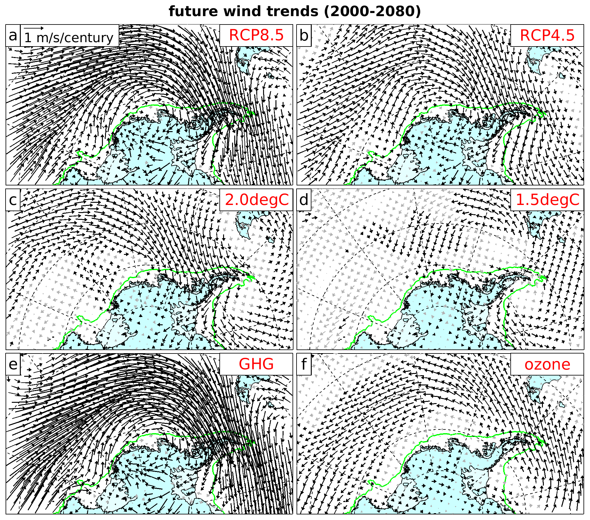
Figure 7Projected wind trends over West Antarctica and their attribution. Panels (a)–(d) show externally forced wind trends in four different forcing scenarios, progressing from the strongest anthropogenic forcing (RCP8.5) to an aggressive emissions mitigation scenario (1.5degC). Panels (e) and (f) show the individual contributions of greenhouse gases and ozone depletion in the RCP8.5 scenario.
High-forcing (RCP8.5) and intermediate-forcing (RCP4.5) scenarios (Fig. 7a and b) feature strong externally forced westerly wind trends over most of the Southern Ocean (Bracegirdle et al., 2020; Goyal et al., 2021) but much weaker trends over the Amundsen Sea shelf (Bracegirdle et al., 2014). Weaker-forcing scenarios are cast in the context of the Paris Agreement, which commits nations to “holding the increase in the global average temperature to well below 2 ∘C above pre-industrial levels and pursuing efforts to limit the temperature increase to 1.5 ∘C”. The 2.0degC scenario substantially reduces future wind trends in this region (Fig. 7c), while 1.5degC eliminates the westerly trends entirely (Fig. 7d). Stabilising global warming removes the Equator-to-pole gradient in temperature trends that drives the westerly wind trends. We speculate that the small remaining wind trends are likely to be very sensitive to the forcing pathway by which temperatures are stabilised. The 1.5degC scenario involves aggressive emissions mitigation and a rapid transition to negative carbon emissions (Sanderson et al., 2017). Historical GHG emissions commit Earth's climate to warming and wind changes for most of the future period studied, so extreme emissions changes are required to reverse these by 2080. Even then, the 1.5degC scenario merely prevents any future trends and does not reverse the historical changes.
As with the historical changes, we may combine ensembles to derive the role of individual external forcings. Figure 7e shows the GHG-forced changes in the RCP8.5 scenario (i.e. LENS minus XGHG). This future GHG response is approximately twice as strong as the historical GHG response (Fig. 2d), with a similar pattern. We cannot directly determine future ozone-forced changes because the fixed-ozone ensemble XOZO terminates in 2005 (Table 1). However, Fig. 7f shows the combined response to all non-GHG external forcings (XGHG minus PIctrl), which we are confident is dominated by the ozone response. For the historical period the non-GHG response closely resembles the ozone response, and in future scenarios the influence of external forcings other than GHGs and ozone (e.g. aerosols) is even weaker (van Vuuren et al., 2011). The future non-GHG response (Fig. 7f) shows a weakening of the westerlies, as expected from the prescribed recovery of stratospheric ozone (Son et al., 2010; Sigmond et al., 2011; Barnes et al., 2014) and in almost exact opposition to the historical ozone-induced changes (Fig. 2f). Thus the models yield the expected result that the future westerly wind trends are driven by GHGs but are partially compensated for by ozone recovery (Thompson et al., 2011). The influence of ozone recovery is expected to be very similar between forcing scenarios (Keeble et al., 2021), so the difference between scenarios in Fig. 7a–d is determined by the extent to which increasing GHGs outweigh this recovery.
The future evolution of the different components of the externally forced wind changes is shown in Fig. 5, which again shows results for RCP8.5. In this strong-forcing scenario, future externally forced trends are of similar magnitude to historical externally forced trends in all regions. Over the deep ocean (Fig. 5b), an increase in the GHG-forced westerly wind trend is compensated for by a negative westerly trend from stratospheric ozone recovery (represented by the non-GHG response). Over the shelf break (Fig. 5d), the ozone-forced trend remains insignificant, but the GHG-forced trend becomes significant in the future period. The recovery of ozone-forced wind trends is focussed earlier in the future period (Keeble et al., 2021), so the overall externally forced trends are weaker during this period and stronger after (Fig. 5a).
Internal variability was an important contributor to wind trends over the Amundsen Sea in the past (Figs. 2 and 5) and could also be important in the future. The evidence suggests that tropical Pacific variability is primarily natural in origin (Stevenson et al., 2012; Cai et al., 2015; Yeh et al., 2018) and cannot be predicted on timescales longer than a few years (Lou et al., 2019). Furthermore, centennial variability in this region does not even appear to follow the recognised modes of tropical Pacific variability (Fig. 1). Therefore, the role of internal variability creates a substantial and potentially irreducible uncertainty in any projection of future wind changes over the Amundsen Sea, particularly in the shelf region.
One way to quantify the influence of internal variability on future wind trends is by considering the ensemble spread in the projections. Figure 8a shows the LENS ensemble-mean trends (i.e. the RCP8.5 externally forced trends in Fig. 7a). Figure 8b quantifies the associated ensemble spread, plotted as the wind trends associated with +1 standard deviation in both zonal and meridional wind trends. This panel shows that there is substantial intra-ensemble variance in the trends, which is evenly spatially distributed and has no obvious preferential wind direction. Figure 8c and e show the future wind trends in two LENS members, chosen manually to illustrate the range of intra-ensemble variance. Both members have strong westerly wind trends overall but differ in their trends over the Amundsen Sea shelf. Figure 8d and f isolate the differing contribution of internal variability in these two members, by subtracting the LENS ensemble mean (the externally forced trends) from both. The internally generated trends have a centre of action north of the Amundsen Sea shelf in both cases, but the trends have either a cyclonic or an anticyclonic orientation depending upon the particular trajectory of internal variability manifested in each simulation.
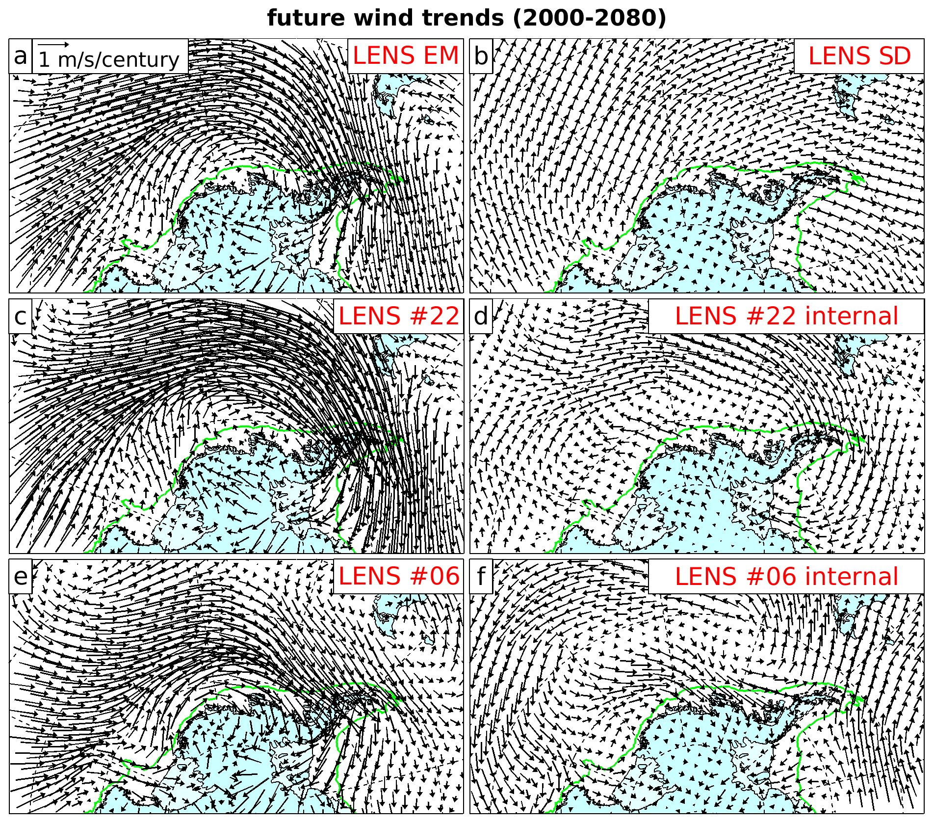
Figure 8Influence of internal variability on projected wind trends over West Antarctica. (a) LENS ensemble-mean wind trends (the RCP8.5 externally forced trend in Fig. 7a). (b) LENS intra-ensemble standard deviation in wind trends, plotted as vectors illustrating one positive standard deviation in both zonal and meridional trends. (c, e) Wind trends in selected illustrative LENS members. (d, f) Deviation of the trends in these selected members from the ensemble-mean trend, illustrating the role of internal climate variability.
Another way to illustrate the potential role of future internal variability is to simply imagine that the historical variability could be repeated or exactly reversed. The advantage of this approach is that our knowledge of the historical variability is constrained by observations. Comparing the historical internally generated trends (Fig. 2c) to the LENS ensemble spread of future internally generated trends (Fig. 8b, d, and f) shows that this is a representative illustration. Following this rationale, Fig. 9 illustrates possible future wind trends that combine forcing-scenario uncertainty with the historically based estimate of future internal variability. This is illustrated simply by adding or subtracting the historical internally generated trends (Fig. 2c) to or from the externally forced trends in the 1.5degC and RCP8.5 forcing scenarios (Fig. 7d and a). It is clear that external forcing and its scenario uncertainty control westerly trends over the deep ocean, while internal variability and its irreducible uncertainty control wind trends over the Amundsen Sea shelf and shelf break.
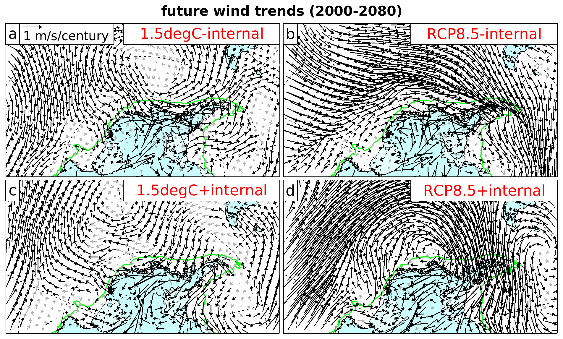
Figure 9Illustrative wind trend projections under different combinations of the external-forcing scenario and a single realisation of internal variability. The columns denote wind trends projected under weak (a, c) and strong (b, d) external forcing, while the rows denote the influence of either subtracting (a, b) or adding (c, d) the wind trends associated with historical internal variability, which is used for illustrative purposes. The projected externally forced wind trends are shown in Fig. 7a and d, while the historical internally generated wind trends are shown in Fig. 2c.
Recent wind anomalies are known to have driven variability in Amundsen Sea ocean conditions and ice-shelf melting that have influenced ice loss from the WAIS (Thoma et al., 2008; Dutrieux et al., 2014; Christianson et al., 2016; Jenkins et al., 2018). Reconstructed winds show that even larger anomalies occurred in the past (Fig. 4), so it is reasonable to assume that these anomalies also induced an ice-sheet response. The reconstructions also reveal interdecadal (∼50 year) variability with an amplitude approximately half that of the annual anomalies. Since ice sheets respond more fully to slower variability (Williams et al., 2012; Snow et al., 2017; Hoffman et al., 2019), it is very likely that these interdecadal anomalies have influenced the WAIS. On centennial timescales, the reconstruction shows that strong westerly wind trends were prevalent over most of the Southern Ocean (Fig. 2). These overall trends were driven by external forcing but partly compensated for by internally generated trends. Over the Amundsen Sea shelf break these contributions cancelled out, leaving no significant overall trend, in contrast to earlier results based on climate models alone (Holland et al., 2019). Over the Amundsen Sea shelf, externally forced trends were absent entirely and an internally generated easterly trend occurred. Where present, the compensating externally forced and internally generated trends are both of similar magnitude to the recent wind variability that we know to be influential on WAIS ice loss. This implies that both the trends and their compensation have been important to the historical evolution of the ice loss.
This evidence suggests a possible narrative for the historical changes in the WAIS. Sediment records show that the ungrounding of Pine Island Glacier commenced in the 1940s (Smith et al., 2017), when the reconstruction shows extreme annual wind events within a multi-decadal period of anomalously anticyclonic winds (Fig. 4). These anomalies were all internally generated (Fig. 5) and partly associated with tropical Pacific variability (Fig. 6). By the mid-1970s the ice shelf was fully ungrounded (Jenkins et al., 2010; Smith et al., 2017), following a period of retreat that was probably enhanced by ice and ocean feedbacks (De Rydt et al., 2014; De Rydt and Gudmundsson, 2016). The triggering internal variability had reversed by the 1960s, but by then the GHG-forced wind anomalies had appeared (Fig. 5). Perhaps, without external forcing, the reversed internal variability might have allowed the ice to re-advance and fully re-ground on the ridge. In the 1980s the external forcing increased further with ever-increasing GHGs and the onset of ozone depletion, and the internally generated anomalies became anticyclonic again. The wind changes resulting from these anthropogenic and natural drivers were of approximately equal magnitude, suggesting that a combination of these factors drove the current period of rapid, accelerating ice loss (Mouginot et al., 2014; Konrad et al., 2017; Shepherd et al., 2019).
While much remains uncertain, this narrative can simultaneously satisfy lines of evidence from palaeoclimate proxies, Amundsen Sea sediment records, ocean observations, climate model simulations, and the satellite record of ice loss. Importantly, it also resolves an apparent paradox. The WAIS is thought to have been broadly stable for ∼10 000 years in this region (Larter et al., 2014) before the current retreat was initiated in the 1940s (Smith et al., 2017) by internal climate variability (Figs. 4 and 5). However, by definition it is very unlikely that this natural variability was unprecedented in the previous millennia, so why did it trigger an exceptional ice retreat? One way to resolve this apparent paradox is if the initial retreat was natural but the subsequent failure of the ice sheet to re-advance was influenced by anthropogenic forcing. Perhaps the ice sheet experienced several short-lived retreats during the last few millennia, from which it recovered, but it failed to recover from the 1940s retreat because external forcing over-rode the subsequent reversal of the natural climatic variability (Figs. 4 and 5). We emphasise that this is not the only possible resolution of this “paradox”, however. For example, if some slow background change had occurred over the millennia, such as a reduction in surface accumulation, this could have gradually reduced the stability of the glaciers in the region. The 1940s variability may then have been able to destabilise the glaciers simply because they were more vulnerable.
Turning to the future changes, 2000–2080, we again find that both external forcing and internal variability are of comparable importance. Remarkably, the choice of emissions scenario is important to wind trends everywhere apart from the Amundsen Sea shelf. On the shelf, future wind trends are dictated solely by internal variability, while over the deep ocean the external forcing plays a larger role. Under an aggressive emissions mitigation scenario that limits global warming to 1.5 ∘C, there are no externally forced zonal wind trends during the future period. Under high-emissions (RCP8.5) or even intermediate-emissions (RCP4.5) scenarios, future externally forced zonal wind trends approximately equal the historical externally forced trends. Thus, future forcing will range between maintaining the existing externally forced changes (1.5degC scenario) and approximately doubling them (RCP8.5). To the extent that ice loss from the WAIS is driven by externally forced wind trends, that part of the ice loss cannot be reversed before 2080 and will probably increase.
Internally generated trends provided an important compensation of the externally forced trends during the historical period and could be similarly influential in the future. If externally forced trends were eliminated in the future, internally generated trends could dictate the future trajectory of the WAIS (Fig. 9). On the other hand, if higher-emissions scenarios are followed, internal variability may do little more than influence the timing and rate of the ongoing ice loss. Minimising future wind-driven WAIS ice loss will require strong emissions mitigation, but the uncontrollable future influence of internal climate variability could be equally important.
There are, of course, many caveats to these findings. This study considers a single palaeoclimate reconstruction and climate model and is therefore subject to the structural uncertainty inherent in these sources (see Sect. 2). The study does not investigate seasonal variations due to the annual resolution of the reconstruction. This is an important limitation because there are strong seasonal variations in the impacts of both external forcing (e.g. ozone depletion; Thompson et al., 2011) and internal variability (e.g. the tropical Pacific teleconnection; Ding et al., 2012). The study also only considers wind forcing of changes in the ocean, but of course thermodynamic forcings may also be important, and ice-sheet dynamics and ice–ocean feedbacks certainly modulate the ice response to any climatic forcing. Finally, we require further information about the oceanographic implications of the wind changes described in this study. Based on our conclusions, anthropogenic forcings are expected to be most influential over the deep ocean and in summer, while internal variability should be more influential on the shelf and in winter. Therefore, to derive the relative influence of external forcing, we urgently need information on the regional and seasonal influence of winds on ocean properties and ice melting. Despite all these important limitations on the interpretation of our results, we emphasise that all of the wind changes discussed are comparable in magnitude to the recent variability, which we know to have been influential over WAIS ice loss.
Over recent decades, wind-driven variability in the Amundsen Sea has regulated ocean melting of the WAIS. This study combines palaeoclimate reconstructions and climate model simulations to understand wind changes over the Amundsen Sea during the 20th and 21st centuries.
By combining these two sources of information, we are able to separate natural, internally generated wind changes from anthropogenic, externally forced changes. Both are important. Firstly, internal variability on interannual and interdecadal timescales has a magnitude comparable to centennial trends. Secondly, the centennial trends themselves are generated by comparable contributions from external forcing and internal variability. To the extent that wind-driven changes control WAIS ice loss, both external forcing and internal variability are important contributors.
Historical wind trends (1920–2000) have two components: acceleration of the westerlies over the deep ocean, forced by GHGs and ozone depletion, and a cyclonic trend pattern centred over the Amundsen Sea that is largely internally generated. Over most of the region, internally generated easterly wind trends compensate for externally forced westerly wind trends. Historical winds also exhibit strong variability, linked to the tropical Pacific, including both strong interannual anomalies and interdecadal variability that reverses on a timescale of approximately 50 years.
This evidence suggests a possible narrative for historical ice loss from the WAIS. Ice retreat was triggered in the 1940s by internal variability. This variability had reversed by the 1960s, but by then GHG-forced wind changes had started to increase. Perhaps without external forcing, the reversed internal variability may have allowed the ice sheet to re-advance. In the 1980s the external forcing increased further with the onset of ozone depletion, and the internal variability changed sign again. These changes drove the current period of rapid, accelerating ice loss. There remain many uncertainties with this narrative, but it resolves an apparent paradox whereby the present ice loss appears to have been triggered naturally but involves a retreat unprecedented in millennia. Perhaps short-lived retreats have occurred several times in the past, but the ice always re-advanced in the absence of anthropogenic forcing.
During the future period (2000–2080), westerly wind trends driven by GHGs are partially offset by stratospheric ozone recovery. Wind trends are responsive to forcing scenario, but only extreme emissions mitigation consistent with a Paris Agreement target of 1.5 ∘C warming above pre-industrial levels is able to prevent further wind trends during this period (let alone offset historical trends). The choice of anthropogenic forcing scenario is most influential on westerly trends over the deep ocean, while the irreducible uncertainty associated with internally generated variability is strongest on the Amundsen Sea shelf. Minimal future wind-driven WAIS ice loss will require strong emissions mitigation and a favourable evolution of natural climate variability.
The CESM1 simulations are available at the NCAR Climate Data Gateway (https://www.earthsystemgrid.org/, NCAR, 2021), as detailed in the references in Table 1. The palaeoclimate reconstructions generated in the study by O'Connor et al. (2021a) are archived at Zenodo (https://doi.org/10.5281/zenodo.5507607, O'Connor et al., 2021b).
PRH and GKO'C conceived the study and led the data processing. All authors discussed the results and implications and collaborated on writing the manuscript at all stages.
The contact author has declared that none of the authors has any competing interests.
Publisher's note: Copernicus Publications remains neutral with regard to jurisdictional claims in published maps and institutional affiliations.
We are grateful to the originators of the many open-access datasets synthesised in this study, particularly the PAGES2k palaeoclimate proxy database and the CESM1 climate model simulations. We thank all the scientists, software engineers, and administrators who contributed to the development of CESM1.
This publication was supported by PROTECT. This project has received funding from the European Union's Horizon 2020 research and innovation programme under grant agreement no. 869304, PROTECT contribution number 52. Gemma K. O'Connor was supported by the NSF Graduate Research Fellowship Program. Kaitlin A. Naughten was supported by award NE/S011994/1. David P. Schneider was partially supported by NSF grant 1952199 and partially supported by the National Center for Atmospheric Research (NCAR), which is a major facility sponsored by the NSF under cooperative agreement no. 1852977. CESM1 is primarily supported by the National Science Foundation (NSF).
This paper was edited by Michiel van den Broeke and reviewed by two anonymous referees.
Agosta, C., Fettweis, X., and Datta, R.: Evaluation of the CMIP5 models in the aim of regional modelling of the Antarctic surface mass balance, The Cryosphere, 9, 2311–2321, https://doi.org/10.5194/tc-9-2311-2015, 2015.
Arblaster, J. M. and Meehl, G. A.: Contributions of external forcings to Southern Annular Mode trends, J. Climate, 19, 2896–2905, https://doi.org/10.1175/Jcli3774.1, 2006.
Barnes, E. A., Barnes, N. W., and Polvani, L. M.: Delayed Southern Hemisphere Climate Change Induced by Stratospheric Ozone Recovery, as Projected by the CMIP5 Models, J. Climate, 27, 852–867, https://doi.org/10.1175/Jcli-D-13-00246.1, 2014.
Barthel, A., Agosta, C., Little, C. M., Hattermann, T., Jourdain, N. C., Goelzer, H., Nowicki, S., Seroussi, H., Straneo, F., and Bracegirdle, T. J.: CMIP5 model selection for ISMIP6 ice sheet model forcing: Greenland and Antarctica, The Cryosphere, 14, 855–879, https://doi.org/10.5194/tc-14-855-2020, 2020.
Bett, D. T., Holland, P. R., Naveira Garabato, A. C., Jenkins, A., Dutrieux, P., Kimura, S., and Fleming, A.: The impact of the Amundsen Sea freshwater balance on ocean melting of the West Antarctic Ice Sheet, J. Geophys. Res., 125, e2020JC016305, https://doi.org/10.1029/2020JC016305, 2020.
Bracegirdle, T. J., Turner, J., Hosking, J. S., and Phillips, T.: Sources of uncertainty in projections of 21st century westerly wind changes over the Amundsen Sea, West Antarctica, in CMIP5 climate models, Clim. Dynam., 43, 2093–2104, https://doi.org/10.1007/s00382-013-2032-1, 2014.
Bracegirdle, T. J., Krinner, G., Tonelli, M., Haumann, F. A., Naughten, K. A., Rackow, T., Roach, L. A., and Wainer, I.: Twenty first century changes in Antarctic and Southern Ocean surface climate in CMIP6, Atmos. Sci. Lett., 21, e984, https://doi.org/10.1002/asl.984, 2020.
Cai, W. J., Santoso, A., Wang, G. J., Yeh, S. W., An, S. I., Cobb, K. M., Collins, M., Guilyardi, E., Jin, F. F., Kug, J. S., Lengaigne, M., McPhaden, M. J., Takahashi, K., Timmermann, A., Vecchi, G., Watanabe, M., and Wu, L. X.: ENSO and greenhouse warming, Nat. Clim. Change, 5, 849–859, https://doi.org/10.1038/Nclimate2743, 2015.
Christianson, K., Bushuk, M., Dutrieux, P., Parizek, B. R., Joughin, I. R., Alley, R. B., Shean, D. E., Abrahamsen, E. P., Anandakrishnan, S., Heywood, K. J., Kim, T. W., Lee, S. H., Nicholls, K., Stanton, T., Truffer, M., Webber, B. G. M., Jenkins, A., Jacobs, S., Bindschadler, R., and Holland, D. M.: Sensitivity of Pine Island Glacier to observed ocean forcing, Geophys. Res. Lett., 43, 10817–10825, https://doi.org/10.1002/2016gl070500, 2016.
Ciasto, L. M. and Thompson, D. W. J.: Observations of large-scale ocean-atmosphere interaction in the Southern Hmisphere, J. Climate, 21, 1244–1259, https://doi.org/10.1175/2007JCLI1809.1, 2008.
Dalaiden, Q., Goosse, H., Rezsöhazy, J., and Thomas, E. R.: Reconstructing atmospheric circulation and sea-ice extent in the West Antarctic over the past 200 years using data assimilation, Clim. Dynam., 57, 3479–3503, https://doi.org/10.1007/s00382-021-05879-6, 2021.
Dalaiden, Q., Schurer, A. P., Kirchmeier-Young, M. C., Goosse, H., and Hegerl, G. C.: West Antarctic surface climate changes since the mid-20th century driven by anthropogenic forcing, Geophys. Res. Lett., 49, e2022GL099543, https://doi.org/10.1029/2022GL099543, 2022.
De Rydt, J. and Gudmundsson, G. H.: Coupled ice shelf-ocean modeling and complex grounding line retreat from a seabed ridge, J. Geophys. Res.-Earth, 121, 865–880, https://doi.org/10.1002/2015jf003791, 2016.
De Rydt, J., Holland, P. R., Dutrieux, P., and Jenkins, A.: Geometric and oceanographic controls on melting beneath Pine Island Glacier, J. Geophys. Res., 119, 2420–2438, https://doi.org/10.1002/2013JC009513, 2014.
De Rydt, J., Reese, R., Paolo, F. S., and Gudmundsson, G. H.: Drivers of Pine Island Glacier speed-up between 1996 and 2016, The Cryosphere, 15, 113–132, https://doi.org/10.5194/tc-15-113-2021, 2021.
Deser, C., Phillips, A. S., Simpson, I. R., Rosenbloom, N., Coleman, D., Lehner, F., Pendergrass, A. G., DiNezio, P., and Stevenson, S.: Isolating the Evolving Contributions of Anthropogenic Aerosols and Greenhouse Gases: A New CESM1 Large Ensemble Community Resource, J. Climate, 33, 7835–7858, https://doi.org/10.1175/JCLI-D-20-0123.1, 2020.
Ding, Q., Steig, E. J., Battisti, D. S., and Wallace, J. M.: Influence of the Tropics on the Southern Annular Mode, J. Climate, 25, 6330–6348, https://doi.org/10.1175/JCLI-D-11-00523.1, 2012.
Ding, Q. H., Steig, E. J., Battisti, D. S., and Kuttel, M.: Winter warming in West Antarctica caused by central tropical Pacific warming, Nat. Geosci., 4, 398–403, https://doi.org/10.1038/NGEO1129, 2011.
Dutrieux, P., De Rydt, J., Jenkins, A., Holland, P. R., Ha, H. K., Lee, S. H., Steig, E. J., Ding, Q. H., Abrahamsen, E. P., and Schroder, M.: Strong Sensitivity of Pine Island Ice-Shelf Melting to Climatic Variability, Science, 343, 174–178, https://doi.org/10.1126/science.1244341, 2014.
England, M. R., Polvani, L. M., Smith, K. L., Landrum, L., and Holland, M. M.: Robust response of the Amundsen Sea Low to stratospheric ozone depletion, Geophys. Res. Lett., 43, 8207–8213, https://doi.org/10.1002/2016GL070055, 2016.
Favier, L., Durand, G., Cornford, S. L., Gudmundsson, G. H., Gagliardini, O., Gillet-Chaulet, F., Zwinger, T., Payne, A. J., and Le Brocq, A. M.: Retreat of Pine Island Glacier controlled by marine ice-sheet instability, Nat. Clim. Change, 4, 117–121, https://doi.org/10.1038/nclimate2094, 2014.
Fogt, R. L., Schneider, D. P., Goergens, C. A., Jones, J. M., Clark, L. N., and Garberoglio, M. J.: Seasonal Antarctic pressure variability during the twentieth century from spatially complete reconstructions and CAM5 simulations, Clim. Dynam., 53, 1435–1452, https://doi.org/10.1007/s00382-019-04674-8, 2019.
Gillett, N. P., Fyfe, J. C., and Parker, D. E.: Attribution of observed sea level pressure trends to greenhouse gas, aerosol, and ozone changes, Geophys. Res. Lett., 40, 2302–2306, https://doi.org/10.1002/grl.50500, 2013.
Goyal, R., Gupda, A. S., Jucker, M., and England, M. H.: Historical and projected changes in the Southern Hemisphere surface westerlies, Geophys. Res. Lett., 48, e2020GL090849, https://doi.org/10.1029/2020GL090849, 2021.
Hakim, G. J., Emile-Geay, J., Steig, E. J., Noone, D., Anderson, D. M., Tardif, R., Steiger, N., and Perkins, W. A.: The last millenium climate reanalysis project: Framework and first results, J. Geophys. Res.-Atmos., 121, 6745–6764, https://doi.org/10.1002/2016JD024751, 2016.
Harvey, B. J., Shaffrey, L. C., and Woollings, T. J.: Equator-to-pole temperature differences and the extra-tropical storm track responses of the CMIP5 climate models, Clim. Dynam., 43, 1171–1182, https://doi.org/10.1007/s00382-013-1883-9, 2014.
Henley, B. J., Gergis, J., Karoly, D. J., Power, S., Kennedy, J., and Folland, C. K.: A Tripole Index for the Interdecadal Pacific Oscillation, Clim. Dynam., 45, 3077–3090, https://doi.org/10.1007/s00382-015-2525-1, 2015.
Hersbach, H.: The ERA5 global reanalysis, Q. J. Roy. Meteor. Soc., 146, 1999–2049, https://doi.org/10.1002/qj.3803, 2020.
Hines, K. M., Bromwich, D. H., and Marshall, G. J.: Artificial Surface Pressure Trends in the NCEP–NCAR Reanalysis over the Southern Ocean and Antarctica, J. Climate, 13, 3940–3952, 2000.
Hoffman, M. J., Asay-Davis, X., Price, S. F., Fyke, J., and Perego, M.: Effect of Subshelf Melt Variability on Sea Level Rise Contribution From Thwaites Glacier, Antarctica, J. Geophys. Res.-Earth, 124, 2798–2822, https://doi.org/10.1029/2019JF005155, 2019.
Holland, P. R., Bracegirdle, T. J., Dutrieux, P., Jenkins, A., and Steig, E. J.: West Antarctic ice loss influenced by internal climate variability and anthropogenic forcing, Nat. Geosci., 12, 718–724, https://doi.org/10.1038/s41561-019-0420-9, 2019.
IPCC: IPCC Special Report on the Ocean and Cryosphere in a Changing Climate, edited by: Pörtner, H.-O., Roberts, D. C., Masson-Delmotte, V., Zhai, P., Tignor, M., Poloczanska, E., Mintenbeck, K., Alegría, A., Nicolai, M., Okem, A., Petzold, J., Rama, B., and Weyer, N. M., Cambridge University Press, Cambridge, UK and New York, NY, USA, 755 pp., https://doi.org/10.1017/9781009157964, 2019.
Jenkins, A., Dutrieux, P., Jacobs, S. S., McPhail, S. D., Perrett, J. R., Webb, A. T., and White, D.: Observations beneath Pine Island Glacier in West Antarctica and implications for its retreat, Nat. Geosci., 3, 468–472, https://doi.org/10.1038/Ngeo890, 2010.
Jenkins, A., Shoosmith, D., Dutrieux, P., Jacobs, S., Kim, T. W., Lee, S. H., Ha, H. K., and Stammerjohn, S.: West Antarctic Ice Sheet retreat in the Amundsen Sea driven by decadal oceanic variability, Nat. Geosci., 11, 733–738, https://doi.org/10.1038/s41561-018-0207-4, 2018.
Karoly, D.: Southern Hemisphere Circulation Features Associated with El Niño-Southern Oscillation Events, J. Climate, 2, 1239–1252, 1989.
Kay, J. E., Deser, C., Phillips, A., Mai, A., Hannay, C., Strand, G., Arblaster, J. M., Bates, S. C., Danabasoglu, G., Edwards, J., Holland, M., Kushner, P., Lamarque, J. F., Lawrence, D., Lindsay, K., Middleton, A., Munoz, E., Neale, R., Oleson, K., Polvani, L., and Vertenstein, M.: The Community Earth System Model (CESM) Large Ensemble Project: A Community Resource for Studying Climate Change in the Presence of Internal Climate Variability, B. Am. Meteorol. Soc., 96, 1333–1349, https://doi.org/10.1175/Bams-D-13-00255.1, 2015.
Kay, J. E., Wall, C., Yettella, V., Medeiros, B., Hannay, C., Caldwell, P., and Bitz, C.: Global climate impacts of fixing the Southern Ocean shortwave radiation bias in the Community Earth System Model, J. Climate, 29, 4617–4636, https://doi.org/10.1175/JCLI-D-15-0358.1, 2016.
Keeble, J., Hassler, B., Banerjee, A., Checa-Garcia, R., Chiodo, G., Davis, S., Eyring, V., Griffiths, P. T., Morgenstern, O., Nowack, P., Zeng, G., Zhang, J., Bodeker, G., Burrows, S., Cameron-Smith, P., Cugnet, D., Danek, C., Deushi, M., Horowitz, L. W., Kubin, A., Li, L., Lohmann, G., Michou, M., Mills, M. J., Nabat, P., Olivié, D., Park, S., Seland, Ø., Stoll, J., Wieners, K.-H., and Wu, T.: Evaluating stratospheric ozone and water vapour changes in CMIP6 models from 1850 to 2100, Atmos. Chem. Phys., 21, 5015–5061, https://doi.org/10.5194/acp-21-5015-2021, 2021.
Kimura, S., Jenkins, A., Regan, H., Holland, P. R., Assmann, K. M., Whitt, D. B., Van Wessem, M., van de Berg, W. J., Reijmer, C. H., and Dutrieux, P.: Oceanographic Controls on the Variability of Ice-Shelf Basal Melting and Circulation of Glacial Meltwater in the Amundsen Sea Embayment, Antarctica, J. Geophys. Res., 122, 10131–10155, https://doi.org/10.1002/2017jc012926, 2017.
Konrad, H., Gilbert, L., Cornford, S. L., Payne, A. J., Hogg, A., Muir, A., and Shepherd, A.: Uneven onset and pace of ice-dynamical imbalance in the Amundsen Sea Embayment, West Antarctica, Geophys. Res. Lett., 44, 910–918, https://doi.org/10.1002/2016GL070733, 2017.
Lachlan-Cope, T. and Connolley, W.: Teleconnections between the tropical Pacific and the Amundsen-Bellinghausens sea: Role of the El Niño Southern Oscillation, J. Geophys. Res.-Atmos., 111, D23101, https://doi.org/10.1029/2005jd006386, 2006.
Larter, R. D., Anderson, J. B., Graham, A. G. C., Gohl, K., Hillenbrand, C.-D., Jakobsson, M., Johnson, J. S., Kuhn, G., Nitsche, F., Smith, J. A., Witus, A. E., Bentley, M. J., Dowdeswell, J. A., Ehrmann, W., Klages, J. P., Lindow, J., O Cofaigh, C., and Spiegel, C.: Reconstruction of changes in the Amundsen Sea and Bellingshausen Sea sector of the West Antarctic Ice Sheet since the Last Glacial Maximum, Quaternary Sci. Rev., 100, 55–86, https://doi.org/10.1016/j.quascirev.2013.10.016, 2014.
Lenaerts, J. T. M., Vizcaino, M., Fyke, J., van Kampenhout, L., and van den Broeke, M. R.: Present-day and future Antarctic ice sheet climate and surface mass balance in the Community Earth System Model, Clim. Dynam., 47, 1367–1381, https://doi.org/10.1007/s00382-015-2907-4, 2016.
Lhermitte, S., Sun, S., Shuman, C., Wouters, B., Pattyn, F., Wuite, J., Berthier, E., and Nagler, T.: Damage accelerates ice shelf instability and mass loss in Amundsen Sea Embayment, P. Natl. Acad. Sci. USA, 117, 24735–24741, https://doi.org/10.1073/pnas.1912890117, 2020.
Lou, J., Holbrook, N. J., and O'Kane, T. J.: South Pacific Decadal Climate Variability and Potential Predictability, J. Climate, 32, 6051–6069, https://doi.org/10.1175/JCLI-D-18-0249.1, 2019.
Marshall, G. J.: Trends in the Southern Annular Mode from observations and reanalyses, J. Climate, 16, 4134–4143, 2003.
Marshall, G. J., Fogt, R. L., Turner, J., and Clem, K. R.: Can current reanalyses accurately portray changes in Southern Annular Mode structure prior to 1979?, Clim. Dynam., 59, 3717–3740, https://doi.org/10.1007/s00382-022-06292-3, 2022.
Meehl, G. A., Arblaster, J. M., Bitz, C. M., Chung, C. T. Y., and Teng, H. Y.: Antarctic sea-ice expansion between 2000 and 2014 driven by tropical Pacific decadal climate variability, Nat. Geosci., 9, 590–595, https://doi.org/10.1038/ngeo2751, 2016.
Mouginot, J., Rignot, E., and Scheuchl, B.: Sustained increase in ice discharge from the Amundsen Sea Embayment, West Antarctica, from 1973 to 2013, Geophys. Res. Lett., 41, 1576–1584, https://doi.org/10.1002/2013gl059069, 2014.
Naughten, K. A., Holland, P. R., Dutrieux, P., Kimura, S., Bett, D. T., and Jenkins, A.: Simulated twentieth-century ocean warming in the Amundsen Sea, West Antarctica, Geophys. Res. Lett., 49, e2021GL094566, https://doi.org/10.1029/2021GL094566, 2022.
NCAR: Climate Data Gateway, https://www.earthsystemgrid.org/, last access: 21 December 2022.
Newman, M., Alexander, M. A., Ault, T. R., Cobb, K. M., Deser, C., Di Lorenzo, E., Mantua, N. J., Miller, A. J., Minobe, S., Nakamura, H., Schneider, N., Vimont, D. J., Phillips, A. S., Scott, J. D., and Smith, C. A.: The Pacific Decadal Oscillation, Revisited, J. Climate, 29, 4399–4427, https://doi.org/10.1175/Jcli-D-15-0508.1, 2016.
O'Connor, G. K., Steig, E. J., and Hakim, G. J.: Strengthening Southern Hemisphere westerlies and Amundsen Sea Low deepening over the 20th century revealed by proxy-data assimilation, Geophys. Res. Lett., 48, e2021GL095999, https://doi.org/10.1029/2021GL095999, 2021a.
O'Connor, G. K., Steig, E. J., and Hakim, G. J.: Southern Hemisphere winds, pressure, and temperature over the 20th century from proxy-data assimilation, Zenodo [data set], https://doi.org/10.5281/zenodo.5507607, 2021b.
PAGES2k: A global multiproxy database for temperature reconstructions of the Common Era, Scientific Data, 4, 170088, https://doi.org/10.1038/sdata.2017.88, 2017.
Paolo, F. S., Fricker, H. A., and Padman, L.: Volume loss from Antarctic ice shelves is accelerating, Science, 348, 327–331, https://doi.org/10.1126/science.aaa0940, 2015.
Purich, A., England, M. H., Cai, W., Chikamoto, Y., Timmermann, A., Fyfe, J. C., Frankcombe, L., Meehl, G. A., and Arblaster, J. M.: Tropical Pacific SST Drivers of Recent Antarctic Sea Ice Trends, J. Climate, 29, 8931–8948, https://doi.org/10.1175/Jcli-D-16-0440.1, 2016.
Raphael, M. N., Marshall, G. J., Turner, J., Fogt, R. L., Schneider, D., Dixon, D. A., Hosking, J. S., Jones, J. M., and Hobbs, W. R.: The Amundsen Sea Low: Variability, Change, and Impact on Antarctic Climate, B. Am. Meteorol. Soc., 97, 111–121, https://doi.org/10.1175/Bams-D-14-00018.1, 2016.
Rayner, N. A., Parker, D. E., Horton, E. B., Folland, C. K., Alexander, L. V., Rowell, D. P., Kent, E. C., and Kaplan, A.: Global analyses of sea surface temperature, sea ice, and night marine air temperature since the late nineteenth century, J. Geophys. Res.-Atmos., 108, 4407, https://doi.org/10.1029/2002jd002670, 2003.
Rignot, E., Mouginot, J., Morlighem, M., Seroussi, H., and Scheuchl, B.: Widespread, rapid grounding line retreat of Pine Island, Thwaites, Smith, and Kohler glaciers, West Antarctica, from 1992 to 2011, Geophys. Res. Lett., 41, 3502–3509, https://doi.org/10.1002/2014GL060140, 2014.
Sanderson, B. M., Xu, Y., Tebaldi, C., Wehner, M., O'Neill, B., Jahn, A., Pendergrass, A. G., Lehner, F., Strand, W. G., Lin, L., Knutti, R., and Lamarque, J. F.: Community climate simulations to assess avoided impacts in 1.5 and 2 ∘C futures, Earth Syst. Dynam., 8, 827–847, https://doi.org/10.5194/esd-8-827-2017, 2017.
Sanderson, B. M., Oleson, K. W., Strand, W. G., Lehner, F., and O'Neill, B. C.: A new ensemble of GCM simulations to assess avoided impacts in a climate mitigation scenario, Climatic Change, 146, 303–318, https://doi.org/10.1007/s10584-015-1567-z, 2018.
Schneider, D. P. and Deser, C.: Tropically driven and externally forced patterns of Antarctic sea ice change: reconciling observed and modeled trends, Clim. Dynam., 50, 4599–4618, https://doi.org/10.1007/s00382-017-3893-5, 2018.
Schneider, D. P. and Steig, E. J.: Ice cores record significant 1940s Antarctic warmth related to tropical climate variability, P. Natl. Acad. Sci. USA, 105, 12154–12158, https://doi.org/10.1073/pnas.0803627105, 2008.
Shaw, T. A.: Mechanisms of Future Predicted Changes in the Zonal Mean Mid-Latitude Circulation, Current Climate Change Reports, 5, 345–357, https://doi.org/10.1007/s40641-019-00145-8, 2019.
Shepherd, A., Wingham, D., and Rignot, E.: Warm ocean is eroding West Antarctic Ice Sheet, Geophys. Res. Lett., 31, L23402, https://doi.org/10.1029/2004gl021106, 2004.
Shepherd, A., Gilbert, L., Muir, A. S., Konrad, H., McMillan, M., Slater, T., Briggs, K. H., Sundal, A. V., Hogg, A. E., and Engdahl, M. E.: Trends in Antarctic Ice Sheet Elevation and Mass, Geophys. Res. Lett., 46, 8174–8183, https://doi.org/10.1029/2019gl082182, 2019.
Sigmond, M., Reader, M. C., Fyfe, J. C., and Gillett, N. P.: Drivers of past and future Southern Ocean change: Stratospheric ozone versus greenhouse gas impacts, Geophys. Res. Lett., 38, L12601, https://doi.org/10.1029/2011GL047120, 2011.
Smith, J. A., Andersen, T. J., Shortt, M., Gaffney, A. M., Truffer, M., Stanton, T. P., Bindschadler, R., Dutrieux, P., Jenkins, A., Hillenbrand, C. D., Ehrmann, W., Corr, H. F. J., Farley, N., Crowhurst, S., and Vaughan, D. G.: Sub-ice-shelf sediments record history of twentieth-century retreat of Pine Island Glacier, Nature, 549, 292–292, https://doi.org/10.1038/nature23650, 2017.
Snow, K., Goldberg, D. N., Holland, P. R., Jordan, J. R., Arthern, R. J., and Jenkins, A.: The Response of Ice Sheets to Climate Variability, Geophys. Res. Lett., 44, 11878–11885, https://doi.org/10.1002/2017gl075745, 2017.
Son, S.-W., Gerber, E. P., Perlwitz, J., Polvani, L. M., Gillett, N. P., Seo, K.-H., Eyring, V., Shepherd, T. G., Waugh, D., Akiyoshi, H., Austin, J., Baumgaertner, A., Bekki, S., Braesicke, P., Brühl, C., Butchart, N., Chipperfield, M. P., Cugnet, D., Dameris, M., Dhomse, S., Frith, S., Garny, H., Garcia, R., Hardiman, S. C., Jöckel, P., Lamarque, J. F., Mancini, E., Marchand, M., Michou, M., Nakamura, T. and Morgenstern, O., Pitari, G., Plummer, D. A., Pyle, J., Rozanov, E., Scinocca, J. F., Shibata, K., Smale, D., Teyssèdre, H., Tian, W., and Yamashita, Y.: Impact of stratospheric ozone on Southern Hemisphere circulation change: A multimodel assessment, J. Geophys. Res.-Atmos., 115, D00M07, https://doi.org/10.1029/2010JD014271, 2010.
Steig, E. J., Ding, Q., Battisti, D. S., and Jenkins, A.: Tropical forcing of Circumpolar Deep Water Inflow and outlet glacier thinning in the Amundsen Sea Embayment, West Antarctica, Ann. Glaciol., 53, 19–28, https://doi.org/10.3189/2012AoG60A110, 2012.
Steig, E. J., Ding, Q. H., White, J. W. C., Kuttel, M., Rupper, S. B., Neumann, T. A., Neff, P. D., Gallant, A. J. E., Mayewski, P. A., Taylor, K. C., Hoffmann, G., Dixon, D. A., Schoenemann, S. W., Markle, B. R., Fudge, T. J., Schneider, D. P., Schauer, A. J., Teel, R. P., Vaughn, B. H., Burgener, L., Williams, J., and Korotkikh, E.: Recent climate and ice-sheet changes in West Antarctica compared with the past 2000 years, Nat. Geosci., 6, 372–375, https://doi.org/10.1038/Ngeo1778, 2013.
Stevenson, S., Fox-Kemper, B., Jochum, M., Neale, R., Deser, C., and Meehl, G.: Will There Be a Significant Change to El Niño in the Twenty-First Century?, J. Climate, 25, 2129–2145, https://doi.org/10.1175/JCLI-D-11-00252.1, 2012.
Tardif, R., Hakim, G. J., Perkins, W. A., Horlick, K. A., Erb, M. P., Emile-Geay, J., Anderson, D. M., Steig, E. J., and Noone, D.: Last Millennium Reanalysis with an expanded proxy database and seasonal proxy modeling, Clim. Past, 15, 1251–1273, https://doi.org/10.5194/cp-15-1251-2019, 2019.
Thoma, M., Jenkins, A., Holland, D., and Jacobs, S.: Modelling Circumpolar Deep Water intrusions on the Amundsen Sea continental shelf, Antarctica, Geophys. Res. Lett., 35, L18602, https://doi.org/10.1029/2008gl034939, 2008.
Thompson, D. W. J., Solomon, S., Kushner, P. J., England, M. H., Grise, K. M., and Karoly, D. J.: Signatures of the Antarctic ozone hole in Southern Hemisphere surface climate change, Nat. Geosci., 4, 741–749, https://doi.org/10.1038/Ngeo1296, 2011.
van Vuuren, D. P., Edmonds, J., Kainuma, M., Riahi, K., Thomson, A., Hibbard, K., Hurtt, G. C., Kram, T., Krey, V., Lamarque, J.-F., Masui, T., Meinshausen, M., Nakicenovic, N., Smith, S. J., and Rose, S. K.: The representative concentration pathways: an overview, Climatic Change, 109, 5–31, https://doi.org/10.1007/s10584-011-0148-z, 2011.
Williams, C. R., Hindmarsh, R. C. A., and Arthern, R. J.: Frequency response of ice streams, P. R. Soc. A, 468, 3285–3310, https://doi.org/10.1098/rspa.2012.0180, 2012.
Yeh, S. W., Cai, W. J., Min, S. K., McPhaden, M. J., Dommenget, D., Dewitte, B., Collins, M., Ashok, K., An, S. I., Yim, B. Y., and Kug, J. S.: ENSO Atmospheric Teleconnections and Their Response to Greenhouse Gas Forcing, Rev. Geophys., 56, 185–206, https://doi.org/10.1002/2017rg000568, 2018.