Simulating the current and future northern limit of permafrost on the Qinghai–Tibet Plateau

Permafrost has been warming and thawing globally, with subsequent effects on the climate, hydrology, and the ecosystem. However, the permafrost thermal state variation in the northern lower limit of the permafrost zone (Xidatan) on the Qinghai–Tibet Plateau (QTP) is unclear. This study attempts to explore the changes and variability in this permafrost using historical (1970–2019) and future projection datasets from remote-sensing-based land surface temperature product (LST) and climate projections from Earth system model (ESM) outputs of the Coupled Model Intercomparison Project Phase 5 and 6 (CMIP5, CMIP6). Our model considers phase-change processes of soil pore water, thermal-property differences between frozen and unfrozen soil, geothermal flux flow, and the ground ice effect. Our model can consistently reproduce the vertical ground temperature profiles and active layer thickness (ALT), recognizing permafrost boundaries, and capture the evolution of the permafrost thermal regime. The spatial distribution of permafrost and its thermal conditions over the study area were controlled by elevation with a strong influence of slope orientation. From 1970 to 2019, the mean annual ground temperature (MAGT) in the region warmed by 0.49 ^∘C in the continuous permafrost zone and 0.40 ^∘C in the discontinuous permafrost zone. The lowest elevation of the permafrost boundary (on the north-facing slopes) rose approximately 47 m, and the northern boundary of discontinuous permafrost retreated southwards by approximately 1–2 km, while the lowest elevation of the permafrost boundary remained unchanged for the continuous permafrost zone. The warming rate in MAGT is projected to be more pronounced under shared socioeconomic pathways (SSPs) than under representative concentration pathways (RCPs), but there are no distinct discrepancies in the areal extent of the continuous and discontinuous permafrost and seasonally frozen ground among SSP and RCP scenarios. This study highlights the slow delaying process of the response of permafrost in the QTP to a warming climate, especially in terms of the areal extent of permafrost distribution.

1 Introduction

Permafrost is one of the crucial components of the cryosphere and is largely sensitive to climate change (Li et al., 2008; Nitze et al., 2018; Smith et al., 2022). Owing to its high elevation (mean elevation above 4000 m above sea level (a.s.l.)) and extreme cold climate, the QTP is considered the largest and highest-elevation permafrost region (it occupies a permafrost area of 1.06×10⁶ km² or 40 % of the total area of the QTP) located in the middle- to low-latitude regions (Zhou et al., 2000; Yang et al., 2010; Zou et al., 2017; Zhao et al., 2020). Since the 20th century, climate warming has been evident on the QTP, particularly in the permafrost regions, which has significantly impacted the permafrost, manifested by rising ground temperatures, increase in active layer thickness (ALT), thinning of permafrost, melting of ground ice, and ultimately disappearing of permafrost (Wang et al., 2000; Cheng and Wu, 2007; Wu and Zhang, 2008; Jin et al., 2011; Li et al., 2012; Zhao et al., 2020; Zhang et al., 2022). Changes in the permafrost have substantial impacts on the hydrological process (Cheng and Jin, 2013; Zhao et al., 2019), the energy exchange between land and atmosphere (Xiao et al., 2013; Hu et al., 2017), natural hazards (Hjort et al., 2022), the carbon budget (Schädel et al., 2016; Miner et al., 2022; Hjort et al., 2022; Fewster et al., 2022), and the ecological environment (Yi et al., 2014; Jin et al., 2021). Therefore, it has become a pressing issue for research to diagnose how and at what rate permafrost responds to global warming. It has prompted a great concern among geocryologists, cold-region engineers, and international society (Schuur and Abbott, 2011; IPCC, 2019).

The northern fringe of the continuous permafrost zone of the QTP is exceptionally vulnerable to climate variability, as characterized by permafrost and seasonally frozen ground coexistence, a thicker active layer, and much thinner and warmer permafrost in this region compared with the interior of the QTP (Wu et al., 2005; Liu et al., 2020). Considering the location of the northern lower limit of the continuous permafrost zone of the QTP, detailed permafrost environmental investigation and monitoring have been undertaken systematically since 1987 (Zhao et al., 2021). The latest information from high-resolution remote sensing products (e.g., Zou et al., 2014, 2017; Li et al., 2015b) is readily available. Xidatan constitutes an ideal region to assess the response of marginal permafrost to a warming climate. Multiple field investigations and borehole monitoring were started in the late 1960s to aid in infrastructure construction of the Qinghai–Tibet Highway (QTH), documenting that the warming and thawing of permafrost have been striking in the region (Jin et al., 2000, 2006; Cheng and Wu, 2007). Less is known about spatial variations, as the logistics of borehole installation is highly expensive and challenging in remote areas (e.g., remote alpine mountain areas with steep and complex topography). The higher degree of spatial heterogeneity (e.g., permafrost and seasonally frozen ground coexisting) strongly influences permafrost distribution (Cheng, 2004), and a simple point observation representing regional conditions is problematic. Therefore, it is difficult to accurately delineate the permafrost distribution margin by traditional cartographic techniques from the limited field survey data, aerial photographs, satellite images, and topographic-feature dataset (Ran et al., 2012; Zou et al., 2017). This highlights the demand for a spatial-study approach to achieve a realistic picture of permafrost distribution for further study of the thermal state and dynamics in response to climate variability.

Models have the potential to overcome the shortage of in situ data and field surveying in mapping permafrost conditions and change studies (Riseborough et al., 2008). A variety of models can be applied for the quantitative assessment of the response of marginal permafrost to the warming climate (Cheng, 1984; Li et al., 2008; Lawrence et al., 2012; Guo and Wang, 2016; Guo et al., 2012; Lu et al., 2017; Chang et al., 2018; Wang et al., 2019; Ni et al., 2021). However, most models are poor at interpreting marginal permafrost, which is especially true in the region of northern or southern permafrost boundaries, such as Xidatan. Such challenges, in part, are attributed to the effect of local factors (e.g., topography, vegetation, snow cover, thermal properties of the surface soil). Near the lower limit of permafrost, the permafrost and seasonally frozen ground coexist. High spatial heterogeneities of the land surface make it a challenging area for permafrost modeling (Cheng, 2004; Zou et al., 2017; Luo et al., 2018; Yin et al., 2021). Due to the lack of detailed field observations, most existing simulation results have not considered the effects of water phase change and ground ice and the thermal state of deep permafrost. Hence, there is a considerable discrepancy among these results on the timing, rate, and magnitude of permafrost degradation (Zhao et al., 2020; Smith et al., 2022). Thus, it is hard to agree on a quantitative assessment of the response of marginal permafrost to a warming climate. To address these issues, Sun et al. (2019) proposed a transient numerical heat conduction permafrost model and successfully simulating the evolution and dynamics of the permafrost thermal regime from 1962 until the end of this century at a monitoring borehole (QT09) located in the Xidatan comprehensive observation site (COS).

In this work, we attempt to upscale our model for the whole region, aiming to accurately simulate mountain permafrost spatial distribution and dynamics. The objective includes the production of high-resolution (1 km×1 km) data for the period of 1970–2019 and anticipating possible changes by 2100 under different climate change scenarios, forced by improved remote-sensing-based spatial products (land surface temperature – LST) and CMIP5 (Coupled Model Intercomparison Project Phase 5; under Representative Concentration Pathway (RCP) 2.6, RCP4.5, and RCP8.5) and CMIP6 (under Shared Socioeconomic Pathway (SSP) 1-2.6, SSP2-4.5, and SSP5-8.5) projections. Our model fully considers the thermal-property difference between frozen and thawed soil, the phase variations in the unfrozen water in frozen soil, the distribution of the ground ice, and geothermal heat flow. We aim for this study to simulate the distribution of marginal permafrost on the QTP, quantitatively assess the thermal regime spatiotemporal dynamics under climate change, and anticipate changes for future climate scenarios.

2 Study area, materials, and methods

2.1 Study area

The study focuses on the Xidatan area of the QTP, situated in a narrow down-faulted basin at the northern foot of the eastern Kunlun Mountains within the northern limit of the permafrost on the QTP (Fig. 1a). The region encompasses a land area of ∼220 km² and is characterized by discontinuous permafrost (Wu et al., 2005; Liu et al., 2020; Yin et al., 2021). Some periglacial landforms, such as block fields, stripes, and stone rings, have developed in the mountainous terrain (Luo et al., 2018). Several glaciers extend from the peaks of the eastern Kunlun Mountains downwards along the valley in the southern area (Fig. 1b). The elevation varies from 4100 m a.s.l. in the east to 5700 m a.s.l. in the west. Topographic relief in the majority of the area (∼90 %) is minimal (slopes lower than 5^∘), with some exceptions in mountainous areas. The plant community composition is mainly dominated by sparse alpine steppe, and the alpine desert consists of a <10 m thick soil layer of gravel, fluvial sand, and silt (Wang et al., 2000; Jin et al., 2000; Yue et al., 2013; Yin et al., 2021) (Fig. 1b–g). According to the COS (Fig. 1b), from 2004 to 2018, the mean annual air temperature and mean annual precipitation were −3.6 ^∘C and 384.5 mm, respectively. In 2017, permafrost thickness was approximately 26 m, with the mean annual ground temperature (MAGT) at zero annual amplitude (ZAA, where the annual difference in ground temperature is less than 0.1 ^∘C) approximately −0.66 ^∘C and ALT about 1.60 m (Zhao et al., 2021).

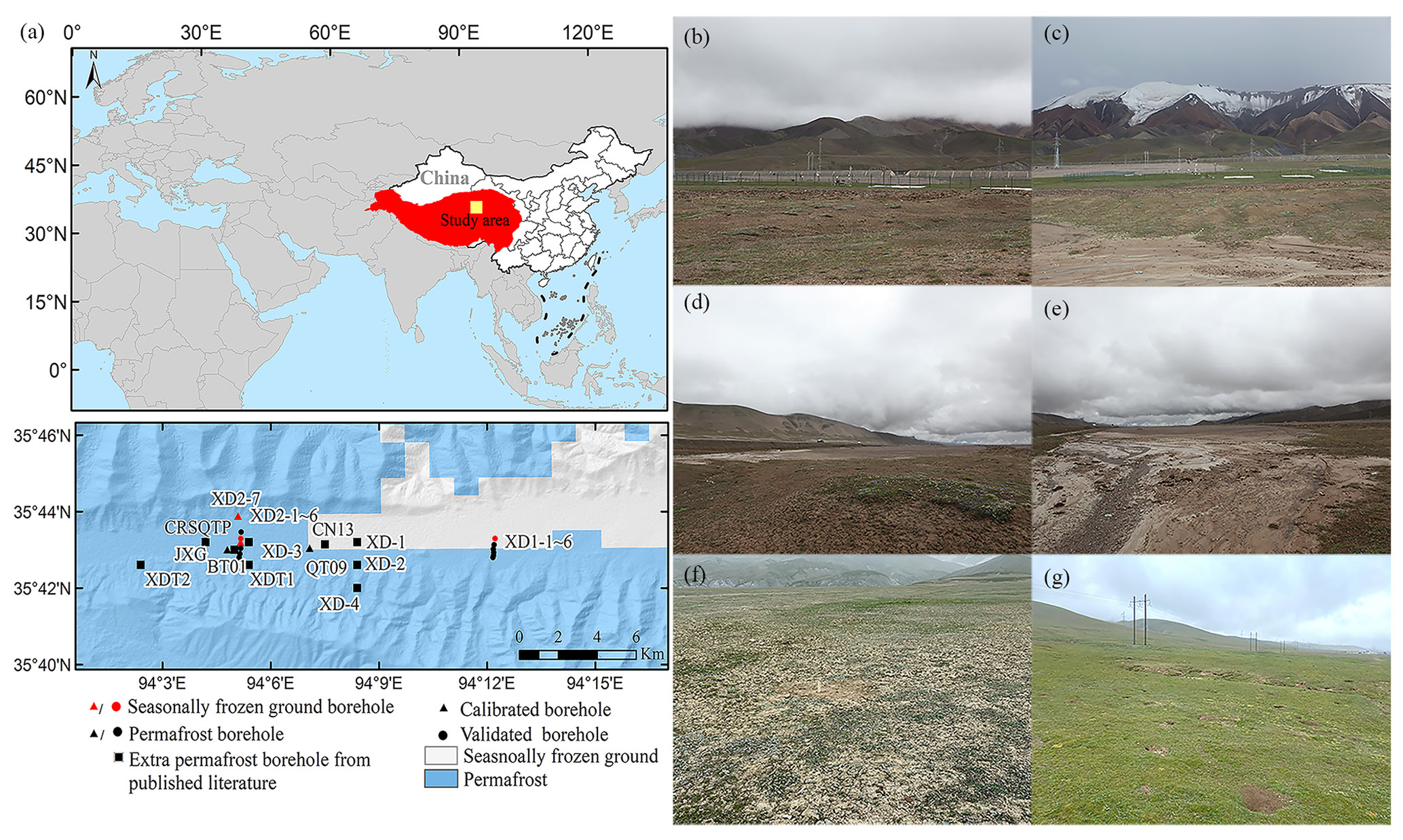
Figure 1 The geographical location of Xidatan on the QTP, its topography, and the location of 24 borehole sites (a). Surface conditions at monitoring borehole sites (b–g): view over the Xidatan COS (b); QT09, view towards the south (c); QT09, view towards the northeast (d); view from the vicinity of QT09 towards the east (e); XD2-1–XD2-7, view towards the south (f); XD1-1–XD1-6, view towards the east (g) (the spatial distribution of frozen ground types is derived from Zou et al., 2017; topography was generated by the digital elevation model (DEM) constructed from the Shuttle Radar Topography Mission (SRTM) with a 1 arcsec resolution (∼30 m); Jarvis et al., 2008; the Tibet Plateau boundary was taken from the National Tibetan Plateau Data Center; Zhang, 2019). All photographs were taken during the field investigation from 23 July to 2 August 2021.

2.2 Materials

2.2.1 Field monitoring and borehole observation datasets

There are 15 monitoring boreholes with long-term observations (for the last 10 years) established in Xidatan (Fig. 1a). A COS is in the central part of Xidatan, where the ground surface is composed of sparse dry alpine meadows and the soil layer is made of fluvial sand and gravel (Fig. 1b). A monitoring borehole QT09 (30 m deep at 4538 m a.s.l.) and an automatic weather station (AWS) automatically recorded long-term observed basic meteorological data, including the soil moisture content in the active layer (October 2009 to December 2018) and soil temperature at multiple depths (January 2005 to December 2017). Approximately 4 km from the COS, another 30 m deep borehole BT01 (4530 m a.s.l.) was drilled in sparse dry steppe with considerable coarse sand and gravel, where continuous soil temperature measurements were taken continuously at depths of 0.5 to 30 m spanning from 2004 to 2017. In these two sites, the soil moisture content in shallow layers (<1.1 m) ranged from 15 % to 39 % and from 4 % to 15 %, respectively, and the organic matter content was 4.2 % and 1.68 %, respectively (Liu et al., 2020).

In addition, during August 2012, 13 boreholes from 8 to 15 m depth (XD1-1–XD1-6, XD2-1–XD2-7) were drilled along parallel altitudinal transects in the east (3.15 km length) and west (3.86 km length) part of Xidatan (Luo et al., 2018). The soil temperature records are available at these borehole locations covering November 2012 to September 2017. Six boreholes (XD1-1–XD1-6) are located in dry and sparse grassland on the eastern altitudinal transect between 4368 and 4380 m a.s.l. (Fig. 1g); among these, the XD1-1–XD1-4 boreholes are all 15 m deep and the two other boreholes (XD1-5–XD1-6) are 8 m deep. A frozen layer has been observed in the five uppermost boreholes (XD1-1–XD1-5), while it was absent in the lowermost borehole XD1-6 (Luo et al., 2018). Similarly, seven boreholes were drilled at the western side of Xidatan, resulting in an altitudinal transect from 4490 m a.s.l. (in the north) down to 4507 m a.s.l. (in the south). The first three boreholes (XD2-1 to XD2-3) and XD2-6 are 15 m deep in sparse grassland. Similarly, boreholes XD2-4, XD2-5, and XD2-7, are 15, 15, and 8 m deep and located in river-erosion-induced sand-rich sediment (Fig. 1e). The ground temperature monitoring results showed that permafrost existed in boreholes XD2-1 to XD2-3 and XD2-6, but there was no permafrost in boreholes XD2-4 to XD2-5 and XD2-7 (Luo et al., 2018; Yin et al., 2021).

The air temperature (height of 2, 5, and 10 m) and the volumetric unfrozen soil water content in the active layer were recorded by a CR1000–CR3000 data acquisition instrument (Campbell Scientific, Logan, UT, USA, with ±0.5 ^∘C accuracy), and by a hydra-soil moisture sensor connected to a CR1000 data logger (Campbell Scientific, Logan, UT, USA, with an accuracy of ±2.5 %). A cable equipped with 20 to 30 high-accuracy (±0.1 ^∘C) thermistors (State Key Laboratory of Frozen Soil Engineering, Northwest Institute of Eco-Environment and Resources, Chinese Academy of Sciences – SKLFSE, NIEER, CAS) in a chain is connected to CR3000 and CR1000 (Campbell Scientific, Logan, UT, USA) data loggers and vertically arranged at depths from 0 to 30 m (the depths are not the same for all sites; details are given in Table A1). The ground temperature has been recorded automatically every 1 or 4 h at different depths. A more detailed description of the dataset, as well as of the thermistor setup and installations, can be found in Luo et al. (2018) and Zhao et al. (2021). Before proceeding further, errors in the sensor were identified and fixed, and the outliers were replaced with values generated by the data before and after (see Zhao et al., 2021, for more details on the quality control procedures). Then, the data were re-sampled for the daily average, used to calibrate and validate the model performance. The spatial distribution of these borehole sites is displayed in Fig. 1a, and the crucial information about these boreholes employed for model calibration and validation is summarized in Table A1.

2.2.2 Meteorological observations from the China Meteorological Administration

The observed temperature dataset from the China Meteorological Administration (CMA) ground-based meteorological stations was used to extend the land surface temperature (LST) series since the 1970s. For that, observed daily mean air temperature data for the 1970 to 2019 period at two AWSs of the CMA nearby (Wudaoliang: 35^∘13^′ N, 93^∘ 05^′ E; Golmud: 36^∘25^′ N, 94^∘55^′ E) were downloaded from the China Meteorological Data Service Center (http://data.cma.cn/, last access: 29 November 2022).

2.2.3 Remotely sensed land surface temperature datasets

A modified Moderate Resolution Imaging Spectroradiometer land surface temperature (MODIS LST) product is used to force a transient heat flow model for spatial modeling of alpine permafrost distribution. MODIS on board the Terra and Aqua satellites has provided LST measurements at a spatial resolution of 1 km×1 km since 2003 (https://modis.gsfc.nasa.gov/, last access: 29 November 2022). Here, we employ clear-sky MOD11A2 (Terra MODIS) and MYD11A2 (Aqua MODIS) products (processing version 6), which contain two observations (daytime and nighttime) per day for the same pixel (Zou et al., 2017). Before proceeding, time series of irregularly spaced observations owing to clouds or other factors were identified, and gaps were filled by the Harmonic ANalysis of Time Series (HANTS) algorithm (Obu et al., 2019). An empirical model (Zou et al., 2014, 2017) was subsequently established to obtain mean daily values from Aqua and Terra daytime and nighttime transient LST. Notably the model validation was quite good over Xidatan, with the square of the correlation coefficients (R²) above 0.9 (P<0.01). Details of these algorithms can be found in Xu et al. (2013) and Zou et al. (2014).

2.2.4 Additional validation datasets

Comprehensive investigation of permafrost and its environments in Xidatan in 1975 and 2012 was conducted (Nan et al., 2003; Luo et al., 2018). The lowest elevation of the permafrost boundary in 1975 and 2012 was approximately 4360 and 4388 m a.s.l., respectively, by ground-penetrating radar (GPR) profiles combined with drilling boreholes. Subsequently, permafrost distribution in this region was delineated on a topographic map at a scale of 1:50 000 by hand empirically using contour elevation line based on the field survey data, aerial photographs, and satellite images (Fig. 2a–b). In addition, one benchmark map of permafrost distribution in 2016 was created by Zou et al. (2017), simulated by the temperature at the top of the permafrost (TTOP) model (Fig. 2c). The abovementioned three maps were used as the validation data to evaluate model performance in permafrost distribution. Furthermore, the long-term continuous ALT observation dataset for BT01, QT09, XD1, XD2-4, and XD2-6 interpolated from the in situ soil temperature profile (Liu et al., 2020; Yin et al., 2021) was also used to evaluate the model performance. Moreover, the observed permafrost distribution of boreholes (CRSQTP, JXG, XD1, XD2, XD3, XD4, XDT1, XDT2, CN13) was used to assist in determining whether permafrost existed or not.

2.3 Methods

2.3.1 Model description

We simulated the subsurface temperature dynamics along the soil column by numerically solving the one-dimensional transient Fourier's law heat conduction equation. The model physical basis and operational details are documented in Sun et al. (2019), and only a brief overview of the model properties for a single grid cell is given here. Ground temperature T changes over time t and depth Z through heat conduction, as described by

$$\begin{array}{}\text{(1)}& C_{\mathrm{eff}}\left(z,T\right){\displaystyle \frac{\partial T}{\partial t}}-k\left(z,T\right){\displaystyle \frac{\partial }{\partial z}}\left({\displaystyle \frac{\partial T}{\partial z}}\right)=\mathrm{0},\end{array}$$

with a constant geothermal heat flow of Q_geo=0.08 W m⁻² as the lower boundary condition (Wu et al., 2010) and LST as the upper boundary condition. The thermal properties of the ground are described in terms of heat capacity C, thermal conductivity k, and total volumetric water/ice content VWC. The latent heat effects of the water–ice phase transition is accounted for in terms of an effective heat capacity C_eff (z, T). The heat transfer equation (Eq. 1) was discretized along with a soil domain to 100 m depth using finite differences. Subsequently, the trapezoidal rule was applied to numerically solve moderately stiff ordinary differential equations (Schiesser, 1991; Westermann et al., 2013). With comprehensive consideration of the modeling precision and computation cost, we choose the calculated time step to be 1 d and set a total of 282 vertical levels for each soil column, with the vertical-resolution configurations of 0.05 m (the upper 4 m) and 0.5 m (remaining soil layer to 100 m).

2.3.2 Model calibration and validation

We selected four borehole sets (Fig. 1a), which represented different soil type classes with various thermal properties, for the initial model calibration and the remaining sites for cross-validation. The sites were selected based on surface deposits, vegetation coverage, and soil types at a 1 km×1 km spatial resolution (Li et al., 2015b; Luo et al., 2018). Thermophysical properties (e.g., stratigraphies, texture, ground ice content, organic matter content, dry bulk density) of distinct soil layers were measured or assessed from field surveys, laboratory measurements, and on-site measurements of soil samples obtained from 15 borehole cores (depths between 8–30 m). These boreholes were specific to each soil class and geographical location. For detailed information for the bulk density and moisture content measurements of soil samples, refer to Zhao and Sheng (2015). Furthermore, a time series of an observed soil water content dataset in the active layer (Sun et al., 2019, 2022; Zhao et al., 2021) vicinity of the site (QT09) and the ground ice distribution maps created by Zhao et al. (2010a) are used for water content estimates of each soil type. And then, we pre-selected narrow ranges of plausible values of typical soil thermophysical parameters (thermal conductivity and heat capacity; for details see Table A2); and finely adjusted them during model calibration. The manual stepwise optimization procedures were used to adjust parameters based on the suggestions by Hipp et al. (2012). Specifically, calibration was performed by systematically changing k over the given plausible ranges to improve the agreement between the simulated and observed ground temperature at different depth levels. Subsequently, minor adjustments were made to C to promote the model's performance.

The model was initialized by cyclical forcing of the first-year LST data until the soil temperature profile reached a steady state to estimate an initial temperature profile. The number of spin-up cycles was between 2000 and 3300, and the criterion of the soil temperature profile reaching equilibrium under the upper and lower boundary condition was set at less than 0.0001 ^∘C per cycle. The last-day ground temperature profile was subsequently used as the initial condition for subsequent modeling. The agreement between the model grid and borehole monitoring site was quantified at each depth in terms of the mean absolute error (MAE) and root mean square error (RMSE) (Willmott and Matsuura, 2005; Jafarov et al., 2012):

$$\begin{array}{}\text{(2)}& {\displaystyle }\mathrm{MAE}={\displaystyle \frac{\mathrm{1}}{n}}\sum _{i=\mathrm{1}}^n\mathrm{|}{\mathrm{Ob}}_i-{\mathrm{Sm}}_i\mathrm{|},\text{(3)}& {\displaystyle }\mathrm{RMSE}=\sqrt{{\displaystyle \frac{{\sum }_{i=\mathrm{1}}^n({\mathrm{Ob}}_i-{\mathrm{Sm}}_i{)}^{\mathrm{2}}}{n}}},\end{array}$$

where Ob_i, Sm_i is the observation and simulation value, respectively. And n is the total number of data. The MAE shows an overall error between observing and simulating when the RMSE emphasizes an error variation.

2.3.3 Historical and future long-term LST series

We extended LST by establishing statistical relationships between local LST and air temperature (AT) from nearby AWSs to derive historical and future LST series for each grid from historical (1970–2019) AT observation and the multi-model ensemble AT projection by 2100 under different climate change scenarios.

The AT_cma, AT, and LST denote the air temperature from the CMA, air temperature at 2 m from our COS, and ground surface temperature derived from modified MODIS LST, respectively. Firstly, we established a linear regression between LST and AT from the measured period of 2004 to 2018, where the temperature variability was highly correlated between LST and AT with R²=0.83 and P<0.01; secondly, the daily AT series from 1970 to 2019 were generated utilizing a stepwise linear regression between measured AT from 2004 to 2018 and those values extracted from CMA meteorological stations (AT_cma) nearby, which worked well with R²=0.88 and P<0.01; thirdly, we generated a time series of LST staring from 1970 based on the AT–LST linear regression model induced in step 1 and extending the AT series in step 2.

For future AT projections, the Sixth Assessment Report of the Intergovernmental Panel on Climate Change Working Group I (IPCC WG 1 AR6) (Iturbide et al., 2020; IPCC, 2021) has evaluated and projected climate change over the QTP during the 21st century (https://interactive-atlas.ipcc.ch, last access: 29 November 2022). The model estimated warming between 1995–2014 and 2081–2100 of the mean annual AT in the QTP under three RCPs scenarios as 0.013 ^∘C a⁻¹ (RCP2.6, low concentration of emissions), 0.028 ^∘C a⁻¹ (RCP4.5, stable concentration of emissions), and 0.060 ^∘C a⁻¹ (RCP8.5, high concentration of emission) calculated from the multi-model ensemble median (21–29 model outputs) of CMIP5. The mean warming rate is 0.017 ^∘C a⁻¹ (SSP1-2.6, strong climate change mitigation), 0.032 ^∘C a⁻¹ (SSP2-4.5, moderate mitigation), and 0.064 ^∘C a⁻¹ (SSP5-8.5, no mitigation), estimated from the CMIP6 ensemble median of 31–34 model outputs. Using the AT–LST linear regression relationship model, we obtained a mean LST warming rate of 0.012 (RCP2.6), 0.025 (RCP4.5), and 0.050 ^∘C a⁻¹ (RCP8), and a mean LST increase rate of 0.015 (SSP1-2.6), 0.030 (SSP4-4.5), and 0.057 ^∘C a⁻¹(SSP5-8.5).

2.3.4 Spatial modeling

The extended and projected LSTs were used to force our calibrated model for simulating the spatial distribution of permafrost in Xidatan. The ground thermal regime was simulated for a specific ground stratigraphy under boundary conditions from a one-dimensional multilayer soil profile down to 100 m depth at each grid point. The thermophysical parameters of multilayer soil columns were specified and assigned for each soil type based on the soil type map at 1 km×1 km spatial resolution (Li et al., 2015b). If the maximum temperature of any soil layer in the grid point was ≤0 ^∘C for 2 consecutive years, the model cells were identified as permafrost. In contrast, the seasonally frozen ground was defined from the not-yet-assigned cells, in which the minimum soil temperature of any layer in the same 2 years was ≤0 ^∘C. The remaining cells were unfrozen ground (Wu et al., 2018). The continuous permafrost zone was defined as the region where the area coverage of permafrost is more than 90 % (of the total area). Otherwise, it was demarcated as a discontinuous permafrost zone (Qin, 2014). The simulation domain comprises about 280 km² with a horizontal resolution of 1 km×1 km, corresponding to 280 independent runs.

3 Result

3.1 Model evaluation

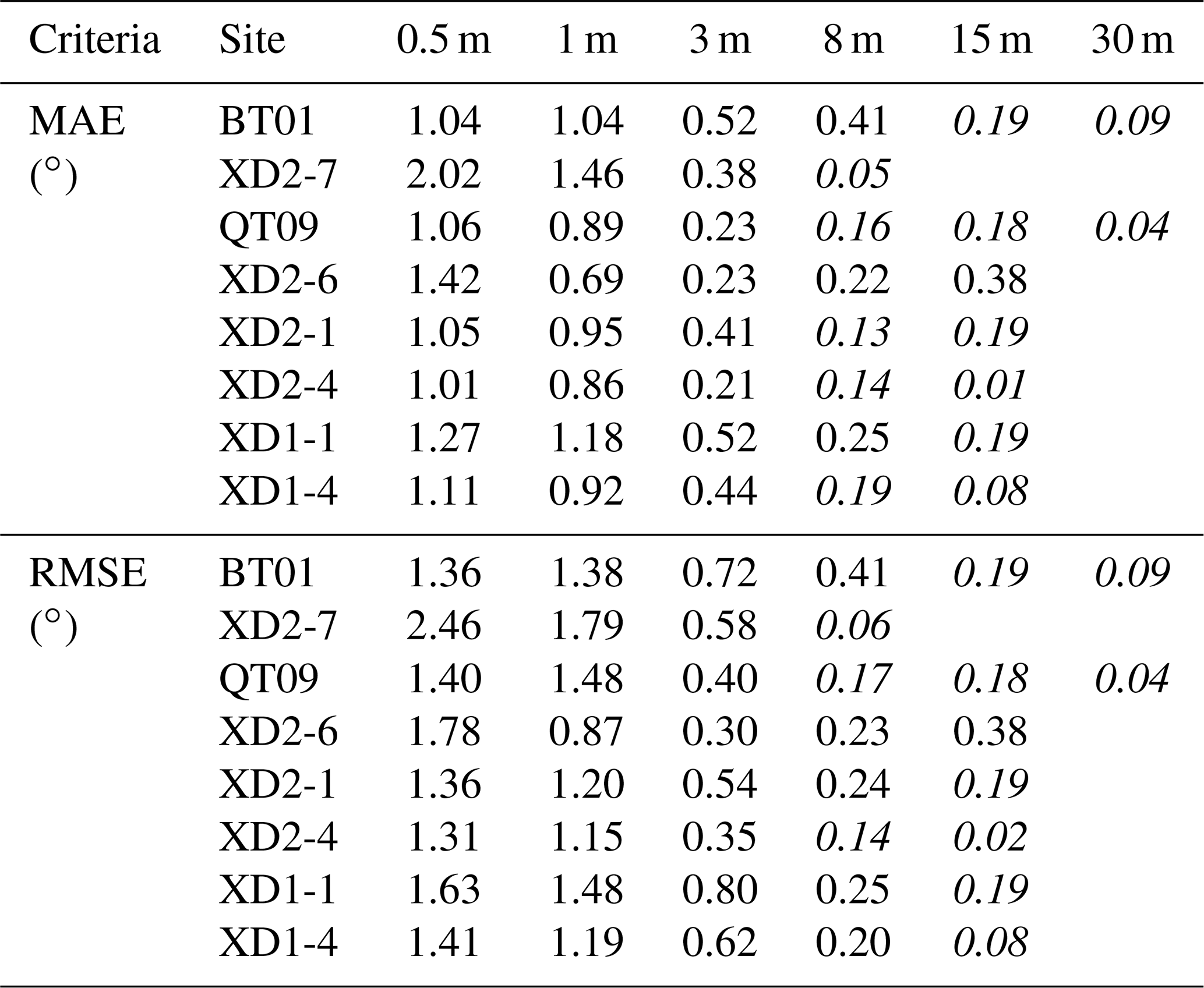
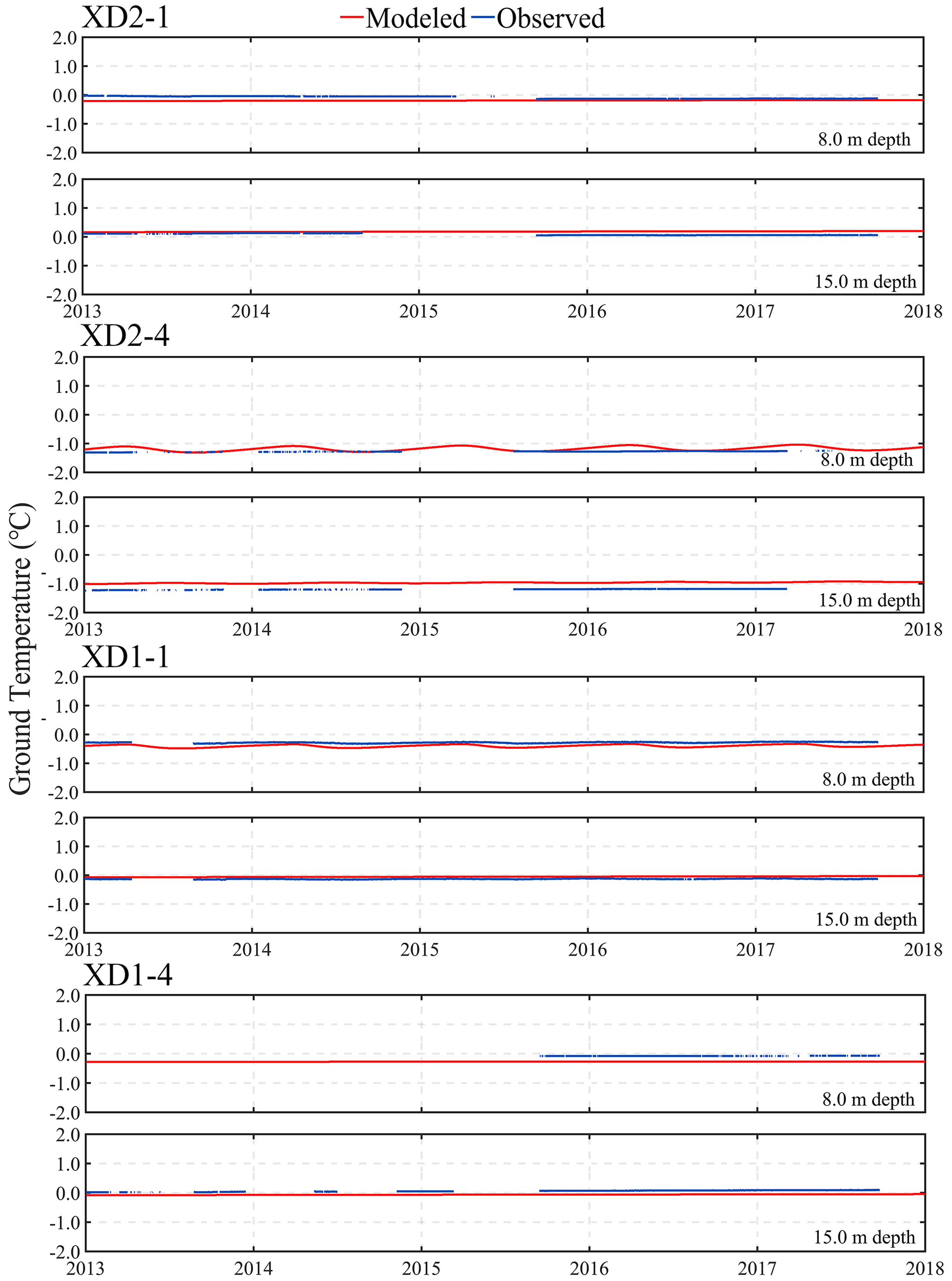
Simulated ground temperature results demonstrate relatively large bias (with the MAE ranging from 0.69 to 2.02 ^∘C and RMSE ranging from 0.87 to 2.46 ^∘C) for the surface soil layer to 1 m in depth at all calibration sites (Table 1 and Fig. A1). This could be explained by the frequent fluctuation in and complex variation pattern of ground temperature itself at shallow depth being greatly affected by local factors (e.g., terrain, waterbodies, snow cover, vegetation). However, these discrepancies between simulated and observed ground temperature gradually reduce with the increase in soil depth. Most calibration boreholes showed a good correspondence between modeled and measured ground temperature at the intermediate (3, 8 m) and deep (15, 30 m) layers (Fig. A2), with an MAE of 0.05–0.52 ^∘C and 0.04–0.38 ^∘C, as well as an RMSE of 0.06–0.58 ^∘C and 0.04–0.38 ^∘C, respectively (Table 1). The same pattern appeared at validation sites (Figs. A3–A4). Ground temperatures in validation sites were equally well reproduced by the calibrated model, yielding an MAE of 0.86–1.27 ^∘C (RMSE of 1.15–1.63 ^∘C) in the 0.5 and 1 m layers and 0.01–0.52 ^∘C (RMSE of 0.08–0.80 ^∘C) in the 3 and 15 m layers (Table 1). Generally, the consistent daily fluctuations in the simulated and observed soil temperature at all observational depths for most calibration and validation sites indicated the satisfactory simulation by our calibrated model.

Site XD2-6 has relatively poor performance in the deep layer (8 and 15 m) compared with the shallow layers (Fig. A2). The deviation between measured and simulated soil temperature in this special case might be caused by micro-scale heterogeneity in surface cover, topography, and soil stratigraphy at the sub-grid scale, which led to more difficulty in accurate modeling. Nevertheless, the deviation between these modeled results and measured values is within 0.38 ^∘C at the deep layer (15 m). Furthermore, the permafrost at this site was simulated to disappear in the middle to late 2010s, which was in line with the observation (Yin et al., 2021).

Table 1 Error metrics for assessing daily average ground temperature at different depths derived from observation and simulated for individual calibration and validation sites (good criteria values <0.20 ^∘C are displayed in italics).

To better estimate the model performance in spatial modeling, we compared our simulations with three permafrost maps based on 1975, 2012, and 2016. Based on the validation of the various maps against the permafrost and seasonally frozen ground observation at 24 boreholes (Fig. 2), we found that both the 1975 and the 2012 maps can well interpret the continuous permafrost zone at central-western Xidatan. However, there are many erroneous (12.5 % for 1975 and 16.6 % for 2012) recognitions of seasonally frozen ground in the discontinuous permafrost zone. This indicated that these two permafrost maps could not well represent the historical permafrost distribution status in the study region permafrost and seasonally frozen ground coexisting zones. In addition, these two maps are strongly inconsistent with the 2016 map and our simulations (Fig. 2a–b). The 2016 map and our simulations showed a consistent permafrost distribution pattern and correctly identified almost all continuous permafrost locations (Fig. 2c–f). However, a slight discrepancy existed between the 2016 map and our simulation in permafrost (8.3 %) and seasonally frozen ground (8.3 %) locations over the margins of the discontinuous–continuous permafrost zone. Our simulated results were consistent with the investigated results and indicated good recognition of the seasonally frozen ground in this region.

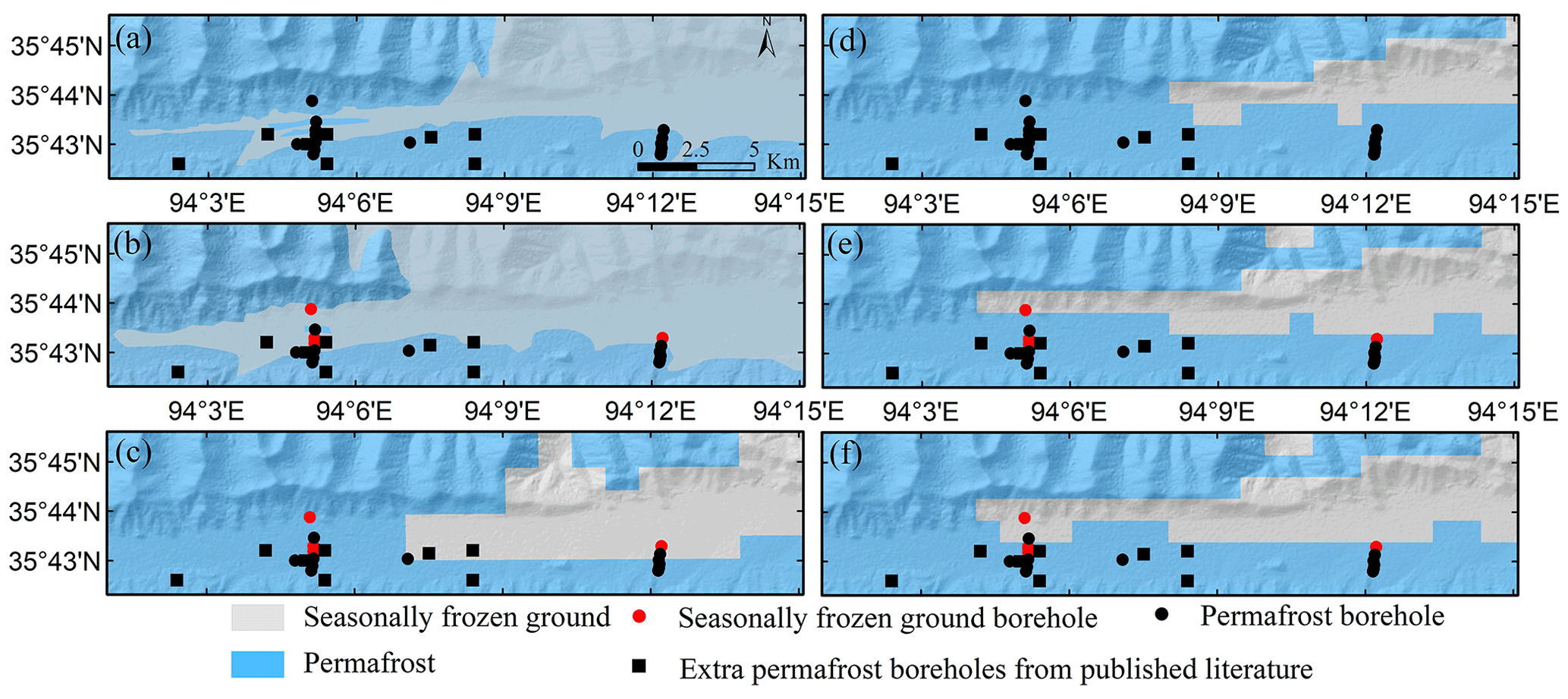
Figure 2 Geographic distribution of permafrost and seasonally frozen ground across Xidatan for three permafrost maps in 1975, 2012, and 2016 (left panels: 1975 a, 2012, b, 2016 c, published in Nan et al., 2003; Luo et al., 2018; Zou et al., 2017) compared to corresponding modeled outputs (right panels: 1975 d, 2012 e, 2016 f).

Continuous multi-year ALTs derived from five monitoring sites were compared with those from the model-simulated (Fig. 3). The results indicated that there is a strong positive correlation between the simulated and observed ALT (R²=0.98, P<0.01), and the simulation bias in the ALT from these sites is within ±0.25 m. In terms of geographical structure, the spatial characteristics of ALT across the study area are well captured by our model. Both observed and simulated ALT in XD2-6 varied from 4.15 to 4.31 m, which is higher than at other sites (BT01: 2.55 to 2.85 m; QT09: 1.45 to 1.60 m; XD2-1: 2.30 to 2.48 m; XD2-3: 2.95 to 3.05 m).

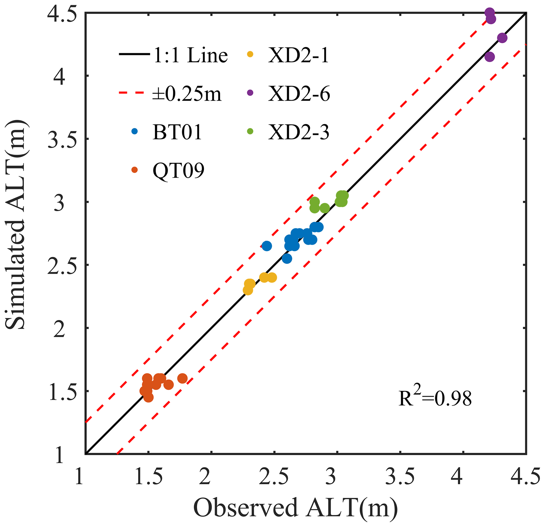
Figure 3 Comparison between annually observed ALT and that simulated at different sites (for TB01 and QT09 – Liu et al., 2020; Zhao et al., 2021 – observations from 2005 to 2017 and 2005 to 2018, respectively, are available; observation periods at XD2-1, XD2-3, and XD2-6 – Yin et al., 2021 – are from 2013 to 2019 and 2013 to 2017). The solid line is a 1:1 line, and the dashed line shows biases within ±0.25 m; dots are colored to represent the different sites.

3.2 Historical permafrost evolution

Our simulation outputs were combined with topographic data (elevation and slopes) derived from a 30 m DEM to analyze the permafrost distribution and its dynamics. The MAGT at the depths of ZAA, permafrost table, permafrost base, and permafrost thickness are defined from vertical temperature profiles as critical parameters to describe the permafrost thermal regime, which was also chosen for analysis and discussion. Areas with seasonally frozen ground were excluded from the subsequent studies.

3.2.1 Initial situation of permafrost distribution

The simulation results (Table 2, Fig. 4) showed the initial situation in 1970. The lower limit of modeled continuous permafrost was ca. 4525 and 4732 m a.s.l. on the north- and south-facing slopes, respectively, while the lowest elevation of the permafrost boundary simulation was 4138 m a.s.l. (on the north-facing slopes) and 4357 m a.s.l. (on the south-facing slopes). Approximately 80 % of the total counting area was underlain by permafrost (33.93 % was continuous, and 46.07 % was discontinuous) in Xidatan. Regionally, the distribution characteristics of permafrost conditions are predominantly controlled by elevations. With altitude ascending westwards gradually, the permafrost temperature and permafrost table show a decreasing trend, whereas the position of the permafrost base and permafrost thickness increase. Furthermore, local topographic factors in slope also govern permafrost distribution in the study area. Permafrost temperature on the north-facing slopes was far colder than that on the south-facing slopes within the same elevations (Fig. 4a). On the south-facing slopes (with high altitudes above 4500 m a.s.l.) and north-facing slopes modeled results show a comparatively cold permafrost temperature (MAGT ranges from −0.5 to −4.5 ^∘C). The simulated permafrost table was less than 2.5 m, with a permafrost base of 20 to 48 m and permafrost of up to 46 m at the maximum extent, whereas on the south-facing slopes with low altitudes below 4500 m a.s.l., modeled MAGT is higher than −0.5 ^∘C, the position of the modeled permafrost table varies from 2.5 to 4.5 m, the permafrost base is at a depth of fewer than 20 m, and permafrost thickness is approximately 4 m at the thinnest point.

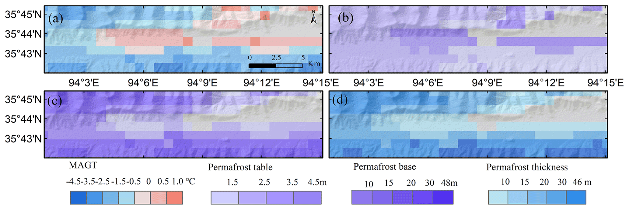
Figure 4 Spatial distributive features of the MAGT (a), permafrost table (b), permafrost base (c), and permafrost thickness (d) for the initial simulation of the 1970s over Xidatan (grey areas with the seasonally frozen ground were excluded).

3.2.2 Changes in permafrost conditions

From 1970 to 2019, the simulation results indicate that the lower limit of the continuous permafrost zone remained unchanged over the study areas. The lowest elevation of the permafrost boundary had a remarkable rise of 47 m on the north-facing slopes, while that remained unchanged on the south-facing slopes. Correspondingly, around 12.86 % of the discontinuous permafrost zone transformed into seasonally frozen ground (Table 2), which caused the northern boundary of the discontinuous permafrost zone to retreated approximately southwards by 1–2 km, but the continuous permafrost zone was unchanged (Fig. 5).

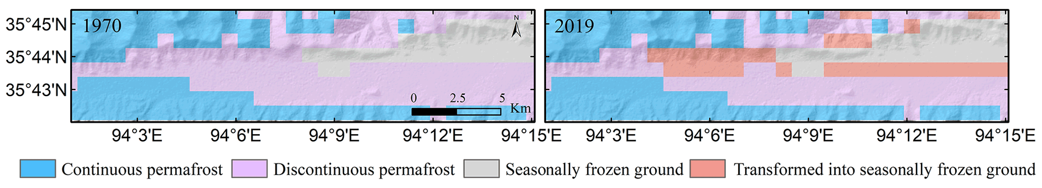
Figure 5 Spatial distributive changes in the continuous and discontinuous permafrost and seasonally frozen ground zone over Xidatan from 1970 to 2019.

Table 2 Variations in the permafrost boundary and areal extent of the frozen ground type over Xidatan for 1970–2019 and projected variations by 2100 under different climate change scenarios.

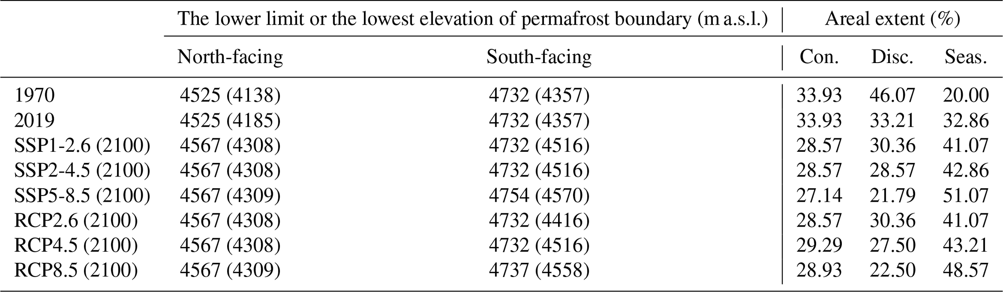
Note: outside parentheses is the lower limit of the permafrost, while inside parentheses is the lowest elevation of the permafrost boundary. Con., Disc., and Seas. indicate continuous permafrost, discontinuous permafrost, and seasonally frozen ground.

The regional-average MAGT has increased by 0.44 ^∘C over the past 50 years. With temperature warming, we found a gradual decline with a mean amplitude of 0.36 m in the position of the permafrost table, whereas there was a drastically raised permafrost base by 1.12 m. Correspondingly, permafrost had thawed with an average of nearly 1.54 m in thickness. Spatially, the mean MAGT warmed up to 0.49 ^∘C, and the average permafrost table declined by 0.37 m for the continuous permafrost zone, but its permafrost base (around −0.80 m) and thickness (around −1.18 m) variations were comparatively slight. By comparison, relatively low variations in MAGT (0.40 ^∘C) and in the permafrost table (average decline by 0.76 m) but dramatic changes with a mean decline of −4.23 m occurred in the discontinuous permafrost zone, which is roughly twice that of changes in the continuous permafrost area. Correspondingly, an average of about −1.96 m in thick permafrost quickly thawed, owing to a remarkable rising effect of the permafrost base.

Table 3 Changes in characteristics of the frozen ground type over Xidatan for 1970 to 2019 and projected changes by the 2090s, relative to the 2010s, under different climate change scenarios.

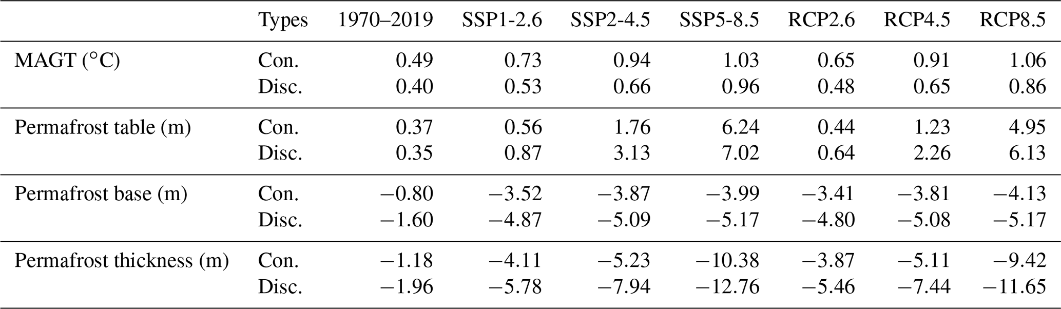
Note: Con., Disc., and Seas. indicate continuous permafrost, discontinuous permafrost, and seasonally frozen ground.

3.3 Projection of permafrost conditions

The projected changes in the lower limit of permafrost, the lowest elevation of the permafrost boundary, and the spatial distribution of continuous and discontinuous permafrost and seasonally frozen ground as well as their characteristics (MAGT, permafrost table, permafrost base, and permafrost thickness) are presented in Tables 2–3 and Fig. 6.

The result indicates that the lower limit of permafrost on the north-facing slopes is projected to increase by 42 m until 2100, relative to 2019, under all RCPs or SSPs. On the south-facing slopes, this value is about 22 m under very high emission scenarios (SSP5-8.5 or RCP8.5), which is far smaller than the changes in the lowest elevation of the permafrost boundary. The lowest elevation of the permafrost boundary on the north-facing slopes is projected to increase by 123 m by 2100, relative to 2019, under both low- and medium-emission scenarios, and by 124 m under very high emission scenarios SSP5-8.5 or RCP8.5. South-facing slopes are projected to increase by 159 m by 2100, compared to 2019, under both low and medium emissions of RCP or SSP scenarios. Still, a more pronounced increase of around 213 and 201 m is projected under SSP5-8.5 and RCP8.5. Relative to 2019, the areal extent of continuous permafrost zone is projected to decrease by 5.36 (5.36), 5.36 (4.64), and 6.79 (5.00) % by 2100 under SSP1-2.6 (RCP2.6), SSP2-4.5 (RCP4.5), and SSP5-8.5 (RCP8.5), respectively, compared with a decrease of 3.57 (2.85), 4.64 (5.71), and 11.42 (10.71) % for the discontinuous permafrost zone. In contrast, the areal extent of seasonally frozen ground is projected to increase by 8.93 (8.21), 10.00 (10.36), and 18.21 (15.71) % by 2100, relative to 2019, under SSP1-2.6 (RCP2.6), SSP2-4.5 (RCP4.5), and SSP5-8.5 (RCP8.5), respectively. The northern limit of the continuous permafrost zone is projected to retreat southwards by around 1–2 km under SSP1-2.6 (RCP2.6), SSP2-4.5 (RCP4.5), or RCP8.5 and by about 1–3 km under SSP5-8.5. By comparison, the northern boundary of the discontinuous permafrost zone is anticipated to shift southwards by around 1 km under SSP1-2.6 (RCP2.6) or SSP2-4.5 (RCP4.5) and by around 1–2 km under SSP5-8.5 (RCP8.5).

Figure 6 Projected spatial distributive changes in frozen ground type over Xidatan by 2100 under RCP and SSP scenarios (left column, under a SSP1-2.6, c SSP2-4.5, and e SSP5-8.5 scenarios; right column, under b RCP2.6, d RCP4.5, and f RCP8.5 scenarios).

Under global climate warming scenarios, the permafrost temperature is anticipated to increase further, but its variation lags substantially behind the changes in air temperature. Relative to the 2010s, the regional-average MAGT is projected to warm by 0.63, 0.81, and 0.99 ^∘C by the 2090s under SSP1-2.6, SSP2-4.5, SSP5-8.5, respectively, which is slightly higher than that of RCP scenarios (0.56, 0.78, and 0.98 ^∘C, respectively). Along with MAGT rising, relative to the 2010s, the permafrost table is projected to further decline by 0.72 to 6.70 m under SSP scenarios (0.72, 2.48, and 6.70 m under SSP1-2.6, SSP2-4.5, and SSP5-8.5, respectively) and decline by 0.54 to 5.47 m under RCP scenarios (0.54, 1.73, and 5.47 m under RCP2.6, RCP4.5, and RCP8.5, respectively), at the end of the century (the 2090s). The average permafrost base is projected to rise by 4.22, 4.54, and 4.56 m by the 2090s, compared to the 2010s, under SSP1-2.6, SSP2-4.5, and SSP5-8.5, respectively. Meanwhile, a relative decrease in the permafrost base of 4.14, 4.43, and 4.60 m is estimated under RCP2.6, RCP4.5, and RCP8.5, respectively. An average thinning in the permafrost thickness is projected to be 4.97, 6.66, and 11.74 m under SSP1-2.6, SSP2-4.5, and SSP5-8.5, respectively, and that would be 4.71, 6.26, and 10.43 m under RCP2.6, RCP4.5, and RCP8.5, respectively.

Spatially, the average MAGT is projected to rise by 0.73 (0.65), 0.94 (0.91), and 1.03 (1.06) ^∘C for the continuous permafrost zone under SSP1-2.6 (RCP2.6), SSP2-4.5 (RCP4.5), and SSP5-8.5 (RCP8.5), respectively, compared with a rise of 0.53 (0.48), 0.66 (0.65), and 0.96 (0.86) ^∘C, respectively, for the discontinuous permafrost zone. As for the permafrost table, both the continuous and the discontinuous permafrost zone is projected to gradually decline under SSP1-2.6 (0.56 and 0.87 m) and RCP2.6 (0.44 and 0.64 m), but a remarkable decline is projected under medium-emission and very high emission scenarios, and a more pronounced decline is anticipated under SSPs scenarios than indicated by projection under RCP scenarios. The average permafrost table in the continuous permafrost zone is projected to decline by 1.76 (1.23) and 6.24 (4.95) m under SSP2-4.5 (RCP4.5) and SSP5-8.5 (RCP8.5), respectively, compared with a decline of 3.13 (2.26) and 7.02 (6.13) m under SSP2-4.5 (RCP4.5) and SSP5-8.5 (RCP8.5), respectively, for the continuous permafrost zone. The permafrost base is projected to rise remarkably under all scenarios. For the continuous permafrost zone, the permafrost base is projected to rise by 3.52 (3.41), 3.87 (3.81), and 4.13 (3.99) m under SSP1-2.6 (RCP2.6), SSP2-4.5 (RCP4.5), and SSP5-8.5 (RCP8.5), respectively, which is slightly smaller than that projected for the discontinuous permafrost zone (4.87 (4.80), 5.09 (5.08), and 5.17 (5.17) m under SSP1-2.6 (RCP2.6), SSP2-4.5 (RCP4.5), and SSP5-8.5 (RCP8.5), respectively). The average permafrost thickness of the continuous and discontinuous permafrost zone is projected to thin 4.11 (3.87) and 5.78 (5.46) m, respectively, under SSP1-2.6 (RCP2.6) as the main effect of the permafrost base rising, whereas there is a more prominent decrease of 5.23 (5.11) and 7.94 (7.44) m, respectively, under SSP2-4.5 (RCP4.5) and of 10.38 (12.76) and 9.42 (11.65) m, respectively, under SSP5-8.5 (RCP8.5) owing to the effect of both the permafrost table declining and the permafrost base rising.

4 Discussion

4.1 Comparison with previous studies

In this work, our simulated distribution of the continuous permafrost zone had substantial agreement with three permafrost maps based on 1975, 2012, and 2016. Still, there was a remarkable difference in the discontinuous permafrost zone where permafrost and seasonally frozen ground coexist (Fig. 2). Compared with the 2016 map and our simulated results, the 1975 and 2012 maps underestimated the permafrost area in the discontinuous permafrost zone. This contradiction might be due to differences using data, methods, study periods, spatial resolutions, etc. (Yang et al., 2010; Ran et al., 2012; Zou et al., 2017). The 1975 and 2012 maps were plotted on a topographic map at a 1:50 000 scale based on field investigations, aerial photographs, and satellite images (Nan et al., 2003; Luo et al., 2018). These coarse-resolution maps cannot accurately consider the effect of local factors, since they cannot describe variations in ground conditions over a short distance (Zhang et al., 2013). Moreover, comparing them with field observations makes the results difficult to validate. Although the 1975 and 2012 maps may represent the corresponding permafrost status in that year, they are limited by field investigations, and there is not a clear understanding of whether permafrost existed in the northeastern high-altitude areas or not. In the 2012 map, these isolated upper mountain areas are uniformly considered the seasonally frozen ground when mapping permafrost (Luo et al., 2018), which is unreasonable and underestimates the areal coverage of the permafrost in that area. Furthermore, the artifactual errors were hard to control when mapping permafrost distribution by conventional cartographic techniques that manually delineated the permafrost boundaries on the topographic maps (Zou et al., 2017; Ran et al., 2012). These factors inevitably led to uncertainties existing in the 1975 and 2012 maps.

By comparison, the 2016 map and our simulation results have a much higher spatial resolution (1 km×1 km) than field-investigation-based ones (e.g., 1975 and 2012 maps) by improved MODIS LST application. In addition, they showed higher accuracy in identifying both permafrost and seasonally frozen ground boreholes and performed better at recognizing the seasonally frozen ground in regions with complex terrain. This finding highlights the potential advantage of remote-sensing-based data in improving the spatial modeling of marginal permafrost simulations on the QTP. Overall, our simulated distribution of continuous permafrost and discontinuous permafrost zones was similar to that of the 2016 map. Differences mainly due to the TTOP model did not consider the thermal state of the deep permafrost. Therefore, the areal extent of permafrost distribution in the 2016 map was likely slightly underestimated compared with our simulation results. Moreover, the 2016 map assumes that permafrost is in equilibrium with the long-term climate. However, the ground temperature observations of permafrost on the QTP have increased during the past several decades (Zou et al., 2017; Zhao et al., 2010b, 2020; Yao et al., 2019; Ehlers et al., 2022), and this means a disequilibrium of permafrost under ongoing global warming. So, a map based on a contemporary climate forcing will likely underestimate the permafrost extent (Zou et al., 2017). By contrast, in our study, we used a transient numerical heat conduction permafrost model, which integrated climate and ground condition variables to quantify the change in permafrost. Our model performed well in modeling the evolution and disappearance of two permafrost islands after 1975 and the shifting northern boundary of discontinuous permafrost (Fig. 2d–f), which can be confirmed by direct observation (Jin et al., 2006; Luo et al., 2018; Yin et al., 2021). These phenomena implied our model could accurately capture marginal permafrost thermal state dynamics under a warming climate.

Furthermore, using our model, we quantified the spatial distribution of permafrost over the study area. We simulated a striking elevation dependence in permafrost distribution. Specifically, permafrost temperature decreases, permafrost decreases in thickness, and the permafrost table becomes thinner with the increased elevation, which is consistent with previous observation-based studies (Cheng et al., 1984; Wu et al., 2010; Zhao et al., 2010b, 2019, 2020; Li et al., 2012; Jin et al., 2011; Luo et al., 2018). Moreover, Cheng et al. (2019) further indicated that the MAGT varied from −5 to 0.5 ^∘C and the average permafrost thickness was approximately 26 m, as deduced by a considerable monitoring and field investigation dataset. The monitoring network of ALT along the Qinghai–Tibet Highway (QTH) (Li et al., 2012) has demonstrated that the mean ALT was 218 cm, ranging from 100 to 320 cm from 1981 to 2010. This evidence strongly corroborates our simulation result accuracy, giving us more confidence in upscaling our model to the study area to investigate spatiotemporal dynamics and anticipate possible changes in permafrost.

4.2 Process of permafrost degradation

In this paper, we simulated a slow response of the permafrost thermal state to a warming climate in the northern lower limit of the permafrost zone (Xidatan) on the QTP. As shown in our simulation, from 1970 to 2019, we simulated that roughly 12.86 % of the discontinuous permafrost zone over the study area has ultimately converted into seasonally frozen ground, which is very close to observed data (13.8 %) here in 2012 (Luo et al., 2018). Permafrost distribution and its thermal conditions over the study area were spatially controlled by elevation. In addition, the orientation of the slope influenced the amount of solar radiation received by the ground surface (Cheng, 2004), specifically causing much thicker, colder permafrost and a thinner ALT on the north-facing slopes than on the south-facing slopes within the same elevation. So, there was a distinct spatial discrepancy of permafrost thermal regimes in response to a warming climate in different thermal states. Over the past 50 years, the rising rate of MAGT for the continuous permafrost zone has been relatively fast (regional average warmed by 0.49 ^∘C) due to more energy being available to heat the ground. By contrast, as permafrost temperature has moved close to the thawing point (about 0 ^∘C), accumulated energy has been enormously consumed by melting ground ice, and MAGT for the discontinuous permafrost zone has slowly risen (regional average warmed by 0.40 ^∘C). Meanwhile, both the continuous (regional average declined by 0.37 m) and discontinuous permafrost zone (regional average declined by 0.35 m) displayed a gradual decline in the position of the permafrost table. But we simulated a drastically risen permafrost base, especially in the discontinuous permafrost zone, due to heat transfer in strata from the top to bottom, leading the geothermal gradients in permafrost to keep dropping. When the geothermal gradient in permafrost temperature drops to less than that of the underlying thawed soil layers, the geothermal heat flux from the deep stratum is completely used to thaw the permafrost base. Hence, permafrost thaws from bottom to top and moves upwards. As permafrost is relatively warm and thin and geothermal flow relatively high over Xidatan (Wu et al., 2010; Sun et al., 2019), the main degradation mode of permafrost over this region is simulated to be upward thawing from the permafrost base. This degradation mode is also confirmed by several monitoring boreholes across this region (Jin et al., 2006, 2011; Cheng and Wu, 2007; Liu et al., 2020). In general, the pattern of permafrost degradation over Xidatan from 1970 to 2019 can be summarized as the continuous permafrost zone being gradually converted to warm permafrost, whereas the discontinuous permafrost zone has been thawing upwards remarkably. Notably, the margin of the discontinuous permafrost zone has converted to seasonally frozen ground.

As for the projections under different climate change scenarios, the latest generation of ESMs from CMIP6 projected a substantially warmer climate by 2100 than the previous generation, for instance, CMIP5 (Fewster et al., 2022). In our study, MAGT is anticipated to increase further, and the warming rate is projected to be slightly higher under SSPs than RCPs, but very small discrepancies exist among SSP and RCP scenarios in projecting changes in the permafrost distribution extent. This further verifies that the response of permafrost to climate warming is a slow and nonlinear process, and its variation lags substantially behind the changes in air temperature. But contrary findings have been reported by some previous studies. Based on the empirical equilibrium model, Lu et al. (2017) predicted extensive reduction in the permafrost area on the QTP by the end of the 21st century under RCP2.6 (22.44 %) and RCP8.5 (64.31 %) and that permafrost would retreat into the Qiangtang Plateau hinterland. Likewise, Chang et al. (2018) suggested that in the next 20 years the permafrost area on the QTP is projected to shrink by 9.7 % and 10.7 % under RCP4.5 and RCP8.5, respectively, with projected shrinkage of 26.6 % and 32.7 % in the next 50 years. Guo and Wang (2016) projected that almost no permafrost on the QTP by 2080 to 2099 under RCP8.5. In addition, Yin et al. (2021) projected around 26.9 %, 59.9 %, and 80.1 % of permafrost on the QTP is likely to disappear, by the end of the 21st century under the SSP1-2.6, SSP2-4.5, and SSP5-8.5 scenarios. From transient numerical modeling, Guo et al. (2012) using the Community Land Model 4 (CLM4) projected an approximately 81% reduction in the near-surface (<4.5 m) permafrost area on the QTP by the end of the 21st century under the A1B emission scenario. Additionally, the deep permafrost of 10 and 30 m depths would be largely degraded by 2030–2050. Zhang et al. (2022) applied the Noah land surface model (LSM) to project that as much as 44±4 %, 59±5 %, and 71±7 % of permafrost are likely to degrade in the late 21st century under the SSP2-4.5, SSP3-7.0, and SSP5-8.5 scenarios, respectively.

The abovementioned results and our projections unanimously project a further degradation trend in permafrost on the QTP under warming climate scenarios, but a considerable discrepancy among results on the magnitude of permafrost degradation exists. This discrepancy can partly be attributed to those approaches that established a simple statistical relationship between the current permafrost distribution and air temperature based on the surface energy balance theory. However, permafrost in the QTP formed over a long period of cold paleoclimate and developed an energy state characterized by low ground temperature and ground ice in permafrost (Buteau et al., 2004; Jin et al., 2011; Sun et al., 2019; Zhao et al., 2020). The present state of permafrost is a response to historical climatic changes and impacts (Wu et al., 2010; Cao et al., 2014). The current projection of permafrost degradation from the abovementioned results does not consider the historical energy accumulation in permafrost and the impact of ground ice conditions buried below 1 m depth (Zhao et al., 2020; Smith et al., 2022). For example, most LSM studies have mainly focused on optimizing parametrization schemes for shallow soil layers (<4 m) and simply extending the soil column simulation depth. Their performance in assessing the ground ice existence has been poor considering the thermal state of deep permafrost (Lee et al., 2014; Sun et al., 2019). Furthermore, they have ignored the geothermal heat flux by setting zero flux or constant temperature as the bottom boundary condition (Wu et al., 2010; Xiao et al., 2013). These factors play a crucial role in the long-term evolution of permafrost (Zhao et al., 2020). Thus, the relationship between the decrease in the areal extent of permafrost and the warming air temperature over the present-day permafrost region is approximately linear, simulated by these empirical statistics or LSMs. Such high rates of permafrost loss are not observed, indicating high sensitivity for those models predicting such losses (Zhao et al., 2020).

In comparison, our model considers the thermal-property difference between frozen and thawed soil, the phase variations in the unfrozen water in frozen soil, the distribution of the ground ice, and geothermal heat flow. Thereby, it describes the heat transfer process in permafrost very well and reasonably captures the attenuation and time lag of heat transfer in deep permafrost as water or ice content and ground is a poor conductor of heat. Our model is characterized by vertical modeling domains of 100 m with a vertical resolution of 0.05 m within the active layer (the upper 4 m) and provides sufficient accuracy to resolve the annual dynamics of active layer thawing and refreezing, as well as the evolution of ground temperatures in deeper layers. The model results were carefully validated against considerable long-term continuous monitoring of soil temperatures at various depths, ALT, and observed permafrost distribution of boreholes as well as against three existing permafrost distribution maps based on 1975, 2012, and 2016 – our simulation results are in compliance with the observed facts. And the magnitude and evolution of permafrost degradation projections on the QTP derived from our transient simulations agree well with that of the heat conduction permafrost model, accounting for the thermal state of deep ground ice (Li et al., 1996, 2008; Sun et al., 2019, 2022). It can be noted that existing studies largely ignore the thermal properties of deeper permafrost. Our findings highlight that the initial permafrost thermal state is influenced by historical climate, stratigraphic thermal properties, ground ice distribution, and geothermal heat flow, and propagation of the phase-transition interface plays a critical role in permafrost degradation.

4.3 Model uncertainties

This study may have uncertainties, including the extended MODIS LST series used as the model inputs; soil parameter heterogeneity at the sub-grid scale in terms of surface cover, topography, and soil stratigraphy; and the permafrost model's physics. Moreover, due to a significant linear relationship between LST and AT over the study area, in this work we mainly focus on the long-trend permafrost temperature over the foreseeable future. The biases of the estimated LST by simple regression relationship of AT–LST cannot affect the long-term mean change trend in LST. Furthermore, the one-dimensional approach of the model is another limitation, which assumes each grid cell to be uniform without lateral exchange. Our simulations, therefore, are considered to give conservative changes in the ground temperature in areas with lateral water fluxes, such as flood land in the valley (Bense et al., 2012; Westermann et al., 2016; Sjöberg et al., 2016). The representation of the horizontal flux exchange of heat and water deserves increased attention in future modeling approaches, and coupling the current model with this physical process of heat transfer could be an important step towards better simulation in the next-generation permafrost models. We projected the possible fate of permafrost over Xidatan till 2100 under an area-average warming rate scenario of the QTP. The anticipated permafrost degradation in this study may not be a basic overview as it does not consider regional-level or small-scale-based future climate change. We believe that our simulation results can provide a relatively reasonable projection of permafrost degradation magnitude on the QTP under different climate change scenarios in the foreseeable future. Meanwhile, high-resolution climate models and improved numerical representations of atmospheric circulation systems and land–atmosphere interactions over the heterogeneous QTP region could be crucial in improving the climate model performance, which will improve the accuracy in the projection of permafrost degradation in the future.

5 Conclusions

This study applied a new transient numerical permafrost model to simulate permafrost distribution and its thermal dynamics at 1 km×1 km resolution near the northern limit of permafrost on the QTP for current (1970–2019) and future (2020–2100) climatic conditions. Overall, we simulated vertical ground temperature profiles and ALT closely matching the long-term continuous field observations over the study area. Our model well describes the permafrost heat transfer process and reasonably captures heat attenuation and the time lag in deep permafrost. We accurately identified permafrost boundaries and can realistically capture the evolution of the permafrost thermal regime. According to the simulations, permafrost distribution and its thermal conditions over the study area were controlled by elevational factors with a strong influence of slope aspects. From 1970 to 2019, the lowest elevation of permafrost (north-facing slope aspect) rose approximately 47 m and the northern boundary of discontinuous permafrost retreated southwards, by approximately 1–2 km. But that remains unchanged for the continuous permafrost area. The regional-average MAGT warmed by 0.44 ^∘C and 0.49 ^∘C in continuous and discontinuous permafrost zones. In general, over the past 50 years, the continuous permafrost zone over the study area has gradually warmed, whereas the discontinuous permafrost zone has thawed upwards remarkably, and the margin of the discontinuous permafrost zone has reduced by about 12.86 %. Under gradual-warming-climate scenarios, the MAGT is anticipated to rise further, and the warming rate is projected to be slighter higher under SSP than RCP. There are no distinct discrepancies in projection changes in the areal extent of permafrost among SSP and RCP scenarios. These findings highlight the slow process and delays in the response of permafrost in the QTP to a warming climate. The projected rate of change in the permafrost extent is far lower than in those models that do not account for the effects of water phase change, historical climate change, and the thermal state of deep permafrost. In summary, our study provides improved simulations for permafrost distribution and thermal regime dynamics in marginal permafrost on the QTP at decadal to centennial timescales. More importantly, these results may give a better understanding of degradation processes and mechanisms of marginal permafrost on the QTP, and they comprise a fundamental prerequisite for guidelines for the further accurate evaluation of changes in the areal extent of the permafrost on a hinterland of the QTP or at a global scale, thus supporting policy makers and researchers to develop strategies for cold regions in terms of environmental management, hazard mitigation, adaptation, stability of engineering foundations design, and conservation of land and water resources.

Appendix A

Table A1 A list of monitoring boreholes in the study area and a summary of the ground properties are shown.

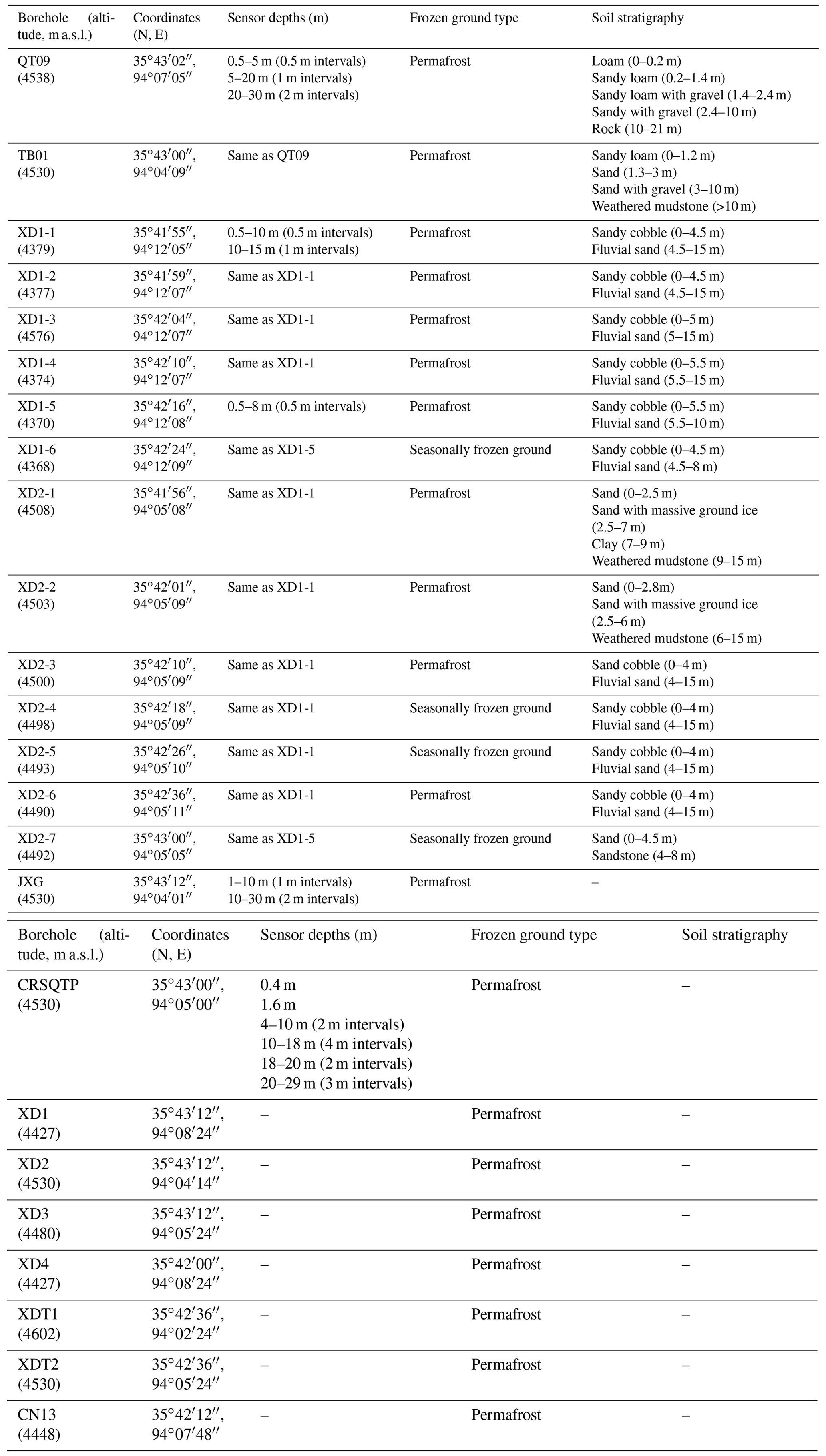
The symbol “–” is field-observed frozen ground types collected from previously published literature (Wang et al., 2000; Jin et al., 2000, 2006; Cheng and Wu, 2007).

Table A2 Calibration thermophysical parameters of different soil layers used for soil temperature modeling.

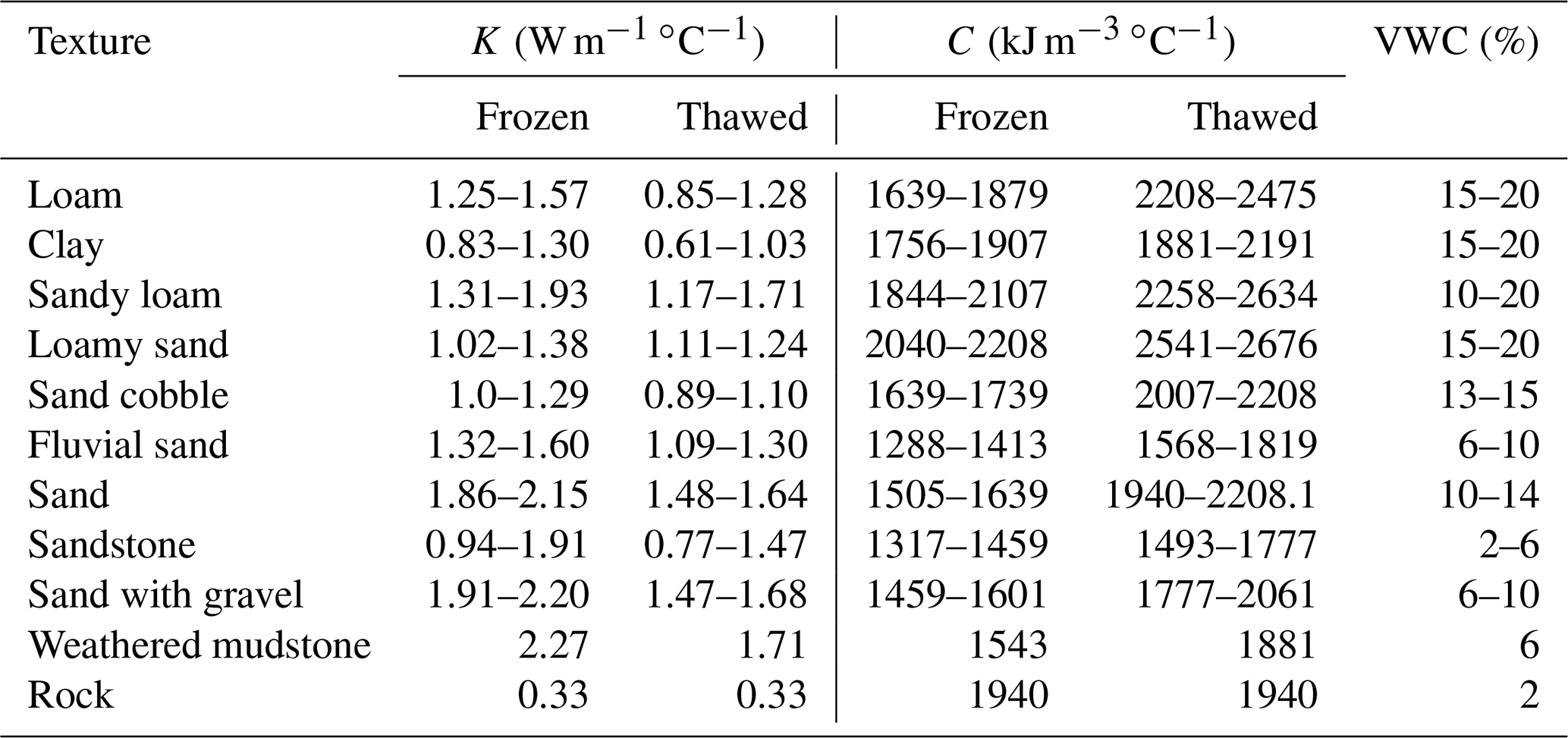
Note: K is the thermal conductivity; C is the volumetric heat capacity; VWC represents total volumetric water/ice content. Soil texture information was collected from Luo et al. (2018) and Liu et al. (2020), and the values of thermal conductivity and heat capacity are from the Construction of the Ministry of PRC (2011) and Yershov (2016) and are finely adjusted during the calibration; water content was determined by the soil samples of the borehole cores combined with the observation dataset vicinity of QT09 and the ground ice distribution maps from Zhao et al. (2010a).

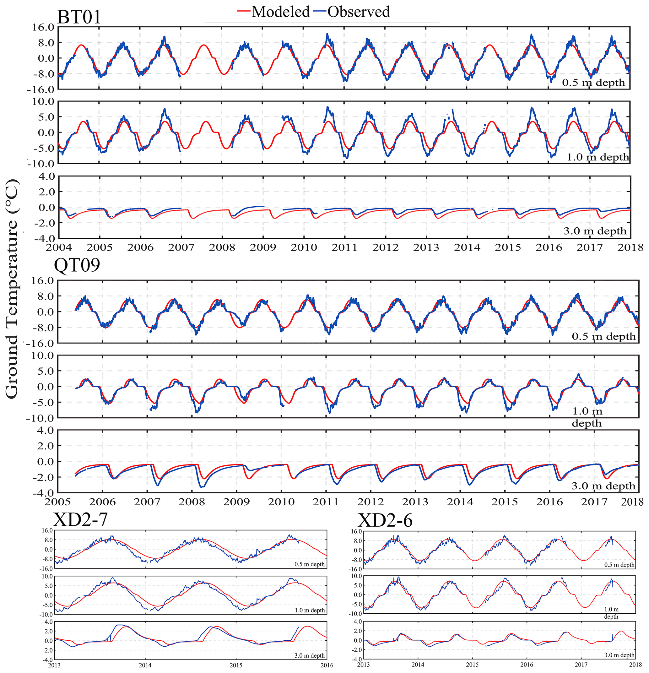
Figure A1 Comparison of the simulated (red lines) to observed (blue lines) daily mean ground temperature at 0.5, 1.0, and 3.0 m depth in four calibration boreholes (BT01, XD2-7, QT09, and XD2-6) during the observation period (there were some data gaps due to temperature probe failure in some years; at BT01, the data gaps in the record mainly occurred at 0.5–15 m in 2007–2008 and at 15–30 m during 2005–2007 and 2011–2018; at QT09, observations at 15–30 m of 2006–2008, 2011–2013, and 2015–2018 are not available; at XD2-6, the data gap in the record is in 2016–2017).

Figure A2 Same as Fig. 2 but for the daily mean ground temperature at 8, 15, and 30 m.

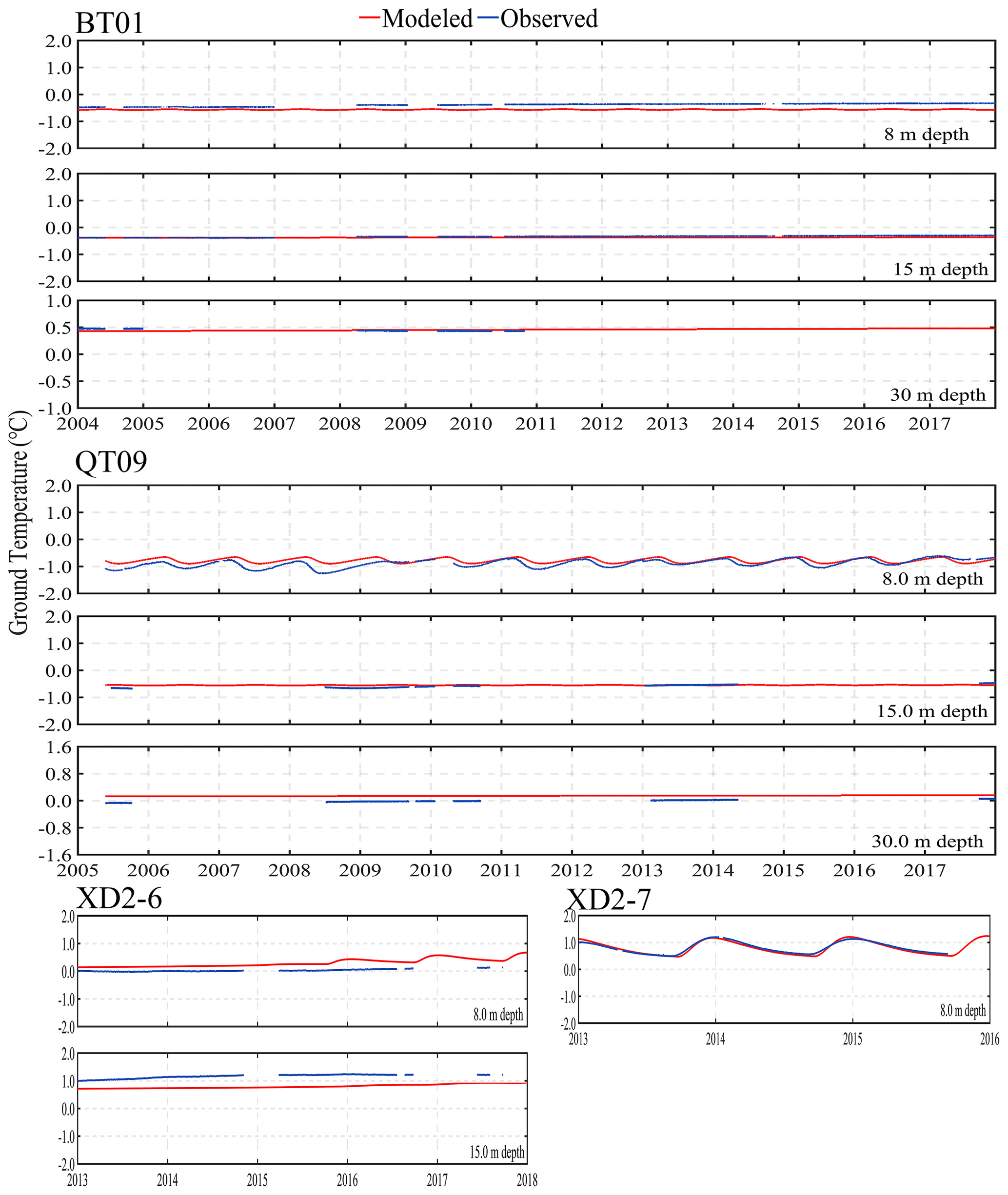
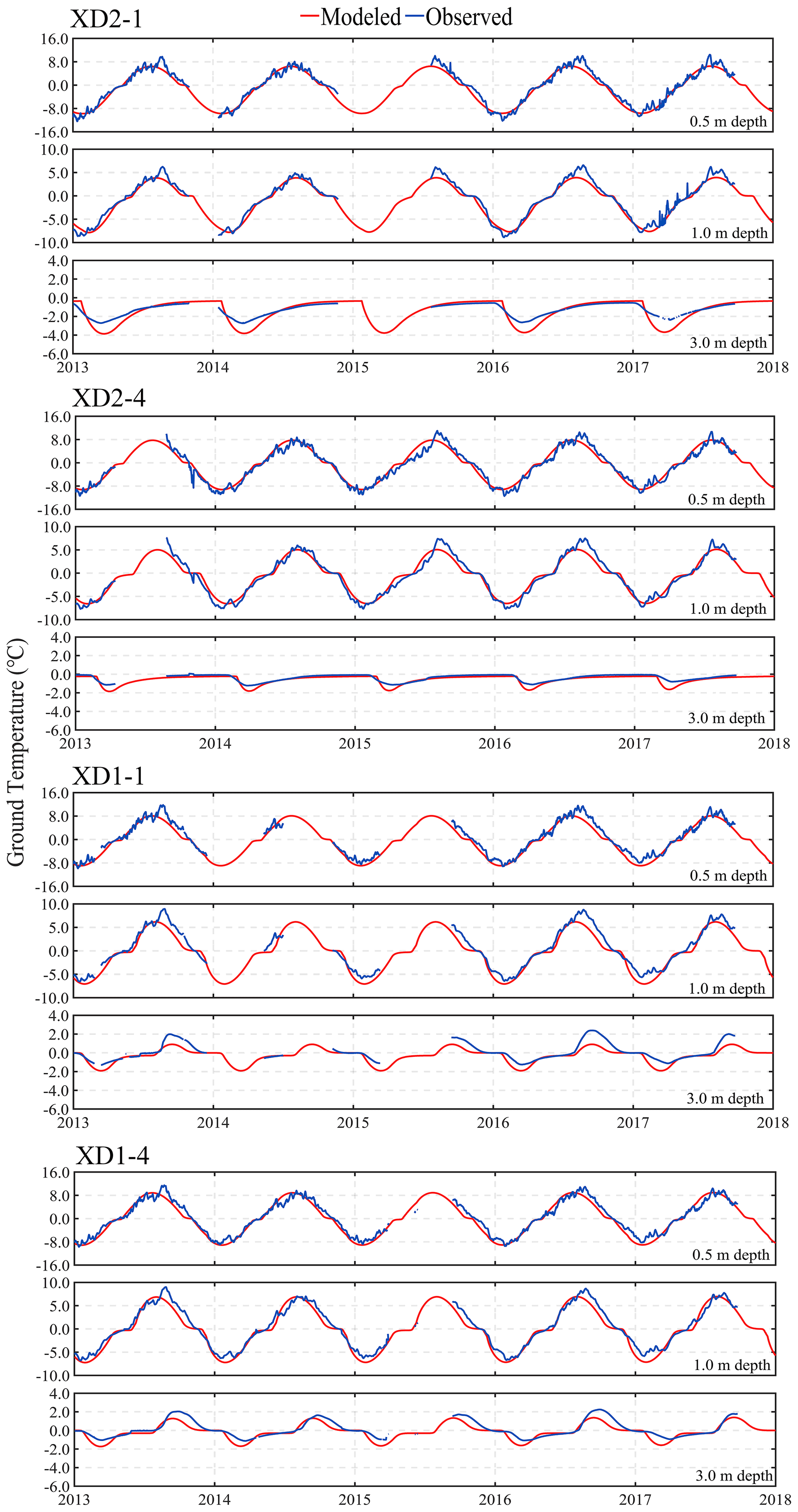
Figure A3 Comparison of the simulated (red lines) to observed (blue lines) daily mean ground temperature at 0.5, 1.0, and 3.0 m depth in four validation boreholes (XD2-1, XD2-4, XD1-1, and XD1-4) during the observation period from 2013 to 2018 (there were some data gaps due to temperature probe failure in some years; at XD2-1, the data gaps in the record mainly occurred at 0.5–3.0 m in the first half of 2015; at XD1-1, the data gap in the record is at 0.5–3.0 m in 2014–2015 and at 8–15 m during 2013–2015; at XD1-4, the data gap in the record is in the first half of 2015).

Figure A4 Same as Fig. 4 but for daily mean ground temperature at 8 and and 15 m.