the Creative Commons Attribution 4.0 License.
the Creative Commons Attribution 4.0 License.
 | 11 Nov 2022
The contribution of Humboldt Glacier, northern Greenland, to sea-level rise through 2100 constrained by recent observations of speedup and retreat
Matthew J. Hoffman
Mauro Perego
Stephen F. Price
Ian M. Howat
Humboldt Glacier, northern Greenland, has retreated and accelerated through the 21st century, raising concerns that it could be a significant contributor to future sea-level rise. We use a data-constrained ensemble of three-dimensional higher-order ice sheet model simulations to estimate the likely range of sea-level rise from the continued retreat of Humboldt Glacier. We first solve for basal traction using observed ice thickness, bed topography, and ice surface velocity from the year 2007 in a PDE-constrained (partial differential equation) optimization. Next, we impose calving rates to match mean observed retreat rates from winter 2007–2008 to winter 2017–2018 in a transient calibration of the exponent in the power-law basal friction relationship. We find that power-law exponents in the range of – – rather than the commonly used –1 – are necessary to reproduce the observed speedup over this period. We then tune an iceberg calving parameterization based on the von Mises stress yield criterion in another transient-calibration step to approximate both observed ice velocities and terminus position in 2017–2018. Finally, we use the range of basal friction relationship exponents and calving parameter values to generate the ensemble of model simulations from 2007–2100 under three climate forcing scenarios from CMIP5 (two RCP8.5 forcings, Representative Concentration Pathway) and CMIP6 (one SSP5-8.5 forcing, Shared Socioeconomic Pathway). Our simulations predict 5.2–8.7 mm of sea-level rise from Humboldt Glacier, significantly higher than a previous estimate (∼ 3.5 mm) and equivalent to a substantial fraction of the 40–140 mm predicted by ISMIP6 from the whole Greenland Ice Sheet. Our larger future sea-level rise prediction results from the transient calibration of our basal friction law to match the observed speedup, which requires a semi-plastic bed rheology. In many simulations, our model predicts the growth of a sizable ice shelf in the middle of the 21st century. Thus, atmospheric warming could lead to more retreat than predicted here if increased surface melt promotes hydrofracture of the ice shelf. Our data-constrained simulations of Humboldt Glacier underscore the sensitivity of model predictions of Greenland outlet glacier response to warming to choices of basal shear stress and iceberg calving parameterizations. Further, transient calibration of these parameterizations, which has not typically been performed, is necessary to reproduce observed behavior. Current estimates of future sea-level rise from the Greenland Ice Sheet could, therefore, contain significant biases.
- Article
(7445 KB) - Full-text XML
-
Supplement
(5193 KB) - BibTeX
- EndNote


The Greenland Ice Sheet (GrIS) could contribute up to 30 cm to global mean sea level in the 21st century, but uncertainty in the magnitude of sea-level rise (SLR) under a given emissions scenario exceeds 50 % (Goelzer et al., 2020; Edwards et al., 2021). Thus, a better understanding of the processes driving past and present retreat is necessary to reduce uncertainties in forecasts of GrIS mass loss. The retreat and acceleration of marine-terminating outlet glaciers has contributed roughly half of the net mass loss from the GrIS since the early 1990s, while increasingly negative surface mass balance has contributed the remaining half (IMBIE Team, 2019). The retreat of these outlet glaciers from their 20th century extents may be due to increased access of warm Atlantic Water to glacier termini from 1998–2007 (Wood et al., 2021). However, outlet glaciers experienced substantial thinning from 1985–2000, prior to the onset of rapid terminus retreat, with total ice discharge through outlet glaciers increasing rapidly by 14 % around the year 2000 (King et al., 2020). This step increase in discharge was sufficient to shift the GrIS into a state of negative mass balance, with the future annual probability of net mass gain estimated at around 1 % (King et al., 2020). While increased solid ice discharge is expected to remain a primary contributor to SLR from the GrIS over the course of this century (Choi et al., 2021), the precise mechanisms responsible for observed retreat and increased discharge remain poorly understood (King et al., 2020). Compounded with the wide range of polar warming predicted by climate models, this limits the precision of model-based estimates of future SLR (Barthel et al., 2020; Goelzer et al., 2020; Edwards et al., 2021; Payne et al., 2021). Thus, a process-based understanding of recent changes at the scale of individual outlet glaciers and estimates of the future retreat consistent with these changes is necessary in order to make precise and accurate estimates of the future SLR contribution of ice dynamics from the GrIS.
Despite widespread retreat of outlet glaciers of the northern GrIS, the velocity response has varied significantly from glacier to glacier (Hill et al., 2018). However, mass loss could accelerate in the future as glaciers retreat over beds that deepen inland, leading to a positive feedback known as the marine ice sheet instability that drives unstable retreat (Weertman, 1974; Schoof, 2007). Humboldt Glacier (Fig. 1) is one of the largest of the northern GrIS outlet glaciers and the widest outlet glacier of the GrIS, with a calving front almost 100 km across. It contains enough ice to raise global mean sea level by 19 cm if melted entirely (Rignot et al., 2021). Humboldt has lost the greatest area of grounded ice since 1992 of any GrIS outlet glacier (Box and Decker, 2011; Wood et al., 2021), with retreat concentrated almost entirely along the fast-flowing northern section of its marine terminus (Fig. 1; Carr et al., 2015). This northern section of the terminus is underlain by a deep basal trough that extends >70 km towards the ice sheet interior, sections of which deepen inland, raising concerns that Humboldt Glacier could be entering a phase of rapid, runaway retreat (Carr et al., 2015). The wide calving front and complex bed geometry of Humboldt Glacier make it particularly difficult to predict its future dynamical response to environmental changes. Furthermore, recent marine bathymetric surveys along the glacier terminus have shown that the glacier bed is up to 200 m deeper than previously thought (Rignot et al., 2021), indicating both that Humboldt Glacier is exposed to more oceanic heat and that previous modeling studies (Carr et al., 2015; Goelzer et al., 2020; Choi et al., 2021) may be hampered by inaccurate bed geometry.
In this paper, we use a three-dimensional, higher-order, thermomechanically coupled ice sheet model (Hoffman et al., 2018) to estimate the SLR contribution from Humboldt Glacier from 2007–2100 and assess sources of uncertainty. From an optimized initial condition, we perform hindcasting simulations from winter 2007–2008 to winter 2017–2018 to calibrate model parameters against observed changes at Humboldt Glacier. We first calibrate the basal friction law exponent using an imposed retreat rate. We then tune an iceberg calving parameterization using the range of calibrated basal friction law exponents. Next, we use the set of tuned model parameters in a perturbed parameter ensemble of 24 simulations to the year 2100 to estimate the likely range of SLR from Humboldt Glacier forced by three climate projections based on RCP8.5 (Representative Concentration Pathway) and SSP5-8.5 (Shared Socioeconomic Pathway) emissions scenarios. Finally, we explore additional sources of uncertainty in a set of sensitivity experiments that examine the impacts of assumptions about iceberg calving, oceanic melt, and bed topography. The perturbed parameter ensemble explores the parameter space that we are able to calibrate against observations, namely basal traction and iceberg calving, and represents our best estimate of 21st century SLR from Humboldt Glacier. The sensitivity experiments are used to validate modeling choices and explore processes and characteristics that we cannot calibrate within our framework, such as submarine melt, ice-shelf collapse, maximum calving rates (which are likely much greater than anything in the observational period), and bed topography.
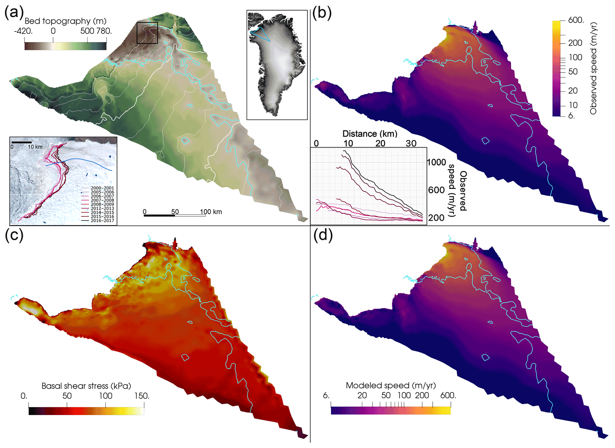
Figure 1Observations and optimization of Humboldt Glacier for the initial condition in the year 2007. (a) BedMachine v4 bed topography (Morlighem et al., 2017; Morlighem, 2021) interpolated onto the 1–10 km regional mesh. Cyan contour indicates bed topography at sea level in all panels. Black contour denotes ice edge. The 250 m thickness contours are shown in white, with thick contours marking 1000 m intervals. Inset on the upper right shows the location of our model domain in light blue, over a hillshade image from Howat et al. (2014). Inset on the lower left shows USGS Landsat imagery of the northern section of the marine terminus within the black box (Howat, 2017), with terminus positions from 2000 to 2017 (Moon and Joughin, 2008; Joughin et al., 2017). (b) Observed 2007–2008 ice surface velocity (Joughin et al., 2010, 2018) on a logarithmic color scale, interpolated onto our regional mesh. The inset on the lower left shows velocity transects over time along the approximate flowline marked in blue in the lower-left inset of panel (a), using the same color scale. (c) Magnitude of basal shear stress for our 2007 optimized initial condition and (d) the resulting modeled ice surface velocities. Panels (b), (c), and (d) are trimmed to the 2007 ice extent, while panel (a) shows the entire domain. Errors between optimized and observed velocities are shown in Fig. S1.
2.1 Ice sheet model
We model the evolution of Humboldt Glacier over a regional domain on a 1–10 km variable resolution mesh (Fig. 1; 18 544 cells with 10 vertical levels) using the MPAS-Albany Land Ice (MALI; Model for Prediction Across Scales) model (Hoffman et al., 2018). MALI is a thermodynamically coupled, finite-element and finite-volume code that solves the first-order Stokes approximation for momentum balance in three dimensions (Blatter, 1995; Pattyn, 2003), using Nye's generalization of Glen's flow law as the constitutive law (Glen, 1955; Nye 1957). We impose Dirichlet velocity boundary conditions around the domain edges using the observed 2007–2008 winter surface velocity from Joughin et al. (2018). This prevents the possibility of catchment boundary migration, but this is a minor error over the timescales considered here. For basal friction, we use an effective pressure-dependent power-law relationship of the form , where τb is basal shear stress, N is the effective pressure at the glacier bed, μ is the spatially varying friction parameter, u is the velocity at the glacier bed, and 0<q≤1 is a power-law exponent discussed in more detail below (Budd et al., 1979, 1984). N is calculated as ice overburden pressure minus subglacial water pressure with the commonly used simple assumption of perfect connectivity between the subglacial hydrologic system and the ocean (e.g., Vieli et al., 2001; Seroussi et al., 2013; Asay-Davis et al., 2016; Morlighem et al., 2019). N evolves based on ice geometry in all simulations. For the energy balance, we use an enthalpy formulation, as described by Hoffman et al. (2018) and based on Aschwanden et al. (2012). We use a map of basal heat flux from Shapiro and Riztwoller (2004).
2.2 Data sources and optimized initial condition
We use a PDE-constrained (partial differential equation) adjoint optimization method to solve for the basal friction parameter μ to create our initial condition for the year 2007. This procedure minimizes the sum of the modeled velocity misfit to observations and a regularization term (Figs. 1, S1; see also Perego et al., 2014) while constraining the ice velocity and temperature to satisfy the coupled first-order Stokes and enthalpy equations. We set for the optimization, but we later tune this value to find the values that best match observed changes in velocity during retreat in a set of forward runs, as described further in Sect. 2.3. Ice thickness and bed topography are from BedMachine Greenland v4 (BMv4; Morlighem et al., 2017; Morlighem, 2021), with a nominal date of 2007. Observed 2007–2008 winter ice velocities and their uncertainties are taken from Joughin et al. (2018), with areas of missing velocity filled using a composite 1995–2015 velocity map (Joughin et al., 2016, 2018). While the composite 1995–2015 velocities do not correspond to a given year, the data gaps are found only in slow-moving ice far from the marine terminus, and thus this has a negligible effect on our results. The initial ice extent from BMv4 is trimmed slightly to match the ice margin as defined in the velocity datasets. Surface mass balance, surface air temperature, subglacial runoff, and ocean thermal forcing fields are taken from the Ice Sheet Model Intercomparison Project for CMIP6 (ISMIP6; Coupled Model Intercomparison Project phase 6) (Nowicki et al., 2020; Slater et al., 2020), which provides these outputs from a number of earth system models. We use the MIROC5 (Model for Interdisciplinary Research on Climate version 5) RCP8.5 and HadGEM2 (Hadley Centre Global Environment Model version 2) RCP8.5 products recommended by ISMIP6 to represent medium and strong anthropogenic forcing, respectively (Barthel et al., 2020; Slater et al., 2020; see their Fig. 10b). We also include the CNRM-CM6 (Centre National de Recherches Meteorologiques Climate Model version 6) SSP5-8.5 forcing to represent the midrange of the few available CMIP6 forcings, which are known to be among those with the highest climate sensitivity in CMIP6 (Payne et al., 2021). Climate forcing time series are shown in Fig. 2.
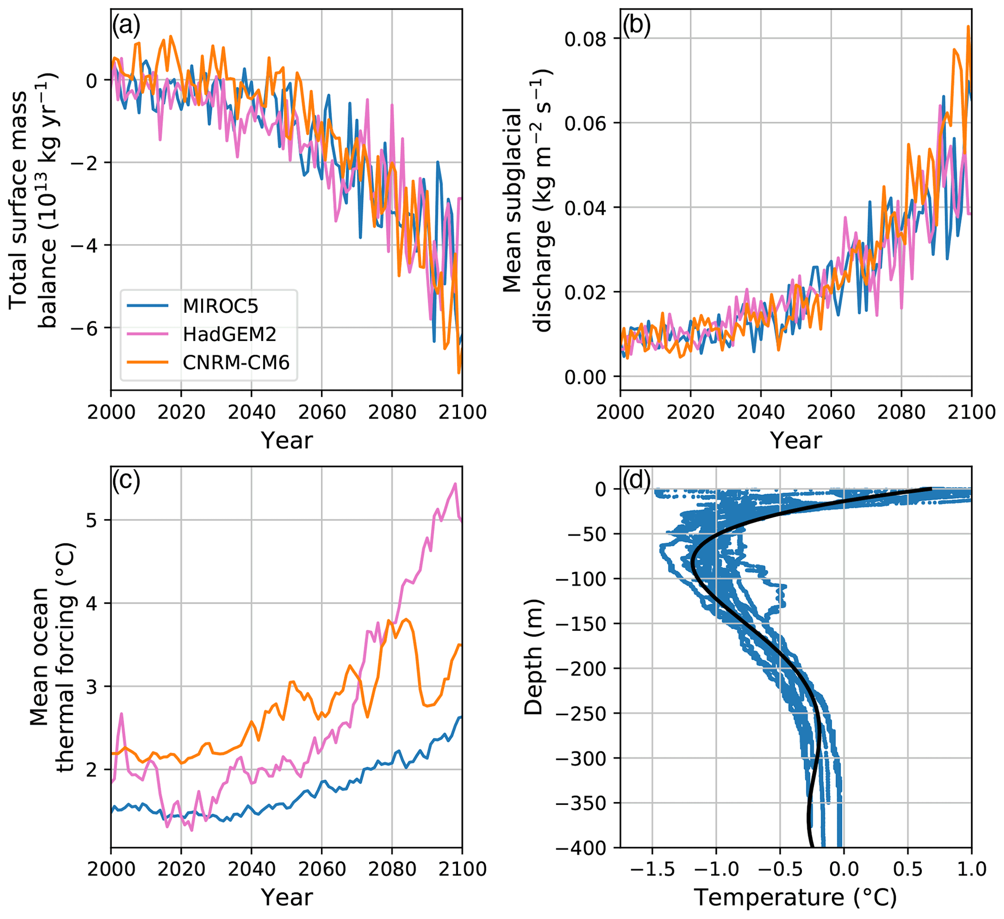
Figure 2(a–c) Time series of climate forcings from MIROC5, HadGEM2, and CNRM-CM6 earth system models, provided by ISMIP6. Values in panels (a) and (b) were calculated by summing or averaging over the ice extent in the 2007 initial condition, and so values in these plots do not take into account the retreating ice margin. The values in panel (c) were calculated using the area between the initial ice front and the most retreated grounding-line position in our perturbed parameter ensemble, where the bed is below sea level. The total and mean values are depicted here for illustration, but the full time-varying, two-dimensional fields are used to force the simulations. (d) Ocean temperature observations (blue) from Oceans Melting Greenland, used for creating three-dimensional ocean thermal forcing fields from the two-dimensional fields provided by ISMIP6. Black curve shows polynomial fit.
2.3 Tuning of the basal friction law exponent
Our optimization provides basal shear stress and velocity for the initial condition, but the evolution of these fields depends on the value of the basal friction relationship exponent, q, which is not known a priori and cannot be determined from a single snapshot in time (Gillet-Chaulet et al., 2016; Joughin et al., 2019). Thus, to find the appropriate range of values of q, we recalculate the friction parameter μ for and evaluate each case against observed velocities after a decade of forward integration. The friction parameter is recalculated for each assumed value of q with values from the 2007 initial condition using the constraint of basal traction from the optimized initial condition:
where NIC is effective pressure at the initial condition; μopt and uopt are, respectively, the friction parameter and basal sliding speed from the optimization using ; and μq is the friction parameter corresponding to the assumed value of q. Solving for μq, we obtain . This relation yields very nearly the same velocity as the optimization for the initial condition (Fig. S2), which validates our recalculation of μ. For each value of q considered, we impose a spatially variable calving front retreat rate that matches the mean observed retreat rate between the 2007–2008 and 2017–2018 ice extents from Joughin et al. (2018). We perform the calibration over a full decade of change to take advantage of the largest signal of velocity change available. This also avoids calibrating to noisy interannual variability and aliasing to temporal gaps in the data; for instance, the data gap between 2008–2009 and 2012–2013 (Fig. 1) means that we cannot say whether the glacier retreated monotonically during this period or if it retreated and then readvanced to the 2012 margin. Aside from the imposed calving rate, the only other forcing in this step is the MIROC5 RCP8.5 surface mass balance. The imposed calving rate represents the sum of retreat due to calving and submarine melting in reality, the individual components of which are not readily available from observations. The ice thickness and velocity fields evolve in response to the imposed retreat.
We calculate the root mean square error in the modeled velocities from the observed 2017–2018 winter velocities divided into four bands (all velocities, as well as 0–300, 300–600, and >600 m yr−1) to determine an appropriate range of values for q (Fig. 3). The choice to use multiple velocity bands was motivated by the need to match the large observed change in the fast-flowing region that is very spatially limited compared with the much larger slow-flowing region of the glacier. There is a trade-off between matching 2017–2018 velocities in fast- and slow-flowing areas when using a single value of q. Using only the global misfit to observed velocities would suggest ; however, this leads to a very poor fit in the region near the terminus with high velocities and large changes. We find that yields reasonable agreement to the 2017–2018 velocities in the fastest-flowing parts of the glacier, without causing problematic amounts of acceleration elsewhere. Thus, we use values of and for q in our forward simulations. While the definition of the velocity bands and resulting choice of the best values of q are somewhat subjective, we tested the sensitivity of the calibration to our choice of velocity bands and found it to be relatively insensitive (Fig. S3). We also performed a separate set of calibration runs following the same methodology with the 2015–2016 velocities and margin, which further corroborates our choice of (Fig. S4).
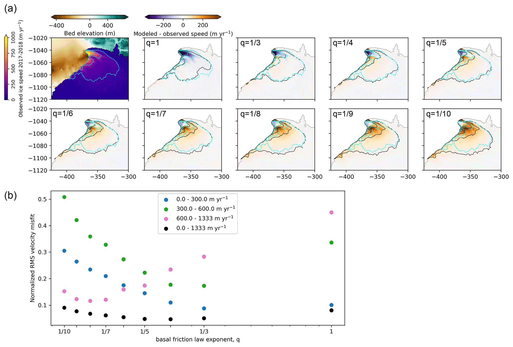
Figure 3(a) Observed 2017–2018 winter velocity and modeled deviation from observations using an imposed retreat rate to match the observed 2017–2018 margin for the range of basal friction law exponent values examined. Observed (cyan) and modeled (black) velocities are contoured at 100, 300, and 600 m yr−1. (b) Root mean square (RMS) velocity misfits between model and observation values normalized by the midpoint value of each velocity band for all basal friction law exponents examined. Velocity bands are defined using the observed 2017–2018 velocities.
2.4 Submarine melting parameterizations
We use separate parameterizations to represent submarine melting of grounded and floating ice. To represent melt undercutting where the marine terminus is grounded, we use the relationship (Rignot et al., 2016; Slater et al., 2020), where qm is the horizontal melt rate perpendicular to the calving front in meters per day, A=0.0003 mα dα−1 ∘C−β, h is water depth at the terminus in meters, qsq is subglacial runoff in meters per day, α=0.39, B=0.15 m d−1 ∘C−β, TF is ocean thermal forcing in degrees Celsius (taken from the ISMIP6 two-dimensional thermal forcings), and β=1.18.
In preliminary model runs, we found that the modeled glacier develops a sizable ice shelf by the middle of the 21st century in many simulations. Therefore, we also include a basal melt parameterization for floating ice developed for Antarctic ice shelves (Jourdain et al., 2020):
where m(x,y) is ice-shelf melt; γ0 is a tuning parameter with units of velocity, analogous to an exchange velocity; ρsw and ρi are densities of seawater and ice, respectively; cpwis the specific heat of seawater; Lf is the latent heat of fusion for ice; TF() is the thermal forcing at the ice-shelf base; and 〈TF〉draft∈shelf is the thermal forcing averaged over the whole ice shelf. Other studies have used melt formulations in which the relationship between sub-shelf melt and thermal forcing is linear (Choi et al., 2021) or weakly non-linear (Cai et al., 2017). However, the currently accepted theoretical formulation is for melt to be a quadratic function of thermal forcing (Holland et al., 2008), as we apply here.
We constructed three-dimensional ocean thermal forcing fields using all available conductivity–temperature–depth (CTD) and airborne-expendable conductivity–temperature–depth (AXCTD) measurements from the Oceans Melting Greenland campaign (OMG, 2019, 2020) within the bounding box [79.0∘ N, 70.0∘ W; 79.9∘ N, 64.0∘ W] between 2016 and 2020. First, we converted the temperature measurements to thermal forcing using the relationship , where . Here, TF is thermal forcing, T is measured temperature, Tfreeze is the freezing temperature of seawater, ∘C PSU−1 (practical salinity unit), Sref is a reference salinity of 34.4 PSU, b=0.0901 ∘C, ∘C m−1, and z is depth (Jenkins, 1991). We then fit a fifth-order polynomial to these data (Fig. 2d) to obtain TF at the top and bottom of the thermocline (80 and 250 m, respectively). We use four vertical ocean levels of depths 0, 80, 250, and 1000 m, for which the top two and bottom two are set to the same respective temperature values but TF is allowed to vary based on the pressure-dependence of Tfreeze. The model interpolates linearly between these levels based on ice-shelf draft. For each ISMIP6 ocean thermal forcing, this vertical relationship is then translated based on the two-dimensional thermal forcing, taken to be TF at the bottom of the thermocline (250 m depth). We then tune γ0 in the TF–melt relationship to obtain mean melt rates of 20 m yr−1 beneath floating ice in our initial condition. We find γ0 values of 30 246 m yr−1 for CNRM-CM6, 45 292 m yr−1 for HadGEM2, and 75 580 m yr−1 for MIROC5. For reference, Jourdain et al. (2020) found median γ0 values for Antarctica of 14 500 and 159 000 m yr−1 for their two calibration methods. In forward runs, this also produces mean melt rates of ∼ 20 m yr−1 over the period of winter 2007–2008 to winter 2017–2018, despite the evolving ice thickness. This tuning effectively normalizes the thermal forcing fields shown in Fig. 2 so that the relevant quantity for sub-shelf melt is the change in thermal forcing relative to 2007, while the relevant quantity for undercutting is the absolute value of thermal forcing. The mean melt rate of 20 m yr−1 was chosen as a representative value for sub-shelf melt near the grounding line of nearby Petermann Glacier (Cai et al., 2017) and may not be entirely appropriate for Humboldt Glacier; however, we view this as the best estimate available given the lack of ice-shelf melt rate estimates at Humboldt Glacier and the considerably smaller amount of floating ice. To investigate the sensitivity of our results to this choice of melt tuning, we include a set of forward simulations with ice-shelf melt tuned to 10 and 30 m yr−1.
2.5 Calving parameterizations
Development of significant floating ice is not typically expected in Greenland, and some modeling studies have required ice to calve as soon as it goes afloat (e.g., Morlighem et al., 2016). We find that removing all floating ice leads to too rapid retreat over the observed period, and therefore we do not require floating ice to calve immediately but instead use two calving parameterizations that each treat floating and grounded ice the same. The first is the von Mises stress calving parameterization of Morlighem et al. (2016): , where c is calving velocity, v is the depth-averaged ice velocity, σ is the depth-averaged tensile von Mises stress, and σmax is a yield stress that we treat as a tuning parameter. Thus, the calving rate exceeds the ice velocity for σ>σmax, causing the calving front to retreat. We use the same value of σmax for grounded and floating ice. Choi et al. (2021) found that the threshold stress needed to be as low as 150 kPa to match observed retreat for some Greenland outlet glaciers, which is far below estimates for the tensile strength of ice reported by Petrovic (2003), which range from 700 kPa to 3.1 MPa. We also find that very low values of σmax (≤ 200 kPa) are necessary to cause retreat at Humboldt Glacier. However, we find that this leads to a positive feedback in which increased velocity causes both increased calving and decreased basal friction due to thinning, which in turn causes higher velocities; this is exacerbated by the non-linear basal friction relationship. In preliminary forward runs, this led to unrealistic rates of calving and ice flow after ∼ 2030. We found it necessary to impose a 3 km yr−1 upper limit on the calving rate following Choi et al. (2018). While this is an ad hoc solution, it avoids the far more problematic effect of the positive feedback between velocity and calving rate. We explore the impact of this assumption in a sensitivity experiment described below.
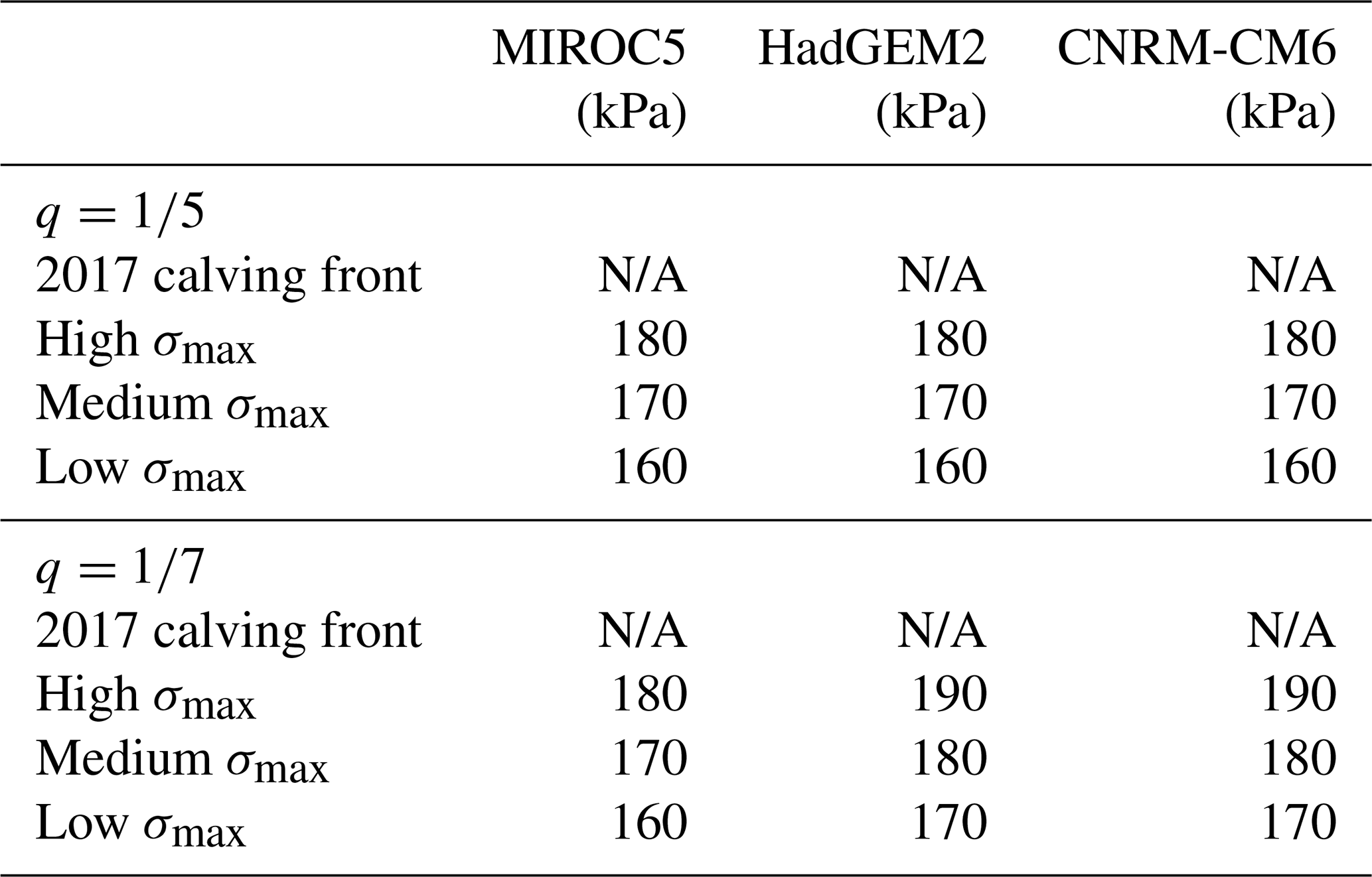
To tune the von Mises tensile threshold stress parameter, σmax, we ran the model from winter 2007–2008 to winter 2017–2018 with values of σmax of 150, 160, 170, 180, 190, and 200 kPa for all pairs of climate forcing and the calibrated basal friction law exponent ( and ). We compared the fit of the modeled ice margin position and velocity field to observations in 2017–2018 (Joughin et al., 2018). For each pair of climate forcing and the basal friction law, we chose three values of σmax for century-long projection runs. Values of σmax that minimized the misfit to observed surface velocities and ice front positions are in the range of 160–190 kPa (Fig. S5; Table 1). MALI lacks a sub-grid tracking scheme for the calving front; instead, the calving front is tracked as described by Hoffman et al. (2018), following the method of Albrecht et al. (2011) that includes a row of thin non-dynamic cells at the marine margin to conserve mass. The marginal dynamic cells are considered to be the calving front, and their stress and velocity values are used to calculate the local calving velocity. Calved ice is instantaneously removed from the domain. Submarine melting is active during the calving calibration runs.
We recognize that uncertainties and biases inherent in the calving parameterization could have a large impact on mass-loss projections. To address this, we also include a set of minimum mass-loss simulations, similar to those of Price et al. (2011), which branch off from the basal friction law exponent tuning runs in 2017. After the tuning run with an imposed retreat rate, we allow only enough calving to hold the glacier terminus at its 2017 position. The terminus may retreat behind this position due to surface mass balance and ocean thermal forcing, but no calving is active inward of the 2017 terminus. While this is not likely to be an accurate depiction of glacier retreat over the 21st century, we view it as a good estimate of a lower bound on mass loss, as we believe Humboldt Glacier is very unlikely to advance significantly beyond its 2017 position under the climate scenarios examined in this study.
2.6 Forward simulations
2.6.1 Control
For each pair of the basal friction law and climate forcing, we run a control simulation imposing only the mean 1960–1989 surface mass balance as a forcing, through the entire run from 2007–2100. There is no explicit calving or submarine melting, but ice that advances beyond the 2007 terminus is immediately melted away to avoid advance into regions of an unconstrained basal friction coefficient. This serves to quantify the mass loss and equivalent sea-level contribution from our model without climate forcing corresponding to the onset of rapid Greenland outlet glacier retreat around the year 2000 (King et al., 2020). We later subtract this mass loss from the simulations in the perturbed parameter ensemble discussed below to isolate mass loss and sea-level rise due to future climate changes rather than model drift or ongoing adjustment to historical climate.
2.6.2 Perturbed parameter ensemble
For each pair of climate forcing and the basal friction law, we perform four simulations from 2007–2100 (Table 1): (1) a minimum mass-loss scenario with time-varying surface mass balance and submarine melt forcing but with only enough calving to keep the glacier from advancing beyond the 2017–2018 margin (these runs branch off of the basal friction tuning runs described above in winter 2017–2018) and (2–4) three scenarios with the von Mises calving law, submarine melting, and surface mass balance forcing, using the three values of σmax that best match the observed retreat and speedup. In all runs, ice is again not allowed to advance past its 2007 margin to prevent advance onto areas of unconstrained basal friction, although this only has an effect early in the minimum mass-loss runs. We also include two simulations with q=1 using σmax=150 and 180 kPa for each climate forcing to illustrate the effect of tuning the power-law basal friction relationship; these linear basal friction law simulations should not be taken as estimates of SLR.
Table 1Runs conducted with the perturbed parameter ensemble, with σmax for all members using the von Mises stress parameterization. Calibration results to determine σmax are shown in Fig. S5. N/A: not applicable.
2.6.3 Sensitivity experiments
In addition to the main perturbed parameter ensemble, we include sensitivity experiments to explore the role of floating ice, maximum calving rates, and bed topography in the evolution of Humboldt Glacier. All sensitivity experiments use the intermediate value of σmax for the appropriate climate forcing–basal friction exponent pair (Table 1). The sensitivity experiments are summarized in Table 2.
In the first sensitivity experiment, we remove all floating ice starting in 2055 and thereafter require ice to calve as soon as it goes afloat, while keeping the von Mises calving law the same for grounded ice. We choose 2055 as the branch point because this is approximately when the surface mass balance of the ice sheet is expected to become persistently negative (Noël et al., 2021); we thus remove floating ice as a crude representation of the hydrofracturing of the ice shelf as surface ponding drastically increases, as has been observed in Antarctica (e.g., Scambos et al., 2000; Banwell et al., 2013). While hydrofracture could become an important process earlier or later than 2055, this tipping point provides a reasonable choice of timing for this sensitivity experiment that still allows us to match observations early in the simulation. This experiment was done for all climate forcings and both basal friction law exponents.
In the second experiment, we examine the sensitivity of our century-scale projections to the assumed mean 2007–2018 sub-shelf melt rate by tuning sub-shelf melting to 10 and 30 m yr−1 instead of 20 m yr−1. This experiment was done for the CNRM and HadGEM2 climate forcings as the bounding cases of mass loss in our perturbed parameter ensemble (Fig. 5), with both basal friction law exponents.
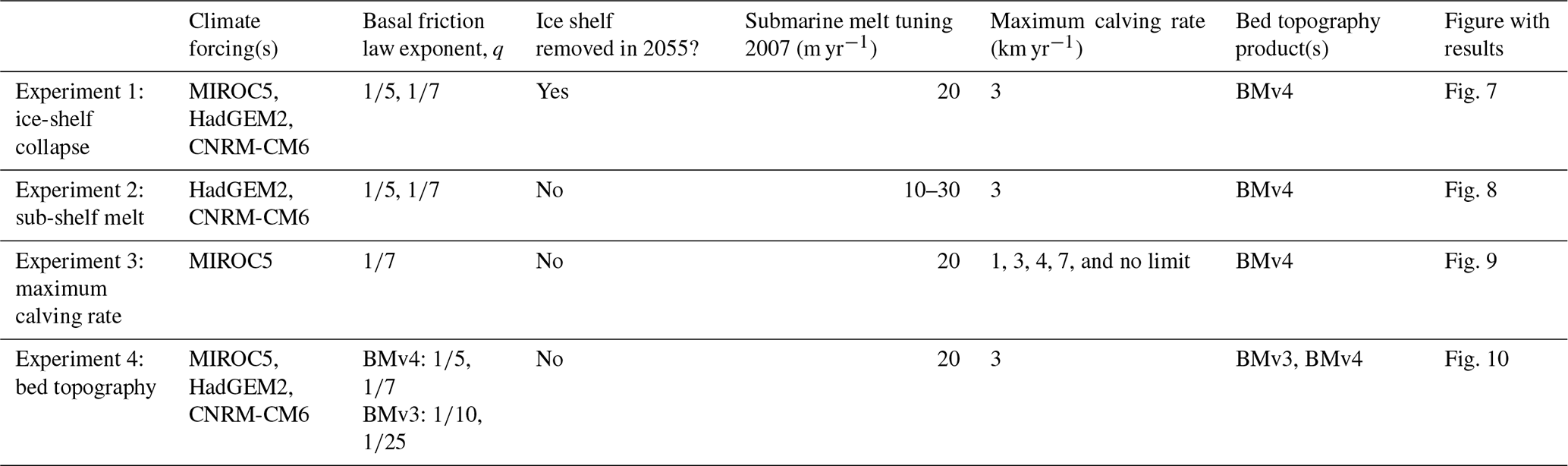
In the third sensitivity experiment, we explore the impact of our choice of 3 km yr−1 for the maximum calving rate by including a set of simulations with 1, 5, and 7 km yr−1 upper limits, as well as a simulation with no limit imposed on calving rates. These runs were done with the MIROC5 climate forcing, .
In the fourth sensitivity experiment, we explore the impact of uncertainty in bed topography by repeating a set of runs using BedMachine version 3 (Morlighem et al., 2017; Morlighem, 2017) for comparison with our main results using BedMachine version 4. This is motivated by the ∼ 20 %–25 % uncertainties in ice thickness reported near the northern portion of the marine margin in BedMachine version 4. While the differences between versions 3 and 4 are slightly larger than the uncertainty within version 4, we use this as a bounding case that still uses a data-constrained, mass-conserving bed that has been used in previous studies (Goelzer et al., 2020; Choi et al., 2021). We repeat both the optimization for the friction parameter μ and the basal friction law exponent tuning procedure described above, applied instead to the bed topography from BedMachine version 3. We then run forward simulations from 2007–2100 for all three climate forcings and both basal friction law exponents.
3.1 Perturbed parameter ensemble
3.1.1 Sea-level contribution
The results of the perturbed parameter ensemble that constitutes our SLR estimates to 2100 are shown in Figs. 4 and 5. All simulations predict significant retreat in the northern section of the terminus (Fig. 4). Grounding-line retreat in our minimum mass-loss simulations with a 2017 calving front position is nearly as extensive as those using von Mises stress calving, with variation due to climate forcing and the basal friction law exponent. We find that for our fixed 2017 calving front scenarios, the model predicts 5.2–6.1 mm SLR by 2100, relative to our control simulations (∼ 0.85–1.4 mm). In these minimum mass-loss simulations, almost all the variability in SLR is due to the choice of climate forcing, with MIROC5 and CNRM predicting ∼ 5.2–5.7 mm SLR by 2100 and HadGEM2 predicting 5.8–6.1 mm SLR by 2100. The two values of the basal friction law exponent ( and ) predict very similar SLR rates and totals over the whole century within each climate forcing. Thus, for our fixed 2017 calving front scenarios, the calibration of the basal friction law has successfully constrained the exponent to a range where the results are no longer sensitive to its uncertainty.
Using the von Mises stress calving parameterization leads to greater variability and higher mass loss than the assumption of minimal calving after 2017. Our von Mises calving scenarios predict 6.2–8.7 mm SLR from 2007–2100 relative to our control simulations, with variability due to stress threshold tuning, the basal friction law exponent, and atmosphere and ocean forcing (Fig. 5). We also include a set of six runs with a linear basal friction law (q=1) and low and high calving sensitivities to illustrate the importance of tuning the exponent to match observations. When compared with the linear basal friction law, our runs with tuned basal friction exponents predict up to twice as much SLR by 2100.
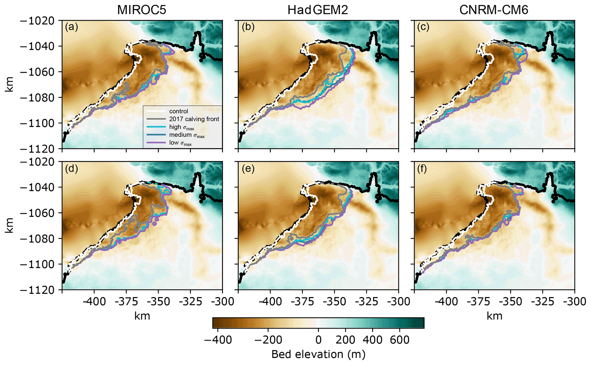
Figure 4Grounding-line position at 2100 for all members of the perturbed parameter ensemble. Results are shown for (a–c) and (d–f) for the basal friction law exponent. Black curves represent the initial ice extent in 2007. Grounding lines from control runs are shown in white. Curve colors represent calving scenario.
3.1.2 Ice-shelf growth
We find that a significant amount of floating ice grows by the mid-century in all ensemble members using von Mises stress calving and late in the century for most minimum mass-loss calving scenarios (Figs. 5, S7, S8). This is not generally anticipated for Greenland, where two out of only five total ice shelves have collapsed since the 1990s (Mottram et al., 2019) and model results predict the loss of the nearby Petermann Glacier ice shelf in the coming decades (Åkesson et al., 2021). Under the HadGEM2 climate forcing, the ice shelf is lost by the end of the century, but significant floating ice persists until 2100 for the majority of runs with MIROC5 and CNRM-CM6 climate. As expected, the volume of the ice shelf is dependent on calving tuning and the basal friction law as well as climate, with greater volumes of floating ice predicted in runs with higher σmax and a more plastic bed rheology (). However, in cases with HadGEM2 climate forcing, an increase in ice-shelf basal melting due to warmer ocean temperatures beginning in the early 2070s (Figs. 2, 6) removes the majority of floating ice within a decade. This period also corresponds with an increase in the rate of SLR contribution around 2075 for HadGEM2 climate (Fig. 5) as the surface mass balance over grounded ice also becomes increasingly negative (Fig. 6). We further explore the impact of this floating ice in two sets of sensitivity experiments, described below (Sect. 3.2.1, 3.2.2).

Figure 5(a–c) Projections of volume loss and equivalent global mean sea-level rise from the perturbed parameter ensemble of 21st century simulations of Humboldt Glacier. Curves represent the basal friction law exponent of (solid), (dashed), and q=1 (dotted) for comparison. The corresponding control run has been subtracted from each curve. (d–f) Projections of the total volume of floating ice from the same simulations as the top row. Curve colors denote the calving scenario. Values of σmax corresponding to low, medium, and high thresholds are found in Table 1.
3.1.3 Mass budgets
We next investigate the contributions of individual processes (calving, basal and submarine melting, grounding-line flux, and surface mass balance) to the evolution of the total volume of both grounded and floating ice. Figure 6 shows the cumulative mass budgets for grounded (top row) and floating (bottom row) ice for the von Mises stress calving runs from our perturbed parameter ensemble through time. For grounded ice, we find that submarine melt undercutting at the grounded terminus contributes negligibly to the mass budgets over the 21st century, despite potentially being the dominant driver of recent retreat (Rignot et al., 2021). Undercutting does play a role in simulated mass loss over the historical period but is not the dominant mode of mass loss; however, melt at the base of floating ice is also significant over this period. Because floating ice early in the model simulations is very close to the floatation thickness, our model could be overestimating ice-shelf melt and underestimating undercutting at the grounded front. We ran a set of six simulations from 2007–2021 with undercutting deactivated and found that the total calving flux is significantly decreased compared with simulations that include undercutting (Fig. S9). This is because the grounded ice margin is close to its floatation thickness, so a small amount of undercutting causes the grounded margin to go afloat, which causes increased velocity and tensile stress, which in turn cause higher calving rates. Thus, while undercutting does not contribute significantly to the mass budget directly, its control on calving makes it an important process governing the retreat of Humboldt Glacier over the observational period.
Grounding-line flux is the largest contributor to total grounded ice loss in almost all simulations, but it is overcome by surface mass balance for the cases using HadGEM2 climate and the basal friction law exponent. Calving from the grounded terminus is a significant contributor to grounded ice loss in all simulations, while melting at the base of grounded ice is a negligible term in the mass budget. The value of the basal friction law exponent makes the largest difference in grounding-line flux and a minor difference in calving from the grounded terminus; it makes almost no difference in surface mass balance, basal melting, or undercutting contributions to the budget. Net surface mass balance contribution is almost entirely negative for MIROC5 and HadGEM2, while the CNRM-CM6 net surface mass balance is positive until the mid-2060s, after which it becomes steeply negative. Surface mass balance contributes ∼ 3.1 mm SLR for CNRM-CM6, ∼ 3.7 mm SLR for MIROC5, and ∼ 4.1 mm SLR for HadGEM2 climate forcing. Other terms in the grounded budget in Fig. 6 should not be interpreted directly in terms of SLR because much of the ice lost by calving, grounding-line flux, and undercutting is not above flotation.
Calving and sub-shelf melting dominate mass loss from floating ice. Calving is dominant early in the century, while sub-shelf melting generally reaches a similar magnitude by the end of the century. Surface mass balance plays a minor role on floating ice. We observe higher sub-shelf melting, calving, and grounding-line flux in the runs than in the runs, but these roughly balance out to give similar net volume change for floating ice between the two basal friction law exponents.
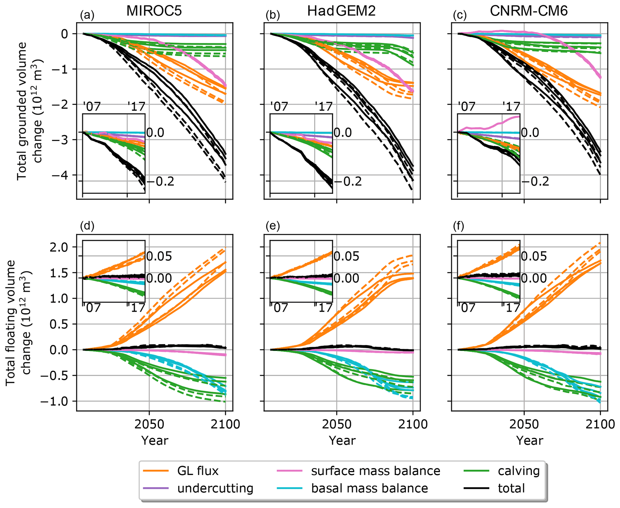
Figure 6Mass budgets for (a–c) grounded and (d–f) floating ice for all runs using von Mises stress calving. Colors indicate components of the budget, while line styles indicate the value of the basal friction law exponent (solid: ; dashed: ). Insets in each panel show the 2007–2021 period. GL flux: grounding-line flux.
3.2 Sensitivity experiments
3.2.1 Removal of floating ice
We find that the presence of floating ice significantly reduces mass loss from Humboldt Glacier for all three climate forcings and both basal friction law exponents (Fig. 7). Simulations with floating ice removed in 2055 and prevented from regrowth predict 1–2 mm (up to ∼ 25 %) more SLR by 2100 than the counterpart simulations within the main perturbed parameter ensemble, due to a combination of loss of buttressing and increased calving from the grounded ice margin. Removing floating ice at the beginning of the simulation would likely lead to greater SLR contribution, but it would not be possible to match the observed retreat and speedup.
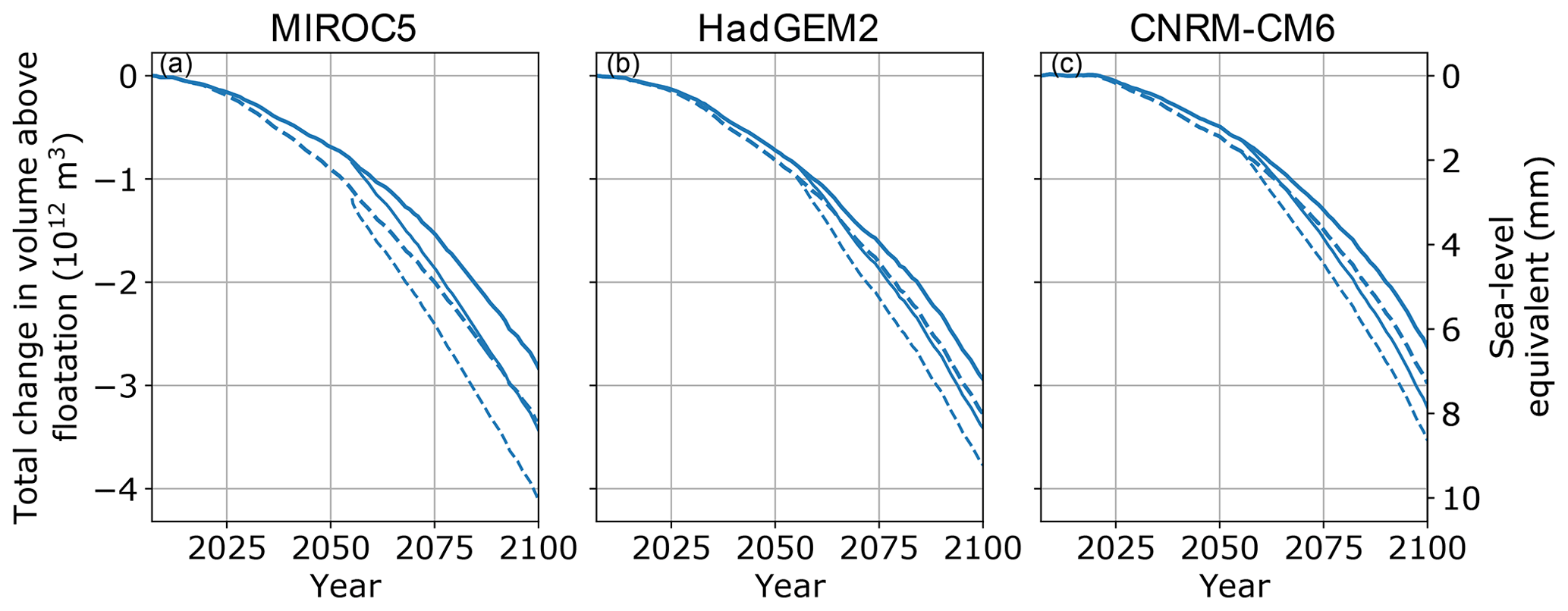
Figure 7Results of the sensitivity test in which floating ice is removed in 2055 and not allowed to regrow. As in other figures, the solid and dashed curves represent and , respectively. Thicker upper curves are the runs with floating ice maintained (i.e., same as blue curves in Fig. 5); thinner lower curves are with floating ice removed.
3.2.2 Sub-shelf melt tuning
Figure 8 shows the results of our sensitivity experiment with mean 2007–2017 melt tuned to 10, 20, and 30 m yr−1 for the CNRM and HadGEM2 climate forcings. We find that our assumptions about melt rates over the historical period have a small effect on our retreat projections. For the HadGEM2 climate forcing, all simulations with the same basal friction law exponent predict the same SLR by 2100 to within ∼ 0.7 mm; for CNRM they agree to within ∼ 0.5 mm. For both climate forcings, there is a weakly non-linear effect of the sub-shelf melt tuning, in which the 10 m yr−1 tunings lead to slightly more mass loss than the 20 m yr−1 tunings (Fig. 8 insets); this occurs for all of the climate–basal friction pairs except for HadGEM2 and . However, the differences are likely small enough to be negligible compared with the uncertainties inherent in the melt parameterization.
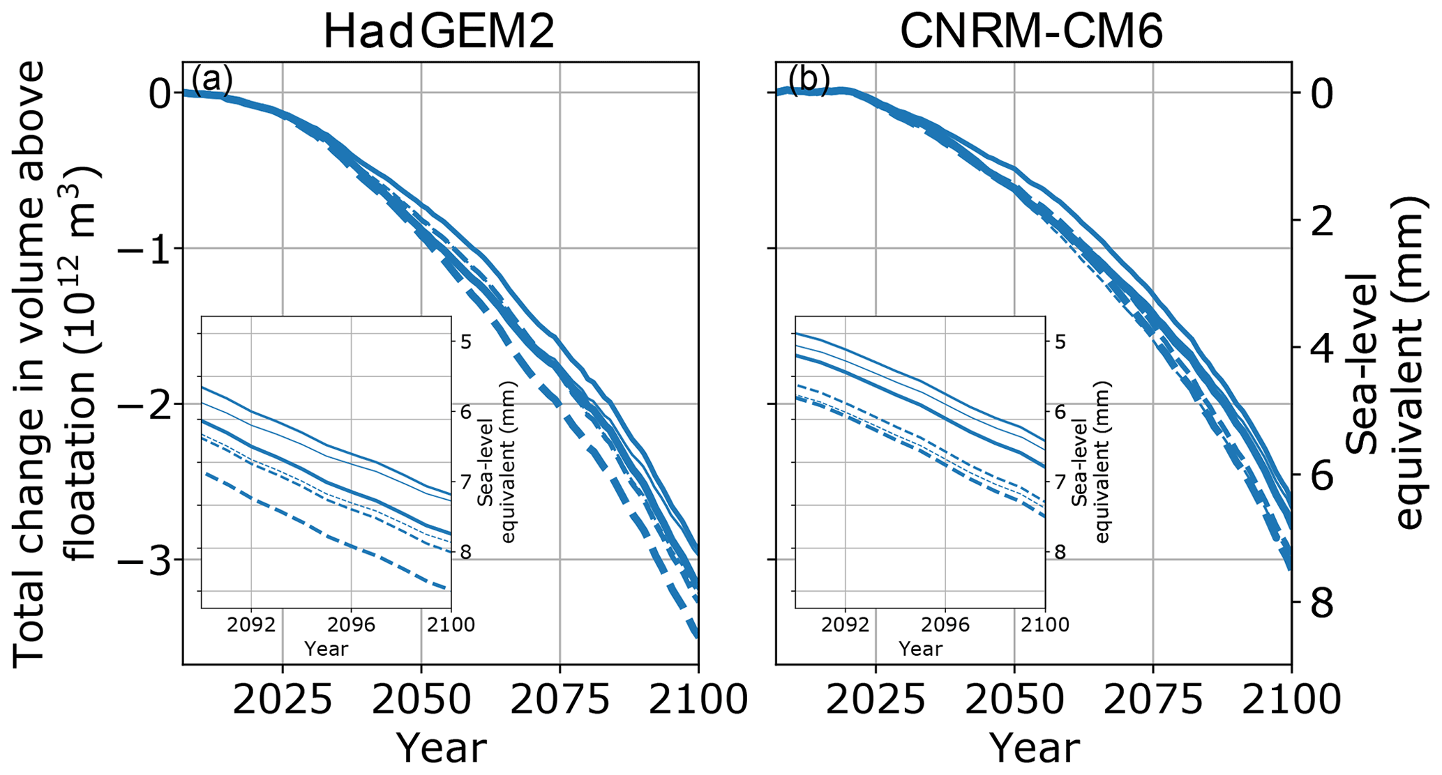
Figure 8Results of the ice-shelf melt sensitivity test. As in other figures, the solid and dashed curves represent and , respectively. Line thickness corresponds to sub-shelf melt rate tuning. Thin: 10 m yr−1; medium: 20 m yr−1; thick: 30 m yr−1. The 20 m yr−1 melt runs are the same as the corresponding curves in Fig. 5. Insets show the last 10 years of the simulation.
3.2.3 Calving rate limit
Figure 9 shows the results of our sensitivity experiment with five choices of upper limits on iceberg calving rate: 1, 3, 5, and 7 km yr−1, as well as one with no upper limit. We find that removing this upper limit leads to unreasonably high sustained glacier velocities of 35–40 km yr−1, and brief surges in this range occur even with the 7 km yr−1 calving rate limit. Thus, we consider ≤5 km yr−1 to be the reasonable range of upper limits on calving rates for Humboldt Glacier using the von Mises stress calving parameterization and our semi-plastic bed rheology. While our choice of a 3 km yr−1 calving rate limit results in a ∼ 15 % uncertainty in sea-level contribution in this case, this choice could combine non-linearly with choices of climate forcing, the calving scenario, and the basal friction law, leading to a larger overall uncertainty. We also note that the extent of the ice shelf is greatly reduced for assumed maximum calving rates of ≥5 km yr−1. Because a maximum calving rate of 5 km yr−1 still gives reasonable results, it is possible that the significant ice-shelf growth is a consequence of the assumed 3 km yr−1 maximum calving rate.
We have used the calving rate limit of 3 km yr−1 for the perturbed parameter ensemble because this limit was used in previous work (Choi et al., 2018) and because we are attempting to mitigate the positive feedback between calving rate and ice flow speed. It is not clear at what point this feedback becomes unphysical, even if modeled ice velocities remain within the range observed across the GrIS. However, we realize that our assumption may lead to a conservative estimate of SLR. To address this, we have run an additional set of three simulations using all three climate forcings, , low σmax, and a calving rate limit of 5 km yr−1 to estimate an upper bound on mass loss from Humboldt Glacier by 2100 (Fig. S10). We find an upper bound of ∼ 11–12 mm SLR, depending on climate forcing, compared with 7.8–8.7 mm using the 3 km yr−1 limit on calving.
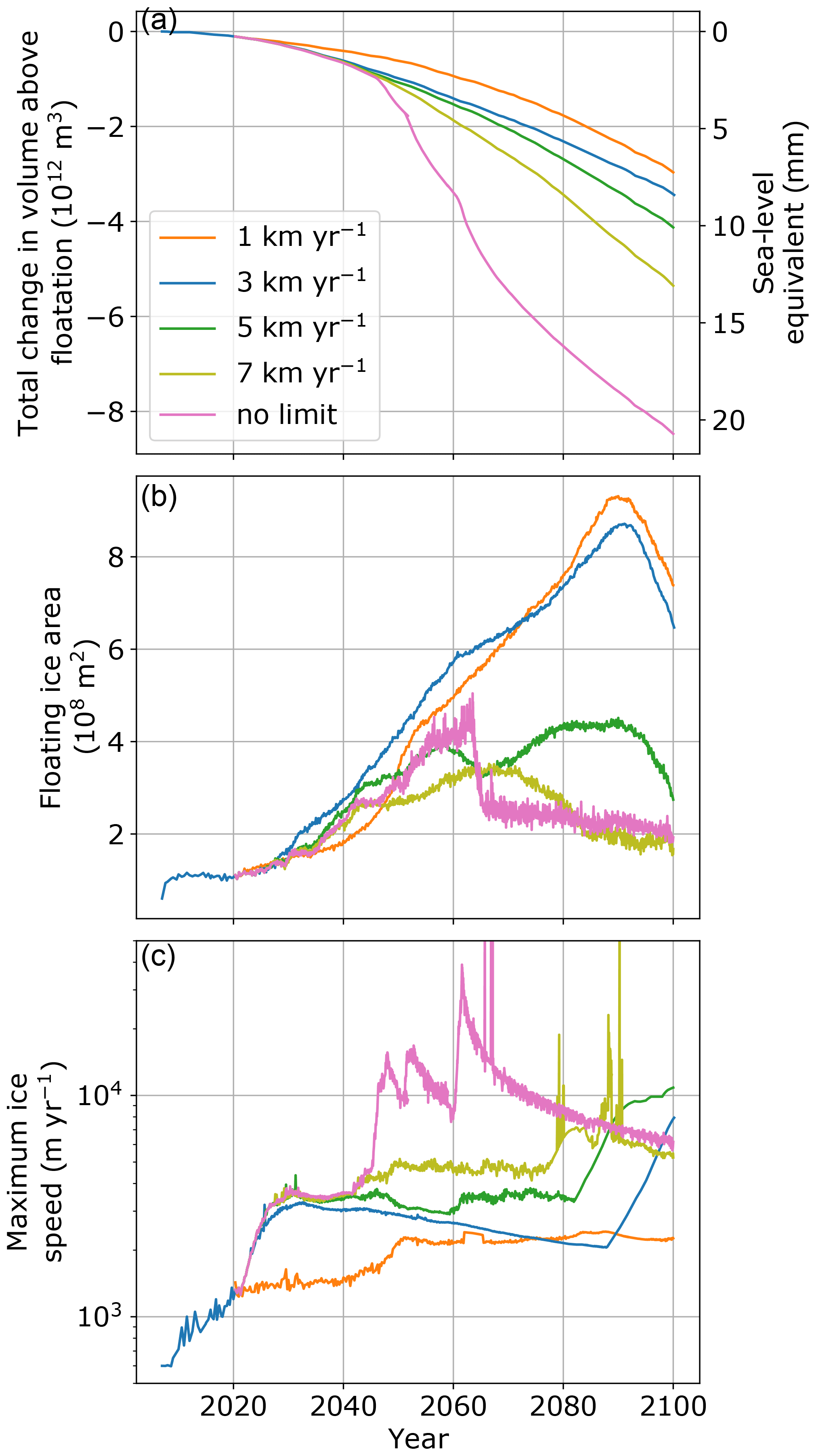
Figure 9Results of the calving rate limit sensitivity test. Line colors correspond to imposed calving rate limits. Based on the maximum modeled glacier speed in panel (c), we take ≤5 km yr−1 to be a reasonable range.
3.2.4 Bed topography
The new bathymetry data integrated into BedMachine version 4 result in significantly thicker ice at the glacier margin than in BedMachine version 3 (Rignot et al., 2021; Morlighem et al., 2017; Morlighem, 2017, 2021). We find that for the version 3 bed, the model requires a considerably more plastic basal friction law to match the observed speedup. We find exponents in the range of –, compared with – with the version 4 bed. Because of this more plastic bed rheology, our century-scale simulations with the version 3 bed predict a higher sea-level contribution by 2100 (Fig. 10). In general, the BMv3 simulations lose less mass early in the century, but all the BMv3 simulations surpass their BMv4 counterparts in terms of SLR contribution in the latter part of the century, due to increased ice flux allowed by the more plastic basal friction law. We also find that simulations using the BMv3 bed topography exhibit ice-shelf growth later in the century than in the corresponding BMv4 bed topography simulations.

Figure 10Results from the bed topography sensitivity test. Line colors correspond to the bed topography product version. As in other figures, the solid and dashed blue curves represent and , respectively; for pink, solid and dashed curves are and , respectively.
4.1 Controls on historical retreat of Humboldt Glacier
We find that melt undercutting at the grounded glacier terminus is a significant contributor to the predicted retreat over the observational period through its control on iceberg calving (Figs. 6, S9). However, the amount of submarine melt does not directly dominate the retreat as found by Rignot et al. (2021). This discrepancy could be due to the fact that we use model-based thermal forcing fields provided by ISMIP6 to calculate melt, rather than directly using CTD data. The existence of some floating ice in our simulations over the historical period also leads to basal melt rather than melting of the grounded terminus in these areas. We also do not take into account the “calving multiplier effect” by which melt undercutting drives higher calving rates even when it does not directly cause grounded ice to go afloat (O'Leary and Christofferson, 2013; Benn et al., 2017), which would depend on resolving the geometry of the face of the glacier terminus (Slater et al., 2021). This lack of an amplified influence of submarine melting on calving could be one reason for the small values of σmax necessary to initiate retreat. In other words, σmax may need to be small in the model to make up for the unresolved process of higher tensile stresses induced by undercutting.
We initialize and calibrate our model using winter velocities. We do not simulate the seasonal velocity cycles observed at Greenland outlet glaciers, which are often strongly controlled by surface runoff to the subglacial hydrologic system (Hoffman and Price, 2014; Moon et al., 2014) or by changes in buttressing due to melange and ice tongue formation and breakup (Joughin et al., 2012). The seasonal velocity cycle observed at Humboldt Glacier is strong, with velocities temporarily doubling or tripling near the terminus in summer compared with winter (Joughin et al., 2010, 2021). This seasonal cycle is superimposed on the longer-term tripling of velocity near the terminus and a 50 % increase in velocity ∼ 25 km upglacier of the terminus between 2012 and 2017 (Fig. 1; Joughin et al., 2018), during which time the terminus retreated 1–3 km in the north and <1 km in the south (Joughin et al., 2015, 2017; Moon and Joughin 2008). We attempt to reproduce this longer-term acceleration by tuning the basal friction law exponent and the von Mises threshold stress parameter. Reproducing the full seasonal cycle would likely require coupling our ice dynamics model to a subglacial hydrology model, which is currently a major challenge for ice sheet simulations (Flowers, 2018). The summer acceleration is accompanied by terminus retreat at other Greenland outlet glaciers, as higher extensional strain rates promote calving (Kehrl et al., 2017). Thus, we may also need to use the small value of σmax≤200 kPa because we do not reproduce the high summer velocities, strain rates, and tensile stresses that induce most calving in reality. If the seasonal cycle persists through the 21st century, our simulated mass loss could be an underestimate, as we do not capture the summer months during which flux through the glacier is much larger than the annual average. However, using mean annual velocities instead of winter velocities would impose a modeled glacier state that only represents reality for a very small fraction of the year, while using only summer velocities would greatly overestimate dynamic mass loss. Thus, using winter velocities for initialization and calibration provides not only a more conservative but also a more representative model compared with using mean annual or summer velocities in the absence of a modeled seasonal velocity cycle.
In a sensitivity analysis of a flowline model, Carr et al. (2015) found that the greater retreat of the northern section compared with the southern section of the Humboldt Glacier terminus could be partially due to sea-ice buttressing and meltwater depth in crevasses. They found that rising air temperatures (and thus presumably increased meltwater flux into crevasses) and a decrease in sea-ice concentration coincided with the initiation of its rapid retreat after 1999. We have not represented these processes in our model, yet we are able to reproduce the historical behavior relatively well. Because of the numerous differences between our model and theirs (bed topography, number of spatial dimensions, stress balance approximation, plasticity of the basal friction law, choice of calving parameterization, etc.), a direct comparison to their results is not feasible. However, we note that Carr et al. (2015) use a basal friction law exponent of , while we find necessary to match observed changes. They also do not include submarine melting in their model experiments, concluding that it is likely a small contribution. In broad agreement with the results of Rignot et al. (2021), we have found that submarine melt is in fact an important factor in the retreat of Humboldt Glacier (Figs. 6, S9). However, if meltwater in crevasses and sea-ice concentration are indeed primary controls on the past and present retreat of Humboldt Glacier, then it could become more sensitive to surface and ocean temperatures as the climate warms than we have accounted for here. Whether this increased sensitivity would lead to significantly more sea-level rise from Humboldt than we estimate here is an open question.
4.2 Comparison to previous 21st century projections from Greenland
Our estimated SLR contribution of 5.2–8.7 mm by 2100 is considerably higher than a recent estimate of ∼ 3.5 mm from Humboldt Glacier (Choi et al., 2021). We attribute this primarily to our calibration of the basal friction law to match observed surface velocity changes. Choi et al. (2021) used a linear-viscous treatment of basal friction and did not attempt to reproduce the speedup over the historical period. In their projection for Humboldt Glacier, the contribution from surface mass balance was about 50 % larger than the dynamic contribution by 2100. In our von Mises stress calving simulations, ice dynamics (including both ice flow and calving) is the larger direct contributor in most cases (Figs. 5, 6), although some of the ice dynamical response is also driven by surface mass balance. While our estimate differs from theirs, our findings support their conclusion that ice dynamics will continue to be an important part of the GrIS mass budget through the 21st century.
Our projected SLR contribution is also a sizable fraction of the 90 ± 50 mm SLR from the whole GrIS by 2100 predicted by the ISMIP6 multi-model ensemble for the RCP8.5 emissions scenario (Goelzer et al., 2020). There are too many degrees of freedom between the many models and modeling choices used in the ISMIP6 whole-GrIS ensemble to determine whether our basal friction law tuning is the reason for this, but we suspect that it is a primary contributor because our tuned basal friction law exponent leads to up to twice as much mass loss when compared with an assumed linear-viscous basal friction law (Fig. 5). However, because Humboldt Glacier represents ∼ 5 % of the area of the Greenland Ice sheet, our lower bound of 6.2 mm from the von Mises calving simulations represents a proportional contribution when compared with the upper value of 140 mm from ISMIP6 for the whole GrIS (Goelzer et al., 2020). If the behavior we find here extends to other major outlet glaciers (e.g., Åkesson et al., 2021), then the ISMIP6 projections from models using linear or Weertman basal friction relationships may systematically underestimate 21st century retreat and mass loss.
It is unclear whether the higher climate sensitivity of the CMIP6 models compared with CMIP5 represents an improvement in climate forecasting (Edwards et al., 2021; Payne et al., 2021). The single CMIP6 climate forcing we include here (CNRM-CM6) predicts high positive surface mass balance towards the glacier interior, resulting in a net positive surface mass balance contribution for the first half of our simulations, while the two CMIP5 climate forcings predict net negative surface mass balance contribution through the entire century (Fig. 6). However, the steeper negative slope of the CNRM-CM6 forcing by the end of the century indicates that the 22nd century could see extreme negative surface mass balance dominating mass loss (e.g., Goelzer et al., 2013). Other CMIP5 and CMIP6 earth system models and high-resolution regional climate modeling (not examined here) agree on a net negative surface mass balance for the GrIS after about 2055 (Noël et al., 2021). Thus, while we find a slightly larger direct SLR contribution from ice dynamics than from surface mass balance, these relative magnitudes could change after 2100. However, because surface mass balance influences ice dynamics through its various effects on basal friction (changing both ice overburden and basal water pressure in reality), these two contributions cannot be completely disentangled.
4.3 Influence of the basal friction law
Our choice of an effective pressure-dependent power-law (Budd-type) basal friction relationship was motivated by the need to match the observed tripling of flow speed at the northern section of the marine terminus in the observational period (Figs. 1, 3), for which a linear-viscous basal friction law is not suitable. However, the proper representation of the effective pressure term in this relationship is highly uncertain. As in many previous studies, we use the assumption that the subglacial hydrologic system is perfectly connected to the ocean (e.g., Vieli et al., 2001; Seroussi et al., 2013; Asay-Davis et al., 2016; Morlighem et al., 2019). However, this assumption can lead to effective pressures that increase too rapidly with distance from the grounding line when compared with output of a subglacial hydrology model (Smith-Johnsen et al., 2020; Hager et al., 2022). While this problem is offset by the basal friction parameter μ in the optimization, long-term projections are complicated by the resulting spatial pattern, which likely leads to values of μ that are inappropriately low when the grounding line has retreated far inland. We do not expect this to be a significant issue in our century-scale runs, as the grounding line only retreats ∼ 30 km in our most aggressive scenario (, HadGEM2 climate, low σmax) (Fig. 4), where μ is still relatively high and effective pressure in the initial condition is relatively low. In the absence of a subglacial hydrology model coupled to the ice dynamics model, better treatments of effective pressure are not readily available. However, simple parameterizations of effective pressure that produce the lower gradients observed in results of a subglacial hydrology model (e.g., Downs and Johnson, 2022) could improve the reliability of long-term projections.
While we have explored the parameter uncertainty within our chosen Budd-type basal friction relationship (Budd et al., 1979, 1984) by using a range of power-law exponents, we have not explored uncertainty in the basal friction coefficient, μ, from our optimization. Because μ is a spatially variable field, quantifying this uncertainty would require advanced and expensive approaches, such as Bayesian inference with Markov chain Monte Carlo sampling (see, e.g., Petra et al., 2014), which are beyond the scope of this study. The uncertainty in μ depends on uncertainties in the surface velocity data, the stress balance approximation and enthalpy model, uncertainty in the bed topography, and other model parameters. In reality, the rheology of the bed is also likely to vary spatially, which indicates that the basal friction law exponent, q, would ideally be a spatially varying field (De Rydt et al., 2021). Ideally, we could optimize q against observations as well as μ; however, the parameters q and μ are highly interdependent, and a snapshot optimization would not be able to differentiate the separate contribution of each field. Hence, a more advanced transient optimization would be required, which is beyond the scope of this study.
We have also not explored the structural uncertainty inherent in the choice of the form of the basal friction law. Other commonly used basal friction relationships include (1) a linear-viscous relationship with or without effective pressure dependence, (2) a power-law relationship (with q typically taken to be ) that is not dependent on effective pressure (Weertman, 1957), (3) a fully plastic till strength Coulomb law used for soft beds (Tulaczyk et al., 2000a, b), (4) a regularized Coulomb relationship in which the influence of effective pressure reduces with distance from the grounding line (Schoof, 2005; Joughin et al., 2019), and (5) a combined treatment with a sharp transition between Coulomb and power-law friction (Tsai et al., 2015). Of this list, our chosen semi-plastic Budd-type law and laws 3–5 above are appropriate for representing fast flow in ice sheets. The linear-viscous relationship is technically valid only for regelation-dominated basal flow, which is in general much slower than enhanced creep or sliding (Weertman, 1957; Fowler, 2010). The Weertman (1957) law is in general considered valid for hard beds with basal flow dominated by enhanced creep, while sliding beneath ice sheets is generally considered to be strongly dependent on till deformation and subglacial water pressure (e.g., Tulaczyk et al., 2000a, b; Zoet and Iverson, 2020). However, both the linear-viscous and Weertman laws are still widely used for ice-sheet-scale simulations, despite being largely inappropriate for representing fast ice flow. For example, 6 of the 15 models participating in the Antarctic Buttressing Model Intercomparison Project use a Weertman-style basal friction relationship, and another 3 use a linear-viscous relationship (Sun et al., 2020). The basal friction relationships used by the models participating in ISMIP6 Greenland are not systematically reported, but 6 of the 8 reported (out of 13 total) use a linear relationship or a power-law relationship with an exponent of (Goelzer et al., 2020). More widespread use of observed temporal speed changes to calibrate the basal friction relationship would likely lead modelers to abandon the Weertman and linear-viscous laws in large-scale ice sheet model simulations (e.g., Gillet-Chaulet et al., 2016; Joughin et al., 2019).
Our tuning of the basal friction law exponent underscores the point that optimizing the basal friction parameter can give a good fit to observations at the initial condition for most choices of the basal friction law but that thereafter the evolution diverges widely based on this choice (Gillet-Chaulet et al., 2016; Nias et al., 2018; Brondex et al., 2019; Joughin et al., 2019; Åkesson et al., 2021). Hindcasting simulations used to tune the basal friction law to reproduce observed changes are thus necessary to reduce uncertainty in projections of future behavior. However, there does not seem to be any consensus on the best form of the basal friction relationship, and the best choice could be glacier- or basin-dependent (Barnes and Gudmundsson, 2022). Additionally, the regularized Coulomb and fully plastic till strength relationships have additional unknown parameters that either need to be optimized by inverse methods, tuned in forward runs, or explored in sensitivity tests and which in reality would likely exhibit wide spatial variation.
The form of the basal friction relationship often exerts a strong control on modeled glacier behavior (Brondex et al., 2017, 2019; Nias et al., 2018; Joughin et al., 2019; Åkesson et al., 2021), but there seems to be no rule of thumb for determining a priori the relative magnitudes of mass loss between the Budd-type and regularized Coulomb basal friction laws. For instance, Brondex et al. (2019) found that Pine Island and Thwaites glaciers thinned and retreated less with the Budd law than with the Coulomb law, while Cosgrove and Dotson glaciers retreated considerably more with the Budd law than with the Coulomb law. Åkesson et al. (2021) also found that the Budd law led to greater mass loss than the regularized Coulomb law at Petermann Glacier, even though these two gave the best fits to observations of the laws they examined. Thus, it appears that the relative influence of these basal friction relationships on mass loss may be dependent on bed or ice geometry, and so we cannot confidently state whether using regularized Coulomb friction law would lead to more or less mass loss than we predict using the Budd-type law.
4.4 Influence of the iceberg calving law
We find that the von Mises stress calving law leads to a positive feedback between calving and ice velocity, which is exacerbated by our non-linear basal friction law (Fig. 9). The imposed upper bound of 3 km yr−1 on the calving rate is an ad hoc measure to prevent the runaway feedback between basal friction, ice velocity, and calving rate. While previous studies have used an upper bound on iceberg calving for this and other calving laws (e.g., DeConto and Pollard, 2016; Choi et al., 2018), this is a problem that should be rectified with improved calving parameterizations and calving fronts resolved in three dimensions, both of which pose significant challenges. The issues we find with the von Mises stress calving law lend some support to the suggestion that calving front position parameterizations should be used instead of calving rate parameterizations (Amaral et al., 2020). However, many existing calving front position parameterizations are without a convincing physical basis (for example, the calving laws based on height or thickness above floatation), while calving rate parameterizations like the von Mises stress formulation are desirable because they take the stress and strain rate fields into account. The crevasse depth model (Benn et al., 2007; Nick et al., 2010) generally recommended by Amaral et al. (2020) could be a good alternative to the von Mises calving law. However, Amaral et al. (2020) found that it performed worse than the von Mises stress calving law at Humboldt Glacier. It is also unclear how the crevasse water depth tuning parameter should evolve in time as surface melt increases. We have not used it here for these reasons, but we acknowledge that it could alleviate some of the problems we find with the von Mises calving law, which could potentially justify accepting a decreased ability to match observed retreat rates.
We use a single spatially uniform value of σmax in each simulation, as in previous work (Morlighem et al., 2016, 2019; Choi et al., 2018, 2021). Another option would be to use different values of σmax for grounded and floating ice (Choi et al., 2017), but because calving from the grounded margin is a relatively small contribution to the mass budget (Fig. 6), this is unlikely to have much impact on our results while greatly increasing the complexity of our calibration step. In reality σmax would likely be dependent on numerous factors such as ice fabric, temperature, damage, and meltwater availability for hydrofracture, all of which will vary in space and time. If σmax was allowed to evolve as some function of these properties, there could be potential for a negative feedback on calving as the calving front retreats into regions of stronger, less damaged ice or areas with less meltwater available. Whether this effect would be large enough to significantly impact our results is an open question.
Our simulations using the von Mises stress calving law require σmax≤200 kPa in order for Humboldt Glacier to retreat, while Amaral et al. (2020) found a σmax value of ∼ 2 MPa. We can identify a number of possible explanations for this discrepancy. First, Amaral et al. (2020) calibrated σmax along a 2 km wide flow band from 2012–2014, while we calculate the misfit across the full glacier terminus from winter 2007–2008 to winter 2017–2018, and we attempt to match both observed velocities and terminus positions. Second, our model does not reproduce the observed seasonal velocity cycle (Moon et al., 2014), while Amaral et al. (2020) used observations from May 2012 and June 2014, months on either side of the beginning of the summer speedup. For example, the velocity within 10 km of the terminus along the flow band analyzed by Amaral et al. (2020) doubled in the month between May and June 2014 (Joughin et al., 2021). This kind of seasonal acceleration is accompanied by terminus retreat at Helheim and Kangerlussuaq glaciers (Kehrl et al., 2017), and Humboldt could behave in a similar way. This could explain why observations that span the shoulder of the seasonal cycle (May and June) would require a higher σmax than is necessary for us to match mean observed retreat rates in our model: higher strain rates during seasonal acceleration result in a higher calculated von Mises stress, which in turn requires a higher value of σmax to match retreat. Finally, as noted above, we do not account for the calving multiplier effect, which could greatly increase tensile stresses behind undercut portions of the terminus. Given the considerable differences between our modeling and the observationally constrained approach of Amaral et al. (2020) – including different ice temperature fields, bed topography, resolutions, and time periods – we find this a sufficient reconciliation of the discrepancy in σmax. However, this illustrates that care should be taken when using values of tuning parameters from observational approaches directly in modeling studies, as the model may be missing physics or forcings that are implicitly accounted for in observations. As most ice sheet models do not reproduce the seasonal velocity cycle observed at Greenland outlet glaciers, the timing of observations used in model calibration and validation is of critical importance. Thus, we posit that σmax should be seen as a tuning parameter without much physical significance, and thus it may not fall within the reported range of ice tensile strength (e.g., Petrovic, 2003).
We have presented an ensemble of model simulations beginning from an optimized initial condition of Humboldt Glacier, northern Greenland, through the 21st century that are consistent with observed retreat rates and velocity changes from winter 2007–2008 to winter 2017–2018. We used three different climate forcings, spanning RCP8.5 and SSP5-8.5 scenarios from CMIP5 and CMIP6 models. Our main perturbed parameter ensemble explores the uncertainty in iceberg calving, climate forcing, and non-linearity of the basal sliding law, within the constraints provided by recent observations. In addition, we tested the sensitivity of the model to ice-shelf growth, sub-shelf melt rates, maximum calving rates, and bed topography.
The results of our perturbed parameter ensemble indicate that Humboldt Glacier is likely to contribute 6.2–8.7 mm to global mean sea level by 2100 under warm climate scenarios (RCP8.5 and SSP5-8.5), with variability due to the choice of the climate model, calving law tuning, and basal sliding law. Our minimum mass-loss estimates – which assume no additional retreat from calving after 2017 – range from 5.2–6.1 mm depending mainly on the choice of climate forcing. We find a relatively small range of acceptable tuning parameter values for the von Mises stress calving law (160–180 kPa or 170–190 kPa, depending on climate forcing and the basal friction law), but this leads to up to ∼ 1 mm variation in predicted sea-level rise contribution by 2100. These estimates are significantly higher than results from our own model using a linear basal friction law (4–5 mm), as well as another recent estimate using a different ice sheet model also with a linear basal friction law (∼ 3.5 mm; Choi et al., 2021). We note that a positive feedback between ice velocity and calving rates in the von Mises stress calving law results in considerable uncertainty in SLR estimates because an assumed maximum calving rate must be imposed. For reasonable assumptions of maximum calving rates (≤5 km yr−1 based on our sensitivity experiments), this could be as large as 30 %. Improved calving parameterizations are needed to reduce uncertainty in SLR estimates over timescales relevant to present-day policy decisions.
Our ensemble predicts the growth of a significant ice shelf by the middle of the 21st century in most simulations, which is still present by the end of the century for about two-thirds of cases. While this is not generally anticipated for Greenland outlet glaciers, it is a robust feature of the model given that it occurs across many parameter combinations, although it is sensitive to the assumed maximum calving rate. In sensitivity experiments with the ice shelf removed in 2055, Humboldt Glacier contributed up to 2 mm more SLR by 2100, a maximum increase of ∼ 25 %. We also find that our projected SLR estimates are relatively insensitive to our choice of sub-shelf melt tuning.
Finally, we find that mass-loss projections are strongly dependent on the bed topography data product used in simulations. Using BedMachine v3 bed topography instead of that of v4 yields up to an additional 2 mm SLR by 2100 for the cases we examined, a maximum increase of 25 %. This is because the shallower bed in BedMachine v3 requires a much more plastic basal friction law (exponents of – for v3, compared to – for v4) to match observed velocity changes. Thus, uncertainty in the ice thickness near the Humboldt Glacier terminus – and potentially at many other GrIS outlet glaciers – could be a large source of uncertainty in estimates of future SLR. This indicates that forthcoming attempts to estimate the future SLR contribution from the GrIS should explore the propagation of the uncertainty in bed topography and ice thickness.
Our findings suggest a number of other ways to improve confidence in SLR projections from ice sheet models. Systematic calibration of basal friction and iceberg calving parameterizations to historical observations of both velocity and ice extent changes are necessary. For models of the whole GrIS, this may have to be done by individual basin or sector, rather than using a single parameterization for the whole ice sheet. Calibrating the basal friction relationship to observed speed changes will likely lead to the abandonment of the commonly used linear-viscous and Weertman basal friction relationships in favor of more physically based parameterizations, which could lead to substantially higher estimates of SLR by 2100. Thus, current estimates of SLR from the GrIS this century could be substantially too conservative due to the numerous and significant challenges involved in calibrating models of the whole ice sheet. Parameterizations of iceberg calving continue to improve, but they are still a primary source of uncertainty. Finally, improved parameterizations of effective pressure are likely necessary for longer-term projections involving significant grounding-line retreat.
In summary, we find that Humboldt Glacier is likely to make a significant contribution to SLR this century and that, to date, its potential contribution has been underestimated. While the precision of our estimate is limited by the current state of understanding of iceberg calving, basal sliding, bed topography, and the magnitudes of future warming of the ocean and atmosphere, all of our model simulations predict continued retreat of Humboldt Glacier that will lead to the deglaciation of the majority of its deep marine-based area by 2100. Our findings indicate that ice dynamics, rather than surface mass balance, could be the dominant term in the mass budget of Humboldt Glacier this century.
Model input, output, code, and analysis scripts are publicly archived and available online at https://doi.org/10.5281/zenodo.5914667 (Hillebrand et al., 2022). The archive contains annual two- and three-dimensional model output that can be visualized using ParaView (https://www.paraview.org, last access: 27 October 2022). Scalar outputs are available for every time step. Two- and three-dimensional model output for each time step can be made available upon request but is not necessary to reproduce the analysis or figures. The versions of the MALI and Albany code used in this study can also be found on GitHub at https://github.com/MALI-Dev/E3SM/tree/d0c286778a6a035c600af891a268ed9f843aac52 (last access: 31 October 2022) and https://github.com/sandialabs/Albany/tree/ecbc0182015fda8d6a2bb29eaa3a47c260f40b13 (last access: 31 October 2022).
The supplement related to this article is available online at: https://doi.org/10.5194/tc-16-4679-2022-supplement.
IMH, SFP, TRH, and MJH conceived the study. TRH and MJH designed the model experiments. TRH implemented calving and melting parameterizations in the model code, performed the model simulations and analysis, and wrote the manuscript with input from all authors. MJH, TRH, SFP, and MP developed the ice sheet model. MP performed the optimization for the initial condition. IMH provided expertise in the use of remote sensing data.
The contact author has declared that none of the authors has any competing interests.
Sandia National Laboratories is a multimission laboratory managed and operated by National Technology and Engineering Solutions of Sandia, LLC., a wholly owned subsidiary of Honeywell International, Inc., for the U.S. Department of Energy’s National Nuclear Security Administration (contract no. DE-NA-0003525).
This paper describes objective technical results and analysis. Any subjective views or opinions that might be expressed in the paper do not necessarily represent the views of the U.S. Department of Energy or the United States Government.
Publisher’s note: Copernicus Publications remains neutral with regard to jurisdictional claims in published maps and institutional affiliations.
Simulations were performed on machines at the National Energy Research Scientific Computing Center (NERSC), a U.S. Department of Energy Office of Science User Facility located at Lawrence Berkeley National Laboratory (contract no. DE-AC02-05CH11231; NERSC award no. ERCAP0016816). We also used computing resources of the Los Alamos National Laboratory Institutional Computing Program, which is supported by the U.S. Department of Energy National Nuclear Security Administration (contract no. DE-AC52-06NA25396). We thank Michael Kelleher for assistance with data processing. We thank Johannes J. Fürst and two anonymous reviewers for comments that have greatly improved the paper.
This research has been supported by the Biological and Environmental Research program (Energy Exascale Earth System Model, E3SM; Scientific Discovery through Advanced Computing; Probabilistic Sea Level Projections from Ice Sheet and Earth System Models) and the Advanced Scientific Computing Research program (Scientific Discovery through Advanced Computing program; Probabilistic Sea Level Projections from Ice Sheet and Earth System Models), both within the U.S. Department of Energy Office of Science, and by the National Aeronautics and Space Administration (grant nos. 80NSSC18K1027 and NNX13AI21A).
This paper was edited by Johannes J. Fürst and reviewed by two anonymous referees.
Åkesson, H., Morlighem, M., O'Regan, M., and Jakobsson, M.: Future Projections of Petermann Glacier Under Ocean Warming Depend Strongly on Friction Law, J. Geophys. Res.-Earth, 126, e2020JF005921, https://doi.org/10.1029/2020JF005921, 2021.
Albrecht, T., Martin, M., Haseloff, M., Winkelmann, R., and Levermann, A.: Parameterization for subgrid-scale motion of ice-shelf calving fronts, The Cryosphere, 5, 35–44, https://doi.org/10.5194/tc-5-35-2011, 2011.
Amaral, T., Bartholomaus, T. C., and Enderlin, E. M.: Evaluation of Iceberg Calving Models Against Observations From Greenland Outlet Glaciers, J. Geophys. Res.-Earth, 125, e2019JF005444, https://doi.org/10.1029/2019JF005444, 2020.
Asay-Davis, X. S., Cornford, S. L., Durand, G., Galton-Fenzi, B. K., Gladstone, R. M., Gudmundsson, G. H., Hattermann, T., Holland, D. M., Holland, D., Holland, P. R., Martin, D. F., Mathiot, P., Pattyn, F., and Seroussi, H.: Experimental design for three interrelated marine ice sheet and ocean model intercomparison projects: MISMIP v. 3 (MISMIP +), ISOMIP v. 2 (ISOMIP +) and MISOMIP v. 1 (MISOMIP1), Geosci. Model Dev., 9, 2471–2497, https://doi.org/10.5194/gmd-9-2471-2016, 2016.
Aschwanden, A., Bueler, E., Khroulev, C., and Blatter, H.: An enthalpy formulation for glaciers and ice sheets, J. Glaciol., 58, 441–457, https://doi.org/10.3189/2012JoG11J088, 2012.
Banwell, A. F., MacAyeal, D. R., and Sergienko, O. V.: Breakup of the Larsen B Ice Shelf triggered by chain reaction drainage of supraglacial lakes, Geophys. Res. Lett., 40, 5872–5876, https://doi.org/10.1002/2013GL057694, 2013.
Barnes, J. M. and Gudmundsson, G. H.: The predictive power of ice sheet models and the regional sensitivity of ice loss to basal sliding parameterisations: a case study of Pine Island and Thwaites glaciers, West Antarctica, The Cryosphere, 16, 4291–4304, https://doi.org/10.5194/tc-16-4291-2022, 2022.
Barthel, A., Agosta, C., Little, C. M., Hattermann, T., Jourdain, N. C., Goelzer, H., Nowicki, S., Seroussi, H., Straneo, F., and Bracegirdle, T. J.: CMIP5 model selection for ISMIP6 ice sheet model forcing: Greenland and Antarctica, The Cryosphere, 14, 855–879, https://doi.org/10.5194/tc-14-855-2020, 2020.
Benn, D. I., Warren, C. R., and Mottram, R. H.: Calving processes and the dynamics of calving glaciers, Earth-Sci. Rev., 82, 143–179, https://doi.org/10.1016/j.earscirev.2007.02.002, 2007.
Benn, D. I., Åström, J., Zwinger, T., Todd, J., Nick, F. M., Cook, S., Hulton, N. R. J., and Luckman, A.: Melt-under-cutting and buoyancy-driven calving from tidewater glaciers: new insights from discrete element and continuum model simulations, J. Glaciol., 63, 691–702, https://doi.org/10.1017/jog.2017.41, 2017.
Blatter, H.: Velocity and stress fields in grounded glaciers: a simple algorithm for including deviatoric stress gradients, J. Glaciol., 41, 333–344, https://doi.org/10.3189/S002214300001621X, 1995.
Box, J. E. and Decker, D. T.: Greenland marine-terminating glacier area changes: 2000–2010, Ann. Glaciol., 52, 91–98, https://doi.org/10.3189/172756411799096312, 2011.
Brondex, J., Gagliardini, O., Gillet-Chaulet, F., and Durand, G.: Sensitivity of grounding line dynamics to the choice of the friction law, J. Glaciol., 63, 854–866, https://doi.org/10.1017/jog.2017.51, 2017.
Brondex, J., Gillet-Chaulet, F., and Gagliardini, O.: Sensitivity of centennial mass loss projections of the Amundsen basin to the friction law, The Cryosphere, 13, 177–195, https://doi.org/10.5194/tc-13-177-2019, 2019.
Budd, W. F., Keage, P. L., and Blundy, N. A.: Empirical Studies of Ice Sliding, J. Glaciol., 23, 157–170, https://doi.org/10.3189/S0022143000029804, 1979.
Budd, W. F., Jenssen, D., and Smith, I. N.: A Three-Dimensional Time-Dependent Model of the West Antarctic Ice Sheet, Ann. Glaciol., 5, 29–36, https://doi.org/10.3189/1984AoG5-1-29-36, 1984.
Cai, C., Rignot, E., Menemenlis, D., and Nakayama, Y.: Observations and modeling of ocean-induced melt beneath Petermann Glacier Ice Shelf in northwestern Greenland, Geophys. Res. Lett., 44, 8396–8403, https://doi.org/10.1002/2017GL073711, 2017.
Carr, J. R., Vieli, A., Stokes, C. R., Jamieson, S. S. R., Palmer, S. J., Christoffersen, P., Dowdeswell, J. A., Nick, F. M., Blankenship, D. D., and Young, D. A.: Basal topographic controls on rapid retreat of Humboldt Glacier, northern Greenland, J. Glaciol., 61, 137–150, https://doi.org/10.3189/2015JoG14J128, 2015.
Choi, Y., Morlighem, M., Rignot, E., Mouginot, J., and Wood, M.: Modeling the Response of Nioghalvfjerdsfjorden and Zachariae Isstrøm Glaciers, Greenland, to Ocean Forcing Over the Next Century, Geophys. Res. Lett., 44, 11071–11079, https://doi.org/10.1002/2017GL075174, 2017.
Choi, Y., Morlighem, M., Wood, M., and Bondzio, J. H.: Comparison of four calving laws to model Greenland outlet glaciers, The Cryosphere, 12, 3735–3746, https://doi.org/10.5194/tc-12-3735-2018, 2018.
Choi, Y., Morlighem, M., Rignot, E., and Wood, M.: Ice dynamics will remain a primary driver of Greenland ice sheet mass loss over the next century, Communications Earth & Environment, 2, 26, https://doi.org/10.1038/s43247-021-00092-z, 2021.
DeConto, R. M. and Pollard, D.: Contribution of Antarctica to past and future sea-level rise, Nature, 531, 591–597, https://doi.org/10.1038/nature17145, 2016.
De Rydt, J., Reese, R., Paolo, F. S., and Gudmundsson, G. H.: Drivers of Pine Island Glacier speed-up between 1996 and 2016, The Cryosphere, 15, 113–132, https://doi.org/10.5194/tc-15-113-2021, 2021.
Downs, J. and Johnson, J. V.: A rapidly retreating, marine-terminating glacier's modeled response to perturbations in basal traction, J. Glaciol., 68, 891–900, https://doi.org/10.1017/jog.2022.5, 2022.
Edwards, T. L., Nowicki, S., Marzeion, B., Hock, R., Goelzer, H., Seroussi, H., Jourdain, N. C., Slater, D. A., Turner, F. E., Smith, C. J., McKenna, C. M., Simon, E., Abe-Ouchi, A., Gregory, J. M., Larour, E., Lipscomb, W. H., Payne, A. J., Shepherd, A., Agosta, C., Alexander, P., Albrecht, T., Anderson, B., Asay-Davis, X., Aschwanden, A., Barthel, A., Bliss, A., Calov, R., Chambers, C., Champollion, N., Choi, Y., Cullather, R., Cuzzone, J., Dumas, C., Felikson, D., Fettweis, X., Fujita, K., Galton-Fenzi, B. K., Gladstone, R., Golledge, N. R., Greve, R., Hattermann, T., Hoffman, M. J., Humbert, A., Huss, M., Huybrechts, P., Immerzeel, W., Kleiner, T., Kraaijenbrink, P., Le Clec'h, S., Lee, V., Leguy, G. R., Little, C. M., Lowry, D. P., Malles, J.-H., Martin, D. F., Maussion, F., Morlighem, M., O'Neill, J. F., Nias, I., Pattyn, F., Pelle, T., Price, S. F., Quiquet, A., Radić, V., Reese, R., Rounce, D. R., Rückamp, M., Sakai, A., Shafer, C., Schlegel, N.-J., Shannon, S., Smith, R. S., Straneo, F., Sun, S., Tarasov, L., Trusel, L. D., Van Breedam, J., van de Wal, R., van den Broeke, M., Winkelmann, R., Zekollari, H., Zhao, C., Zhang, T., and Zwinger, T.: Projected land ice contributions to twenty-first-century sea level rise, Nature, 593, 74–82, https://doi.org/10.1038/s41586-021-03302-y, 2021.
Flowers, G. E.: Hydrology and the future of the Greenland Ice Sheet, Nat. Commun., 9, 2729, https://doi.org/10.1038/s41467-018-05002-0, 2018.
Fowler, A. C.: Weertman, Lliboutry and the development of sliding theory, J. Glaciol., 56, 965–972, https://doi.org/10.3189/002214311796406112, 2010.
Gillet-Chaulet, F., Durand, G., Gagliardini, O., Mosbeux, C., Mouginot, J., Rémy, F., and Ritz, C.: Assimilation of surface velocities acquired between 1996 and 2010 to constrain the form of the basal friction law under Pine Island Glacier, Geophys. Res. Lett., 43, 10311–10321, https://doi.org/10.1002/2016GL069937, 2016.
Glen, J. W.: The creep of polycrystalline ice, P. Roy. Soc. Lond. A: Mat., 228, 519–538, https://doi.org/10.1098/rspa.1955.0066, 1955.
Goelzer, H., Huybrechts, P., Fürst, J. J., Nick, F. M., Andersen, M. L., Edwards, T. L., Fettweis, X., Payne, A. J., and Shannon, S.: Sensitivity of Greenland Ice Sheet Projections to Model Formulations, J. Glaciol., 59, 733–749, https://doi.org/10.3189/2013JoG12J182, 2013.
Goelzer, H., Nowicki, S., Payne, A., Larour, E., Seroussi, H., Lipscomb, W. H., Gregory, J., Abe-Ouchi, A., Shepherd, A., Simon, E., Agosta, C., Alexander, P., Aschwanden, A., Barthel, A., Calov, R., Chambers, C., Choi, Y., Cuzzone, J., Dumas, C., Edwards, T., Felikson, D., Fettweis, X., Golledge, N. R., Greve, R., Humbert, A., Huybrechts, P., Le clec'h, S., Lee, V., Leguy, G., Little, C., Lowry, D. P., Morlighem, M., Nias, I., Quiquet, A., Rückamp, M., Schlegel, N.-J., Slater, D. A., Smith, R. S., Straneo, F., Tarasov, L., van de Wal, R., and van den Broeke, M.: The future sea-level contribution of the Greenland ice sheet: a multi-model ensemble study of ISMIP6, The Cryosphere, 14, 3071–3096, https://doi.org/10.5194/tc-14-3071-2020, 2020.
Hager, A. O., Hoffman, M. J., Price, S. F., and Schroeder, D. M.: Persistent, extensive channelized drainage modeled beneath Thwaites Glacier, West Antarctica, The Cryosphere, 16, 3575–3599, https://doi.org/10.5194/tc-16-3575-2022, 2022.
Hill, E. A., Carr, J. R., Stokes, C. R., and Gudmundsson, G. H.: Dynamic changes in outlet glaciers in northern Greenland from 1948 to 2015, The Cryosphere, 12, 3243–3263, https://doi.org/10.5194/tc-12-3243-2018, 2018.
Hillebrand, T. R., Hoffman, M. J., Perego, M., and Price, S. F.: MPAS-Albany Land Ice model simulations of Humboldt Glacier, North Greenland, from 2007–2100, Zenodo [code and data set], https://doi.org/10.5281/zenodo.5914667, 2022.
Hoffman, M. and Price, S.: Feedbacks between coupled subglacial hydrology and glacier dynamics, J. Geophys. Res.-Earth, 119, 414–436, 2014.
Hoffman, M. J., Perego, M., Price, S. F., Lipscomb, W. H., Zhang, T., Jacobsen, D., Tezaur, I., Salinger, A. G., Tuminaro, R., and Bertagna, L.: MPAS-Albany Land Ice (MALI): a variable-resolution ice sheet model for Earth system modeling using Voronoi grids, Geosci. Model Dev., 11, 3747–3780, https://doi.org/10.5194/gmd-11-3747-2018, 2018.
Holland, P. R., Jenkins, A., and Holland, D. M.: The Response of Ice Shelf Basal Melting to Variations in Ocean Temperature, J. Climate, 21, 2558–2572, https://doi.org/10.1175/2007JCLI1909.1, 2008.
Howat, I. M., Negrete, A., and Smith, B. E.: The Greenland Ice Mapping Project (GIMP) land classification and surface elevation data sets, The Cryosphere, 8, 1509–1518, https://doi.org/10.5194/tc-8-1509-2014, 2014.
Howat, I.: MEaSUREs Greenland Ice Mapping Project (GIMP) 2000 Image Mosaic, Version 1, NASA National Snow and Ice Data Center Distributed Active Archive Center, Boulder, Colorado USA [data set], https://doi.org/10.5067/4RNTRRE4JCYD 2017.
The IMBIE team: Mass balance of the Greenland Ice Sheet from 1992 to 2018, Nature, 579, 233–239, https://doi.org/10.1038/s41586-019-1855-2, 2019.
Jenkins, A.: A one-dimensional model of ice shelf-ocean interaction, J. Geophys. Res.-Oceans, 96, 20671–20677, https://doi.org/10.1029/91JC01842, 1991.
Joughin, I., Smith, B. E., Howat, I. M., Scambos, T., and Moon, T.: Greenland flow variability from ice-sheet-wide velocity mapping, J. Glaciol., 56, 415–430, https://doi.org/10.3189/002214310792447734, 2010.
Joughin, I., Smith, B. E., Howat, I. M., Floricioiu, D., Alley, R. B., Truffer, M., and Fahnestock, M.: Seasonal to decadal scale variations in the surface velocity of Jakobshavn Isbrae, Greenland: Observation and model-based analysis, J. Geophys. Res.-Earth, 117, F02030, https://doi.org/10.1029/2011JF002110, 2012.
Joughin, I., Smith, B., Howat, I., and Scambos, T.: MEaSUREs Greenland Ice Sheet Velocity Map from InSAR Data, Version 2, NASA National Snow and Ice Data Center Distributed Active Archive Center, Boulder, Colorado USA [data set], https://doi.org/10.5067/OC7B04ZM9G6Q, 2015.
Joughin, I., B. Smith, I. Howat, and T. Scambos: MEaSUREs Multi-year Greenland Ice Sheet Velocity Mosaic, Version 1, NASA National Snow and Ice Data Center Distributed Active Archive Center, Boulder, Colorado USA [data set], https://doi.org/10.5067/QUA5Q9SVMSJG, 2016.
Joughin, I., Moon, T., Joughin, J., and Black, T.: MEaSUREs Annual Greenland Outlet Glacier Terminus Positions from SAR Mosaics, Version 1, NASA National Snow and Ice Data Center Distributed Active Archive Center, Boulder, Colorado USA [data set], https://doi.org/10.5067/DC0MLBOCL3EL, 2017.
Joughin, I., Smith, B. E., and Howat, I. M.: A complete map of Greenland ice velocity derived from satellite data collected over 20 years, J. Glaciol., 64, 1–11, https://doi.org/10.1017/jog.2017.73, 2018.
Joughin, I., Smith, B. E., and Schoof, C. G.: Regularized Coulomb Friction Laws for Ice Sheet Sliding: Application to Pine Island Glacier, Antarctica, Geophys. Res. Lett., 46, 4764–4771, https://doi.org/10.1029/2019GL082526, 2019.
Joughin, I., Howat, I., Smith, B., and Scambos, T.: MEaSUREs Greenland Ice Velocity: Selected Glacier Site Velocity Maps from InSAR, Version 4, NASA National Snow and Ice Data Center Distributed Active Archive Center, Boulder, Colorado USA [data set], https://doi.org/10.5067/GQZQY2M5507Z, 2021.
Jourdain, N. C., Asay-Davis, X., Hattermann, T., Straneo, F., Seroussi, H., Little, C. M., and Nowicki, S.: A protocol for calculating basal melt rates in the ISMIP6 Antarctic ice sheet projections, The Cryosphere, 14, 3111–3134, https://doi.org/10.5194/tc-14-3111-2020, 2020.
Kehrl, L. M., Joughin, I., Shean, D. E., Floricioiu, D., and Krieger, L.: Seasonal and interannual variabilities in terminus position, glacier velocity, and surface elevation at Helheim and Kangerlussuaq Glaciers from 2008 to 2016, J. Geophys. Res.-Earth, 122, 1635–1652, https://doi.org/10.1002/2016JF004133, 2017.
King, M. D., Howat, I. M., Candela, S. G., Noh, M. J., Jeong, S., Noël, B. P., van den Broeke, M. R., Wouters, B., and Negrete, A.: Dynamic ice loss from the Greenland Ice Sheet driven by sustained glacier retreat, Commun. Earth Environ., 1, 1, https://doi.org/10.1038/s43247-020-0001-2, 2020.
Moon, T. and Joughin, I.: Changes in ice front position on Greenland's outlet glaciers from 1992 to 2007, J. Geophys. Res.-Earth, 113, F02022, https://doi.org/10.1029/2007JF000927, 2008.
Moon, T., Joughin, I., Smith, B., van den Broeke, M. R., van de Berg, W. J., Noël, B., and Usher, M.: Distinct patterns of seasonal Greenland glacier velocity, Geophys. Res. Lett., 41, 7209–7216, https://doi.org/10.1002/2014GL061836, 2014.
Morlighem, M.: IceBridge BedMachine Greenland, Version 3, NASA National Snow and Ice Data Center Distributed Active Archive Center, Boulder, Colorado USA [data set], https://doi.org/10.5067/2CIX82HUV88Y, 2017.
Morlighem, M., Bondzio, J., Seroussi, H., Rignot, E., Larour, E., Humbert, A., and Rebuffi, S.: Modeling of Store Gletscher's calving dynamics, West Greenland, in response to ocean thermal forcing, Geophys. Res. Lett., 43, 2659–2666, https://doi.org/10.1002/2016GL067695, 2016.
Morlighem, M., Williams, C. N., Rignot, E., An, L., Arndt, J. E., Bamber, J. L., Catania, G., Chauché, N., Dowdeswell, J. A., Dorschel, B., Fenty, I., Hogan, K., Howat, I., Hubbard, A., Jakobsson, M., Jordan, T. M., Kjeldsen, K. K., Millan, R., Mayer, L., Mouginot, J., Noël, B. P. Y., O'Cofaigh, C., Palmer, S., Rysgaard, S., Seroussi, H., Siegert, M. J., Slabon, P., Straneo, F., van den Broeke, M. R., Weinrebe, W., Wood, M., and Zinglersen, K. B.: BedMachine v3: Complete Bed Topography and Ocean Bathymetry Mapping of Greenland From Multibeam Echo Sounding Combined With Mass Conservation, Geophys. Res. Lett., 44, 11051–11061, https://doi.org/10.1002/2017GL074954, 2017.
Morlighem, M., Wood, M., Seroussi, H., Choi, Y., and Rignot, E.: Modeling the response of northwest Greenland to enhanced ocean thermal forcing and subglacial discharge, The Cryosphere, 13, 723–734, https://doi.org/10.5194/tc-13-723-2019, 2019.
Morlighem, M.: IceBridge BedMachine Greenland, Version 4, NASA National Snow and Ice Data Center Distributed Active Archive Center, Boulder, Colorado USA [data set], https://doi.org/10.5067/VLJ5YXKCNGXO, 2021.
Mottram, R., B. Simonsen, S., Høyer Svendsen, S., Barletta, V. R., Sandberg Sørensen, L., Nagler, T., Wuite, J., Groh, A., Horwath, M., Rosier, J., Solgaard, A., Hvidberg, C. S., and Forsberg, R.: An Integrated View of Greenland Ice Sheet Mass Changes Based on Models and Satellite Observations, Remote Sensing, 11, 1407, https://doi.org/10.3390/rs11121407, 2019.
Nias, I. J., Cornford, S. L., and Payne, A. J.: New Mass-Conserving Bedrock Topography for Pine Island Glacier Impacts Simulated Decadal Rates of Mass Loss, Geophys. Res. Lett., 45, 3173–3181, https://doi.org/10.1002/2017GL076493, 2018.
Nick, F. M., Veen, C. J. V. D., Vieli, A., and Benn, D. I.: A physically based calving model applied to marine outlet glaciers and implications for the glacier dynamics, J. Glaciol., 56, 781–794, https://doi.org/10.3189/002214310794457344, 2010.
Noël, B., van Kampenhout, L., Lenaerts, J. T. M., van de Berg, W. J., and van den Broeke, M. R.: A 21st Century Warming Threshold for Sustained Greenland Ice Sheet Mass Loss, Geophys. Res. Lett., 48, e2020GL090471, https://doi.org/10.1029/2020GL090471, 2021.
Nowicki, S., Goelzer, H., Seroussi, H., Payne, A. J., Lipscomb, W. H., Abe-Ouchi, A., Agosta, C., Alexander, P., Asay-Davis, X. S., Barthel, A., Bracegirdle, T. J., Cullather, R., Felikson, D., Fettweis, X., Gregory, J. M., Hattermann, T., Jourdain, N. C., Kuipers Munneke, P., Larour, E., Little, C. M., Morlighem, M., Nias, I., Shepherd, A., Simon, E., Slater, D., Smith, R. S., Straneo, F., Trusel, L. D., van den Broeke, M. R., and van de Wal, R.: Experimental protocol for sea level projections from ISMIP6 stand-alone ice sheet models, The Cryosphere, 14, 2331–2368, https://doi.org/10.5194/tc-14-2331-2020, 2020.
Nye, J. F.: The distribution of stress and velocity in glaciers and ice-sheets, P. Roy. Soc. Lond. A Mat., 239, 113–133, https://doi.org/10.1098/rspa.1957.0026, 1957.
O'Leary, M. and Christoffersen, P.: Calving on tidewater glaciers amplified by submarine frontal melting, The Cryosphere, 7, 119–128, https://doi.org/10.5194/tc-7-119-2013, 2013.
OMG: OMG Airborne eXpendable Conductivity Temperature Depth (AXCTD) Profiles, Ver. 1, PO. DAAC, CA, USA [data set], https://doi.org/10.5067/OMGEV-AXCT1, 2019.
OMG: OMG Conductivity, Temperature and Depth (CTD) profiles, Ver. 1, PO. DAAC, CA, USA [data set], https://doi.org/10.5067/OMGEV-CTDS1, 2020.
Pattyn, F.: A new three-dimensional higher-order thermomechanical ice sheet model: Basic sensitivity, ice stream development, and ice flow across subglacial lakes, J. Geophys. Res.-Sol. Ea., 108, 2382, https://doi.org/10.1029/2002JB002329, 2003.
Payne, A. J., Nowicki, S., Abe-Ouchi, A., Agosta, C., Alexander, P., Albrecht, T., Asay-Davis, X., Aschwanden, A., Barthel, A., Bracegirdle, T. J., Calov, R., Chambers, C., Choi, Y., Cullather, R., Cuzzone, J., Dumas, C., Edwards, T. L., Felikson, D., Fettweis, X., Galton-Fenzi, B. K., Goelzer, H., Gladstone, R., Golledge, N. R., Gregory, J. M., Greve, R., Hattermann, T., Hoffman, M. J., Humbert, A., Huybrechts, P., Jourdain, N. C., Kleiner, T., Munneke, P. K., Larour, E., Clec'h, S. L., Lee, V., Leguy, G., Lipscomb, W. H., Little, C. M., Lowry, D. P., Morlighem, M., Nias, I., Pattyn, F., Pelle, T., Price, S. F., Quiquet, A., Reese, R., Rückamp, M., Schlegel, N.-J., Seroussi, H., Shepherd, A., Simon, E., Slater, D., Smith, R. S., Straneo, F., Sun, S., Tarasov, L., Trusel, L. D., Breedam, J. V., Wal, R. van de, Broeke, M. van den, Winkelmann, R., Zhao, C., Zhang, T., and Zwinger, T.: Future Sea Level Change Under Coupled Model Intercomparison Project Phase 5 and Phase 6 Scenarios From the Greenland and Antarctic Ice Sheets, Geophys. Res. Lett., 48, e2020GL091741, https://doi.org/10.1029/2020GL091741, 2021.
Perego, M., Price, S., and Stadler, G.: Optimal initial conditions for coupling ice sheet models to Earth system models, J. Geophys. Res.-Earth, 119, 1894–1917, https://doi.org/10.1002/2014JF003181, 2014.
Petra, N., Martin, J., Stadler, G., and Ghattas, O.: A Computational Framework for Infinite-Dimensional Bayesian Inverse Problems, Part II: Stochastic Newton MCMC with Application to Ice Sheet Flow Inverse Problems, SIAM J. Sci. Comput., 36, A1525–A1555, https://doi.org/10.1137/130934805, 2014.
Petrovic, J. J.: Review Mechanical properties of ice and snow, J. Mater. Sci., 38, 1–6, https://doi.org/10.1023/A:1021134128038, 2003.
Price, S. F., Payne, A. J., Howat, I. M., and Smith, B. E.: Committed sea-level rise for the next century from Greenland ice sheet dynamics during the past decade, P. Natl. Acad. Sci. USA, 108, 8978–8983, 2011.
Rignot, E., Xu, Y., Menemenlis, D., Mouginot, J., Scheuchl, B., Li, X., Morlighem, M., Seroussi, H., van den Broeke, M., Fenty, I., Cai, C., An, L., and de Fleurian, B.: Modeling of ocean-induced ice melt rates of five west Greenland glaciers over the past two decades, Geophys. Res. Lett., 43, 6374–6382, https://doi.org/10.1002/2016GL068784, 2016.
Rignot, E., An, L., Chauche, N., Morlighem, M., Jeong, S., Wood, M., Mouginot, J., Willis, J. K., Klaucke, I., Weinrebe, W., and Muenchow, A.: Retreat of Humboldt Gletscher, North Greenland, Driven by Undercutting From a Warmer Ocean, Geophys. Res. Lett., 48, e2020GL091342, https://doi.org/10.1029/2020GL091342, 2021.
Scambos, T. A., Hulbe, C., Fahnestock, M., and Bohlander, J.: The link between climate warming and break-up of ice shelves in the Antarctic Peninsula, J. Glaciol., 46, 516–530, https://doi.org/10.3189/172756500781833043, 2000.
Schoof, C.: The effect of cavitation on glacier sliding, Proc. R. Soc. A., 461, 609–627, https://doi.org/10.1098/rspa.2004.1350, 2005.
Schoof, C.: Ice sheet grounding line dynamics: Steady states, stability, and hysteresis, J. Geophys. Res., 112, F03S28, https://doi.org/10.1029/2006JF000664, 2007.
Seroussi, H., Morlighem, M., Rignot, E., Khazendar, A., Larour, E., and Mouginot, J.: Dependence of century-scale projections of the Greenland ice sheet on its thermal regime, J. Glaciol., 59, 1024–1034, https://doi.org/10.3189/2013JoG13J054, 2013.
Shapiro, N. M. and Ritzwoller, M. H.: Inferring surface heat flux distributions guided by a global seismic model: particular application to Antarctica, Earth Planet. Sc. Lett., 223, 213–224, https://doi.org/10.1016/j.epsl.2004.04.011, 2004.
Slater, D. A., Felikson, D., Straneo, F., Goelzer, H., Little, C. M., Morlighem, M., Fettweis, X., and Nowicki, S.: Twenty-first century ocean forcing of the Greenland ice sheet for modelling of sea level contribution, The Cryosphere, 14, 985–1008, https://doi.org/10.5194/tc-14-985-2020, 2020.
Slater, D. A., Benn, D. I., Cowton, T. R., Bassis, J. N., and Todd, J. A.: Calving Multiplier Effect Controlled by Melt Undercut Geometry, J. Geophys. Res.-Earth, 126, e2021JF006191, https://doi.org/10.1029/2021JF006191, 2021.
Smith-Johnsen, S., Schlegel, N.-J., de Fleurian, B., and Nisancioglu, K. H.: Sensitivity of the Northeast Greenland Ice Stream to Geothermal Heat, J. Geophys. Res.-Earth, 125, e2019JF005252, https://doi.org/10.1029/2019JF005252, 2020.
Sun, S., Pattyn, F., Simon, E. G., Albrecht, T., Cornford, S., Calov, R., Dumas, C., Gillet-Chaulet, F., Goelzer, H., Golledge, N. R., Greve, R., Hoffman, M. J., Humbert, A., Kazmierczak, E., Kleiner, T., Leguy, G. R., Lipscomb, W. H., Martin, D., Morlighem, M., Nowicki, S., Pollard, D., Price, S., Quiquet, A., Seroussi, H., Schlemm, T., Sutter, J., van de Wal, R. S. W., Winkelmann, R., and Zhang, T.: Antarctic ice sheet response to sudden and sustained ice-shelf collapse (ABUMIP), J. Glaciol., 66, 891–904, https://doi.org/10.1017/jog.2020.67, 2020.
Tsai, V. C., Stewart, A. L., and Thompson, A. F.: Marine ice-sheet profiles and stability under Coulomb basal conditions, J. Glaciol., 61, 205–215, https://doi.org/10.3189/2015JoG14J221, 2015.
Tulaczyk, S., Kamb, W. B., and Engelhardt, H. F.: Basal mechanics of Ice Stream B, west Antarctica: 1. Till mechanics, J. Geophys. Res., 105, 463–481, https://doi.org/10.1029/1999JB900329, 2000a.
Tulaczyk, S., Kamb, W. B., and Engelhardt, H. F.: Basal mechanics of Ice Stream B, west Antarctica: 2. Undrained plastic bed model, J. Geophys. Res., 105, 483–494, https://doi.org/10.1029/1999JB900328, 2000b.
Vieli, A., Funk, M., and Blatter, H.: Flow dynamics of tidewater glaciers: a numerical modelling approach, J. Glaciol., 47, 595–606, 2001.
Weertman, J.: On the Sliding of Glaciers, J. Glaciol., 3, 33–38, https://doi.org/10.3189/S0022143000024709, 1957.
Weertman, J.: Stability of the Junction of an Ice Sheet and an Ice Shelf, J. Glaciol., 13, 3–11, https://doi.org/10.3189/S0022143000023327, 1974.
Wood, M., Rignot, E., Fenty, I., An, L., Bjørk, A., van den Broeke, M., Cai, C., Kane, E., Menemenlis, D., Millan, R., Morlighem, M., Mouginot, J., Noël, B., Scheuchl, B., Velicogna, I., Willis, J. K., and Zhang, H.: Ocean forcing drives glacier retreat in Greenland, Sci. Adv., 7, eaba7282, https://doi.org/10.1126/sciadv.aba7282, 2021.
Zoet, L. K. and Iverson, N. R.: A slip law for glaciers on deformable beds, Science, 368, 76–78, https://doi.org/10.1126/science.aaz1183, 2020.