the Creative Commons Attribution 4.0 License.
the Creative Commons Attribution 4.0 License.
 | 04 Nov 2022
Improving interpretation of sea-level projections through a machine-learning-based local explanation approach
Remi Thieblemont
Goneri Le Cozannet
Heiko Goelzer
Gael Durand
Process-based projections of the sea-level contribution from land ice components are often obtained from simulations using a complex chain of numerical models. Because of their importance in supporting the decision-making process for coastal risk assessment and adaptation, improving the interpretability of these projections is of great interest. To this end, we adopt the local attribution approach developed in the machine learning community known as “SHAP” (SHapley Additive exPlanations). We apply our methodology to a subset of the multi-model ensemble study of the future contribution of the Greenland ice sheet to sea level, taking into account different modelling choices related to (1) numerical implementation, (2) initial conditions, (3) modelling of ice-sheet processes, and (4) environmental forcing. This allows us to quantify the influence of particular modelling decisions, which is directly expressed in terms of sea-level change contribution. This type of diagnosis can be performed on any member of the ensemble, and we show in the Greenland case how the aggregation of the local attribution analyses can help guide future model development as well as scientific interpretation, particularly with regard to spatial model resolution and to retreat parametrisation.
- Article
(3406 KB) - Full-text XML
- BibTeX
- EndNote


Process-based projections of ice sheets' contributions to sea-level changes generally rely on numerical models that simulate the gravity-driven flow of ice under a given environmental (atmospheric and oceanic) forcing derived from atmosphere–ocean general circulation model (AOGCM) output. To cover the large spectrum of uncertainties that impact the outcomes of these numerical models, a popular approach is to perform common sets of numerical experiments by considering a range of forcing conditions (e.g. Barthel et al., 2020), various initial conditions, and/or model design (i.e. different choices in the modelling assumptions including different ice-sheet model (ISM) formulations, different input parameters' values, etc.) within a multi-model ensemble (MME) approach. This results in an ensemble of realisations, named ensemble members. Recent MME studies have analysed, within the Ice Sheet Model Intercomparison Project for CMIP6 (ISMIP6), the future evolution of the ice sheets of Greenland (Goelzer et al., 2018, 2020) and Antarctica (Seroussi et al., 2020).
Providing such projections using numerical models is challenging because the considered physical processes are highly complex and may involve non-linear feedbacks operating on a wide variety of timescales. Due to the importance of these projections in supporting coastal adaptation (Kopp et al., 2019), improving their interpretability is of high interest.
When dealing with interpretability, the key is generally not only to deliver modelling results but also to explain why the numerical model delivered some particular results given the set of chosen modelling assumptions (Molnar, 2022). Commonly used approaches to improve interpretability usually focus on measuring the importance of modelling assumptions for prediction (e.g. Lundberg et al., 2020). Two main approaches exist, either global or local. In the global approach, the objective is to explore the sensitivity over the whole range of variation in the considered modelling assumption, i.e. to assess the variable importance across the whole MME dataset. This can be done by quantifying the MME spread and by identifying its origin (see, among others, Murphy et al., 2004; Hawkins and Sutton, 2009; Northrop and Chandler, 2014). For this objective, popular statistical approaches generally rely on variance decomposition (analysis of variance, ANOVA); see, for example, Yip et al. (2011) for an introduction. To complement these global methods, we adopt in this study a second approach named “local” because it aims at measuring the importance of the input variables locally at the level of individual observations (and not globally across all observations unlike the first approach). This means that the local approach focuses on how particular modelling assumptions (i.e. value of a given model parameter, a given ISM formulation, etc.) influence the considered prediction. This is the local attribution approach adopted by the machine learning community (e.g. Murdoch et al., 2019) and named “situational” in the statistical literature (Achen, 1982). As described by Štrumbelj and Kononenko (2014), if the measure of local importance is positive, then the considered modelling assumption has a positive contribution (increases the prediction for this particular instance); if it is negative, it has a negative contribution (decreases the prediction); and if it is 0, it has no contribution.
A possible local attribution approach can follow a “one-factor-at-a-time” procedure, which consists of analysing the effect of varying one model input factor at a time while keeping all others fixed (see an example performed by Edwards et al., 2021). Though simple and efficient, this approach presents several shortcomings (dependence on the chosen base case, dependence on the magnitude of variations, failure when the model is non-linear, etc.; see an in-depth analysis by Štrumbelj and Kononenko, 2014). A more generic approach has emerged in the domain of explainable machine learning (Murdoch et al., 2019), named SHapley Additive exPlanations (SHAP; Lundberg and Lee, 2017). SHAP has successfully been used in many domains of application, such as finance (Bussmann et al., 2021), medicine (Jothi and Husain, 2021), land-use change modelling (Batunacun et al., 2021), mapping of tropospheric ozone (Betancourt et al., 2022), or digital soil mapping (Padarian et al., 2020).
SHAP builds on the Shapley values that were originally developed in cooperative game theory for “fairly” distributing the total gains to the players, assuming that they all collaborate (Shapley, 1953). Making the analogy between a particular prediction and the total gains, SHAP allows breaking down any prediction as an exact sum of the modelling assumptions' contribution with easily interpretable properties (see a formal definition in Sect. 3); each contribution then reflects the influence of the considered modelling assumptions for the particular prediction.
In this study, our objective is to compute measures of local importance for each considered modelling assumption using SHAP applied to an MME of sea-level projections. Applying SHAP in this context faces however several difficulties. First, it is not the prediction provided by the modelling chain (used to generate the MME) that is decomposed by SHAP, but it is a machine-learning-based proxy (named the ML model) that relates the modelling assumptions (termed as “inputs” in the following) to the equivalent sea-level changes (denoted sl). Validating the use of this proxy is one key prerequisite of the approach. Second, building the ML model relies on the analysis of the available MME results, which are limited (typically up to 50–100 ensemble members) due to the large computational time cost of the modelling chain. This results in MMEs that are incomplete and unbalanced: i.e. several combinations of modelling assumptions are missing in the MME while some are more frequent than others. Statistically, this incompleteness and unbalanced design might result in statistical dependence among the input variables (related to the modelling assumptions). Overlooking this dependence structure might mislead us in the interpretation of the inputs' individual influence; see an extensive discussion by Do and Razavi (2020). To overcome the afore-described difficulties, we propose a SHAP-based procedure combined with a cross-validation procedure (Hastie et al., 2009) and appropriate techniques for modelling the dependence (Aas et al., 2021; Redelmeier et al., 2020). Through aggregation of the SHAP-based local explanations, we further show how they can be helpful for both improving the scientific interpretation and guiding future model developments. The proposed procedure is applied to sea-level projections for the Greenland ice sheet (Goelzer et al., 2020) by considering the time evolution of sea-level contributions.
The paper is organised as follows. We first describe the sea-level projections used as an application case and the corresponding design of numerical experiments (Sect. 2). In Sect. 3, we provide further details in the statistical methods that are used to estimate the local explanations. In Sect. 4, we apply the methods and provide some approaches to combine the local explanations to obtain global understanding of the MME results across time.
To test our approach, we define a case study based on the MME study carried out by Goelzer et al. (2020) in the framework of the ISMIP6 initiative. In the following, we only provide a brief summary of the GrIS MME dataset, and the interested reader is invited to refer to Goelzer et al. (2020) and references therein for further details.
To compute the annual time evolution of sea-level contributions from the Greenland ice sheet (GrIS) up to 2100, the modelling chain combines different models: (1) a number of AOGCMs that produce climate projections according to given greenhouse gas forcing scenarios, (2) a regional climate model (RCM) that locally downscales the AOGCM forcing to the GrIS surface, and (3) a range of ISMs (initialised to reproduce the present-day state of the GrIS as best as possible from a given initial year to the end of 2014) that produce projections of ice mass changes and sea-level contributions. Given bed topography across the ice–ocean margin around Greenland, the ISMs are forced by surface mass balance (denoted SMB) anomalies from the atmospheric RCM-derived forcing and by an empirically derived parametrisation that relates changes in meltwater runoff from the RCM and ocean temperature changes from the AOGCMs to the retreat of tidewater glaciers (Slater et al., 2020). The parameter that controls retreat is denoted κ and is used to sample uncertainty in the parametrisation (Slater et al., 2019).
As the primary objective of this work is to evaluate the relevance of the “SHAP” approach, we focus on a subset of the original GrIS MME study based on one AOGCM, namely MIROC5 (Model for Interdisciplinary Research on Climate – version 5) forced under the most impactful climate scenario Representative Concentration Pathway 8.5 (RCP8.5) because a sufficient number of MME results are available to validate our approach. For this case, a total of 55 numerical experiments were extracted to analyse the time evolution of sea-level changes with respect to 2015 (Fig. 1); each of these results is associated with different modelling choices represented by different ISMs that are described in Appendix A, Table A1. In addition, for the selected AOGCM, we are able to analyse the sensitivity to the parameter κ based on the availability of the numerical experiments denoted exp05, exp09, and exp10 in Table 1 of Goelzer et al. (2020).
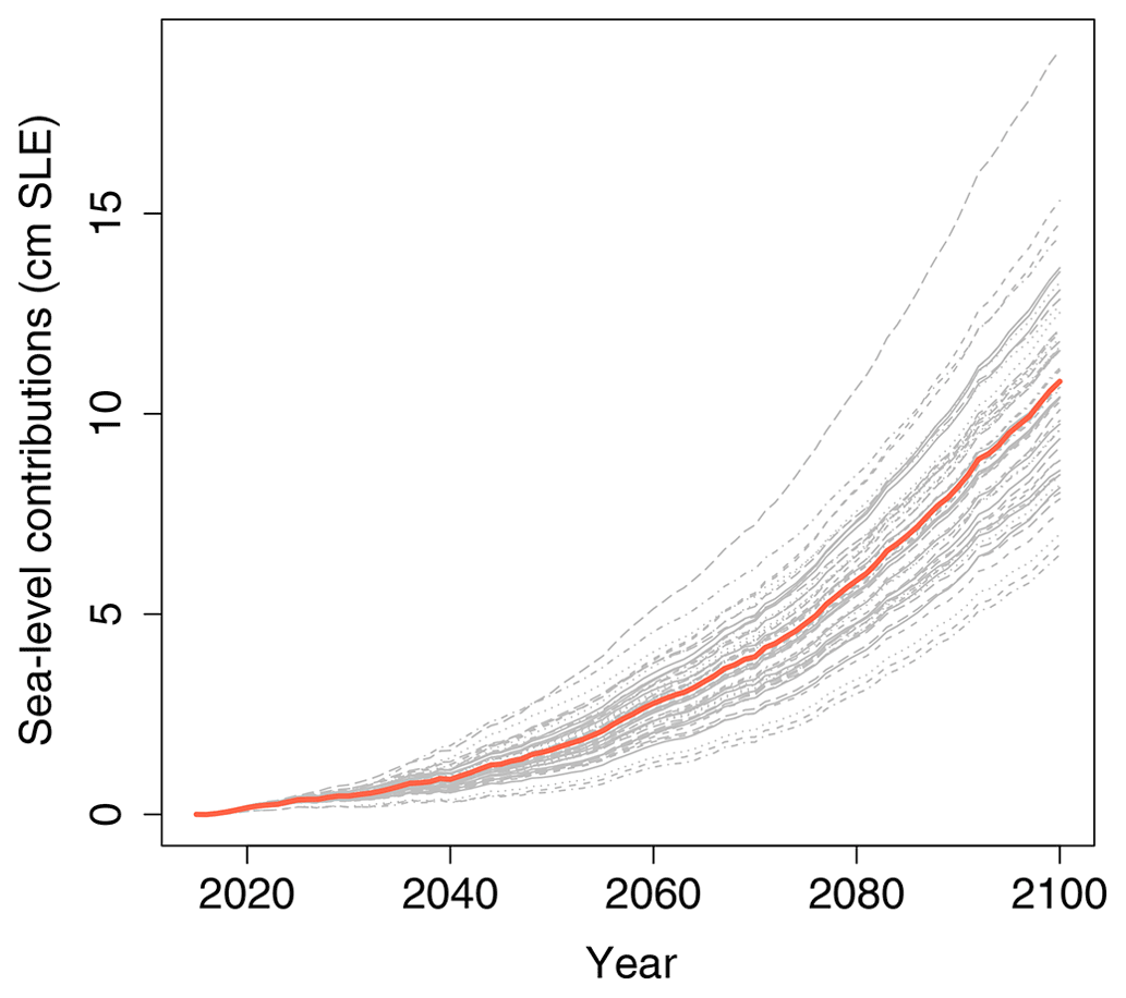
Figure 1(a) Time evolution of the sea-level contribution (with respect to 2015) from the Greenland ice sheet (in cm sea-level equivalent, SLE). The results are the MIROC5 RCP8.5-forced MME of Goelzer et al. (2020). The straight red line is the temporal ensemble mean.
The analysis is focused on nine main modelling assumptions related to different aspects of the modelling chain (Table 1), namely numerical implementation, initial conditions, modelling of ice-sheet processes, and environmental forcing. Only the modelling assumptions that are commonly shared by all models described by Goelzer et al. (2020) in their Appendix A were considered, i.e. without an empty entry in Table A1 in this paper. Note that some preliminary groupings of categories were carried out to ensure a minimum of variation across the experiments with at least two experiments associated with a given category (specified in the last column of Table 1), which is needed to properly conduct the performance analysis of the ML model (see further details in Sect. 3.2).
Table 1Modelling assumptions considered in the MIROC5 RCP8.5-forced GrIS MME.
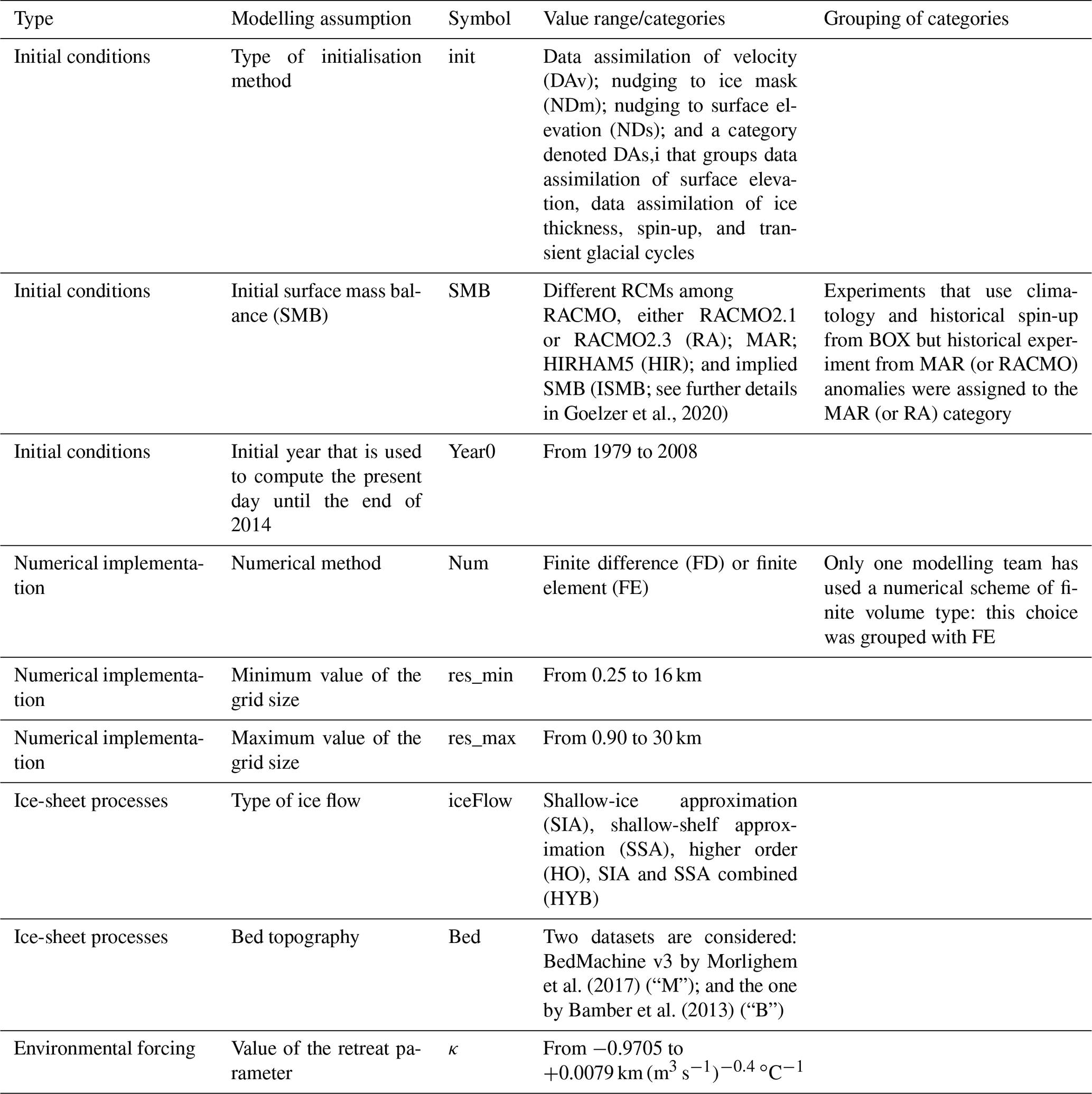
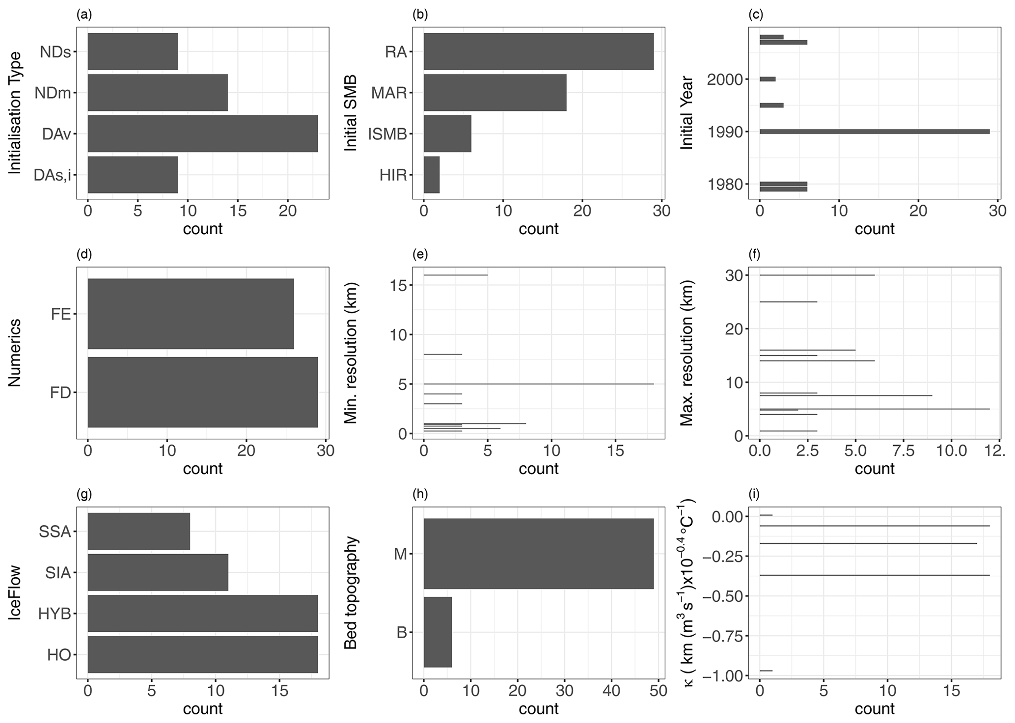
Figure 2Count number of the MIROC5 RCP8.5-forced GrIS MME members with respect to the different modelling assumptions described in Table 1.
In the following, we name the choices made for each of these modelling assumptions inputs. One input setting defines an experiment of the MME. Formally, the inputs are treated either as continuous variables (for κ, minimum and maximum resolution and initial year) or as categorical variables (for the five other ones). Figure 2 shows that the design of experiments is unbalanced: some categories (like RA for instance, Fig. 2b) or some values (like minimum resolution at 5 km, Fig. 2e) are more frequent than others. The design is also incomplete with large gaps in the histograms. This is for instance the case for κ between −0.9705 and −0.3700 km (m3 s ∘C−1 (Fig. 2i) because this parameter was sampled for only three different values by most models (the median, the 25th and the 75th percentile), and the additional two values were only sampled by one ISM.
3.1 Overall procedure
Let us consider sl(t) the sea-level change (with respect to a reference date) at a given time t that is numerically simulated from the chain of models, denoted f, described in Sect. 2. We assume that the different models (part of the MME) share the same characteristics corresponding to p different modelling assumptions (e.g. choice in initial SMB or ice flow formulation, value of the grid size). In our case p=9 (see Sect. 2). To each of these modelling assumptions is assigned a random variable x. The vector of p input variables (p modelling assumptions) is denoted by . We consider n different experiments, each of them associated with a particular x(i). The MME results at a given time t are with sl(i)(t)=f(x(i)). This means that our knowledge on the mathematical relationship f is only partial and based on the n MME results. To overcome this difficulty, we replace f by a machine-learning-based proxy (named the ML model) built using the MME results, the advantage being to make some predictions for input configurations that are not present in the original MME dataset at a low computation time cost. The ML model is denoted where θ correspond to the ML model's parameters (named hyperparameters; see Appendix B). Given a specific setting x∗ (i.e. an instance of modelling choices made by the modellers for each of the considered assumptions), we follow the additive feature attribution approach that has been developed for ML models (e.g. Štrumbelj and Kononenko, 2014; Lundberg and Lee, 2017). This approach proposes improving the interpretability of a particular prediction f(x∗) for a given time horizon t by decomposing it as a sum of the inputs' contributions (specific to x∗) as follows:
where μ0(t) (named the base value) is a constant value (see definition in Sect. 3.3).
It is important to note that Eq. (1) does not aim to linearise f but to compute the contribution of each input to the particular prediction value f(x∗). This means that the decomposition provides insights into the influence of the particular instance of the inputs x∗ relative to f(x∗): (1) the absolute value of μ∗(t) informs the magnitude of the influence at time t directly expressed in physical units (for instance in centimetres for sea level), which eases the interpretation; (2) the sign of μ∗(t) indicates the direction of the contribution, i.e. whether the considered modelling assumption pushes the prediction higher or lower than the base value μ0(t).
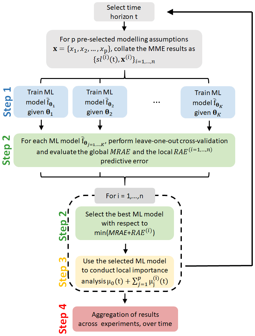
In order to quantify μ∗(t) in Eq. (1), the different steps of the proposed approach (schematically represented in Fig. 3) are as follows.
-
Step 1, build and train ML models. At a given time horizon t, an ML model is built using some supervised ML techniques (see Hastie et al., 2009, for an overview). We rely here on three types of ML models, namely a linear regression (denoted LIN) model (because of the simplicity of its implementation) and two tree-based approaches, a random forest regression method, denoted RF (Breiman, 2001), and extreme gradient boosting for regression, denoted XGB (Chen and Guestrin, 2016), which have shown high performance in diverse benchmark exercises (e.g. Grinsztajn et al., 2022, and references therein). See Appendix B for further details on these techniques and their respective hyperparameters θ.
-
Step 2, evaluate the predictive capability and select the best-performing ML model. The decomposition described in Eq. (1) is only meaningful provided that the assumption of replacing f with is valid. From this perspective, we propose assessing this assumption's validity by measuring the predictive capability of using a leave-one-out cross-validation procedure (Hastie et al., 2009). This validation is performed by considering the different parametrisations of the ML methods; i.e. the validation is performed by considering different values of the hyperparameters θ for each of the considered ML models. Two indicators are computed, namely a local one related to the considered ith MME result, which measures the relative absolute error (denoted RAE(i)), and a global one (denoted MRAE) defined as the average value of the RAE(i) values computed across all n MME results. Then, for the ith MME result, the ML model that performs the best with respect to the minimum value of MRAE + RAE(i) (i.e. both globally and locally for the considered ith MME result) is retained for the next step. The results of Step 2 are also useful to characterise the ML prediction error. Further details are provided in Sect. 3.2.
-
Step 3, local importance analysis. This step aims to perform the additive decomposition (Eq. 1) using the selected ML model. Among the different available methods (Molnar et al., 2020), we rely on the SHAP approach proposed by Lundberg and Lee (2017) because of its strong theoretical basis (see further details in Sect. 3.3 as well as Aas et al., 2021, their Appendix A, for a description from a modeller's perspective) as well as its multiple use in various application areas (see Introduction). Special care is given to the impact of the inputs' dependence by application of methods described in Sect. 3.4.
-
Step 4, summarise local explanations. The local explanations are combined and aggregated to provide insights into the model structure and to inform the sensitivity of sl(t) to the modelling assumptions at each time horizon t. Inspired by Lundberg et al. (2020), the sensitivity analysis is conducted at different levels:
-
Level 1, locally at a given prediction time. The value and sign of are analysed for a particular experiment. An application is provided in Sect. 4.3.1;
-
Level 2, model structure at a given prediction time. How the influence measured by (magnitude and sign) evolves as a function of the ith input value is analysed. An application is provided in Sect. 4.3.2.
-
Level 3, globally over time. How the magnitude of the influence measured by evolves across time is analysed by considering all experiments. To be able to compare the influence between the different predictions across time, we preferably analyse the absolute value of a normalised version of μ∗; i.e. . An application is provided in Sect. 4.3.3.
-
3.2 Predictive capability of the ML models
The objective of this section is to assess the validity of replacing f by an ML model (with θ being the ML hyperparameters). To do so, we aim to quantify the predictive capability of , i.e. whether is capable of predicting sl with high accuracy given yet-unseen instances of the modelling assumptions (inputs). If this predictive capability is high, replacing f with can be considered a valid assumption. The predictive capability of the ML model is commonly assessed using some global performance indicators calculated for a given test set T. Ideally, the analysis can be performed by defining an independent test set T in addition to the MME results. In the absence of such an independent dataset, we preferably rely on a leave-one-out cross-validation procedure (Hastie et al., 2009) that uses part of the available MME results to train the ML model and a different part to test it. At a given time t, the procedure holds as follows.
-
Step 1. Extract the ith MME result.
-
Step 2. Train using the other n−1 parts of the data, and the prediction error measured by is calculated when predicting the ith part of the data.
-
Step 3. The procedure is re-conducted for , and performance indicators are calculated by combining the n estimates of the prediction error.
We use two performance indicators, namely a local one that measures the local predictive capability related to the considered ith MME result and a global one that measures the predictive capability computed across all n MME results. The interest is twofold: the local indicator gives confidence in the local importance analysis for the considered ith case, and the global one gives confidence in the computation of the Shapley values, which require making predictions for inputs' configurations that are not necessarily present in the original MME dataset (see Sect. 3.3 and 3.4).
On the one hand, the local performance indicator is chosen to be the absolute error AE(i)(t)=|e(i)(t)|. To be able to compare the results across time and across the experiments, its normalised version will also be used, i.e. the relative absolute error . On the other hand, the global performance indicator is chosen to be the mean absolute error (and by its normalised version, the mean relative absolute error . For a given case i and at a particular time t, the ML model that minimises MRAE+RAE(i) is then retained for the local explanation analysis described in Sect. 3.3. This means that only the ML model that performs the best both globally (across the n MME results) and locally (for the considered ith MME result) is selected for the local explanation analysis.
Finally, it should be noted that no matter how much effort is put in increasing the ML predictive capability, a perfect match to the true model is rarely achievable, in particular due to difficulties in approximating the mathematical relationship between the inputs and sl or due to the absence of input variables that are important with respect to the sl prediction error. Thus, a residual degree of prediction error may still remain. This has implications for the interpretation of low values. In theory, means that the jth input has no impact on the prediction at time t; i.e. it has negligible influence. In practice, the absence of influence can be concluded only up to a given threshold that is related to the residual prediction error. This means that low contribution values cannot be distinguished from the predictive error. In the following, we propose using different performance indicators given the level of the sensitivity analysis (Step 4 described in Sect. 3.1) to assess the significance of the inputs' influence with respect to the prediction error: for Level 1, we use AE(i)(t); for Level 2, we use MAE(t); for Level 3, we analyse a variant of RAE(t), namely .
3.3 SHapley Additive exPlanations
We follow the approach developed by Lundberg and Lee (2017), who proposed defining in Eq. (1) using the Shapley value (Shapley, 1953). The Shapley value is used in game theory to evaluate the “fair share” of a player in a cooperative game; i.e. it is used to fairly distribute the total gains to multiple players working cooperatively. It is a fair distribution in the sense that it is the only distribution satisfying some desirable properties (efficiency, symmetry, linearity, “dummy player”; see proofs by Shapley, 1953; see Aas et al., 2021, their Appendix A for a comprehensive interpretation of these properties from an ML model perspective).
Formally, consider a cooperative game with k players and let be a subset of |S| players. Let us define a real-valued function that maps a subset S to its corresponding value and measures the total expected sum of payoffs that the members of S can obtain by cooperation. The gain that the ith player gets is defined by the Shapley value with respect to val:
Eq. (2) can be interpreted as a weighted mean over contribution function differences for all subsets S of players not containing player i. This approach can be translated for the ML-based sl prediction by viewing each model input (each type of modelling assumption) as a player and by defining the value function val as the expected output of the ML model conditional on , i.e. when we only know the values of the subset S of inputs (Lundberg and Lee, 2017); namely
where is the complement of S such that is the part of x not in xS and is the conditional probability distribution of given .
In this setting, the Shapley values can then be interpreted as the contribution of the considered input to the difference between the prediction and the base value μ0. The latter can be defined as the value that would be predicted if we did not know any inputs (Lundberg and Lee, 2017) and is chosen as the expected prediction for sl without conditioning on any inputs, i.e. the unconditional expectation μ0=E(f(x)). In this way, in Eq. (1) corresponds to the change in the expected model prediction when conditioning on that input and explains how to depart from E(f(x)). The interest is that the sum of the Shapley values for the different inputs is equal to the difference between the prediction and the global average prediction , which means that the part of the prediction value which is not explained by the global mean prediction is totally explained by the inputs (Aas et al., 2021, their Appendix A). This has several implications in the MME context: (1) any input will be assigned a Shapley value (defined by Eq. 2); (2) if , it indicates the absence of influence for the ith input (related to the dummy player property of the method); (3) the sum of the inputs' contributions is guaranteed to be exactly (related to the efficiency property of the method). This also means that the selection of the input variables in the analysis is an important step because the quantified contributions are dependent on the choice of which input variables are included in the analysis (see Discussion, Sect. 5).
In practice, the computation of the Shapley value may be demanding because Eq. (2) implies covering all subsets S (which grow exponentially with the number of factors denoted k, i.e. 2k) and Eq. (3) requires solving integrals, which are of dimension 1 to k−1. For both reasons, the calculation is performed using a surrogate model (i.e. the ML model) in place of the true function f because the design of computers is rarely complete (i.e. it rarely contains the results for the different configurations of the inputs that are needed for the calculation). To further alleviate the computational burden in this study, we rely on the kernel SHAP method of Lundberg and Lee (2017), which allows a computationally tractable approximation, and a simple method for estimating the value function in Eqs. (2)–(3). For this purpose, we use the R package “shapr” (Sellereite and Jullum, 2020), which accounts for inputs' dependencies (see Sect. 3.4).
3.4 Accounting for inputs' dependencies
In the case considered in this study, there exists some dependence among the inputs. A commonly encountered example is when the values for the minimum and maximum grid sizes are correlated. Additional examples are provided in Sect. 4.1. In this case, the interpretation of the SHAP decomposition provided by the kernel SHAP method might give wrong answers (Aas et al., 2021) because it relies on the independence assumption for calculating the conditional probability in Eq. (3). In our case, the dependence cannot be neglected (see Sect. 4.1 for the application to the GrIS MME), and we rely on the improved kernel SHAP method proposed by Redelmeier et al. (2020) using conditional inference trees, denoted CTREE (Hothorn et al., 2006), to account for the dependence structure of input variables that are of mixed types (i.e. continuous, discrete, ordinal, and categorical) in the calculation of Eq. (3).
Conditional inference trees belong to the class of decision trees that use a two-stage recursive partitioning algorithm, namely (1) partitioning of the observations by univariate splits in a recursive way and (2) fitting a constant model in each cell of the resulting partition (for the regression problem). Different splitting procedures exist, and here we use the one proposed by Hothorn et al. (2006) that uses a significance test to select input variables rather than selecting the variable that maximises the information measure (such as the Gini coefficient; Breiman, 1984). In this approach, the stopping criterion is based on p values of the significance test; for instance the p value must be smaller than a given value (typically of 5 %) in order to split the considered node. The advantage of CTREE is to avoid a selection bias towards covariates with many possible splits or missing values (see Hothorn et al., 2006, for further details).
To identify the dependence structure, we proceed as follows. We first consider the first input variable to be the response and fit a CTREE model by viewing the remaining input variables as the predictor variables. If the resulting tree model includes one of the predictor variable, this means that there is some dependence with the considered response (i.e. the first variable in this example). Otherwise, the resulting tree model is empty. This approach is re-conducted by considering each of the input variables as the response in turn. As a result, the procedure identifies the non-empty tree model or models that represent the dependence structure between some input variables.
In this section, we apply the procedure described in Sect. 2 (schematically depicted in Fig. 3) to the MIROC5 RCP8.5-forced GrIS MME. We first analyse the dependence between the different modelling assumptions (Sect. 4.1). Then, we train and build ML models and select the best-performing ones by following Steps 1–2 of the procedure (Sect. 4.2). On this basis, we apply the local attribution approach to measure the local importance and summarise the results to provide different levels (detailed in Sect. 3.1) of information on sensitivity (Steps 3–4, Sect. 4.3).
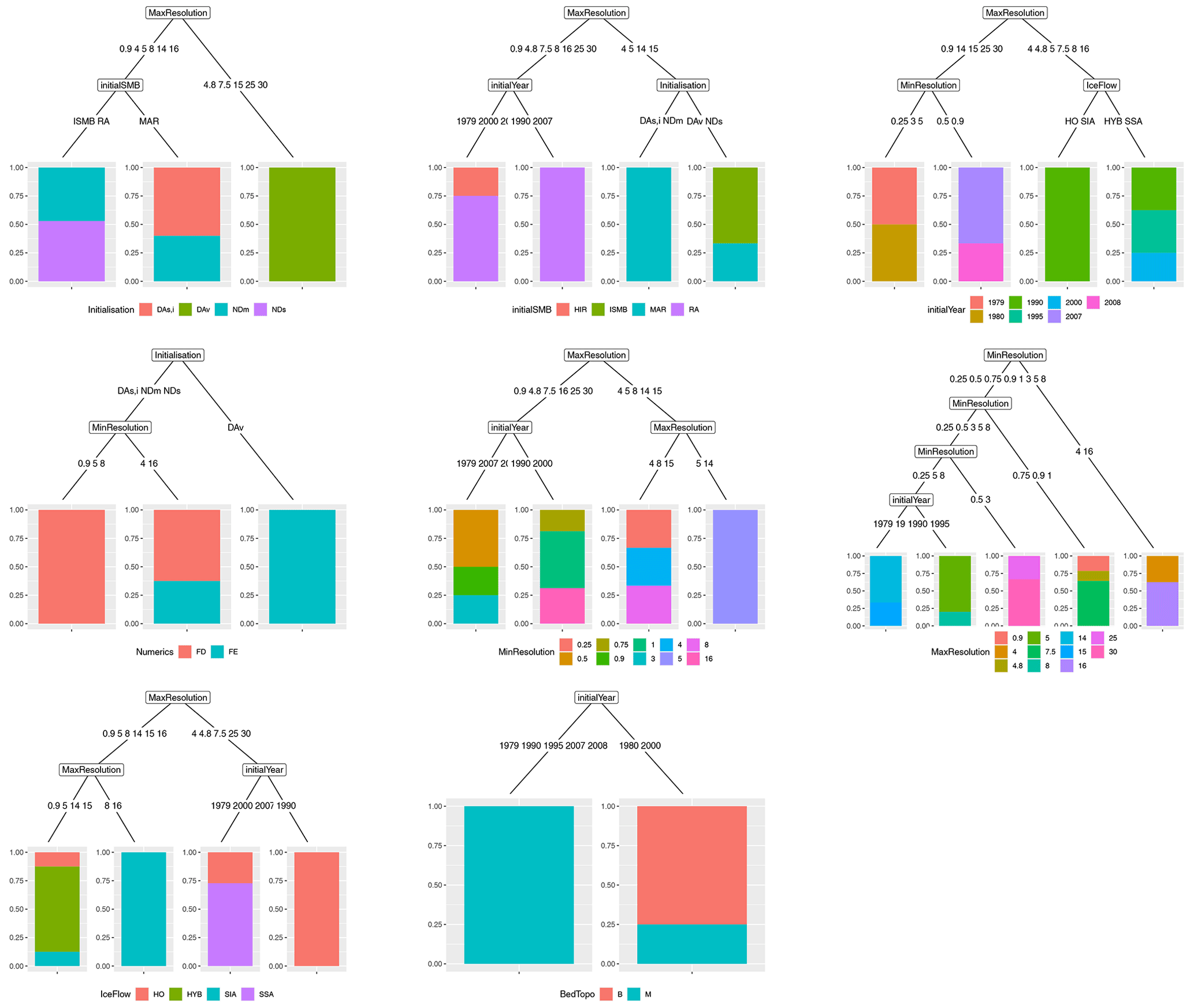
Figure 4Tree models representing the dependence between the different modelling assumptions (indicated at the bottom of each tree). The bottom nodes (leaf nodes) provide the proportion of experiments given the modelling choices defined along the branches of the tree model. Each colour corresponds to a different category of the considered modelling assumption. For instance, the left tree in the middle row provides the relation between the choice in the numerical method with the type of initialisation and the minimum grid size. The blue (red) colour is related to the finite element FE (finite difference FD) category.
4.1 Inputs' dependencies
We first analyse the statistical dependence among the modelling assumptions (inputs) by applying the CTREE approach described in Sect. 3.4 (using a split criterion threshold of 95 % and Bonferroni-adjusted p values). Figure 4 shows the resulting tree models for the different modelling assumptions. We show here that all inputs are statistically dependent with the exception of κ for which the tree model is empty, which indicates the absence of (significant) dependence between this parameter and the other modelling assumptions. The different tree models should be read by following the example of the leftmost tree in the middle row of Fig. 4. This tree provides the relation between the choice in the numerical method with the type of initialisation and the minimum grid size. The bottom nodes (leaf nodes) provide the proportion of experiments given the combination of modelling choices defined along the branches of the tree model. The blue (red) colour is related to the finite element FE (finite difference FD) category. This tree model indicates for example that all models with initialisation of type DAv have a numerical method of type FE (rightmost branch) and all models with initialisation different from DAv and a minimum resolution of 0.9, 5, or 8 km have a numerical method of type FD (leftmost branch).
4.2 Predictive capability of the ML models
Using the results of the MIROC5 RCP8.5-forced GrIS MME, we train a series of ML models to predict sl across time. The following ML models with corresponding hyperparameters (see Appendix B for details) are considered:
-
9 RF regression models with hyperparameters ns = 5 or 10; mtry=1, 3, 6, or 9; and ntree=2000;
-
30 XGB models with hyperparameters maximum depth = 2, 3, 6, or 9; learning rate = 0.025, 0.1, or 0.25; and maximum number of boosting iterations = 250 or 450;
-
1 LIN model.
To assess the predictive capability of the considered ML models at each time instant, we apply a leave-one-out cross-validation approach by following the procedure of Sect. 3.2. Figure 5a depicts the time evolution of the performance indicator MRAE for all considered ML models. Depending on the type of ML model (and corresponding parametrisation), the global performance can reach satisfactory levels below 10 %, in particular for some XGB models.
As explained in Sect. 3.2, satisfying the global performance criterion does not necessarily ensure that the ML model gives an accurate approximation of all sl predictions. For some cases, the discrepancies can be too large to properly analyse the local explanations. This is illustrated with Fig. 5b, which shows the comparison between the true sl value and the corresponding ML-based prediction for 2100. For instance, we note that the predictions for the largest sl value largely depart from the 1:1 line except for the LIN model (outlined in black in Fig. 5b). This is also the case for the lowest sl values for which a given parametrisation of the XGB model performs the best (outlined in red in Fig. 5b). Thus, to further increase our confidence in replacing the “true” numerical model by the ML model, we apply the filtering approach (described in Sect. 3.2) based on the joint minimisation of the global and of the local performance indicators. The retained predictions are outlined in blue in Fig. 5b.
In total, LIN, XGB, and RF models retained 3.4 %, 24.6 %, and 72 % respectively of the total number of experiments (on average over time). After applying this procedure, the MRAE criterion (shown in blue in Fig. 5a) reaches values below 10 % on average over time (with a maximum value not larger than 15 % for the year 2040). Note that the MRAE curve after this selection is not necessarily the lowest one because the selection procedure implies minimising not only MRAE but also the local performance RAE(i) (see Sect. 3.2).
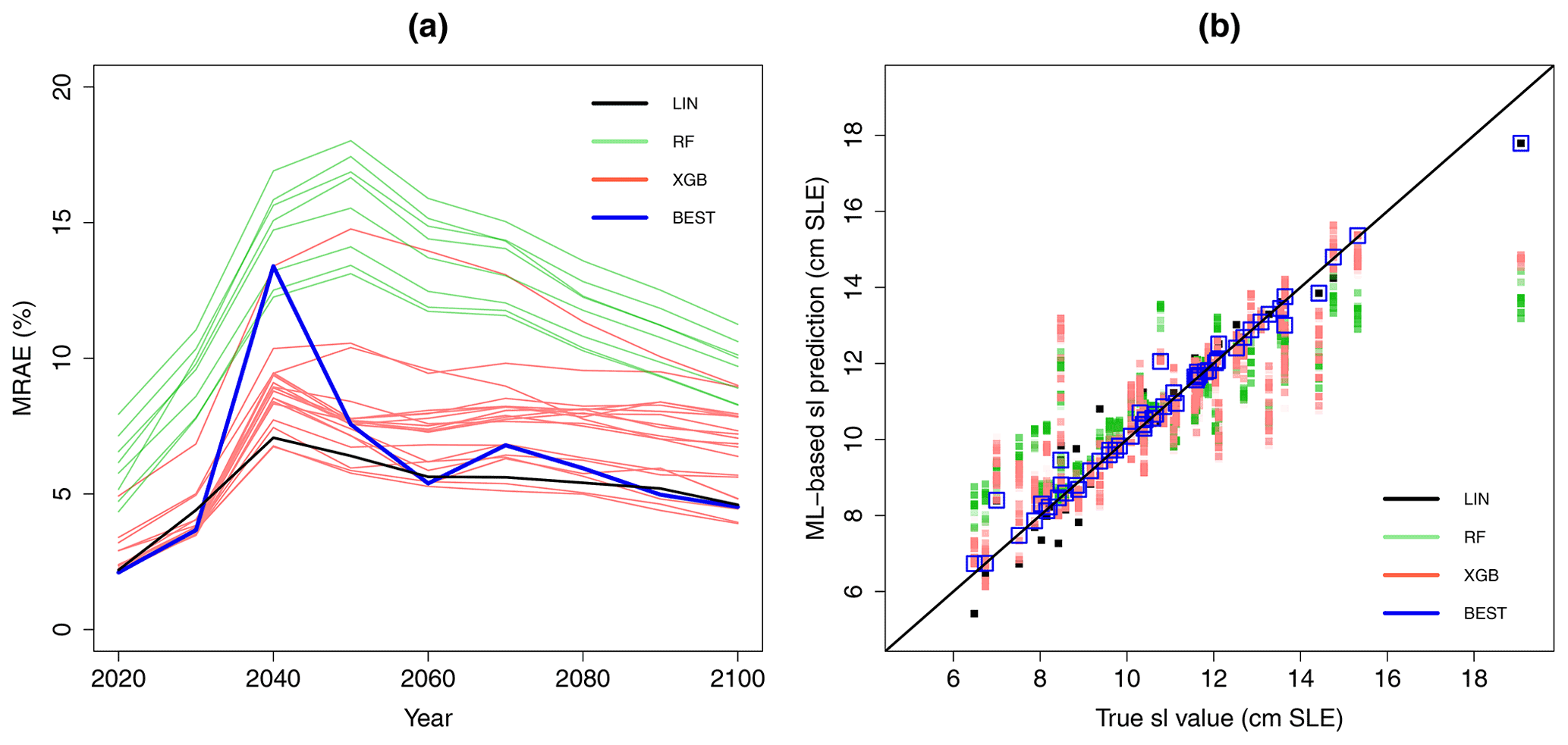
Figure 5(a) Time evolution of the performance criterion MRAE (expressed in %) computed using a leave-one-out cross-validation procedure that assesses the predictive capability of all considered ML models with different parametrisations (RF models in green, XGB in red, and LIN in black). The blue-coloured lines are related to the performance criterion after selecting the best-performing ML model with respect to the joint minimisation of the global and of the local performance indicator described in Sect. 3.2; (b) comparison between the true and the ML-based predicted sl value for 2100 by considering all ML models. The blue-coloured squares outline the retained results after selecting the best-performing ML model.
4.3 From local to global explanations
In this section, we first compute the measures of local importance for each experiment in the MIROC5 RCP8.5-forced GrIS MME for a given prediction time (here 2100); such a type of diagnostic (Level 1 of the procedure) helps to understand and quantify the impact of particular assumptions made by the modellers (Sect. 4.3.1). Then, we analyse in Sect. 4.3.2 how the influence of each modelling assumption evolves as a function of the considered input value (Level 2 of the procedure). This analysis allows us to deepen our understanding of the model structure for a given prediction time. Finally, Sect. 4.3.3 summarises all results over time (Level 3 of the procedure) to provide a global insight (i.e. across all MME members) into the sensitivity of sl to the modelling assumptions.
4.3.1 Level 1: local explanations at a given prediction time
We first illustrate the application of SHAP to a selected set of ML-based sl predictions for 2100. Figure 6 provides the SHAP-based decomposition of the ML-based prediction (horizontal blue bar) into the positive (green bar) or negative (red bar) contribution (μ value defined in Eqs. 2–3) of each input using the 2100 ensemble mean of μ0=10.8 cm as a base value. The inputs' setting are indicated on the vertical axis for each of the cases considered: Cases (a)–(f). The grey colour indicates that the contribution cannot be distinguished from the predictive error because its absolute value is below the absolute error.
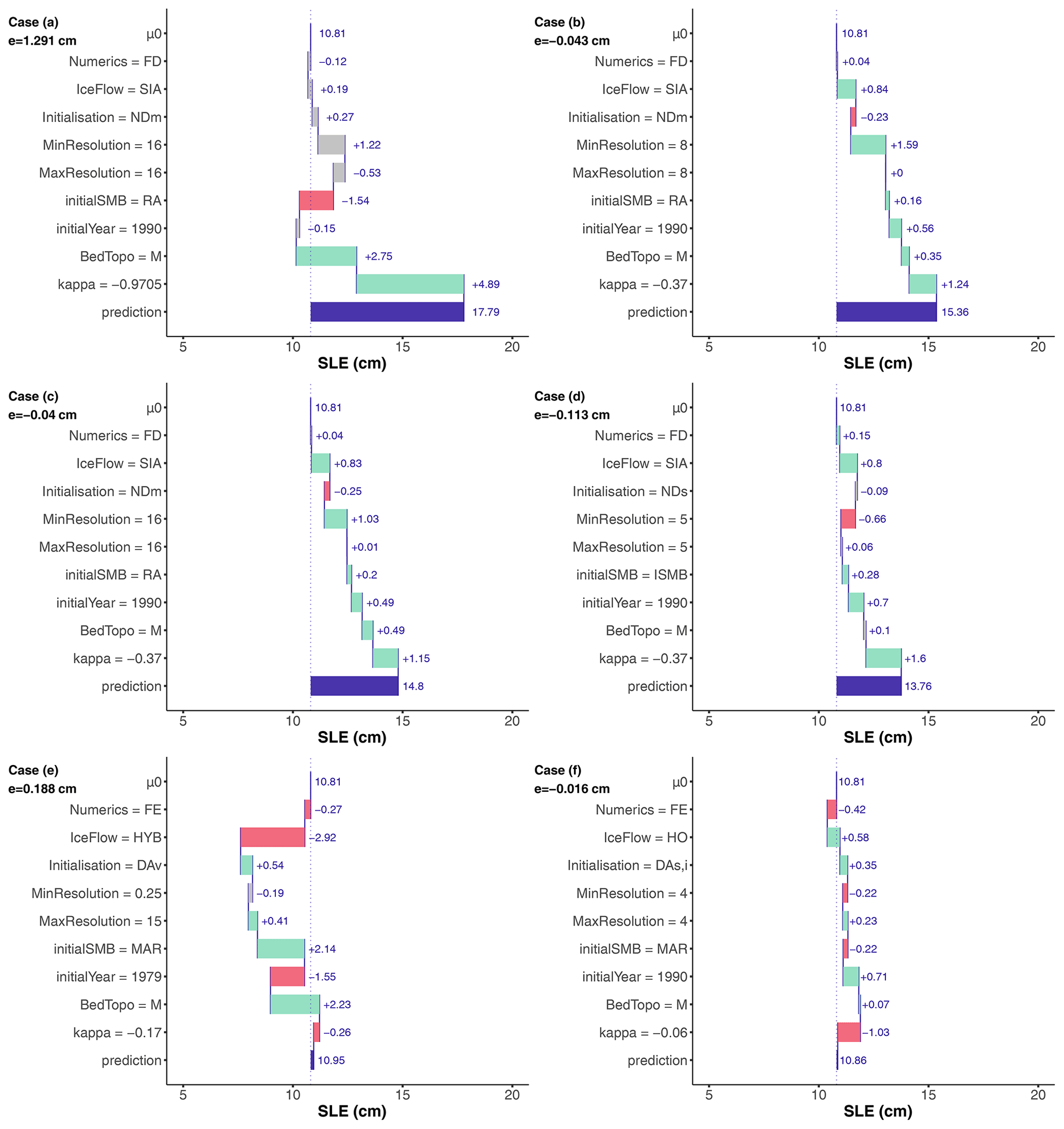
Figure 6Diagnostic of particular ML-based sl predictions using SHAP for the year 2100 considering six different settings of the modelling choices (indicated on the vertical axis). The horizontal blue bar corresponds to the ML-based sl prediction (the difference with the true value is indicated by the error term e expressed in cm SLE). Each row shows how the positive (green bar) or negative (red bar) contribution of each input moves the prediction from μ0, i.e. the unconditional expectation of sl. The grey colour indicates that the contribution cannot be distinguished from the predictive error because its absolute value is below the absolute error.
The analysis of Fig. 6 illustrates how the SHAP-based approach can be used to diagnose the MME results.
-
Case (a) corresponds to the largest sl value (of 19.08 cm) that is predicted by the ML model at 17.79 cm (with a prediction error e≈1.30 cm). Figure 6a confirms the physically expected result regarding κ influence: the largest sl is mainly attributable to the κ whose absolute value is the largest, i.e. 0.9705 km (m3 s ∘C−1. This choice pushes the sl value higher than the base value by .89 cm, i.e. by ≈ 45 % of μ0. In this case, the two other largest contributors to sl (with an influence of +2.75 and −1.54 cm respectively) are related to using the M dataset for bed topography and initial SMB of type RA. The other modelling choices all have absolute contributions below , which indicates that their contributions are not significant in comparison to the prediction error level (outlined in grey in Fig. 6a).
-
Case (b) (Fig. 6b) corresponds to the second-largest sl value (of 15.32 cm) that is predicted by the ML model at 15.36 cm (with a prediction error e≈0.04 cm). All modelling choices are similar to Case (a) except κ, here set to a lower absolute value of 0.37 km (m3 s ∘C−1, and with the minimum grid size set to a lower value of 8 km. Contrary to Case (a), the influence of κ drops here to a low to moderate value (+1.24 cm), and it is the choice of the minimum grid size that contributes the most to sl (1.59 cm). We note that all contributions can be considered with confidence because their absolute values are all above the absolute prediction error.
-
Case (c) has the same setting as Case (b) except for a larger minimum grid size (here of 16 km). This results in a lower influence of the minimum grid size (μ drops to +1.03 cm), but the contributions of all modelling assumptions remain, to some extent, similar to Case (b).
-
Case (d) corresponds to an sl value close to the one in Case (c) and illustrates that, despite the differences with Case (c) (i.e. initial SMB, initialisation type, and minimum resolution), the contribution of the largest contributors to sl, i.e. ice flow type, initial year, and κ, remains of the same order of magnitude between both cases.
The comparison between Cases (b) to (d) also points out that, for relatively close predicted values, the modelling choices contribute equivalently to the prediction despite some minor differences in the setting of the modelling assumptions.
-
Cases (e) and (f) illustrate however that, when the dissimilarity in the settings is larger, the modelling choices contribute differently to the prediction although the predicted values are very close (here close to the ensemble mean of 10.8 cm). In Case (f), all modelling assumptions contribute equivalently to sl, whereas it is mainly ice flow type and the type of dataset for bed topography in Case (f).
Such a type of diagnostic can be performed for any MME results (they are all provided by Rohmer, 2022, for the year 2100) to inform the modellers about the most and least impactful modelling choices for any sl prediction, such information being helpful to explain why a given instance of modelling choice leads to a given sl value.
4.3.2 Level 2: model structure at a given prediction time
We explore in Figs. 7 and 8 how the magnitude of the modelling assumption's contribution to sl, as well as the direction, changes depending on the value of the considered input by applying the SHAP dependence plot proposed by Lundberg et al. (2020). To judge the significance of the contribution, we compare the results to the range defined by ±MAE = 0.18 cm (calculated from the leave-one-out cross-validation procedure; see Sect. 4.2): contributions falling within this range (outlined by the dashed horizontal red lines in Fig. 7) indicate that they cannot be distinguished from the predictive error.
We first analyse the continuous variables. Figure 7a confirms the large influence of κ (of several centimetres) for large absolute values of κ. We also note that setting this parameter to −0.17 km (m3 s ∘C−1 leads to a quasi-negligible influence because μ falls within the range of MAE. A clear trend can be noticed: κ influence decreases with increasing value in a quasi-linear manner (with a slope of 8 cm per unit of retreat parameter). We also note that setting κ above −0.17 km (m3 s ∘C−1 even impacts negatively the sl prediction, which means that this modelling assumption pushes the prediction lower than the mean value for 2100. Finally, Fig. 7a provides indication of where to perform additional numerical experiments to confirm the influence of κ, namely over the range −0.97 to −0.37 km (m3 s ∘C−1 (where the results are scarce).
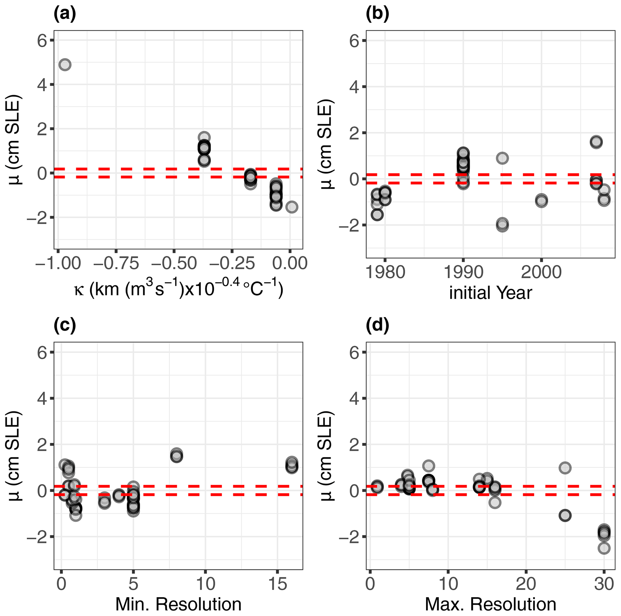
Figure 7Application of SHAP to all members of the MIROC5 RCP8.5-forced GrIS MME for the year 2100. Each panel provides μ (y axis) as a function of the value of the minimum and maximum grid resolution (c, d), of the initial year (b), and of the retreat parameter κ (a). The horizontal dashed red lines indicate the limits defined by ±MAE calculated from the leave-one-out cross-validation procedure: contributions falling within this range indicate that they cannot be distinguished from the predictive error.
Though a trend in the (initial year – μ) mathematical relationship is not straightforward to detect, Fig. 7b shows that the influence can be considered significant with respect to the predictive error MAE for some particular cases; reaches low to moderate values not larger than 2 cm.
Figure 7c and d give insights into the influence of the spatial resolution by showing a zone of low-to-moderate influence defined for a minimum and a maximum grid size < 5 and < 16 km respectively. In this zone, the average value of across the cases is 0.55 and 0.27 cm for the minimum and maximum resolution respectively (with a maximum value of up to ≈ 1.1 cm for both grid sizes). The influence can even be considered non-significant with 40 % of the cases falling within the ±MAE range for the maximum grid size. From a modelling perspective, this analysis suggests that there is clear interest in running high-resolution simulations. This means that if spatial grid resolution is too coarse (i.e. if the minimum and maximum grid resolutions are outside the identified zone), this choice may highly influence the results of sea-level projections; can be as high as 1.60 and 2.50 cm for the minimum and maximum grid size respectively. A comparison with the contributions of the other modelling assumptions in Fig. 8 further suggests that the influence of spatial resolution may dominate all other modelling choices, since their contributions do not exceed +1 cm; i.e. they are smaller than those of the identified zone.
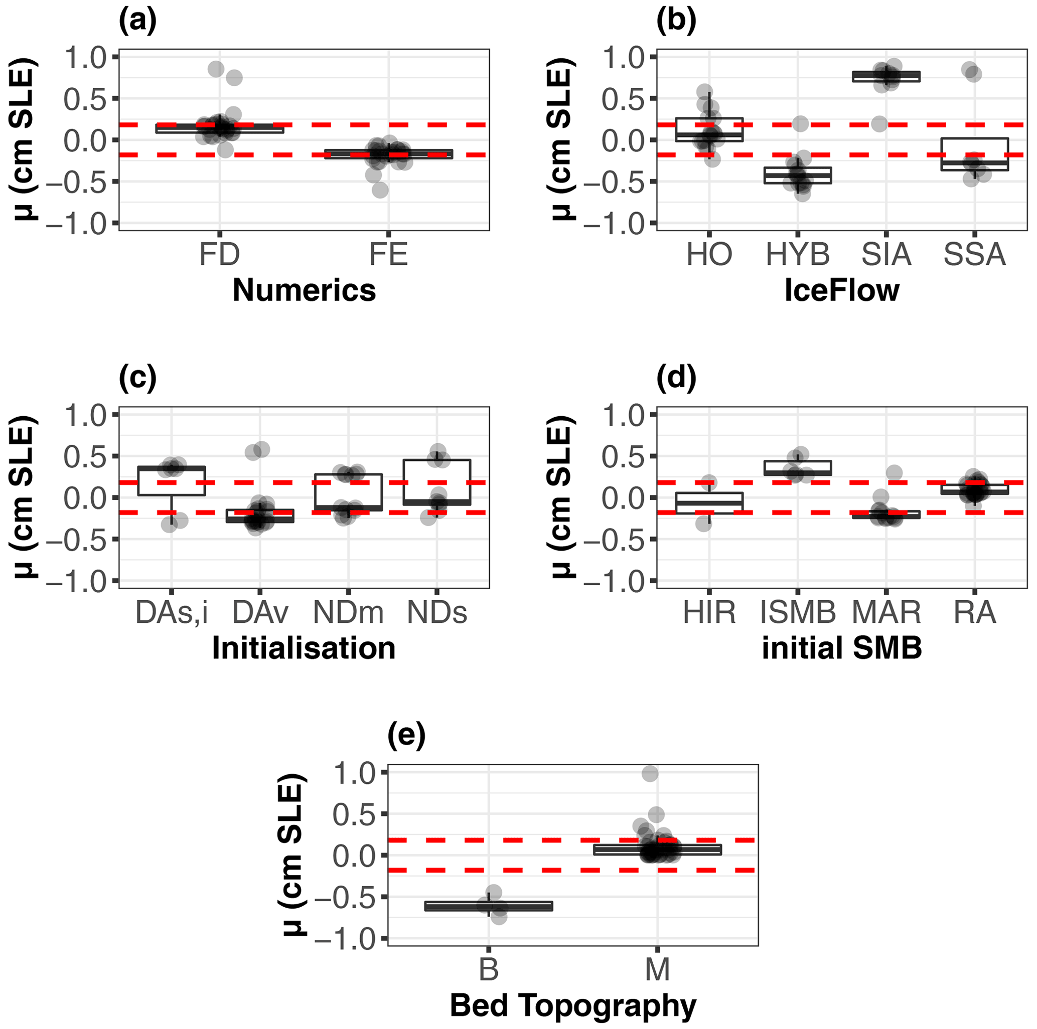
Figure 8Application of SHAP to all members of the MIROC5 RCP8.5-forced GrIS MME for the year 2100. Each panel provides the boxplots of μ values given the modelling choice for the numerical method (a), the ice flow (b), the initialisation (c), the initial SMB (d), and the type of bed topography dataset (e). Each dot corresponds to a given MME member. The horizontal dashed red lines indicate the limits defined by ±MAE calculated from the cross-validation procedure.
Focusing on the categorical input variables, Fig. 8 further indicates that the most impactful modelling assumption for sl is the ice flow choice, either of SIA or of HYB type with a positive or negative contribution, and the B dataset for bed topography: the corresponding boxplots in Fig. 8b and e are well outside the ±MAE range. Finally, Fig. 8 also highlights some modelling choices with contributions that are hardly distinguishable from the prediction error, namely any type of numerical method, FD or FE (Fig. 8a), NDm, and NDs for initialisation (Fig. 8c); HIR or RA for initial SMB (Fig. 8d); and the M dataset for bed topography though some specific cases present low-to-moderate values (see grey dots outside the box in Fig. 8e).
4.3.3 Level 3: global explanations over time
The analysis of Sect. 4.3.2 is now performed for all members of the MIROC5 RCP8.5-forced GrIS MME for any prediction time. As indicated in Sect. 3.1, to be able to compare the influence between the different predictions across time, we analyse in Fig. 9 the statistics of the absolute value of . To assess the negligible level of the influence with respect to the ML prediction error, we analyse the quartiles of calculated at each time instant for all members of the MIROC5 RCP8.5-forced GrIS MME. If the boxplot depicted in Fig. 9 does not overlap with the region defined by the interval between the lower and the upper red cross, this means that the influence measured by |μn| can be considered significant with respect to the ML prediction error.
Considering initial conditions, Fig. 9a and c show that it is the initialisation type that has the largest impact in the medium term (before 2050/2060), and after this date, it is the choice in the initial year that has the most impact. Conversely, in the long term (after 2050/2060), the influence of the initialisation type reduces up to a negligible level (compared to the prediction error). Figure 9b shows that the influence of the initial SMB is low (even negligible) regardless of the considered prediction time with the exception of some particular cases outlined by black dots lying outside the boundaries of the whiskers (these cases are illustrated in Fig. 6a, e).
Considering numerical implementation, the choice of the numerical method has here a small (even negligible) impact on sl values (Fig. 9d) especially in the medium/long term (after 2050). We note also that the moderate influence of the minimum and maximum grid size remains quasi-constant over time (Fig. 9e, f), hence suggesting that the grid size's influence is time-invariant; i.e. all modelled processes are affected by the spatial resolution in a similar way, independently of the prediction time.
Finally, considering ice-sheet processes and environmental forcing, an important influence of κ is shown only after 2030/2040 (Fig. 6h) with a quasi-constant value after this date. An increasing influence over time is also identified for the ice flow type, though the temporal trend is only clear up to the year 2070. We also show that the type of bed topography dataset has only a low (even negligible) influence compared to the prediction error, with the exception of some particular cases (illustrated in Fig. 6a, e) outlined by black dots lying outside the boundaries of the whiskers.
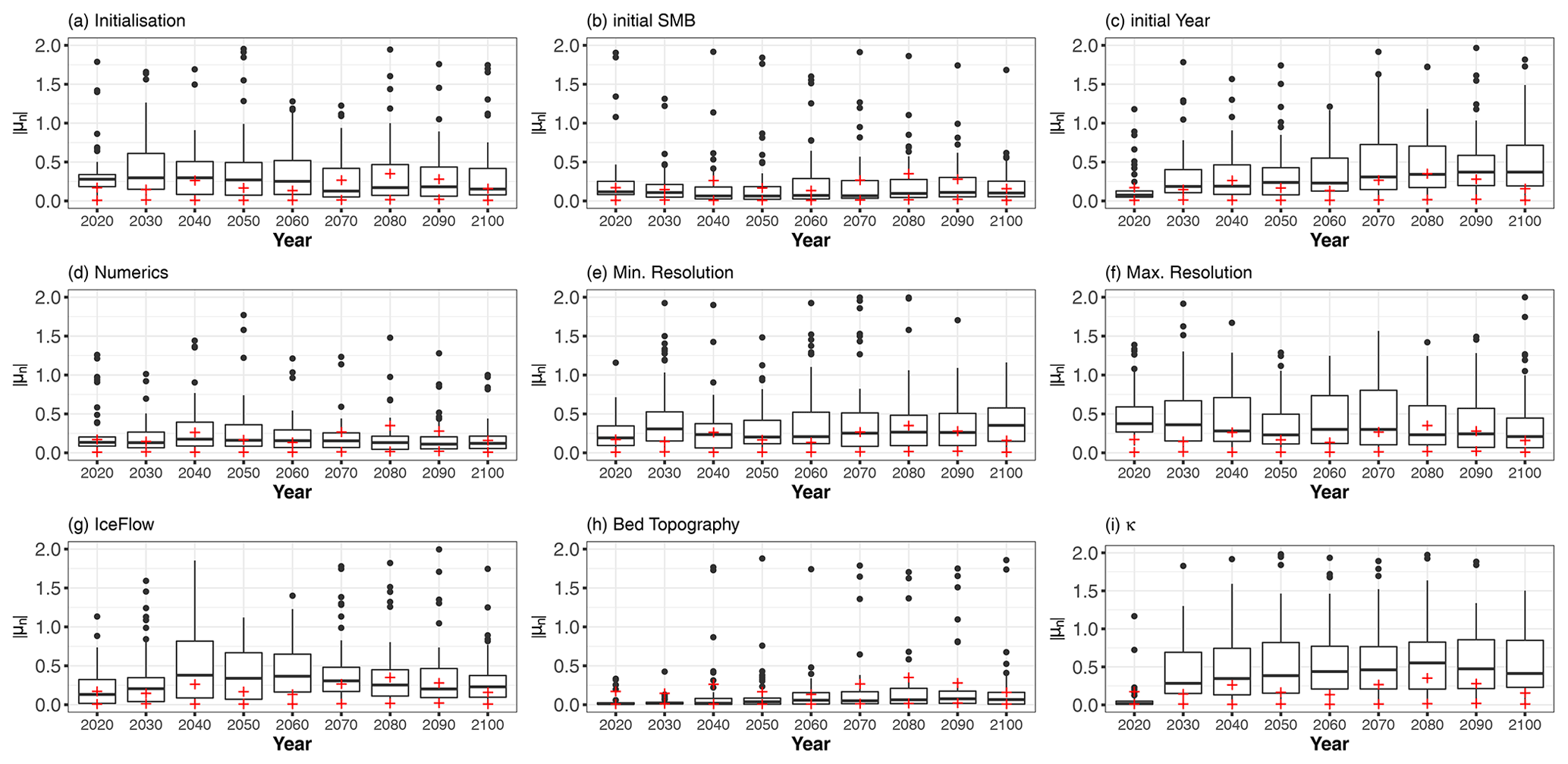
Figure 9Statistics of |μn| summarised by a boxplot at each time instant for all members of the MIROC5 RCP8.5-forced GrIS MME. The lower and upper red crosses are the first and third quartile respectively of the cross-validation error RAEn. If the boxplot does not overlap with the region defined by the interval between the red crosses, this indicates that the influence measured by |μn| can be considered significant with respect to the ML prediction error. For readability, the upper bound of the y axis has been set to 2.
Improving the interpretability of sea-level projections is a matter of high interest given their importance to support decision-making for coastal risk management and adaptation. To this end, we adopt the local attribution approach developed in the machine learning community to provide results about the role of various modelling choices in generating inter-model differences in the MME. These results are intended for different potential users.
First, the diagnostics illustrated in Fig. 6 (and all provided by Rohmer, 2022, for MIROC5 RCP8.5-forced GrIS MME in 2100) help the individual modellers involved in the modelling exercise to understand and quantify the impact of their particular assumptions. Figure 6b–d illustrate situations where the SHAP approach allows such critical analysis, including checking that the same modelling assumptions have a similar impact on close sl values.
Second, aggregating all diagnostic results (Level 2 and 3 of the proposed approach) provides guidance to the modelling group involved in the definition of experimental protocols for MMEs (such as ISMIP6; Nowicki et al., 2016, 2020). Some key aspects are identified and deserve to be taken into account in future model developments and modelling exercises.
-
Our results confirm the need for simulations that are sufficiently spatially resolved: sl results are largely affected by too coarse grids (here with a minimum and maximum grid size larger than 5 and 16 km respectively) regardless of the prediction time.
-
The influence of the modelling assumptions depends on the considered prediction time: in the short/medium term (before 2050), initialisation and ice flow type primarily contribute to sl, whereas in the long term, the initial year and κ are tagged as key contributors; though κ importance has a relatively well understood physical basis, additional analysis should be carried out for the initial year.
-
Some modelling choices have little impact on the sl values (on average across the considered MME results), in particular choosing a finite element or finite difference numerical scheme or the dataset for bed topography.
-
Additional computer experiments are worth conducting to better explore given parts of the parameter space with a view to confirming the identified trends (Figs. 7 and 8), in particular for a minimum grid size ranging from 3 to 4 km and for κ ranging from −0.97 to −0.37 km (m3 s ∘C−1.
Finally, framing the diagnostic results with narratives is expected to facilitate the communication between modellers and end users. What is “easily explained” through narratives is expected to increase the end user's level of trust in the model and eventually their engagement in the decision-making process (e.g. Jack et al., 2020). The narratives can follow the example of the GrIS study (Fig. 6a): “the largest sl predicted value is 19.1 cm by 2100 and is mainly attributable (by a positive factor of almost 50 % of the ensemble mean) to setting κ to its largest absolute value, i.e. a large contribution of outlet glacier retreat, while the other modelling assumptions have only moderate influence”. More broadly, this provides a clear message for risk-adverse stakeholders interested in the upper tails of the distribution (named “high-end” sea-level scenarios; Stammer et al., 2019), namely the importance of the dynamics of ice-sheet processes for projected high sl values, especially in the second half of the century. This message then calls for intensified future research work to reduce uncertainty related to these processes.
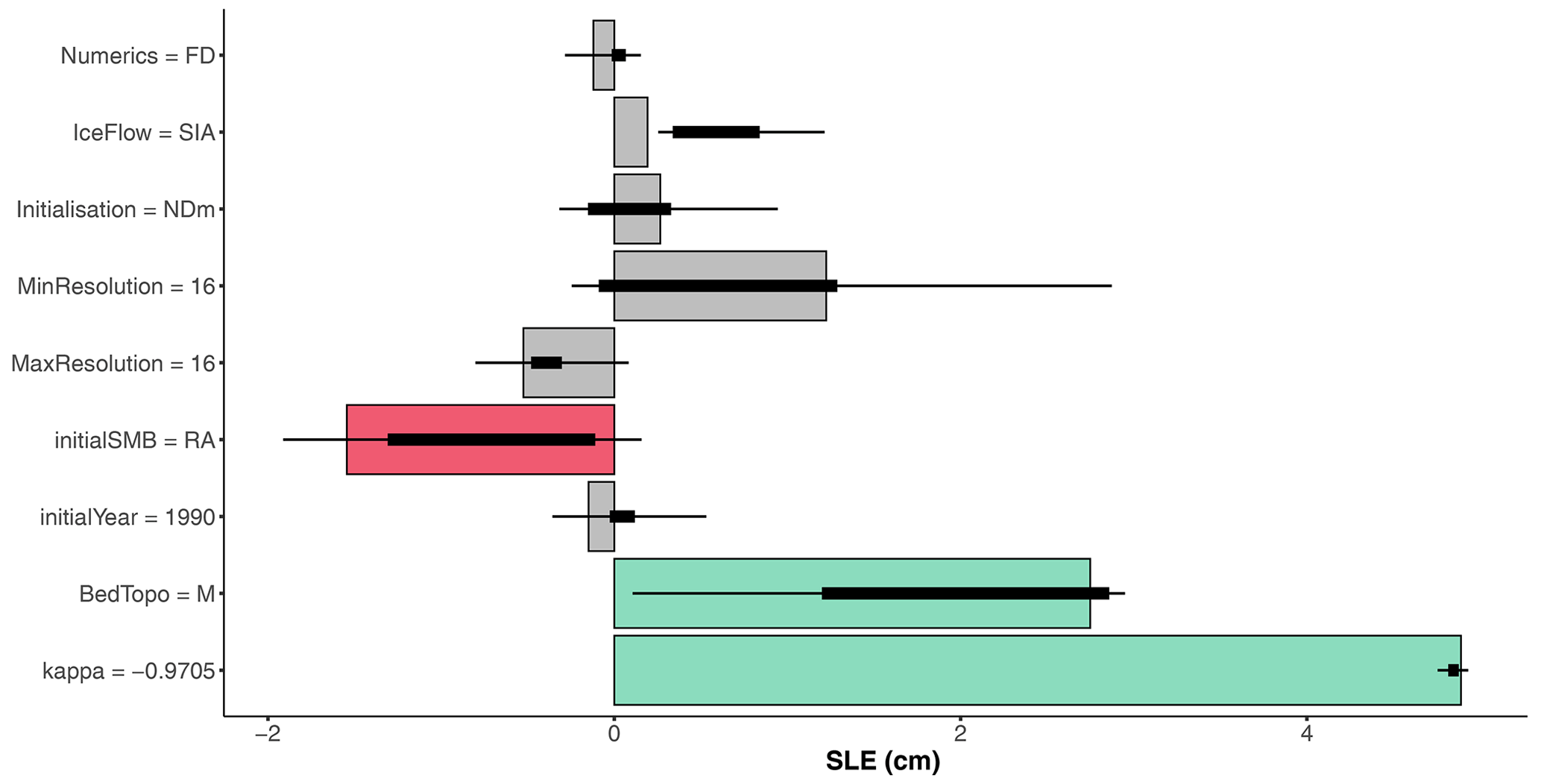
Figure 10Robustness analysis of the local importance analysis for the largest simulated sl value in 2100 (Case (a) in Fig. 6). The horizontal coloured bars correspond to the quantified contributions by including all input variables (results of Fig. 6a). The endpoints of the thick and thin horizontal black error bars are the minimum/maximum and the percentiles at 25 % and 75 % respectively computed when iteratively excluding one of the nine input variables.
These results were obtained by overcoming two major difficulties. The first one is related to the incomplete and unbalanced design of the numerical experiments (Sect. 4.1). Here, applying more commonly used statistical methods, namely the linear regression model or the ANOVA-based approach, would hardly be feasible. On the one hand, Sect. 4.2 clearly shows that the mathematical relationship between sl and the inputs is not necessarily linear, and more advanced regression techniques need to be used (like RF or XGB models). On the other hand, the considered design of experiments is incomplete and unbalanced (as shown in Sect. 2), which complicates the application of ANOVA. Ideally a full factorial design should be used to properly apply ANOVA: in our case, the design should then contain 3200 experiments, i.e. far more than the available number of experiments. Some solutions have been proposed in the literature (see, for example, Evin et al., 2019, and references therein), and an avenue for future work could focus on the comparison of ANOVA with our approach. The second difficulty is related to the presence of statistical dependencies (as outlined in Sect. 4.1), which makes the interpretation of the individual effects less straightforward (a problem related to multicollinearity in the statistical community, e.g. Shrestha, 2020) and might even lead to wrong conclusions regarding uncertainty partitioning (see discussion by Do and Razavi, 2020). Here the SHAP–CTREE combined approach developed by Redelmeier et al. (2020) helps alleviate this problem by explicitly incorporating the dependence in the computation of the Shapley values (Sect. 3.4; see also Aas et al., 2021, for an extensive study of this problem). In light of the different algorithms available in the literature (Aas et al., 2021; Frye et al., 2020), an interesting line of future research could focus on a more systematic analysis of the inputs' dependence, which could serve as a strong basis for defining clear recommendations on how to treat it in the context of MMEs.
However, it should be underlined that the high performance of our approach is strongly dependent on two key prerequisites. First, the high predictive capability of the ML model should be carefully checked and confirmed as done in the GrIS case (Sect. 4.2). For this purpose, several aspects need further investigation in future work: (1) instead of selecting one single ML model, a combination of models could be proposed following, for example, the “super-learner” method of van der Laan et al. (2007) or the model class reliance approach of Fisher et al. (2019); (2) finding the optimal hyperparameters' settings could benefit from more advanced search algorithms for optimisation (Probst et al., 2019).
The second prerequisite is the careful selection of which input variables to include in the analysis. The set of quantified contribution is always guaranteed, by construction (see Sect. 3.3), to add up to exactly the total sl projection. This has the practical advantage of easing the interpretation and communication of the results. However, this also means that the quantified contributions are themselves dependent on the choice of the input variables. One advantage of the SHAP approach is that variables whose influence is negligible will be assigned a low contribution, but this does not address the issue of the impact of some missing input variables that are important for the sl prediction, i.e. the influence of some “hidden factors”. The proposed cross-validation error partly addresses this problem since high cross-validation error reflects any difficulties in approximating the mathematical relationship between sl and the inputs, which include the afore-mentioned problem. To provide additional discussion, we conducted a robustness analysis by re-running the local attribution approach (and ML model fitting and selection) for the largest simulated sl value in 2100 (Case (a) in Fig. 6), at each iteration, with one of the nine input variables being removed in turn. Figure 10 provides the changes in the quantified contributions represented by a horizontal black error bar. The comparison with the width of the horizontal coloured bar (representing the value of the original analysis including all nine input variables) confirms the high robustness of the large κ contribution (regardless of the selection of the input variables) and shows the lack of robustness of most of the input variables that were identified as non-significant with respect to the prediction error (coloured in grey). In addition, though the variability is higher, the contribution of the second- and third-largest contributor (initial SMB and bed topography dataset) shows consistent results with the original study. However, one disadvantage of this type of robustness analysis is the much higher computational cost (at least 9 times), which makes it difficult to implement for all the MME results. This requires further research work related to the active research area of “sensitivity of the sensitivity analysis” (e.g. Razavi et al., 2021).
In this study, we described the use of the machine-learning-based SHapley Additive exPlanations (SHAP) approach to quantify the importance of modelling assumptions in sea-level projections produced in an MME study. The proposed approach was applied to a subset of the GrIS ensemble that is characterised by a limited number of experiments (50–100), an unbalanced design, and the presence of dependence between the inputs. Our results have shown the added value of the proposed approach to inform us about the influence of the modelling assumptions at multiple levels: (Level 1) locally for particular instances of the modelling assumptions, (Level 2) on the model structure at a given prediction time, and (Level 3) globally over time. These results are intended for different potential users, namely the ice-sheet modelling community (individual modellers or modelling groups in charge of the design of experiments) but also adaptation practitioners, who take decisions based on sea-level projections that rely on models such as those modelling the Greenland ice mass losses. Trust in these projections and therefore accelerated coastal adaptation can be enabled by the analyses described in this study, allowing us to better interpret the uncertainty range in projections. This study illustrates that performing such diagnoses rigorously requires advanced mathematical techniques.
This study should however be seen as a first assessment of the potential of the SHAP-based approach, and in order to bring the SHAP-based approach to a fully operational level, we recognise that several aspects deserve further improvements. First, a common pitfall of any new tool is its misuse and over-trust in the results (as highlighted by Kaur et al., 2020). Future steps should thus concentrate on multiplying the application cases (in particular by varying the AOGCM and the RCP choice) with an increased cooperation between the different communities, namely ice-sheet modellers, ML researchers, human–computer interaction researchers, and socio-economic scientists.
Second, it is the question of the global effects of the modelling assumptions that deserves particular intensified investigation. In addition to methodological work exploring advanced procedures such as SAGE (Shapley Additive Global importancE; Covert et al., 2020) or variance-based approach used in the uncertainty quantification community (e.g. Iooss and Prieur, 2019), the key will be the development of robust protocols to design balanced and complete numerical experiments. This partially resolved problem (see, for example, discussion by Aschwanden et al., 2021) could benefit from increased inter-disciplinary cooperation as well.
Table A1Model characteristics used in the MIROC5 RCP8.5-forced GrIS MME considered in the study (adapted from Goelzer et al., 2020, their Appendix A).
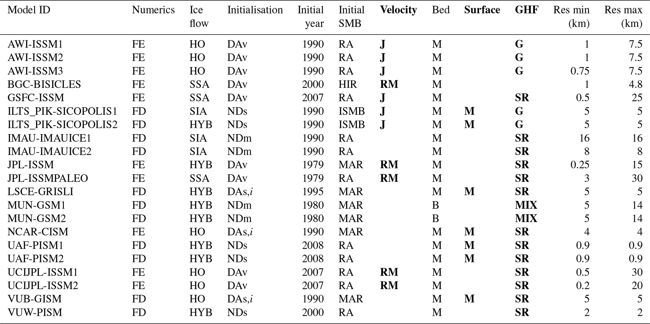
The modelling assumptions outlined in bold were not considered in the analysis, namely velocity type, surface/thickness, and geothermal heat flux (GHF) because they are not commonly shared across the different models. The reader is invited to refer to Goelzer et al. (2020) for the definition of the abbreviations for these three model characteristics.
Let us first denote sl the ith value of sea-level change calculated relative to the ith vector of p input parameters' values , where n is the total number of experiments. In the following, we present the machine learning (ML) models used in the study as well as their hyperparameters.
B1 Linear regression (LIN) model
The linear regression (LIN) model is given by
where βj denotes regression coefficients whose values are estimated using a least-squares criterion minimisation method.
B2 Random forest (RF) regression model
The random forest (RF) regression model is a non-parametric technique based on a combination (ensemble) of tree predictors (using regression trees; Breiman et al., 1984). Each tree in the ensemble (forest) is built based on the principle of recursive partitioning, which aims at finding an optimal partitioning of the input parameters' space by dividing it into L disjoint sets to have homogeneous Yi values in each set by minimising a splitting criterion (for instance based on the sum of squared errors; see Breiman et al., 1984). The minimal number of observations in each partition is termed node size (denoted ns).
The RF model, as introduced by Breiman (2001), aggregates the different regression trees as follows: (1) random bootstrap sampling from the training data and randomly selected mtry variables at each split; (2) constructing ntree trees T(α), where αt denotes the parameter vector based on which the tth tree is built; (3) aggregating the results from the prediction of each single tree to estimate the conditional mean of sl as
where E is the mathematical expectation and the weights wj are defined as
where I(A) is the indicator operator which equals 1 if A is true and 0 otherwise; Rl(x,α) is the partition of the tree model with parameter α which contains x.
The RF hyperparameters considered in the study are ns and mtry, which have been shown to have a large impact on the RF performance (Probst et al., 2019). The number of ntree was set to a large value of 2000 because of its smaller influence on the RF model performance (relative to ns and mtry).
B3 Extreme gradient boosting (XGB) regression model
Extreme gradient boosting (Friedman, 2001) is a tree ensemble method like RF model but differs regarding how trees are built (gradient boosting builds one tree at a time) and how tree-based results are combined (gradient boosting combines results during the fitting process).
Formally let us denote by the jth tree model prediction. The set of tree models are learnt by minimising the following regularised objective:
where , with T the number of leaves in the tth tree, and γ and λ are two regularisation parameters.
The first term l is a differentiable convex loss function that measures the difference between the prediction and the true value sli. The second term Ω penalises the complexity of the regression tree functions. Equation (B4) is solved through an additive training procedure by using a scalable implementation of Chen and Guestrin (2016) of tree boosting named “XGBoost”. Among the different hyperparameters of this algorithm, we focus on the following:
-
the maximum depth of the tree models, which corresponds to the number of nodes from the root down to the furthest leaf node (this hyperparameter controls the complexity of the tree model);
-
the learning rate, which is a scaling factor applied to each tree when it is added to the current approximation (a low rate value means that the trained model is more robust to overfitting but slower to compute);
-
the maximum number of iterations of the algorithm.
| Abbreviations/ | Definition |
| acronyms | |
| ANOVA | Analysis of variance |
| AOGCM | Atmosphere–ocean general circulation model |
| CTREE | Conditional inference trees |
| DAv | Data assimilation of velocity |
| GrIS | Greenland ice sheet |
| FD | Finite difference |
| FE | Finite element |
| HO | Higher order |
| ISM | Ice-sheet model |
| ISMIP6 | Ice Sheet Model Intercomparison Project for CMIP6 |
| LIN model | Linear regression model |
| MIROC5 | Model for Interdisciplinary Research on Climate – version 5 |
| MAE | Mean absolute error |
| ML model | Machine learning model |
| MME | Multi-model ensemble |
| MRAE | Mean relative absolute error |
| NDm | Nudging to ice mask |
| NDs | Nudging to surface elevation |
| RAE | Relative absolute error |
| RCM | Regional climate model |
| RCP | Representative Concentration Pathway |
| RF | Random forest |
| SAGE | Shapley Additive Global importancE |
| SHAP | SHapley Additive exPlanations |
| SIA | Shallow-ice approximation |
| SMB | Surface mass balance |
| SSA | Shallow-shelf approximation |
| XGB | Extreme gradient boosting |
The sea-level dataset is the one compiled by Edwards et al. (2021), https://raw.githubusercontent.com/tamsinedwards/emulandice/master/inst/extdata/20201106_SLE_SIMULATIONS.csv (last access: 2 June 2022), from the original data of Goelzer et al. (2020) by selecting the experiments with column names ice_source “GrIS”, region “ALL”, GCM “MIROC5”, and scenario “RCP8.5” and with prior exclusion of experiments with NaN (not a number) values of the retreat parameter. R scripts to reproduce the results of Sect. 4.3 corresponding to the three levels of analysis and, in particular, the different diagnostics for all MIROC5 RCP8.5-forced GrIS MME results (similar to Fig. 6) are provided by Rohmer (2022) at https://doi.org/10.5281/zenodo.7157302. The SHAP approach was implemented using the R package shapr (Sellereite and Jullum, 2020). The CTREE approach was implemented using the R package partykit (Hothorn and Zeileis, 2015). ML model fitting was performed using the R packages ranger (Wright and Ziegler, 2017) and xgboost (Chen et al., 2022).
JR designed the concept, set up the methods, and undertook the statistical analyses. JR and HG defined the protocol of experiments. JR, RT, GLC, HG, and GD analysed and interpreted the results. JR wrote the manuscript draft. JR, RT, GLC, HG, and GD reviewed and edited the manuscript.
The contact author has declared that none of the authors has any competing interests.
Publisher's note: Copernicus Publications remains neutral with regard to jurisdictional claims in published maps and institutional affiliations.
For the ISMIP6 results used in this study, we thank the Climate and Cryosphere (CliC) effort, which provided support for ISMIP6 through sponsoring of workshops, hosting the ISMIP6 website and wiki, and promoting ISMIP6. We acknowledge the World Climate Research Programme, which, through its Working Group on Coupled Modelling, coordinated and promoted CMIP5. We thank the climate modelling groups for producing and making available their model output, the Earth System Grid Federation (ESGF) for archiving the CMIP data and providing access, the University at Buffalo for ISMIP6 data distribution and upload, and the multiple funding agencies who support CMIP5 and ESGF. We thank the ISMIP6 steering committee, the ISMIP6 model selection group, and the ISMIP6 dataset preparation group for their continuous engagement in defining ISMIP6. This is ISMIP6 contribution no. 27. Some resources were provided by Sigma2 – the National Infrastructure for High Performance Computing and Data Storage in Norway through projects NN8006K, NN8085K, NS8006K, NS8085K, NS9560K, NS9252K, and NS5011K.
This publication was supported by PROTECT. This project has received funding from the European Union's Horizon 2020 research and innovation programme under grant agreement no. 869304, PROTECT contribution number 48. In addition, HG has received funding from the Research Council of Norway under projects 270061, 295046, and 324639.
This paper was edited by Ginny Catania and reviewed by two anonymous referees.
Aas, K., Jullum, M., and Løland, A.: Explaining individual predictions when features are dependent: More accurate approximations to Shapley values, Artif. Intell., 298, 103502, https://doi.org/10.1016/j.artint.2021.103502, 2021.
Achen, C. H.: Intepreting and Using Regression, Sage Publications, Thousand Oaks, https://doi.org/10.4135/9781412984560, 1982.
Aschwanden, A., Bartholomaus, T. C., Brinkerhoff, D. J., and Truffer, M.: Brief communication: A roadmap towards credible projections of ice sheet contribution to sea level, The Cryosphere, 15, 5705–5715, https://doi.org/10.5194/tc-15-5705-2021, 2021.
Bamber, J. L., Griggs, J. A., Hurkmans, R. T. W. L., Dowdeswell, J. A., Gogineni, S. P., Howat, I., Mouginot, J., Paden, J., Palmer, S., Rignot, E., and Steinhage, D.: A new bed elevation dataset for Greenland, The Cryosphere, 7, 499–510, https://doi.org/10.5194/tc-7-499-2013, 2013.
Barthel, A., Agosta, C., Little, C. M., Hattermann, T., Jourdain, N. C., Goelzer, H., Nowicki, S., Seroussi, H., Straneo, F., and Bracegirdle, T. J.: CMIP5 model selection for ISMIP6 ice sheet model forcing: Greenland and Antarctica, The Cryosphere, 14, 855–879, https://doi.org/10.5194/tc-14-855-2020, 2020.
Batunacun, Wieland, R., Lakes, T., and Nendel, C.: Using Shapley additive explanations to interpret extreme gradient boosting predictions of grassland degradation in Xilingol, China, Geosci. Model Dev., 14, 1493–1510, https://doi.org/10.5194/gmd-14-1493-2021, 2021.
Betancourt, C., Stomberg, T. T., Edrich, A.-K., Patnala, A., Schultz, M. G., Roscher, R., Kowalski, J., and Stadtler, S.: Global, high-resolution mapping of tropospheric ozone – explainable machine learning and impact of uncertainties, Geosci. Model Dev., 15, 4331–4354, https://doi.org/10.5194/gmd-15-4331-2022, 2022.
Breiman, L.: Random forests, Mach. Learn., 45, 5–32, 2001.
Breiman, L., Friedman, J. H., Olshen, R. A., and Stone, C. J.: Classification and regression trees, Routledge, New York, 368 pp., https://doi.org/10.1201/9781315139470, 1984.
Bussmann, N., Giudici, P., Marinelli, D., and Papenbrock, J.: Explainable machine learning in credit risk management, Comput. Econ., 57, 203–216, 2021.
Chen, T. and Guestrin, C.: Xgboost: A scalable tree boosting system, in: Proceedings of the 22nd acm sigkdd international conference on knowledge discovery and data mining, 13–17 August 2016, San Francisco, CA, USA, 785–794, https://doi.org/10.1145/2939672.2939785, 2016.
Chen, T., He, T., Benesty, M., Khotilovich, V., Tang, Y., Cho, H., Chen, K., Mitchell, R., Cano, I., Zhou, T., Li, M., Xie, J., Lin, M., Geng, Y., Li, Y., and Yuan, J.: Xgboost: extreme gradient boosting. R package version 1.6.0.1, https://cran.r-project.org/web/packages/xgboost/index.html, last access: 2 June 2022.
Covert, I., Lundberg, S. M., and Lee, S. I.: Understanding global feature contributions with additive importance measures, Adv. Neur. In., 33, 17212–17223, 2020.
Do, N. C. and Razavi, S.: Correlation effects? A major but often neglected component in sensitivity and uncertainty analysis, Water Resour. Res., 56, e2019WR025436, https://doi.org/10.1029/2019WR025436, 2020.
Edwards, T. L., Nowicki, S., Marzeion, B., Hock, R., Goelzer, H., Seroussi, H., Jourdain, N. C., Slater, D. A., Turner, F. E., Smith, C. J., McKenna, C. M., Simon, E., Abe-Ouchi, A., Gregory, J. M., Larour, E., Lipscomb, W. H., Payne, A. J., Shepherd, A., Agosta, C., Alexander, P., Albrecht, T., Anderson, B., Asay-Davis, X., Aschwanden, A., Barthel, A., Bliss, A., Calov, R., Chambers, C., Champollion, N., Choi, Y., Cullather, R., Cuzzone, J., Dumas, C., Felikson, D., Fettweis, X., Fujita, K., Galton-Fenzi, B. K., Gladstone, R., Golledge, N. R., Greve, R., Hattermann, T., Hoffman, M. J., Humbert, A., Huss, M., Huybrechts, P., Immerzeel, W., Kleiner, T., Kraaijenbrink, P., Le clec'h, S., Lee, V., Leguy, G. R., Little, C. M., Lowry, D. P., Malles, J.-H., Martin, D. F., Maussion, F., Morlighem, M., O'Neill, J. F., Nias, I., Pattyn, F., Pelle, T., Price, S. F., Quiquet, A., Radić, V., Reese, R., Rounce, D. R., Rückamp, M., Sakai, A., Shafer, C., Schlegel, N.-J., Shannon, S., Smith, R. S., Straneo, F., Sun, S., Tarasov, L., Trusel, L. D. Van Breedam, J., van de Wal, R., van den Broeke, M., Winkelmann, R., Zekollari, H., Zhao, C., Zhang, T., and Zwinger, T.: Projected land ice contributions to twenty-first-century sea level rise, Nature, 593, 74-82, 2021.
Evin, G., Hingray, B., Blanchet, J., Eckert, N., Morin, S., and Verfaillie, D.: Partitioning uncertainty components of an incomplete ensemble of climate projections using data augmentation, J. Climate, 32, 2423–2440, 2019.
Fisher, A., Rudin, C., and Dominici, F.: All Models are Wrong, but Many are Useful: Learning a Variable's Importance by Studying an Entire Class of Prediction Models Simultaneously, J. Mach. Learn. Res., 20, 1–81, 2019.
Frye, C., de Mijolla, D., Cowton, L., Stanley, M., and Feige, I.: Shapley-based explainability on the data manifold, arXiv [preprint], https://doi.org/10.48550/arXiv.2006.01272, 2020.
Friedman, J.: Greedy function approximation: a gradient boosting machine, Ann. Stat., 29, 1189–1232, 2001.
Grinsztajn, L., Oyallon, E., and Varoquaux, G.: Why do tree-based models still outperform deep learning on tabular data?, arXiv [preprint], https://doi.org/10.48550/arXiv.2207.08815, 2022.
Goelzer, H., Nowicki, S., Edwards, T., Beckley, M., Abe-Ouchi, A., Aschwanden, A., Calov, R., Gagliardini, O., Gillet-Chaulet, F., Golledge, N. R., Gregory, J., Greve, R., Humbert, A., Huybrechts, P., Kennedy, J. H., Larour, E., Lipscomb, W. H., Le clec'h, S., Lee, V., Morlighem, M., Pattyn, F., Payne, A. J., Rodehacke, C., Rückamp, M., Saito, F., Schlegel, N., Seroussi, H., Shepherd, A., Sun, S., van de Wal, R., and Ziemen, F. A.: Design and results of the ice sheet model initialisation experiments initMIP-Greenland: an ISMIP6 intercomparison, The Cryosphere, 12, 1433–1460, https://doi.org/10.5194/tc-12-1433-2018, 2018.
Goelzer, H., Nowicki, S., Payne, A., Larour, E., Seroussi, H., Lipscomb, W. H., Gregory, J., Abe-Ouchi, A., Shepherd, A., Simon, E., Agosta, C., Alexander, P., Aschwanden, A., Barthel, A., Calov, R., Chambers, C., Choi, Y., Cuzzone, J., Dumas, C., Edwards, T., Felikson, D., Fettweis, X., Golledge, N. R., Greve, R., Humbert, A., Huybrechts, P., Le clec'h, S., Lee, V., Leguy, G., Little, C., Lowry, D. P., Morlighem, M., Nias, I., Quiquet, A., Rückamp, M., Schlegel, N.-J., Slater, D. A., Smith, R. S., Straneo, F., Tarasov, L., van de Wal, R., and van den Broeke, M.: The future sea-level contribution of the Greenland ice sheet: a multi-model ensemble study of ISMIP6, The Cryosphere, 14, 3071–3096, https://doi.org/10.5194/tc-14-3071-2020, 2020.
Hastie, T., Tibshirani, R., and Friedman, J.: The Elements of Statistical Learning: Data Mining, Inference, and Prediction, Springer, Berlin/Heidelberg, Germany, ISSN 0172-7397, 2009.
Hawkins, E. and Sutton, R.: The potential to narrow uncertainty in regional climate predictions, B. Am. Meteorol. Soc., 90, 1095–1107, 2009.
Hothorn, T. and Zeileis, A.: partykit: A modular toolkit for recursive partytioning in R, J. Mach. Learn. Res., 16, 3905–3909, 2015.
Hothorn, T., Hornik, K., and Zeileis, A.: Unbiased Recursive Partitioning: A Conditional Inference Framework, J. Comput. Graph. Stat., 15, 651–74, 2006.
Iooss, B. and Prieur, C.: Shapley effects for sensitivity analysis with correlated inputs: comparisons with Sobol' indices, numerical estimation and applications, Int. J. Uncertain. Quan., 9, 493–514, https://doi.org/10.1615/Int.J.UncertaintyQuantification.2019028372, 2019.
Jack, C. D., Jones, R., Burgin, L., and Daron, J.: Climate risk narratives: An iterative reflective process for co-producing and integrating climate knowledge, Climate Risk Management, 29, 100239, https://doi.org/10.1016/j.crm.2020.100239, 2020.
Jothi, N. and Husain, W.: Predicting generalized anxiety disorder among women using Shapley value, J. Infect. Public Heal., 14, 103–108, 2021.
Kaur, H., Nori, H., Jenkins, S., Caruana, R., Wallach, H., and Wortman Vaughan, J.: Interpreting interpretability: understanding data scientists' use of interpretability tools for machine learning, in: Proceedings of the 2020 CHI conference on human factors in computing systems, 25–30 April 2020, Honolulu, HI, USA, 1–14, https://doi.org/10.1145/3313831.3376219, 2020.
Kopp, R. E., Gilmore, E. A., Little, C. M., Lorenzo-Trueba, J., Ramenzoni, V. C., and Sweet, W. V.: Usable science for managing the risks of sea-level rise, Earth's Future, 7, 1235–1269, 2019.
Lundberg, S. M. and Lee, S. I.: A unified approach to interpreting model predictions, in: Proceedings of the 31st international conference on neural information processing systems, 4–9 December 2017, Long Beach, CA, USA, 4768–4777, https://doi.org/10.5555/3295222.3295230, 2017.
Lundberg, S. M., Erion, G., Chen, H., DeGrave, A., Prutkin, J. M., Nair, B., Katz, R., Himmelfarb, J., Bansal, N., and Lee; S.-I.: From local explanations to global understanding with explainable AI for trees, Nature Machine Intelligence, 2, 56–67, 2020.
Molnar, C., Casalicchio, G., and Bischl, B.: Interpretable machine learning – a brief history, state-of-the-art and challenges, in: Joint European Conference on Machine Learning and Knowledge Discovery in Databases, Springer, Cham, 14–18 September 2020, Ghent, Belgium, https://doi.org/10.1007/978-3-030-65965-3_28417--431, 2020.
Molnar, C.: Interpretable Machine Learning: A Guide for Making Black Box Models Explainable, 2nd Edn., http://christophm.github.io/interpretable-ml-book/, ast access: 2 June 2022.
Morlighem, M., Williams, C. N., Rignot, E., An, L., Arndt, J. E., Bamber, J. L., Catania, G., Chauché, N., Dowdeswell, J. A., Dorschel, B., Fenty, I., Hogan, K., Howat, I., Hubbard, A., Jakobsson, M., Jordan, T. M., Kjeldsen, K. K., Millan, R., Mayer, L., Mouginot, J., Noël, B. P. Y., O'Cofaigh, C., Palmer, S., Rysgaard, S., Seroussi, H., Siegert, M. J., Slabon, P., Straneo, F., van den Broeke, M. R., Weinrebe, W., Wood, M., and Zinglersen, K. B.: BedMachine v3: Complete bed topography and ocean bathymetry mapping of Greenland from multi-beam radar sounding combined with mass conservation. Geophys. Res. Lett., 44, 11051–11061, https://doi.org/10.1002/2017GL074954, 2017.
Murdoch, W. J., Singh, C., Kumbier, K., Abbasi-Asl, R., and Yu, B.: Definitions, methods, and applications in interpretable machine learning, P. Natl. Acad. Sci. USA, 116, 22071–22080, 2019.
Murphy, J. M., Sexton, D. M., Barnett, D. N., Jones, G. S., Webb, M. J., Collins, M., and Stainforth, D. A.: Quantification of modelling uncertainties in a large ensemble of climate change simulations, Nature, 430, 768–772, 2004.
Northrop, P. J. and Chandler, R. E.: Quantifying sources of uncertainty in projections of future climate, J. Climate, 27, 8793–8808, 2014.
Nowicki, S. M. J., Payne, A., Larour, E., Seroussi, H., Goelzer, H., Lipscomb, W., Gregory, J., Abe-Ouchi, A., and Shepherd, A.: Ice Sheet Model Intercomparison Project (ISMIP6) contribution to CMIP6, Geosci. Model Dev., 9, 4521–4545, https://doi.org/10.5194/gmd-9-4521-2016, 2016.
Nowicki, S., Goelzer, H., Seroussi, H., Payne, A. J., Lipscomb, W. H., Abe-Ouchi, A., Agosta, C., Alexander, P., Asay-Davis, X. S., Barthel, A., Bracegirdle, T. J., Cullather, R., Felikson, D., Fettweis, X., Gregory, J. M., Hattermann, T., Jourdain, N. C., Kuipers Munneke, P., Larour, E., Little, C. M., Morlighem, M., Nias, I., Shepherd, A., Simon, E., Slater, D., Smith, R. S., Straneo, F., Trusel, L. D., van den Broeke, M. R., and van de Wal, R.: Experimental protocol for sea level projections from ISMIP6 stand-alone ice sheet models, The Cryosphere, 14, 2331–2368, https://doi.org/10.5194/tc-14-2331-2020, 2020.
Padarian, J., McBratney, A. B., and Minasny, B.: Game theory interpretation of digital soil mapping convolutional neural networks, SOIL, 6, 389–397, https://doi.org/10.5194/soil-6-389-2020, 2020.
Probst, P., Wright, M. N., and Boulesteix, A. L.: Hyperparameters and tuning strategies for random forest, Wires Data Min. Knowl., 9, e1301, https://doi.org/10.1002/widm.1301, 2019.
Razavi, S., Jakeman, A., Saltelli, A., Prieur, C., Iooss, B., Borgonovo, E., Plischke, E., Lo Piano, S., Iwanaga, T., Becker, W., Tarantola, S., Guillaume, J. H. A., Jakeman, J., Gupta, H., Melillo, N., Rabitti, G., Chabridon, V., Duan, Q., Sun, X., Smith, S., Sheikholeslami, R., Hosseini, N., Asadzadeh, M., Puy, A., Kucherenko, S., Maier, H. R.: The future of sensitivity analysis: an essential discipline for systems modeling and policy support, Environ. Model. Softw., 137, 104954, https://doi.org/10.1016/j.envsoft.2020.104954, 2021.
Redelmeier, A., Jullum, M., and Aas, K.: Explaining Predictive Models with Mixed Features Using Shapley Values and Conditional Inference Trees, in: Machine Learning and Knowledge Extraction, edited by: Holzinger, A., Kieseberg, P., Tjoa, A., and Weippl, E., CD-MAKE 2020, Lecture Notes in Computer Science, Springer Cham., 12279, 117–137, https://doi.org/10.1007/978-3-030-57321-8_7, 2020.
Rohmer, J.: Local explanation SHAP approach applied to MIROC5,RCP8.5-forced multi-model ensemble study of GrIS future sea-level contributions, Zenodo [data set and code], https://doi.org/10.5281/zenodo.7157302, 2022.
Shrestha, N.: Detecting multicollinearity in regression analysis, Am. J. Appl. Math. Stat., 8, 39–42, 2020.
Sellereite, N. and Jullum, M.: shapr: An R-package for explaining machine learning models with dependence-aware Shapley values, J. Open Source Softw., 5, 2027, https://doi.org/10.21105/joss.02027, 2020.
Seroussi, H., Nowicki, S., Payne, A. J., Goelzer, H., Lipscomb, W. H., Abe-Ouchi, A., Agosta, C., Albrecht, T., Asay-Davis, X., Barthel, A., Calov, R., Cullather, R., Dumas, C., Galton-Fenzi, B. K., Gladstone, R., Golledge, N. R., Gregory, J. M., Greve, R., Hattermann, T., Hoffman, M. J., Humbert, A., Huybrechts, P., Jourdain, N. C., Kleiner, T., Larour, E., Leguy, G. R., Lowry, D. P., Little, C. M., Morlighem, M., Pattyn, F., Pelle, T., Price, S. F., Quiquet, A., Reese, R., Schlegel, N.-J., Shepherd, A., Simon, E., Smith, R. S., Straneo, F., Sun, S., Trusel, L. D., Van Breedam, J., van de Wal, R. S. W., Winkelmann, R., Zhao, C., Zhang, T., and Zwinger, T.: ISMIP6 Antarctica: a multi-model ensemble of the Antarctic ice sheet evolution over the 21st century, The Cryosphere, 14, 3033–3070, https://doi.org/10.5194/tc-14-3033-2020, 2020.
Shapley, L. S.: A value for n-person games, in: Contributions to the Theory of Games, Volume II, Annals of Mathematics Studies, edited by: Kuhn, H. and Tucker, A. W., Princeton University Press, Princeton, NJ, chap. 17, 307–317, https://doi.org/10.1515/9781400881970-018, 1953.
Slater, D. A., Straneo, F., Felikson, D., Little, C. M., Goelzer, H., Fettweis, X., and Holte, J.: Estimating Greenland tidewater glacier retreat driven by submarine melting, The Cryosphere, 13, 2489–2509, https://doi.org/10.5194/tc-13-2489-2019, 2019.
Slater, D. A., Felikson, D., Straneo, F., Goelzer, H., Little, C. M., Morlighem, M., Fettweis, X., and Nowicki, S.: Twenty-first century ocean forcing of the Greenland ice sheet for modelling of sea level contribution , The Cryosphere, 14, 985–1008, https://doi.org/10.5194/tc-14-985-2020, 2020.
Stammer, D., Van de Wal, R. S. W., Nicholls, R. J., Church, J. A., Le Cozannet, G., Lowe, J. A., Horton, B. P., White, K., Behar, D., and Hinkel, J.: Framework for high-end estimates of sea level rise for stakeholder applications, Earth's Future, 7, 923–938, 2019.
Štrumbelj, E. and Kononenko, I.: Explaining prediction models and individual predictions with feature contributions, Knowl. Inf. Syst., 41, 647–665, 2014.
van der Laan, M. J., Polley, E. C., and Hubbard, A. E.: Super learner, Statistical applications in genetics and molecular biology, 6, 1–23, https://doi.org/10.2202/1544-6115.1309, 2007.
Wright, M. N. and Ziegler, A.: ranger: A Fast Implementation of Random Forests for High Dimensional Data in C and R, J. Stat. Softw., 77, 1–17, 2017.
Yip, S., Ferro, C. A., Stephenson, D. B., and Hawkins, E.: A simple, coherent framework for partitioning uncertainty in climate predictions, J. Climate, 24, 4634–4643, 2011.
- Abstract
- Introduction
- Multi-model ensemble case study
- Methods
- Application
- Discussion
- Concluding remarks and further work
- Appendix A: Model characteristics
- Appendix B: ML models and hyperparameters' definition
- Appendix C: List of abbreviations/acronyms
- Code and data availability
- Author contributions
- Competing interests
- Disclaimer
- Acknowledgements
- Financial support
- Review statement
- References
SHapley Additive exPlanationsapproach to a subset of a multi-model ensemble study for the Greenland ice sheet. This allows us to quantify the influence of particular modelling decisions (related to numerical implementation, initial conditions, or parametrisation of ice-sheet processes) directly in terms of sea-level change contribution.
- Abstract
- Introduction
- Multi-model ensemble case study
- Methods
- Application
- Discussion
- Concluding remarks and further work
- Appendix A: Model characteristics
- Appendix B: ML models and hyperparameters' definition
- Appendix C: List of abbreviations/acronyms
- Code and data availability
- Author contributions
- Competing interests
- Disclaimer
- Acknowledgements
- Financial support
- Review statement
- References