Exploring the capabilities of electrical resistivity tomography to study subsea permafrost

Sea level rise and coastal erosion have inundated large areas of Arctic permafrost. Submergence by warm and saline waters increases the rate of inundated permafrost thaw compared to sub-aerial thawing on land. Studying the contact between the unfrozen and frozen sediments below the seabed, also known as the ice-bearing permafrost table (IBPT), provides valuable information to understand the evolution of sub-aquatic permafrost, which is key to improving and understanding coastal erosion prediction models and potential greenhouse gas emissions. In this study, we use data from 2D electrical resistivity tomography (ERT) collected in the nearshore coastal zone of two Arctic regions that differ in their environmental conditions (e.g., seawater depth and resistivity) to image and study the subsea permafrost. The inversion of 2D ERT data sets is commonly performed using deterministic approaches that favor smoothed solutions, which are typically interpreted using a user-specified resistivity threshold to identify the IBPT position. In contrast, to target the IBPT position directly during inversion, we use a layer-based model parameterization and a global optimization approach to invert our ERT data. This approach results in ensembles of layered 2D model solutions, which we use to identify the IBPT and estimate the resistivity of the unfrozen and frozen sediments, including estimates of uncertainties. Additionally, we globally invert 1D synthetic resistivity data and perform sensitivity analyses to study, in a simpler way, the correlations and influences of our model parameters. The set of methods provided in this study may help to further exploit ERT data collected in such permafrost environments as well as for the design of future field experiments.

1 Introduction

In Arctic coastal regions, contemporary subsea permafrost thawing starts following the inundation caused by sea level rise and coastal erosion. Seawater is typically warmer than mean annual air temperatures, and the presence of saltwater (mostly through diffusive processes) lowers the freezing point of the seabed (Harrison and Osterkamp, 1978; Are, 2003). Additionally, groundwater flow of freshwater from inland areas might play an important role in thawing permafrost (Frederick and Buffett, 2015; Pedrazas et al., 2020), comparable to warm discharge from large rivers (Shakhova et al., 2017). Subsea permafrost is estimated to contain a large quantity of organic carbon (Sayedi et al., 2020), which can decompose microbially to generate carbon dioxide and/or methane after the permafrost thaws. Furthermore, gas hydrates are present in subsea permafrost and may act as an additional source of methane if they dissociate (Ruppel and Kessler, 2017). Understanding the development of permafrost degradation rates helps to fine-tune predictive models of greenhouse gas emissions that may represent a positive feedback for climate warming (Schuur et al., 2015). Furthermore, the correlation between permafrost degradation and coastal erosion proposed by Are (2003) and Overduin et al. (2012, 2016) might be used to refine coastal dynamics models.

Subsea permafrost is a perennially cryotic (<0 ^∘C) layer or body of sediments underneath a marine water column (Angelopoulos et al., 2020a). These sediments can be frozen or unfrozen. A layer of unfrozen ground in a permafrost area is known as talik, and in particular, the perennially cryotic unfrozen sediments forming part of the permafrost are known as cryopegs (Permafrost Subcommittee, 1988). Cryopegs can be isolated pockets or layers and are commonly found along Arctic coasts in saline marine sediments that are exposed following a marine regression, for example, due to isostatic uplift (O'Neill et al., 2020). Offshore, cryotic unfrozen sediment in between the water column and frozen ground is still generally referred to as a talik (Osterkamp, 2001). The subsea permafrost that contains ice is known as ice-bearing permafrost, and when the soil particles are cemented together by ice, it is termed ice-bonded permafrost (Permafrost Subcommittee, 1988). Because traditional geophysical methods such as electrical resistivity tomography (ERT) and seismic techniques can only distinguish between sediments with no or low ice content from those with high ice content (note that direct sampling is required for a quantitative estimation of ice content), we refer to them as unfrozen and frozen sediments in this study, and the interface that separates them is the ice-bearing permafrost table (IBPT). Imaging and determining the position of the IBPT (e.g., using geophysical or borehole data) is important for a better process understanding of subsea permafrost evolution and to infer degradation rates. For example, dividing the depth to the IBPT by the time since inundation results in the mean annual degradation rate (e.g., Are, 2003; Overduin et al., 2012, 2016).

Among the most used geophysical imaging techniques to study the subsea permafrost are different electromagnetic and seismic methods as well as ERT (Scott et al., 1990; Kneisel et al., 2008; Hubbard et al., 2013). Electromagnetic induction (EMI) methods are promising techniques to map both the top and bottom boundaries of the permafrost and might be used for a wide range of water depths (e.g., Sherman et al., 2017). EMI methods can properly work under low-resistivity seawater layers, while the use of ground-penetrating radar (GPR) is limited to freshwater bottom-fast ice environments characterized by high electrical resistivity values as found in delta areas (e.g., Stevens et al., 2009). Seismic methods have been employed widely in deep-water environments (e.g., Rekant et al., 2015; Brothers et al., 2016), and, more recently, researchers have used recordings of ambient seismic noise in shallow waters to map the IBPT (e.g., Overduin et al., 2015a). The ERT method is a suitable tool to investigate the resistivity distribution of the unfrozen sediments (e.g., talik and cryopeg) and for studying and delineating the IBPT position (e.g., Sellmann et al., 1989; Overduin et al., 2012, 2016; Angelopoulos et al., 2019, 2020b; Angelopoulos, 2022; Pedrazas et al., 2020).

In marine ERT surveying, floating electrodes are typically used to inject a current and measure potential differences that are used to calculate apparent electrical resistivity data. In the summer season of the Arctic, the measured values are often influenced by the resistivity and thickness of the water layer and by the unfrozen and frozen sediments. The ERT method can detect the IBPT but does not necessarily distinguish non-cryotic from cryotic taliks above the IBPT. The resistivity of seawater depends mainly on the amount of dissolved salts and temperature. The dissolved salts are mostly affected by water inflows from rivers and the cycles of sea ice melting, freezing, and brine release. The resistivity of the seawater is commonly in the range of 0.1 to 40 Ω m (e.g., Sellmann et al., 1989; Lantuit et al., 2011). On the other hand, the resistivity of the underlying sediments is influenced by porosity, pore size, grain size, water and ice content, porewater salinity, and temperature (Kneisel et al., 2008; Wu et al., 2017). For example, the resistivity of unfrozen sediments typically ranges from 1 to 25 Ω m (e.g., Sellmann et al., 1989; Overduin et al., 2012; Angelopoulos et al., 2019), while the resistivities of frozen sediments might vary from 10 Ω m up to more than 1000 Ω m (e.g., Overduin et al., 2012, 2016; Pedrazas et al., 2020; Rangel et al., 2021). The higher the ice content is, the more resistive the medium is (Pearson et al., 1986; Fortier et al., 1994; Kang and Lee, 2015). In cases where the resistivity of the frozen sediments is several orders of magnitude higher than the resistivity of the overlying unfrozen sediments, the electrical current injected through the electrodes is expected to be channeled through the less resistive layers (e.g., Spitzer, 1998), resulting in a limited penetration of the current system into the frozen sediment layers.

When analyzing ERT data collected in subsea permafrost environments, defining an appropriate inversion and model parameterization strategy is critical for deriving reliable resistivity models and interpreting these models in terms of the IBPT position. For example, when a priori information suggests that the nature of the contact between the unfrozen and frozen sediments is gradual, a grid-based model parameterization and a local inversion algorithm favoring vertical and/or horizontal smoothness in the final models might be an appropriate choice (e.g., Loke and Barker, 1996; Günther et al., 2006). Here, the experience of the interpreter might help to guess a specific resistivity threshold value to define the IBPT position (e.g., Overduin et al., 2016; Sherman et al., 2017; Angelopoulos et al., 2021). Additionally, one may also consider different gradient-based image-processing approaches to extract interfaces from the inverted resistivity model (e.g., Hsu et al., 2010; Chambers et al., 2012). Finally, when we have ample evidence of a sharp contact between the unfrozen and frozen sediments (e.g., Overduin et al., 2015b; Angelopoulos et al., 2020a), a layer-based model parameterization combined with a local and/or global inversion algorithms might be more suitable (e.g., Auken and Christiansen, 2004; Akça and Basokur, 2010; De Pasquale et al., 2019; Arboleda-Zapata et al., 2022).

In this study, we adapt the inversion and ensemble interpretation strategies as proposed by Arboleda-Zapata et al. (2022) to study submarine permafrost environments of the Arctic in terms of the resistivity distribution of the unfrozen and frozen sediments and the position of the IBPT, including estimates of uncertainties. We analyze and compare ERT data collected at two field sites in the Arctic characterized by different environmental conditions regarding seawater depth and resistivity, coastal erosion rate, and the sediment porewater chemistry. Additionally, we generate and interpret ensembles of globally inverted 1D electrical data to get a deeper understanding of the inverse problem for typical resistivity distributions in these kinds of environments. Finally, we also implement local and global sensitivity analyses to recognize the most influential parameters during 2D and 1D inversions.

2 Study sites

Our field data were collected at two field sites: one offshore of the southern part of the Bykovsky Peninsula in the Siberian Laptev Sea (Fig. 1a) and the other one offshore of Drew Point in the Alaskan Beaufort Sea (Fig. 1d). To relate these data sets to the site-specific environmental settings, we summarize the main characteristics of each study area in a regional framework.

2.1 Regional setting of Bykovsky Peninsula

The Bykovsky Peninsula is located in northeastern Siberia in the vicinity of the Lena River Delta. The peninsula is mainly characterized by the presence of ice-rich sediments (volumetric ice content exceeding 80 %, also known as the Yedoma Ice Complex) that accumulated during the Late Pleistocene (Schirrmeister et al., 2002; Grosse et al., 2007). The Yedoma deposits extend to 15 m below sea level (Grigoriev, 2008). The sediments at or below sea level are composed of silt, sand, and gravel with variable grain size distributions (Grosse et al., 2007). During the Early to Middle Holocene, a general landscape transformation started, resulting in a thermokarst-dominated relief characterized by thermo-erosional valleys and thermokarst lakes (Schirrmeister et al., 2002; Grosse et al., 2007). The mean coastal erosion rates at different locations of the peninsula typically range between 0.4 and 1.5 m yr⁻¹, with maximum values of up to 10 m yr⁻¹ mainly caused by storms and thermomechanical erosion of ice-rich sediments (Lantuit et al., 2011). The seawater around the peninsula is strongly influenced by freshwater and sediments originating from the Lena River (Lantuit et al., 2011). Additionally, the resistivity of the seawater is influenced by seasonal sea ice freezing and melting as shown by Lantuit et al. (2011), who report resistivity values for the eastern shore of the Bykovsky Peninsula of less than 1 Ω m in winter and above 10 Ω m in summer. Similar water resistivity values are also reported by Overduin et al. (2016) for the seawater near Muostakh Island. The depth of the seawater for the southern part of the Bykovsky Peninsula deepens 2 m within a distance of 100 m from the shoreline and increases to 5 m at about 2000 m from the coast (Lantuit et al., 2011; Fuchs et al., 2021).

2.2 Regional setting of Drew Point

Drew Point is located on the coast of the Alaskan Beaufort Sea. The local geology is characterized by glaciomarine, fine-grained, ice-rich sediments deposited in the Late Pleistocene (Black, 1964; Ping et al., 2011). The inland geomorphology is characterized by 3–5 m high coastal bluffs, thermokarst channels and lakes, and ice-wedge polygons on tundra plains with maximum elevations of ∼10 m (Barnhart et al., 2014; Jones et al., 2018). The average coastal erosion rate between 1979 and 2002 was around 9 m yr⁻¹ (Jones et al., 2009) and increased for the period 2002 to 2016 up to approximately 20 m yr⁻¹ (Jones et al., 2018). Lück (2020) reports brackish water resistivities observed during fieldwork in July 2018 of 0.4–0.5 Ω m, with weak stratification visible in the water column profiles. The depth of the seawater offshore of Drew Point deepens to 2 m within a distance of 500 m from the shoreline and increases to 3 m at distances of about 2000 m from the coast (Jones et al., 2018).

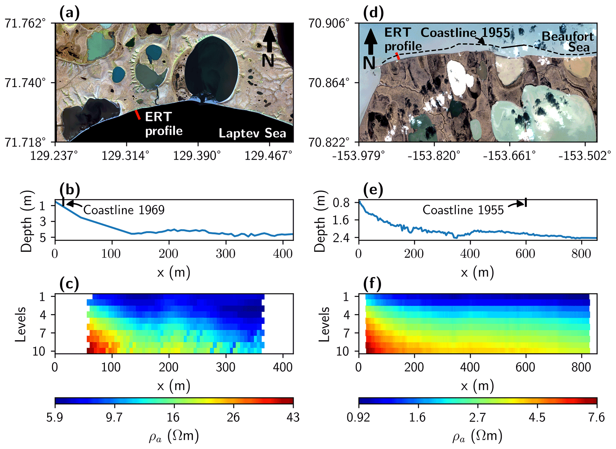
Figure 1 Location and ERT data of our field studies. (a) Bykovsky field site located at the coast of the Laptev Sea in northern Siberia (Sakha Republic, Russian Federation) and (d) Drew Point field site located at the coast of the Beaufort Sea in northern Alaska (AK, USA), where the red lines indicate ERT profile locations and the black dashed line in panel (d) indicates the position of the 1955 coastline for Drew Point (Jones et al., 2008). (b) The recorded bathymetric profile along the ERT profile for Bykovsky and (e) for Drew Point indicating the 1969 (Schirrmeister et al., 2018) and 1955 coastline positions, respectively. The current coast position for both profiles is at $x\approx -\mathrm{10}$ m. (c) Pseudosection of the recorded raw ERT data for Bykovsky and (f) for Drew Point. Bykovsky satellite image: WorldView-3 satellite product from 2 September 2016; © Digital Globe. Drew Point satellite image: Planet satellite image from 3 September 2017.

3 Data acquisition

In marine ERT data acquisition, there is typically an excellent coupling between the floating electrodes and the seawater. This allows us to perform voltage measurements while the boat pulling the electrode streamer is in motion (preferably at constant speed) and, thus, to also efficiently measure profiles with a length on the order of kilometers. The sources of errors during data acquisition are mainly related to misalignments of the electrode streamer (e.g., due to water currents), the precision of electrode positioning (which is given relative to boat position), vertical oscillation of electrodes (e.g., due to wavy conditions), and surface area limitation of injection voltage. Furthermore, due to the large variety of environmental settings, one must tailor the survey parameters to each field site, which includes varying the electrode spacing, the transmitter voltage, the measurement duration, the boat speed, the digital resolution of the potential measurements, and the sampling frequency.

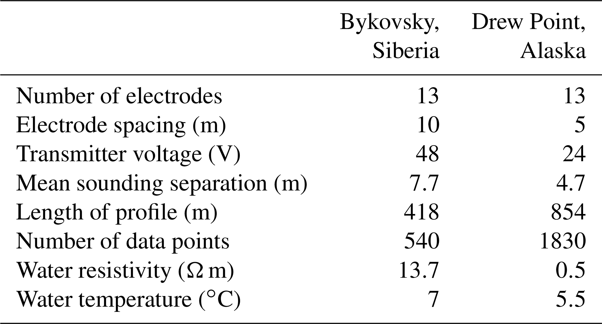
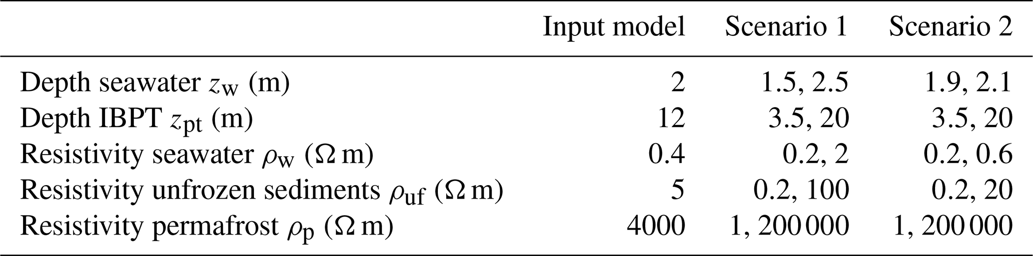
In Table 1, we compare the acquisition parameters for our ERT data from Bykovsky and Drew Point, which were collected during two fieldwork campaigns in July 2017 and July 2018, respectively. The two ERT data sets were collected using an Iris™ Syscal Pro Deep Marine system employing a streamer cable with 13 equally spaced floating electrodes. The resistivity measurements were acquired using a reciprocal Wenner–Schlumberger array configuration, where current was injected through the inner pair of electrodes and quasi-symmetric voltages were measured simultaneously with 10 channels using the outer pairs of electrodes (e.g., Overduin et al., 2012). The transmitter voltage was set at approximately 48 V at Bykovsky, while at Drew Point it was reduced to 24 V to avoid exceeding the electrode surface area limits. Additionally, different electrode spacings were used. The Bykovsky data were recorded using a 10 m spacing between electrodes, while at Drew Point 5 m spacing was chosen because the rapid coastal erosion rates suggested that the IBPT position at this field site should be shallower than at our Siberian field site for a given distance offshore. To collect the data along every profile, a cable was towed behind a small inflatable boat and voltages were measured as the boat moved at approximately constant speed of ∼1 m s⁻¹ perpendicular to the shore. The Bykovsky soundings were collected at spacings of ∼7.7 m along a 418 m long profile, resulting in 540 measurements. At Drew Point, the soundings were collected at spacings of ∼4.7 m along a 854 m long profile, resulting in 1830 measurements. At both field sites, the electrode positions were estimated relative to the position of a GPS aboard the boat assuming a straight streamer cable. Complementary to the ERT measurements, we also recorded the water depth at each sounding location using a Garmin echo sounder attached to the boat (Fig. 1b, and e). Furthermore, we measured during each field campaign water resistivity and temperature at different depths close to our ERT profiles (the mean values are shown in the last two rows of Table 1) using a SonTek™ CastAway device also known as CTD. In general, at our Drew Point field site, the seawater was shallower, less resistive, and slightly cooler than at our Bykovsky field site. Furthermore, the CTD measurements suggest low vertical and horizontal variations in the resistivity of the water layer at both field sites. For example, the largest variations are in the horizontal direction and are on the order of 1 and 0.04 Ω m for our Bykovsky and Drew Point data sets, respectively.

Table 1 Acquisition parameters for our ERT data sets and further site-specific information for our two field sites.

The measured apparent resistivities ρ_a are presented as pseudosections in Fig. 1c and f. Here the x coordinates represent the center position of each quadripole, and the vertical axes represent the relative penetration also known as levels; i.e., level =1 is the shortest quadripole, while level =10 is the quadripole with maximum electrode spacing. The range of ρ_a for Bykovsky is 5.9 to 43 Ω m and for Drew Point 0.9 to 7.6 Ω m. The lower ρ_a values at Drew Point are mainly due to the lower resistivity of the seawater at the Alaskan coast, which is less influenced by freshwater discharge from large rivers than at our Bykovsky field site. Additionally, we notice that levels larger than seven in our Bykovsky data set are characterized by higher variations due to noise or 3D subsurface structures. In contrast, the Drew Point data do not show obvious variations depending on the level number.

4 Methodology

In this study, we follow the workflow of Arboleda-Zapata et al. (2022), who propose a layer-based model parameterization to globally invert 2D ERT data, which is used to generate an ensemble of representative model solutions. For completeness, we present a brief summary of this workflow in the following. For a more detailed analysis, we will also address complementary strategies such as 1D inversion tests as well as local and global sensitivity analyses.

4.1 Two-dimensional layer-based model parameterization

One of the most important steps in any geophysical inversion workflow is defining a model parameterization that can properly represent the studied geological environment. Because a priori information suggests a layered subsurface (i.e., unfrozen sediments overlying frozen sediments) at both of our field sites, we choose a layer-based model parameterization considering an unstructured mesh with local refinements along the interfaces separating individual layers. Additionally, because resistivity variations within each layer are negligible compared to the variations between different layers, we assume homogeneous layers; i.e., each layer is characterized by one resistivity value. For more complex geological settings, one might allow for lateral and/or vertical variations within the layers (e.g., Auken and Christiansen, 2004; Akça and Basokur, 2010). To parameterize the interface geometry that defines the contact between the individual layers, we may use different strategies, for example, based on spline interpolation (e.g., Koren et al., 1991), Fourier coefficients (e.g., Roy et al., 2021), or sums of arctangent functions (Gebrande, 1976).

Allowing for abrupt changes along the interfaces is considered to be a critical point in subsea permafrost environments where high structural variability is often found. In such environments, we expect sharp boundaries and variations along the interfaces due to inundated thermokarst structures (Angelopoulos et al., 2021), pingo-like features, bottom-fast ice versus floating ice regime transitions in winter, or changes in the ratio of coastal erosion vs. degradation rate; i.e., changing from a period of fast thawing and low coastal erosion to a period of fast coastal erosion and slow thawing can result in a heterogeneous structure of the IBPT (e.g., Overduin et al., 2016). Because we expect some of these processes and structures at our field sites, we adopt a strategy based on the sums of arctangent functions because it allows for abrupt and smooth changes along the interfaces (e.g., Roy et al., 2005; Rumpf and Tronicke, 2015). Following Arboleda-Zapata et al. (2022), the sums of arctangent functions for a single interface can be written as

$$\begin{array}{}\text{(1)}& z\left(x\right)=z_{\mathrm{0}}+\sum _{j=\mathrm{0}}^{n_{\mathrm{nod}}}\mathrm{\Delta }{z}_j\left(\mathrm{0.5}+{\displaystyle \frac{\mathrm{1}}{\mathit{\pi }}}{\tan }^{-\mathrm{1}}\left(x-{\displaystyle \frac{x_j}{b_j}}\right)\right),\end{array}$$

where z is the depth, n_nod is the number of arctangent nodes, z₀ is the average depth of the interface, x_j is the horizontal location of an arctangent node, and Δz_j is the vertical throw attained asymptotically over a horizontal distance of b_j. Such sets of coefficients are used to obtain z(x) at horizontal distances x. Increasing the number of nodes allows us to resolve more complex interfaces. During preliminary experiments and parameter testing, we noticed that using three to seven nodes allows us to model rather complex interfaces. For both of our field studies, we fix the number of nodes to five, which results in 16 model parameters (1+3n_nod) per interface. Because we consider two interfaces, one for the seabed and the other for the IBPT separating three layers with homogeneous resistivities, our parameterization strategy results in a total of 35 model parameters.

4.2 Inversion strategy

During inversion, we search for a combination of model parameters (i.e., those describing the geometry of interfaces using Eq. 1 and the resistivities of the homogeneous layers) that minimizes the root mean squared logarithmic error (RMSLE). To reduce the space of possible solutions, we consider some constraints in our layer-based parameterization approach. For both case studies, we constrain the seabed position (Fig. 1b and e) allowing vertical variations of up to ±0.15 m, which is the approximate error level of our echo sounder data for water depths <5 m. Considering our CTD measurements, we allow the resistivity of the water to vary between 11 and 15 Ω m for our Bykovsky data and between 0.2 and 2 Ω m for our Drew Point data. Note that we consider additional freedom beyond the variabilities reported in Sect. 3 (1 Ω m for Bykovsky and 0.04 Ω m for Drew Point) to account for additional variations related to the different sensitivities and resolutions of our CTD and ERT data. Additionally, we set our search parameter range for the resistivity of the talik from 1 to 100 Ω m and that for the resistivity of the ice-bearing permafrost from 1 to 300 000 Ω m for both field studies.

Because we aim to find an inverse model independent of a reference or starting model, we use a global inversion strategy based on the particle swarm optimization (PSO) technique, which was originally introduced by Kennedy and Eberhart (1995). Over the last decade, the PSO algorithm has been widely used to invert different types of geophysical data sets because it has proven to be an effective tool for finding different local minima in objective functions with complicated topography (e.g., Tronicke et al., 2012; Fernández-Martínez et al., 2017).

In a first step, the PSO requires defining a set of particles where each particle represents a different model. The particles are initialized with random parameters bounded within realistic physical ranges. This defines our model space. The position of each particle is updated iteratively considering the best global position found so far by the entire swarm (i.e., the particle with the best fit performance in terms of the RMSLE), the best local position (i.e., the best fit performance in the history of each particle), and the inertia (i.e., the direction in which the particle is moving). These parameters are weighted and perturbed with random numbers drawn from a uniform distribution, which helps avoid getting trapped in a local minimum. For every particle and every iteration, we calculate the forward response using the Python library pyGIMLi (Rücker et al., 2017). Note that each particle contains model parameters that result in two different interface geometries: one representing the seabed and the other the IBPT. Thus, adding these interfaces to our finite-element mesh results in a different mesh geometry for each particle. To ensure good mesh quality, we constrain the minimum angle within each cell to 33.5^∘ (Shewchuk, 1996). This parameterization strategy allows us to calculate the forward response with high precision and with a reasonable amount of time (Arboleda-Zapata et al., 2022). At the end, when the optimization reaches the maximum number of iterations or a minimum threshold in the objective function, we save the final best model. Using different seeds of the random number generator, we repeat this process until we obtain an ensemble M_F0 consisting of several hundred independent models and an ensemble of corresponding residuals δ_F0. In this study, each residual vector is calculated as the difference between the observed and the corresponding modeled log-apparent resistivity values.

4.3 Ensemble interpretation

In a first step, to ease our ensemble analysis and interpretation in a pixel-wise fashion, all models in M_F0 are interpolated using the nearest-neighbor algorithm on a densely discretized structured mesh (note that we use a unstructured mesh during inversion, Sect. 4.1). In a second step, we perform a cluster analysis using the k-means algorithm (MacQueen, 1967) and considering M_F0 and δ_F0 as input to group similar solutions from our ensembles. To find an optimal number of clusters n_k, we use the criterion proposed by Caliński and Harabasz (1974) supported by a visual inspection of the clustering results. Finally, we characterize in a pixel-wise fashion each found cluster M_Fi and δ_Fi (where $i=\mathrm{0},\mathrm{1}$, …, n_k, note i=0 correspond to the whole ensemble and i>0 to the clustered ensembles) by the median values ${\mathit{\mu }}_{\mathrm{1}/\mathrm{2}}\left({\mathit{M}}_{\mathrm{Fi}}\right)$ and ${\mathit{\mu }}_{\mathrm{1}/\mathrm{2}}\left({\mathit{\delta }}_{\mathrm{Fi}}\right)$ and the interquartile ranges IQR(M_Fi) and IQR(δ_Fi). Additionally, we describe δ_Fi in an overall fashion assessing the RMSLE(δ_Fi), the IQR(δ_Fi), and the quantile 90 % q₉₀(δ_Fi).

4.4 One-dimensional inversion

Often, we prefer 2D inversion algorithms in comparison to 1D strategies – especially for field data where the subsurface situation and its complexity are largely unknown. However, to investigate and understand, for example, the relationship between specific model parameters and the influence of a priori information and constraints, 1D approaches (also considering synthetic data examples) represent helpful interpretation tools (e.g., Sen and Stoffa, 1996; Malinverno, 2002).

In this study, we use 1D models consisting of five parameters, the depth of the seawater z_w, the depth of the contact between unfrozen and frozen sediments z_pt (i.e., IBPT), the water resistivity ρ_w, the resistivity of the unfrozen sediments ρ_uf, and the resistivity of the ice-bearing permafrost ρ_p. As for our 2D examples, we also consider PSO to invert our 1D synthetic data. Because for such 1D inversions the computational cost is significantly lower than for 2D problems, we can run several tests and create larger model ensembles. We use such a 1D approach to tackle some specific questions regarding the considered application. For example, we investigate how constraining the depth of the water layer and its resistivity affects the final ensemble of 1D model solutions. Additionally, the limited number of parameters in our 1D model parameterization strategy allows us to study in a simpler way the posterior correlation matrix as proposed by Sen and Stoffa (2013). Although in this study we do not consider cluster analysis to classify our 1D ensembles as implemented for our 2D analyses, this step may be adapted in future studies (e.g., investigating more complex model scenarios).

4.5 Sensitivity analysis

Sensitivity analysis is a powerful tool that can provide additional information to improve system or process understanding (Wainwright et al., 2014). In the context of subsea permafrost applications, several studies have shown the potential of the ERT method to image the IBPT position (e.g., Sellmann et al., 1989; Overduin et al., 2012). However, the sensitivity distribution of the ERT model parameters for such environments characterized by resistivity contrasts up to several orders of magnitude between unfrozen and frozen sediments is poorly understood. Adding sensitivity analysis to the interpretation workflow helps investigate the impact of our chosen model parameterization and the used constraints. Furthermore, such sensitivity studies might also help optimize ERT acquisition geometries and strategies before a field campaign.

In this study, we use 2D-local and 1D-global sensitivity analyses. To investigate which regions of the 2D discretized model have the greatest influence on our objective function, we consider the difference-based local sensitivity method of Günther et al. (2006), which is available within the pyGIMLi library (Rücker et al., 2017). For example, we assess the sensitivity of the shortest electrode configurations to understand if the corresponding measurements are influenced by both the water layer and the underlying unfrozen sediments. In turn, this helps to evaluate the reliability of imaging the uppermost water layer (e.g., for measurements where no CTD measurements are available). Furthermore, the longest electrode spreads (corresponding to the deepest levels in 2D pseudosections) and/or cumulative sensitivity distributions provide information on whether our ERT data are sensitive to the IBPT and/or the frozen sediments. For 1D model parameterizations and synthetic studies (considering z_w, z_pt, ρ_w, ρ_uf, and ρ_p as described in Sect. 4.4), we use the variance-based global sensitivity method of Sobol (Sobol, 2001; Saltelli et al., 2008) as implemented in the Python library SALib (Herman and Usher, 2017). Using this approach, we aim to understand how the total influence of the considered parameters might be affected by variations in ρ_p and z_pt.

5 Results

In the following, we present the 2D inversion results for the Bykovsky and Drew Point data sets in two separate subsections. Each subsection is complemented with 1D inversion results of synthetic data simulated considering the site-specific environmental and electrode settings as well as with a 2D-local and a 1D-global sensitivity analysis.

5.1 Bykovsky

The geological and environmental settings of the Bykovsky area are described in Sect. 2.1, and a summary of the acquisition parameters and measured seawater properties is provided in Table 1. We invert the 540 apparent resistivity measurements recorded along a 418 m long profile (Fig. 1c) using a layer-based model parameterization as described in Sect. 4.1 and a PSO-based inversion strategy as outlined in Sect. 4.2. In the PSO, we use 60 particles and a maximum of 600 iterations as stopping criterion. To obtain a single inverted model (i.e., after one inversion run), we have to evaluate the forward response 36 000 times, which takes on average ∼40 h on a single core of a modern desktop computer. We repeat these inversion runs considering different initial seeds of the random number generator (note that this approach allows for a straightforward parallelization when multiple cores are available) until we obtain an ensemble M_F0 consisting of 690 models.

5.1.1 Ensemble analysis

After the inversion, we interpolated all models to a refined structured mesh before performing any posterior statistical analyses (see Sect. 4.3). In Fig. 2a and b, we show the ${\mathit{\mu }}_{\mathrm{1}/\mathrm{2}}\left({\mathit{M}}_{\mathrm{F}\mathrm{0}}\right)$ and IQR(M_F0) models calculated from the Bykovsky model ensemble. The ${\mathit{\mu }}_{\mathrm{1}/\mathrm{2}}\left({\mathit{M}}_{\mathrm{F}\mathrm{0}}\right)$ model indicates that ρ_uf is ∼4 Ω m and ρ_p is ∼60 000 Ω m. However, when analyzing individual models, we note a bimodal distribution of ρ_p (some models with ρ_p<2000 Ω m and others with ρ_p>100 000 Ω m), which is also illustrated by increased IQR(M_F0) values for the lowermost layer. These observations already indicate different groups of models with distinct resistivity characteristics.

In the next step, we performed cluster analysis (Sect. 4.3) and found that our ensemble M_F0 can be divided into two model families M_F1 and M_F2. In Fig. 2b–c and e–f, we present the ${\mathit{\mu }}_{\mathrm{1}/\mathrm{2}}\left({\mathit{M}}_{\mathrm{Fi}}\right)$ and IQR(M_Fi) models (where $i=\mathrm{1},\mathrm{2}$). Comparing these models illustrates that M_F1 and M_F2 show a similar IBPT shape dipping toward the open sea (i.e., depth of the IBPT increases with increasing profile distances). However, the IBPT position in M_F1 is shallower than in M_F2. We learn from this that for models favoring larger ρ_p values, the depth of the IBPT increases, highlighting the trade-off between these two parameters that cause model variations along the IBPT. According to the depth of the IBPT and its gradients in the profile direction, we laterally subdivide the models into three main parts. The first part is found at x<130 m and is characterized by a gentle dipping slope with minor convexities and concavities. The second part is found at $\mathrm{130}<x<\mathrm{280}$ m, where the IBPT is relatively flat with a minor change in depth at x∼200 m. Finally, the abrupt change at x=280 m marks the transition to the third part, where the IBPT reaches its deepest point and extends until the end of the profile at depths >20 m.

Figure 2 Inversion results for the Bykovsky data set illustrated as summary statistics for all obtained models M_F0 and for two model families M_F1 and M_F2 as found by cluster analysis. (a–c) Median and (d–f) interquartile range models. For each M_Fi, n_m represents the number of models in the corresponding ensemble.

We assess the fit performance in a pixel-wise and in an overall fashion for the residuals associated with the ensemble containing all models δ_F0, as well as for the two clustered model families δ_F1 and δ_F2 (Fig. 3). Thus, we calculate ${\mathit{\mu }}_{\mathrm{1}/\mathrm{2}}\left({\mathit{\delta }}_{\mathrm{Fi}}\right)$ and IQR(δ_Fi) (where $i=\mathrm{0},\mathrm{1},\mathrm{2}$) in a pixel-wise fashion and present them as pseudosections in Fig. 3a–f. When comparing these pseudosections to each other, we notice that the ${\mathit{\mu }}_{\mathrm{1}/\mathrm{2}}\left({\mathit{\delta }}_{\mathrm{Fi}}\right)$ and IQR(δ_Fi) indicate similar fits of the data in terms of amplitudes and pseudosection patterns. The abrupt change from positive to negative residuals at x≃200 m coincides with the highest point of the bathymetric profile for x>150 m, which also corresponds to a general change in the gradients of the bathymetric profile (Fig. 1b). Therefore, a 3D subsurface structure (which cannot be explained by our 2D inversion strategy) and related 3D effects are a reasonable explanation of the discussed features in the residuals. For example, because the landscape was partly covered by lakes (which acted as a source of heat) prior to seawater submergence, lateral temperature gradients and heterogeneous sediment properties could affect subsurface resistivity and its 3D variations. The overall statistics RMSLE(δ_Fi), IQR(δ_Fi), and q₉₀(δ_Fi) (where $i=\mathrm{0},\mathrm{1},\mathrm{2}$) are presented as histograms in Fig. 3g–i. The histograms are characterized by bimodal distributions, especially evident in all shown RMSLE(δ_Fi) histograms. When comparing the histograms of δ_F1 and δ_F2, we notice that they follow similar distributions (although in δ_F1 there are less models). From these analyses of the residuals, we are not able to prefer one of the model families, and, thus, we perform some synthetic exercises to deepen our understanding of this inverse problem and the found model solutions.

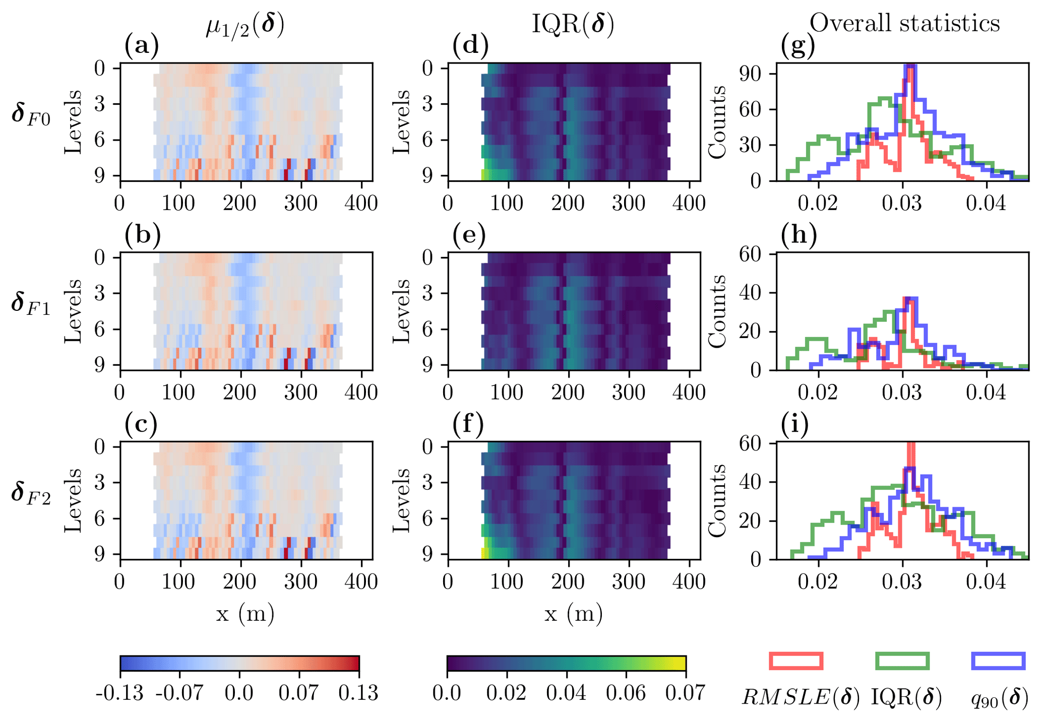
Figure 3 Summary statistics of the residuals for the Bykovsky data set corresponding to all models δ_F0 and for the two clustered families δ_F1 and δ_F2. (a–c) Median and (d–f) interquartile range calculated in a pixel-wise fashion. (g–i) Histograms illustrating the overall distribution of different statistical measures including RMSLE(δ), IQR(δ), and q₉₀(δ).

5.1.2 One-dimensional inversion of synthetic data

To complement our understanding of the formulated inverse problem, we perform 1D inversions of a synthetic data set created considering a 1D subsurface model (see “Input model” in Table 2) as described in Sect. 4.4. The 1D subsurface model parameters were chosen by analyzing our 2D model solutions (e.g., Fig. 2b–c at x≃150 m). We calculate the forward response of 10 quadripoles considering the same electrode configurations as used for recording the Bykovsky field data (Table 1). We invert the simulated apparent resistivity data using two scenarios for constraining z_w and ρ_w, while the constraints for all other parameters remain unchanged (see Table 2). The resulting inverted models are shown in Fig. 4a and c. For all models, we have achieved RMSLE <0.028, which is equivalent to the noise level applied to the calculated synthetic data and comparable to the RMSLE achieved for the 2D inversion results of the Bykovsky field data. Comparing the results shown in Fig. 4a and c illustrates that constraining the water layer significantly decreases the non-uniqueness of the inverse problem. We also notice that the median model represents a good approximation to the input model except for ρ_p, which is overestimated as illustrated by the larger ρ_p of the quantile 25 % model compared to the input ρ_p. Additionally, from all models visualized in Fig. 4a and c, we calculate the corresponding posterior correlation matrices (Fig. 4b and d). For both cases, we see that [ρ_uf, z_pt] is the model parameter pair with the highest positive correlation, while the rest of the model parameter pairs are characterized by negative correlations with different amplitudes (except for pairs with ρ_p which show correlations approaching zero).

Table 2 Parameters of the 1D synthetic model of Bykovsky and for two scenarios indicating the lower and upper bound parameter constraints.

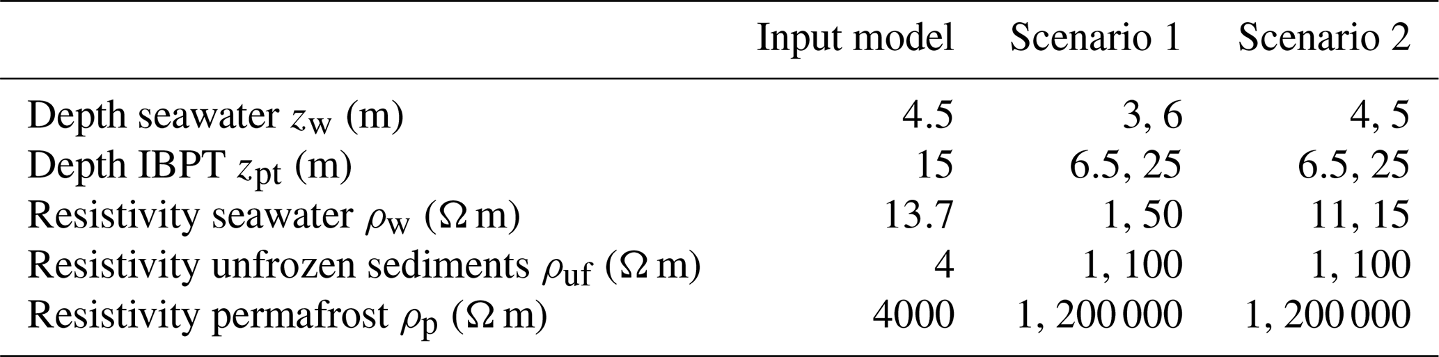
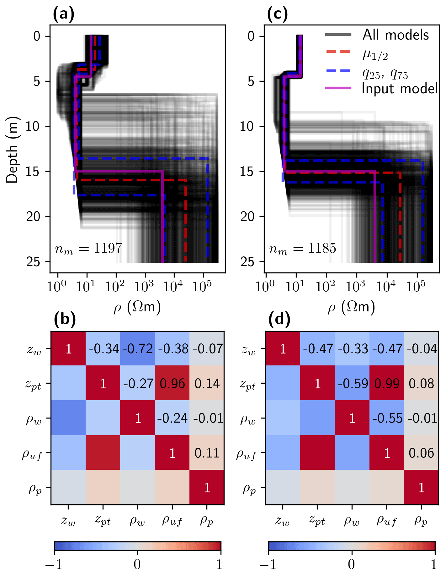
Figure 4 One-dimensional inversion results of synthetic data for 1D subsurface scenarios developed for the Bykovsky field site. (a) Ensemble with n_m model solutions and (b) the corresponding symmetric correlation matrix for scenario 1 (water layer parameters with large freedom during inversion) and (c–d) the same for scenario 2 (with constrained z_w and ρ_w). Black lines in panels (a) and (c) are plotted with transparency, and, therefore, the darker areas indicate higher densities model. The numbers in panels (b) and (d) are the corresponding correlation values.

5.1.3 Sensitivity analysis

To understand the sensitivity distribution for our three-layer model (representing seawater and unfrozen sediments overlying frozen sediments), we calculate the cumulative sensitivity and the sensitivity for the shortest and widest quadripoles considering two model scenarios (Fig. 5). In the first scenario, we consider the same input model as for the 1D inversion exercise (Table 2). In the second scenario, we set z_pt=25 m while all other parameters remain unchanged. From the cumulative sensitivity plots (Fig. 5a and d), we learn that areas of sensitivities extend throughout the layer of unfrozen sediments for both scenarios. This suggests that we could interpret our inverted models even underneath the outer electrode positions; i.e., if the boat together with the electrode streamer is moving toward the right (i.e., increased x coordinates) to collect additional sounding curves, our interpretation of the inverted model should start at $x\sim -\mathrm{60}$ m. Note that a more conservative model interpretation might start at $x\sim -\mathrm{25}$ m, where we start having more significant cumulative sensitivities. When analyzing Fig. 5b and e, we see that the shortest quadripole is sensitive to both the water layer and the unfrozen sediments. For a wider electrode spacing and an IBPT located at a depth of 15 m (Fig. 5c), the sensitivities are focused around the inner electrodes but also with some minor contributions from the outer electrodes (note the reddish colors in the unfrozen sediments at $x<-\mathrm{60}$ m and at x>60 m), which may be critical when significant 2D or 3D resistivity variations are present. For a deeper IBPT (Fig. 5f), we notice that we are still sensitive at depths of ∼25 m; however, the lateral extensions of the sensitivity patterns within the unfrozen sediments appear to be reduced.

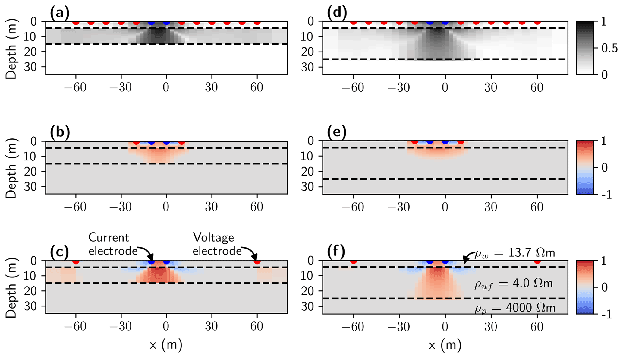
Figure 5 Two-dimensional normalized sensitivities for two different model scenarios developed for the Bykovsky field site. Position of the IBPT at a depth of (a–c) 15 m and (d–f) 25 m. From top to bottom, we show the cumulative sensitivity and the sensitivity for the shortest and widest quadripole, respectively.

As noticed in our 2D sensitivity analysis, the high resistivity contrast between the unfrozen and frozen sediments seems to limit the penetration depth down to the IBPT. To complement and better understand our results of 2D sensitivity analysis, we investigate the global sensitivities (Sect. 4.5) of different 1D model parameterizations. Specifically, we use models where z_w=4.5 m, ρ_w=13.7 Ω m, and ρ_uf=4 Ω m are fixed, while ρ_p varies between 10 and 10 000 Ω m (eight values in total) and the IBPT is located at three different depths; i.e., z_pt=25, z_pt=15, and z_pt=5 m (Fig. 6a–c). Note that defining eight different values for ρ_p and three for z_pt results in 24 different 1D models. For the calculation of the total sensitivity for each of our five parameters in these 24 models, we set the parameters ranges to $z_{\mathrm{w}}=[\mathrm{4},\mathrm{6}]$ m, $z_{\mathrm{pt}}=[\mathrm{6.5},\mathrm{30}]$ m, ${\mathit{\rho }}_{\mathrm{w}}=[\mathrm{0.2},\mathrm{20}]\mathrm{\Omega }$ m, ${\mathit{\rho }}_{\mathrm{uf}}=[\mathrm{1},\mathrm{20}]\mathrm{\Omega }$ m, and ${\mathit{\rho }}_{\mathrm{p}}=[\mathrm{5},\mathrm{20}\mathrm{000}]\mathrm{\Omega }$ m. For these specific models and parameter ranges, our results (Fig. 6) suggest ρ_w is the most influential parameter followed by ρ_uf, which shows approximately half of the influence compared to ρ_w. The influence of z_pt is slightly larger than z_w, although z_pt is set up with a wider range than z_w. Furthermore, although we allow ρ_p to vary over 3 orders of magnitude, the result of this sensitivity analysis demonstrates that ρ_p is the parameter with the lowest influence, but it is not null as indicated by the results of our 2D sensitivity analyses (Fig. 5a and d). Such low sensitivity values help to explain the large variation of ρ_p in our 1D and 2D ensembles. Interestingly, we also notice in Fig. 6a–c that in general when increasing ρ_p (for ρ_p<100 Ω m) the total sensitivity index of the other parameters tends to decrease.

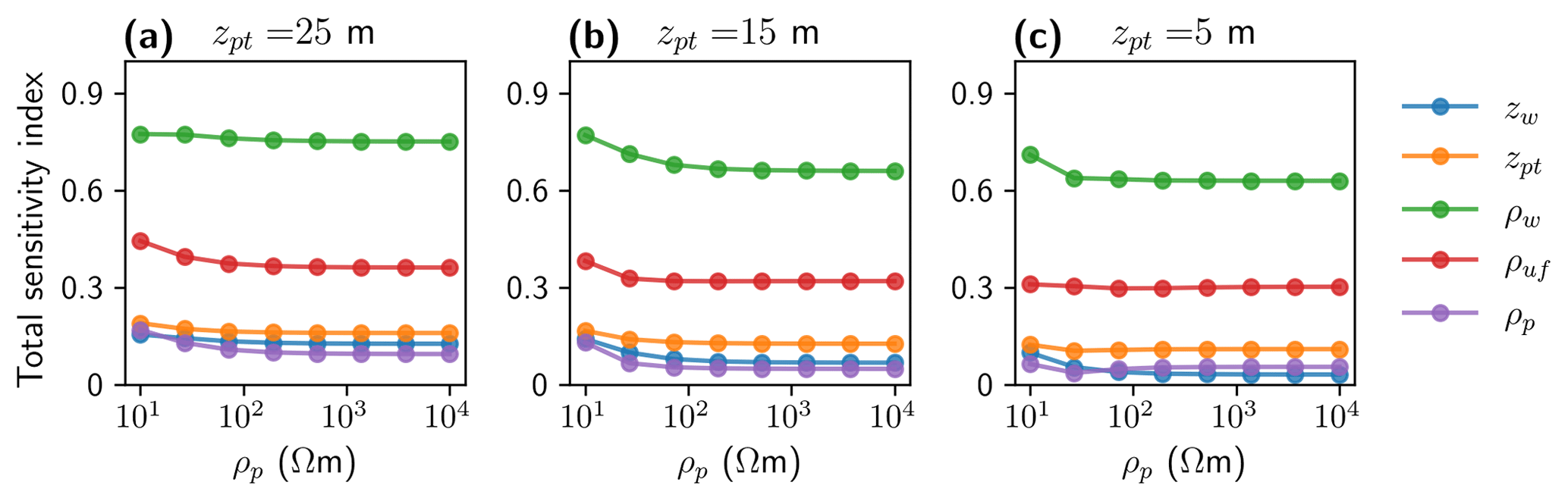
Figure 6 Global sensitivity results for the Bykovsky field site considering different 1D model scenarios with an IBPT at a depth of (a) 25 m, (b) 15 m, and (c) 5 m.

5.2 Drew Point

The geological and environmental settings of the Drew Point area are described in Sect. 2.2, and a summary of the acquisition parameters and measured seawater properties is provided in Table 1. We invert the 1830 apparent resistivity measurements recorded along an 854 m long profile (Fig. 1f) considering a layer-based model parameterization as described in Sect. 4.1 and a PSO-based inversion strategy as outlined in Sect. 4.2. In the PSO, because we notice that the inversion of the Drew Point data set converges much faster than in our Bykovsky example, we decide to lower the number of particles to 30 and the number of iterations to 400, thus allowing us to save some computational cost. Considering these settings, to obtain a single inverted model, we have to evaluate the forward response 12 000 times, which takes on average 57 h on a single core of a modern desktop computer. We repeat these inversion runs considering different initial seeds of the random number generator (using different processors in parallel) until we obtain an ensemble M_F0 consisting of 416 models.

5.2.1 Ensemble analysis

After the inversion, we interpolate all models to a refined structured mesh before performing any posterior statistical analyses (Sect. 4.3). In Fig. 7a and b, we present the ${\mathit{\mu }}_{\mathrm{1}/\mathrm{2}}\left({\mathit{M}}_{\mathrm{F}\mathrm{0}}\right)$ and IQR(M_F0) models calculated from the Drew Point model ensemble. The irregular variations in the IQR(M_F0) model and the bimodal distribution of ρ_p (some models with ρ_p<500 Ω m and others with ρ_p>100 000 Ω m) already indicate different groups of models with distinct resistivity characteristics and IBPT positions.

In the next step, we performed cluster analysis (Sect. 4.3) and found that our ensemble M_F0 can be divided into three model families (M_F1, M_F2, and M_F3). In Fig. 7b–d and f–h, we present the ${\mathit{\mu }}_{\mathrm{1}/\mathrm{2}}\left({\mathit{M}}_{\mathrm{Fi}}\right)$ and IQR(M_Fi) models (where $i=\mathrm{1},\mathrm{2},\mathrm{3}$). Comparing these models illustrates that M_F1 and M_F2 present a similar IBPT shape dipping toward the open sea. However, for M_F3 the IBPT position is dipping toward the coast, which is not in agreement with our background knowledge of this field site. When comparing the M_F1 and M_F2 models in more detail, we note that the IBPT position in M_F1 is shallower than in M_F2. Comparable to the Bykovsky example, models favoring high ρ_p values tend to show increased depths of the IBPT, resulting in thicker unfrozen sediments also near the coast. According to the depth of the IBPT and its gradients in the profile direction for M_F1 and M_F2, we laterally subdivide the model into four main parts. The first part is found at x<100 m, and it is characterized by an intermediate convex slope. The second part is found at $\mathrm{100}<x<\mathrm{500}$ m, and the IBPT shows a gentle convex slope, whereas in the third part (at $\mathrm{500}<x<\mathrm{700}$ m) the IBPT is almost flat. Finally, the fourth part is found at x>750 m, where the IBPT may be located at depths ≥20 m.

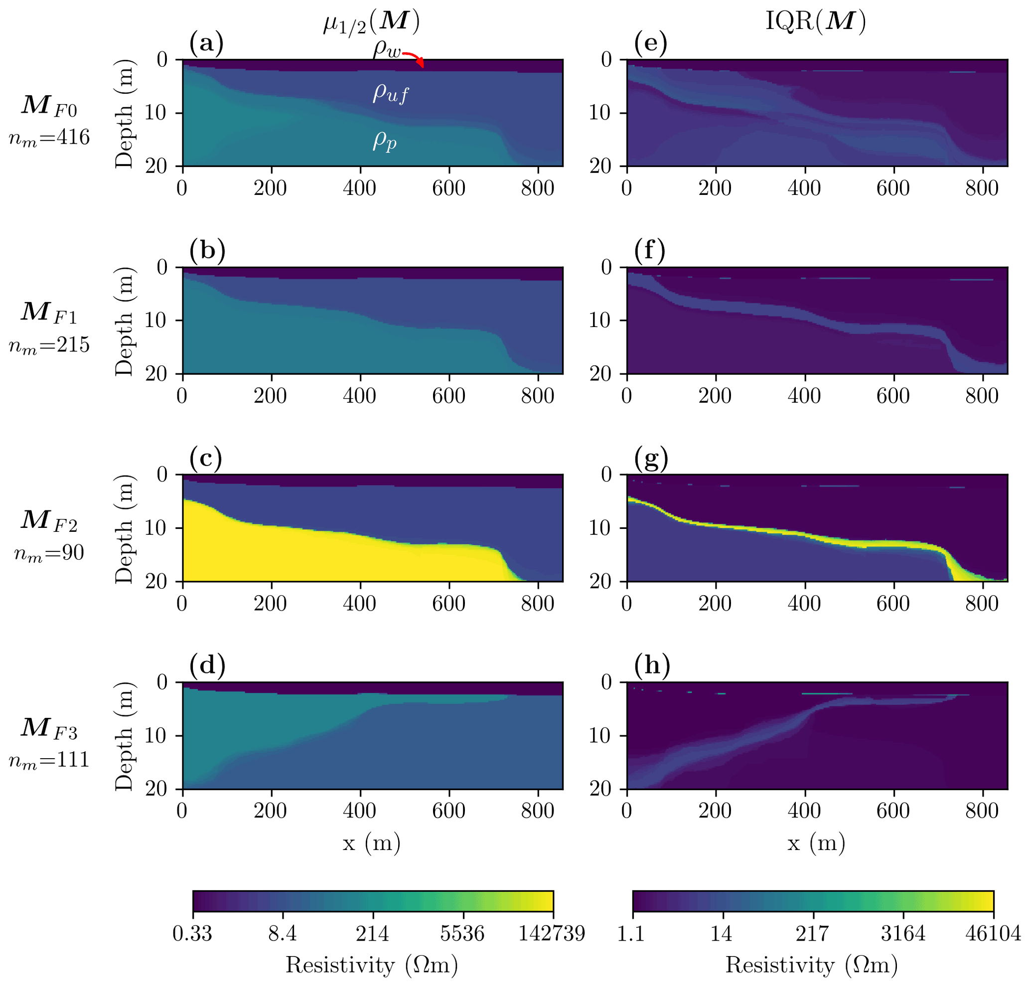
Figure 7 Inversion results for the Drew Point data set illustrated as summary statistics for all obtained models M_F0 and for three model families M_F1, M_F2, and M_F3 as found by cluster analysis. (a–d) Median and (e–h) interquartile range models. For each M_Fi, n_m represents the number of models in the corresponding ensemble.

We assess the fit performance for the residuals associated with the ensemble containing all models δ_F0, as well as for the three clustered model families δ_F1, δ_F2, and δ_F3 (Fig. 8). We calculate ${\mathit{\mu }}_{\mathrm{1}/\mathrm{2}}\left({\mathit{\delta }}_{\mathrm{Fi}}\right)$ and IQR(δ_Fi) (where $i=\mathrm{0},\mathrm{1},\mathrm{2},\mathrm{3}$) in a pixel-wise fashion and present them as pseudosections in Fig. 8a–h. When comparing these pseudosections to each other, we notice that ${\mathit{\mu }}_{\mathrm{1}/\mathrm{2}}\left({\mathit{\delta }}_{\mathrm{Fi}}\right)$ indicate similar fits of the data in terms of amplitudes and pseudosection patterns (although with slightly higher values for δ_F3). When comparing the IQR(δ_Fi) plots, we note that IQR(δ_F0) is characterized by several patches which are less prominent in the clustered residuals Fig. 8f–h. This indicates that our clustering results are properly grouping models with similar residuals. Furthermore, we associate the vertical feature at x=400 m in Fig. 8e–h to the variation in our models to locate the left edge of a bulge structure of the seabed (see Fig. 1e). This illustrates the applicability of exploring such residual statistics to identify possible drawbacks in our inversion results and, thus, allow us to re-evaluate our parameterization strategy. For example, we might consider to improve the inversion results by adding a node to our sums of arctangent functions around x=400 m. The overall statistics RMSLE(δ_Fi), IQR(δ_Fi), and q₉₀(δ_Fi) (where $i=\mathrm{0},\mathrm{1},\mathrm{2},\mathrm{3}$) are presented as histograms in Fig. 8i–l. The histograms in Fig. 8i are characterized by bimodal distributions. Such bimodal distributions are less pronounced for the clustered families (Fig. 8j–l); however, small tails to the right are also evident for δ_F1 and δ_F2. One may tend to reject the models falling in these tails, especially, when using the mean to estimate the central trend. However, because we consider robust statistical measures (e.g., median and IQR), we do not expect a significant impact from these models on our results and conclusions.

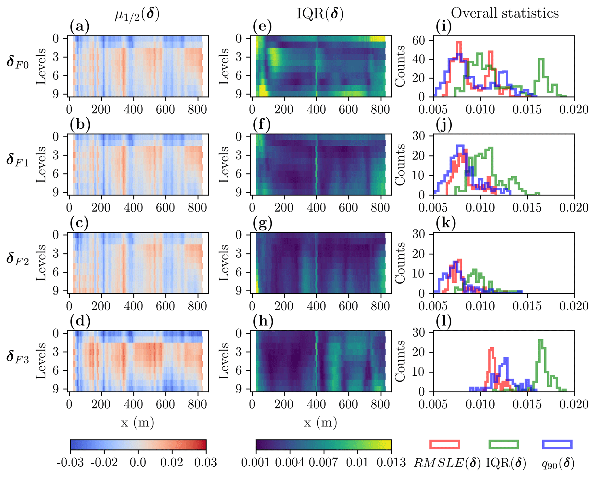
Figure 8 Summary statistics of the residuals for the Drew Point data set corresponding to all models δ_F0 and for the three clustered families δ_F1, δ_F2, and δ_F3. (a–d) Median and (e–h) interquartile range calculated in a pixel-wise fashion. (i–l) Histograms illustrating the overall distributions of different statistical measures including RMSLE(δ), IQR(δ), and q₉₀(δ).

Table 3 Parameters of the 1D synthetic model of Drew Point and for two scenarios indicating the lower and upper bound parameter constraints.

5.2.2 One-dimensional inversion of synthetic data

Following Sects. 4.4 and 5.1.2, we perform 1D inversions of a synthetic data set created considering a 1D subsurface model (see “Input model” in Table 3). The 1D model parameters were chosen by analyzing our 2D model solutions (e.g., Fig. 7b–c at x≈600 m). Note ρ_p is the same as in the 1D synthetic example from Sect. 5.1.2, which allows us to better compare the results of our 1D synthetic exercises. We calculate the forward response of 10 quadripoles considering the same electrode configurations as used for recording the Drew Point field data (Table 1). We invert the simulated apparent resistivity data considering two scenarios for constraining z_w, ρ_w, and ρ_uf, while the constraints for z_pt and ρ_p remain unchanged (see Table 3). The resulting inverted models are shown in Fig. 9a and c. For all models, we have achieved RMSLE <0.007, which is equivalent to the noise level applied to the calculated synthetic data and comparable to the RMSLE achieved for the 2D inversion results of the Drew Point field data. Comparing the results shown in Fig. 9a and c illustrates that the applied constraints improve the median model. However, we also observe an increase in the variability of the models around z_pt in Fig. 9c. Additionally, from all the models visualized in Fig. 9a and c, we calculate the corresponding posterior correlation matrix (Fig. 9b and d). For both cases, we see that the largest negative correlations are found for the model parameter pairs [ρ_uf, ρ_w] and [ρ_w, z_pt], while the most significant positive correlation is found for [ρ_uf, z_pt]. Note that the absolute correlations of these model parameter pairs are larger in Fig. 9d compared to Fig. 9c. Finally, we want to point out that the signs for the most significant parameter correlations are the same as the ones found for Bykovsky in Fig. 4d.

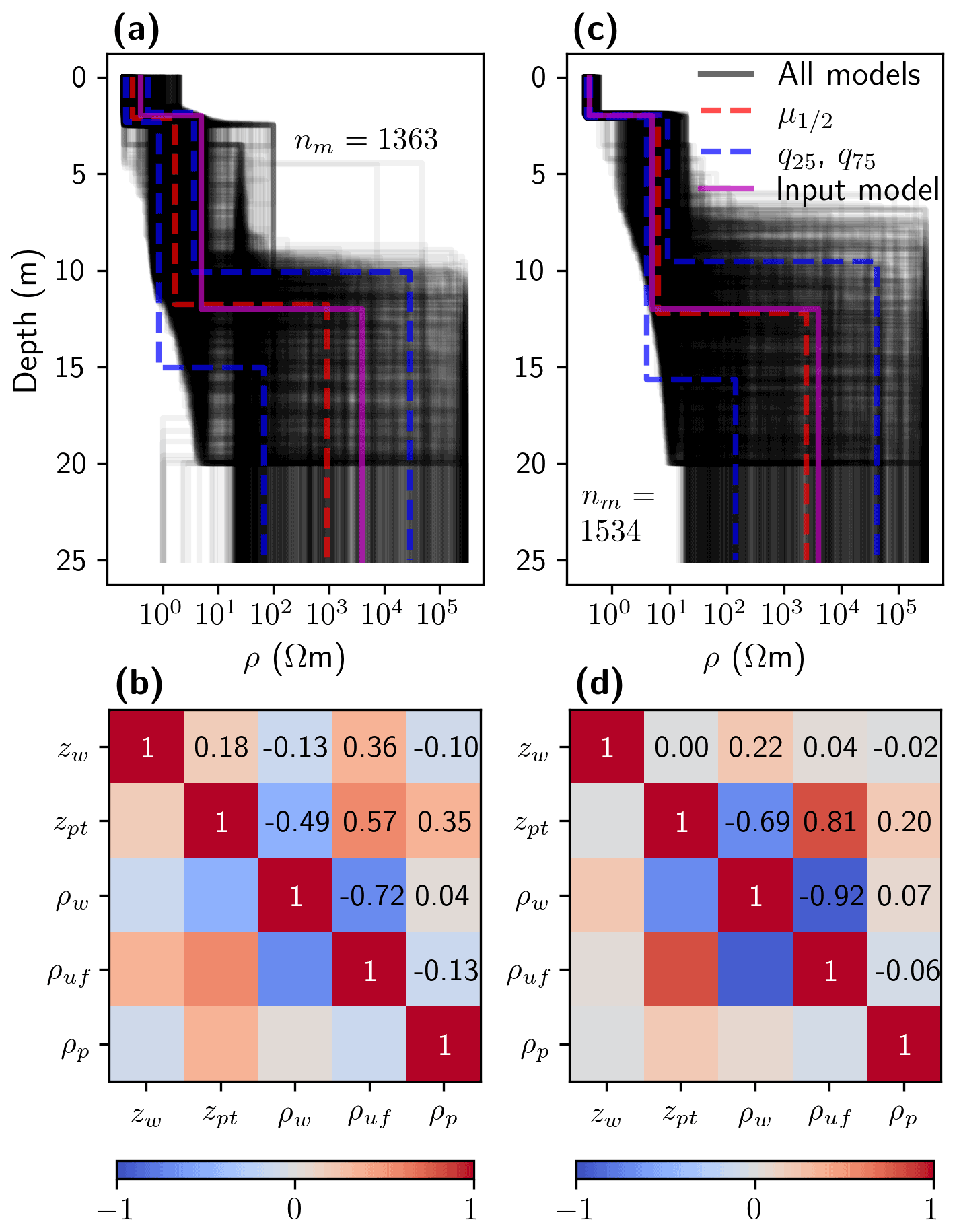
Figure 9 One-dimensional inversion results of synthetic data for 1D subsurface scenarios developed for the Drew Point field site. (a) Ensemble with n_m model solutions and (b) the corresponding symmetric correlation matrix for scenario 1 (water layer parameters with large freedom during inversion) and (c–d) the same for scenario 2 (with constrained z_w, ρ_w, and ρ_uf). Black lines in panels (a) and (c) are plotted with transparency, and, therefore, the darker areas indicate higher densities model. The numbers in panels (b) and (d) are the corresponding correlation values.

5.2.3 Sensitivity analysis

For the sensitivity analysis, we consider the two model scenarios indicated in Fig. 10. In the first scenario, we consider the same input model as for the 1D inversion exercise (Table 3). In the second scenario, we set z_pt=16 m while all other parameters remain unchanged. From analyzing the cumulative sensitivity plots (Fig. 10a and d), we infer that an interpretation of our inversion results should focus on the area around the inner electrodes; i.e., if the boat is moving toward the right to collect additional sounding curves, our interpretation of the inverted model should start at $x\sim -\mathrm{10}$ m. When analyzing Fig. 10b and e, we see that we are most sensitive to the water layer. Interestingly, when comparing Fig. 10c and f in detail, we realize that the sensitivity distribution in Fig. 10c reaches the IBPT interface while the sensitivity distribution in Fig. 10f is almost null for depths >12 m.

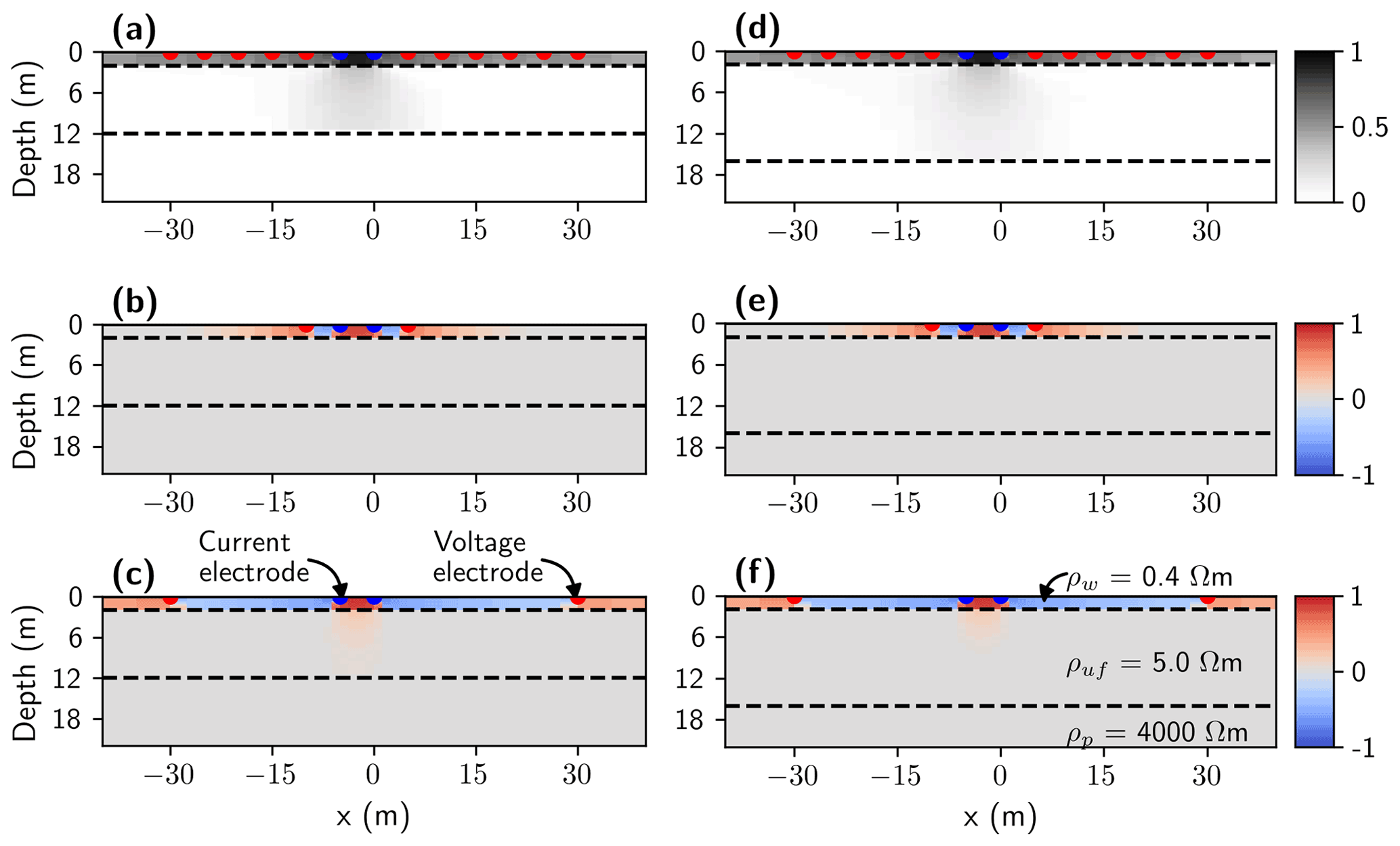
Figure 10 Two-dimensional normalized sensitivities for two different model scenarios developed for the Drew Point field site. Position of the IBPT at a depth of (a–c) 12 m and (d–f) 16 m. From top to bottom, we show the cumulative sensitivity and the sensitivity for the shortest and widest quadripole, respectively.

We perform the global sensitivity analyses (Sect. 4.5) considering 1D models described by five model parameters as used for the above-presented 1D inversions. We consider models where z_w=2 m, ρ_w=0.4 Ω m, and ρ_uf=5 Ω m are fixed, while ρ_p varies between 10 and 10 000 Ω m (eight values in total), and the IBPT is located at three different depths; i.e., z_pt=16, z_pt=10, and z_pt=4 m (Fig. 11a–c). For the calculation of the total sensitivity for each of our five parameters in the resulting 24 models, we set the parameter ranges to $z_{\mathrm{w}}=[\mathrm{0.5},\mathrm{3}]$ m, $z_{\mathrm{pt}}=[\mathrm{3.5},\mathrm{20}]$ m, ${\mathit{\rho }}_{\mathrm{w}}=[\mathrm{0.2},\mathrm{20}]$ Ω m, ${\mathit{\rho }}_{\mathrm{uf}}=[\mathrm{1},\mathrm{20}]$ Ω m, and ${\mathit{\rho }}_{\mathrm{p}}=[\mathrm{5},\mathrm{20}\mathrm{000}]$ Ω m. For these specific models and parameters ranges, our results (Fig. 11) suggest that ρ_w and ρ_uf are the most influential parameters, and the other three parameters (z_pt, z_w and ρ_p) are characterized in all cases by rather low total sensitivities. Furthermore, we also notice in Fig. 11a–c that ρ_w is the parameter showing the most significant changes when varying ρ_p and z_pt.

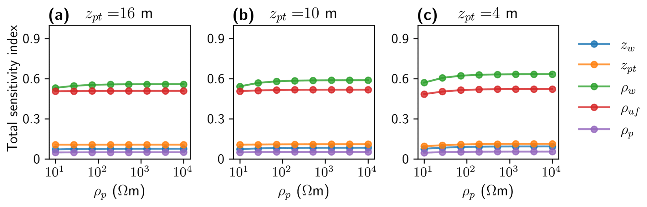
Figure 11 Global sensitivity results for the Drew Point field site considering different 1D model scenarios with an IBPT at a depth of (a) 16, (b) 10, and (c) 4 m.

6 Discussion

Knowledge of how fast permafrost thaws would improve predictive models of greenhouse gas release and coastal erosion, as well as coastal infrastructure design. The ERT method has been successfully used to image the unfrozen sediments overlying the permafrost layer in subsea permafrost environments, especially using smooth inversion approaches (e.g., Overduin et al., 2012; Pedrazas et al., 2020). In typical subsea permafrost environments, there might be a gradual transition zone consisting of a mixture of water and ice between fully unfrozen and frozen ice-bonded sediments. However, during ERT inversion, the nature of this transition can be either enlarged when using smooth inversion approaches or reduced to a single interface when using layer-based strategies. Whether we have a smooth or sharp transition between unfrozen and frozen sediments, there must be a threshold in the ice content that creates sufficient contrast in resistivity also influencing the penetration of the injected current and, thus, our apparent resistivity measurements (e.g., Kang and Lee, 2015). Because we wanted to target the interface defined by such a resistivity contrast (interpreted here as the IBPT), we considered a layer-based model parameterization to invert our ERT data. Additionally, we obtained estimates of uncertainties using an ensemble approach. For the sake of completeness, we provide the smooth inversion models for both of our field studies in Appendix A.

6.1 Insights from our parameterization and inversion strategies

We used a 2D layer-based model parameterization to globally invert marine ERT data and obtain different ensembles (e.g., after cluster analysis) of model solutions. We demonstrated with the two case studies that such ensembles allow us to reliably image the IBPT position with its associated uncertainties. The main advantage of using a layer-based model parameterization strategy is that we do not assume an arbitrary resistivity threshold or gradient to interpret the IBPT position, as we would need to do for our smooth inversion results (see Fig. A1a–b). This may be advantageous to compare ERT profiles collected at the same position in different years to track changes along the IBPT or in environments where the freezing point of the sediment porewater changes spatially. For example, offshore surveys that encounter submerged hypersaline lagoon deposits may show relatively low resistivity values for partially frozen sediments compared to colder ice-bonded permafrost with fresh porewater (Angelopoulos et al., 2021). Indeed, this interface may be related to a threshold in ice content. However, associating the IBPT with a certain ice content requires calibration by using borehole data or by additional geophysical information; e.g., by using the joint inversion approach of ERT and seismic refraction data of Wagner et al. (2019). Such thresholds may vary from site to site depending on properties of the sediments including temperature, grain size distribution, and the salinity of the porewater. Furthermore, we consider it convenient to use the sum of arctangent functions to parameterize the IBPT because there may be cases where the IBPT position varies steeply (as the ones we identified at the end of the median models in Figs. 2a–c and 7a–c) associated, for example, with submerged thermokarst structures or changes in the ratio of coastal erosion vs. degradation rate.

To find reliable and stable 2D model solutions, we performed experiments in which we ran the PSO several times to find the appropriate parameter settings for our layer-based ERT inversion. In a first stage, when performing our 2D inversions without considering any constraints, we found model solutions that were unrealistic according to our prior knowledge of our field sites. Therefore, we constrained our inversions considering our bathymetric and CTD measurements (see Sect. 4.2). Although the 2D inverted models without considering constraints are not shown in this study, we demonstrated with our 1D inversions how such constraints significantly improved the inversion results while reducing the number of possible solutions. Another exercise in the experimental phase consisted in using more than three layers in our parameterization strategy. However, we did not observe any significant improvement in the final median models when increasing the number of layers and, thus, restricted our inversion and analyses to three-layer scenarios.

One disadvantage of using a layer-based model parameterization relying on homogeneous layers is that it is not possible to resolve small-scale resistivity variations (e.g., horizontal heterogeneities at a spatial scale of meters). However, our workflow allowed us to inspect and evaluate model performance including the appropriateness of the model parameterization. For example, in the Bykovsky and Drew Point case studies, we observed in the residual pseudosections some regular lateral variations (see Figs. 3 and 8). This indicates that we were not completely explaining the data, because of either lateral subsurface resistivity variations or 3D effects. To tackle this problem, it could be beneficial to measure 3D bathymetric data around each ERT profile and collect additional parallel and perpendicular ERT profiles to better understand 3D resistivity variations at our field sites. Furthermore, direct measurement of the resistivity of water and unfrozen sediments (e.g., using additional water samples and drilling cores) might help to inform the model parameterization (e.g., account for lateral variations) and inversion strategies. We should notice that adding complexity to our model parameterization comes with the trade-off of increased computational cost to solve the inverse problems. An alternative to obtaining more complex resistivity models is to use our layer-based global inversion results as reference models to perform smoothness-constrained inversions (e.g., Günther et al., 2006).

The error level of ERT data is usually unknown – especially for marine data, where repeated or reciprocal measurements are not practical because the data are acquired while the boat is moving. This represents a challenge during the inversion when specifying an appropriate fit level. One alternative to get insights into the noise level is to perform repeated measurements in a static fashion (avoiding bending of the cable by wind or swells) for a certain section of the profile. For example, this can be achieved at the coast on a calm day where one end of the cable is secured to the beach and the other end is fastened to an anchored boat. However, such repeat measurements were not available for our field sites. Therefore, we set our stopping criterion by considering a fixed number of iterations rather than using a minimum threshold in our objective function. With this approach, we obtained model solutions characterized by different fit levels. For example, for the Bykovsky data, we found RMSLE values between 0.025 and 0.038 (Fig. 3g–i), while for our Drew Point data, we found RMSLE values between 0.007 and 0.016 (Fig. 8i–l). Although the RMSLE values for Drew Point are significantly lower than for Bykovsky, we found a family of models in the Drew Point study, which was considered as geologically unrealistic (Fig. 7d). This highlights the importance of estimating different ensembles of solutions with different fit levels and having an accurate estimate of data noise. Because the misfits for the model in Fig. 7d were higher, this family of models could potentially be discarded if they were found to exceed expected error levels without considering any prior knowledge of the environmental setting.

6.2 Parameter learning from 1D inversion

Our 2D inversion results showed large variations in the modeled resistivities of the permafrost, and we also noticed that, typically, the variabilities of IBPT position increase with depth. These observations indicate decreasing resolution capabilities of our ERT data with depth and limited penetration of the injected current in the frozen permafrost layers. To better understand these results in a more quantitative fashion, we reduced the number of parameters to five and performed selected 1D inversion experiments using synthetic data inspired by our 2D inversion results. Because such 1D inversions are significantly faster than 2D inversions, they represent an efficient way to explore the influence of constraining different parameters. For example, we noticed from our 1D inversion results that constraining the water layer significantly decreased the non-uniqueness of the inverse problem. This is essential for a reliable estimation of the IBPT position and for establishing petrophysical relations, for example, to estimate porewater salinity and ice content. Additionally, we noticed that the 1D inversion results for the Bykovsky data (Fig. 4c) provided similar uncertainties around the IBPT as the 2D inversion results at x=150 m (Fig. 2d–f). However, the 1D inversion results for the Drew Point data (Fig. 9c) showed uncertainties around the IBPT 3 times larger compared to the 2D inversion results at x≈600 m (Fig. 7f and g). This indicates that there is no general best way of using the results of such complementary synthetic 1D studies; the success and feasibility rather depends on the characteristics of the field site and analyzed data set. On the other hand, we can use our 1D inversion results to assess the posterior correlation matrix that, as we showed in our examples, can be helpful to identify interactions between the model parameters. Furthermore, comparing the changes across different posterior correlation matrices (e.g., associated with different model constraints) can help us detect changes in the parameters interactions and, thus, quantify the impact of our model constraints. Such straightforward but informative analysis provides a deeper understanding of the inversion process and the suitability of the entire inversion strategy.

Our 1D inversion results indicated some problems if we want to infer relative permafrost characteristics from ERT measurements. The 1D input models for our 1D synthetic examples (see Tables 2 and 3) assumed identical resistivities of the ice-bearing permafrost layer (ρ_p=4000 Ω m) and similar resistivities for the unfrozen sediments as found by our 2D inversion results. In contrast, the resistivity and depth of the seawater layer between both models were set according to field measurements at our field sites. Although the resistivities of the unfrozen and frozen layers were similar in both models, we noticed that for model scenarios derived from the Bykovsky site, the inverted ρ_p values were generally overestimated where already the q₂₅ model indicates ρ_p values larger than the input ρ_p (Fig. 4c). On the contrary, for settings inspired by the Drew Point field site, the input ρ_p fell within the range defined by q₂₅ and q₇₅ models but showed more significant variabilities than our 1D Bykovsky experiment (Fig. 9c). These results demonstrated the influence of the depth and resistivity of the seawater layer in the inverted models which may be critical for subsequent interpretations. For example, assuming the same temperature and porewater salinity, the resistivity of the sediments increases with ice content (e.g., Pearson et al., 1986; Fortier et al., 1994; Kang and Lee, 2015). Thus, our results may lead us to conclude that the ice-bearing permafrost layer holds higher ice content at Bykovsky compared to Drew Point. Over- or underestimating the ice-bearing permafrost resistivity may lead to potentially erroneous interpretations, for example, related to the sediment's ice content, temperature, and composition. We would need complementary field information or further analyses like sensitivity assessments to avoid misleading interpretations.

6.3 System understanding with sensitivity analysis

We obtained an additional model understanding (e.g., in view of delineating confident and reliable model areas) by performing sensitivity analyses. From our examples, we learned that if the resistivity of the seawater were higher than the resistivity of the unfrozen sediments (as in the Bykovsky case study, Fig. 5), this would result in increased sensitivities inside the unfrozen sediments and, thus, to changes along the IBPT position. This type of situation may be prevalent in subsea permafrost areas affected by freshwater river discharge in summer. On the other hand, if the seawater were less resistive than the unfrozen sediments (e.g., as in the Drew Point case study, Fig. 10), we would be more sensitive to the water layer and, therefore, to bathymetric changes. This emphasizes the importance of accurate water depth measurements. We highlight the fact that although the local 2D sensitivities for the Drew Point data were rather small for the unfrozen sediments, the IQR of the models (Fig. 7f–g) showed equivalent variability around the depth of IBPT (1.5 to 2 m for depths ∼12 m) in comparison to the Bykovsky example (Fig. 2d–f), where the sensitivities showed a more pronounced influence within the unfrozen sediments.

This study used global sensitivity analysis considering only five parameters as needed for our 1D inversion examples. The Sobol approach proved to be a powerful method to distinguish the most influential parameters. After evaluating how the permafrost resistivity and the IBPT position may influence the rest of the parameters in our 1D three-layer examples, we noted some relevant differences. For example, in the Bykovsky example (Fig. 6), we noticed that for larger values of ρ_p and shallower z_pt the total influence of the rest of the parameters decreased. On the other hand, for the Drew Point example (Fig. 9), increasing ρ_p increased the total sensitivity of the rest of the parameters, while varying z_pt at shallower depths mainly increased the influence of ρ_w. We also want to highlight that ρ_w, ρ_uf, and z_pt were the parameters with the most significant total sensitivity in both examples and were also the parameters that formed model parameter pairs showing the largest correlation (see Figs. 4d and 9d). Encouragingly, ρ_w and ρ_uf can be informed from CTD casts and shallow sediment sampling, respectively. We must be aware that such a global sensitivity analysis is highly dependent on the predefined constraining parameter range and should be applied to address specific questions to allow, for example, parameter reduction or to guide our sampling strategies and experimental design.

6.4 Subsea permafrost features (Bykovsky vs. Drew Point)

The inverted ERT profiles yielded new insights into how subsea permafrost thaws because the Bykovsky Peninsula and Drew Point are characterized by distinct seawater properties and geological histories. The Bykovsky 2D inversion results at x=150 m, which corresponds to an inundation period of 357 years assuming an erosion rate of 0.42 m yr⁻¹ (e.g., Lantuit et al., 2011), showed a median depth to the IBPT of ∼15 m (Fig. 2). This resulted in an average degradation rate of ∼0.04 m yr⁻¹. On the other hand, the Drew Point 2D inversion results at x≈600 m showed a median depth to the IBPT of ∼12 m. Note that this location coincides with the 1955 coastline position (see Fig. 1d–e), which corresponds to 63 years of inundation, yielding an average degradation rate of ∼0.19 m yr⁻¹. At Bykovsky, 63 years of inundation (again assuming an erosion rate of 0.42 m yr⁻¹) correspond to an offshore distance of ∼26 m, which corresponds to a median IBPT depth in the 2D inversion results at most 6 m (Fig. 2). Although the mean annual IBPT degradation rate slows with inundation time as the temperature gradient driving diffusive heat fluxes weakens (Angelopoulos et al., 2019), it is evident that the permafrost at Drew Point may thaw faster, presumably because Drew Point sediments are primed with salts in the pore space prior to inundation (Black, 1964; Sellmann, 1989).

Since salt diffusion is typically slower than heat diffusion (Harrison and Osterkamp, 1978), the IBPT degradation rate at Bykovsky should theoretically be faster than at Drew Point, provided that the permafrost sediments are similar. However, it appears that dissolved salts in the pore space of the sediments at Drew Point play an important role in lowering the permafrost freezing point and resulting in higher IBPT degradation rates than at Bykovsky. In fact, the top of onshore cryotic and saline unfrozen sediment layers (cryopegs) were observed near the Drew Point shoreline during coring (Bull et al., 2020; Bristol et al., 2021). This can lead us to interpret a faster IBPT degradation rate at Drew Point compared to Bykovsky in two ways: (1) a layer of submerged Drew Point sediments was already unfrozen upon inundation (e.g., M_F2 in Fig. 7) and (2) the frozen layers at Drew Point contained less ice and had a lower freezing point. Jones et al. (2018) suggested that warming permafrost temperatures at Drew Point (3 to 4 ^∘C over the past several decades) have made saline permafrost more susceptible to erosion, potentially contributing to the enhanced coastal erosion rate (2.5 times that of the historical average) observed between 2007 and 2016. Warming by seawater submergence would presumably result in cryopeg spreading and IBPT degradation.

As shown in Fig. 1a and d, the coastal plains at our field sites consist of numerous thermokarst lakes and drained lake basins. When thermokarst lakes are breached by coastal erosion, the unfrozen sediments underneath the lake become integrated into the subsea permafrost environment, leading to bowl-shaped electrical resistivity structures. For example, Angelopoulos et al. (2021) showed steep IBPT gradients along ERT profiles parallel to the southern Bykovsky shoreline that traverse submerged thermokarst and undisturbed permafrost. These authors also suggested that drained lake basins, which have undergone thaw–refreeze cycles, are more susceptible to quicker thaw compared to undisturbed terrain. Comparing the first 400 m of our inverted median models for our field sites, we noticed that, in general, the IBPT at Drew Point is smoother than at Bykovsky. This might be the result of the higher erosion rates at Drew Point (>10 m yr⁻¹) than at Bykovsky (<1 m yr⁻¹) that expose coastal areas to inundation in a shorter time. Because of the longer inundation time at Bykovsky, we expect fluctuations in different environmental controls (e.g., water temperature, seawater salinity) that might result in step-like features as the one at x≈280 m. Furthermore, layered strata alternating between ice-rich and relatively ice-poor sediment may also contribute to step-like IBPT features. Similarly, in the Drew Point 2D inversion (Fig.  7a–c), there was a steep median IBPT decline observed at x≈750 m, where the IBPT deepened from ∼12 to ≥20 m. Although the resolution capabilities of our ERT data at these depths are limited, we suggest that thermokarst processes prior to seawater submergence may be responsible for the nature of this IBPT dip.

7 Conclusions

In this study, we illustrated how we could use ERT data to reliably estimate the IBPT position in shallow coastal areas of the Arctic. We found that using a layer-based model parameterization helps us target the IBPT position directly from the inversion of ERT data with the trade-off of omitting small-scale heterogeneities. To improve the inversion result, we noticed that constraining the water layer depth and resistivity reduces the non-uniqueness of the ERT inverse problem, improving the estimation of the resistivity of the unfrozen sediments (talik and/or cryopeg) and the IBPT position. However, even when constraining the water layer, we still found large variabilities in the resistivity of the frozen sediments. We suggest that constraining the resistivity of the unfrozen sediments (e.g., sediment sampling) during ERT inversion could improve resistivity estimates of the frozen layer and, thus, further permafrost's physical properties (e.g., ice content). Properly imaging the IBPT position may allow us to improve the estimation of the permafrost degradation rate, which might be used to better understand greenhouse gas emissions and coastal erosion processes. The workflow and methods presented in this study can guide future field campaigns and may be used as a reference for more detailed parameterizations and/or inversion strategies.

Appendix A: Smooth inversion

Although comparing different inversion strategies is beyond the scope of this study, for the sake of completeness, we show the smooth inversion results for our Bykovsky and Drew Point data sets in Fig. A1a–b. To invert these data sets, we use the inversion routine of the Python library pyGIMLi (Rücker et al., 2017). For both cases, we constrain the seawater layer by using the bathymetric profile data as collected by a Garmin echo sounder (see Sect. 3). The Bykovsky model (Fig. A1a) shows the highest resistivities to the left (near the coast), while resistivities drop in the offshore direction. For our Drew Point model (Fig. A1b), the highest resistivities are also present near the coast, but the resistivities decrease in the offshore direction more gradually than in the Bykovsky model. To derive the IBPT position from these models, we would need to assume or measure (e.g., through borehole data) the resistivity threshold that separates the talik from the ice-bearing permafrost layer (e.g., Overduin et al., 2016; Sherman et al., 2017; Angelopoulos et al., 2021). Because no ground-truth data are available and to avoid assuming a resistivity threshold, we decide to target such an interface using a layer-based model parameterization approach as explained in Sect. 4.1. Please refer to Angelopoulos et al. (2019), where a smooth inversion of the Bykovsky data set presented in this study is discussed in more detail, as well as Angelopoulos et al. (2021), where laterally constrained inversions of additional data sets offshore of Bykovsky are shown.

Figure A1 Smooth inversion models for (a) the Bykovsky and (b) Drew Point data sets. To enhance the resistivity contrast in our ERT models presented in panels (a) and (b), we limited the lower and upper resistivities considering quantiles 0.04 and 0.96, respectively.