the Creative Commons Attribution 4.0 License.
the Creative Commons Attribution 4.0 License.
 | 04 Feb 2022
Relating snowfall observations to Greenland ice sheet mass changes: an atmospheric circulation perspective
Michael R. Gallagher
Matthew D. Shupe
Hélène Chepfer
Tristan L'Ecuyer
Snowfall is the major source of mass for the Greenland ice sheet (GrIS) but the spatial and temporal variability of snowfall and the connections between snowfall and mass balance have so far been inadequately quantified. By characterizing local atmospheric circulation and utilizing CloudSat spaceborne radar observations of snowfall, we provide a detailed spatial analysis of snowfall variability and its relationship to Greenland mass balance, presenting first-of-their-kind maps of daily spatial variability in snowfall from observations across Greenland. For identified regional atmospheric circulation patterns, we show that the spatial distribution and net mass input of snowfall vary significantly with the position and strength of surface cyclones. Cyclones west of Greenland driving southerly flow contribute significantly more snowfall than any other circulation regime, with each daily occurrence of the most extreme southerly circulation pattern contributing an average of 1.66 Gt of snow to the Greenland ice sheet. While cyclones east of Greenland, patterns with the least snowfall, contribute as little as 0.58 Gt each day. Above 2 km on the ice sheet where snowfall is inconsistent, extreme southerly patterns are the most significant mass contributors, with up to 1.20 Gt of snowfall above this elevation. This analysis demonstrates that snowfall over the interior of Greenland varies by up to a factor of 5 depending on regional circulation conditions. Using independent observations of mass changes made by the Gravity Recovery and Climate Experiment (GRACE), we verify that the largest mass increases are tied to the southerly regime with cyclones west of Greenland. For occurrences of the strongest southerly pattern, GRACE indicates a net mass increase of 1.29 Gt in the ice sheet accumulation zone (above 2 km elevation) compared to the 1.20 Gt of snowfall observed by CloudSat. This overall agreement suggests that the analytical approach presented here can be used to directly quantify snowfall mass contributions and their most significant drivers spatially across the GrIS. While previous research has implicated this same southerly regime in ablation processes during summer, this paper shows that ablation mass loss in this circulation regime is nearly an order of magnitude larger than the mass gain from associated snowfall. For daily occurrences of the southerly circulation regime, a mass loss of approximately 11 Gt is observed across the ice sheet despite snowfall mass input exceeding 1 Gt. By analyzing the spatial variability of snowfall and mass changes, this research provides new insight into connections between regional atmospheric circulation and GrIS mass balance.
- Article
(8033 KB) - Full-text XML
- BibTeX
- EndNote


The Greenland ice sheet (GrIS) is currently the leading cause of global sea level rise, contributing an average increase of 0.47 mm each year in the years since 2000 (Shepherd et al., 2012; Van Den Broeke et al., 2016). Because of this contribution to sea level rise, GrIS mass balance plays an important role in the Earth-climate system. While mass loss can result from a range of complex processes, snowfall is the major source of GrIS mass gain and is the largest control on inter-annual variability of GrIS mass balance (van den Broeke et al., 2009). Yet, because measurements are difficult to obtain, snowfall over the GrIS is poorly constrained, and snowfall is difficult to model accurately, our understanding of snowfall's contribution to mass balance remains limited and uncertain (Noël et al., 2015; Vernon et al., 2013).
Previous studies have utilized models to show that mass input via snowfall over the GrIS is closely tied to atmospheric dynamics, with atmospheric circulation being the primary contributor to snowfall and accumulation variability (Noël et al., 2015; Danco et al., 2016). In terms of both snowfall mass input and ablation, research indicates that the GrIS is particularly sensitive to atmospheric variability on synoptic timescales (Schuenemann and Cassano, 2010; Doyle et al., 2015; Neff et al., 2014; Mattingly et al., 2018; Gallagher et al., 2020). Although these event-based studies have greatly improved our understanding of the relationship between the atmosphere and GrIS mass balance, few studies have focused on the impact of such events on snowfall. Important steps in this direction have been taken at specific Greenland in situ observation sites (Pedersen et al., 2018; Pettersen et al., 2018), but the connections between observed spatial variability in snowfall and atmospheric circulation have yet to be examined. This analysis intends to broaden our understanding in this area, by relating atmospheric circulation to its impact on snowfall and changes in mass balance.
Recently researchers have begun to analyze CloudSat-derived estimates of snowfall across the Arctic, with Bennartz et al. (2019) and Ryan et al. (2020) studying the spatial and temporal variability of snowfall over Greenland and research by Edel et al. (2020) contextualizing snowfall across the broader Arctic climate. Work from McIlhattan et al. (2020) takes this a step further by analyzing detailed cloud properties and their impact on snowfall but does not investigate relationships with atmospheric circulation in a detailed manner. Thus, while these studies have provided important insight into Arctic snowfall, the work presented here advances this line of research by directly connecting the daily variability of atmospheric circulation to snowfall and its impact on Greenland ice sheet mass balance. Specifically, we relate the spatial and temporal variability of snowfall across the GrIS to the daily variability of regional atmospheric circulation regimes. By utilizing novel data products from CloudSat spaceborne radar observations of snowfall (Wood and L'Ecuyer, 2021) and categorizing local circulation patterns using self-organizing maps (SOMs), we assess the impact of the atmosphere on snowfall spatial variability across the GrIS and quantify snowfall mass input to the GrIS. Finally, by incorporating observations from the Gravity Recovery and Climate Experiment (GRACE), the snowfall mass input is more broadly contextualized to reveal the relationship between snowfall, atmospheric circulation, and daily GrIS mass changes. The work presented here is a significant step beyond previous research looking at average seasonal mass balance changes in the context of the North Atlantic Oscillation, primarily because of the daily temporal resolution resulting from the unique methodology.
2.1 CloudSat snow product
We utilized snowfall observations from the CloudSat spaceborne Cloud Profiling Radar (CPR) (Im et al., 2005; Stephens et al., 2008, 2018), a single-frequency 94 GHz W-band radar. CloudSat orbits at an inclination of 98.2∘, and the CPR has a spatial resolution of 1.4×1.8 km. CloudSat data used in this analysis were obtained from the fifth release of the 2C-SNOW-PROFILE data product. This product uses a Bayesian estimation retrieval algorithm to estimate vertical properties of snowfall from reflectivity profiles measured by the CPR (Wood et al., 2013, 2014). CloudSat observations from 1 June 2006 to 16 April 2011 were used here. Because this analysis requires uniform intra-annual data to investigate seasonal variability in the Arctic, utilizing observations from the period after the April 2011 CloudSat battery anomaly was not possible as the satellite could no longer obtain winter observations during polar night.
Previous research has determined CloudSat to be well suited for observing the light snow common at high latitudes such as over the GrIS (Cao et al., 2014; Norin et al., 2015). Because this study is concerned with the impact of snowfall on GrIS mass balance, snowfall rates are used from the 2C-SNOW-PROFILE product. Snowfall rates near the surface are not available due to ground clutter interfering with the CPR; thus, these snowfall rates are derived from the fourth bin above the land surface. This is the first bin not contaminated by ground clutter typically located roughly 1 km above the Earth's surface. This gap is known as the snowfall “blind zone”, and it results in an approximately 10 % underestimation of snowfall amounts in polar regions (Maahn et al., 2014). Despite this blind zone, research has shown that CloudSat observations are closely correlated with mass accumulation at the GrIS surface, and they are currently the best available spatial measurements of snowfall (Bennartz et al., 2019; Ryan et al., 2020).
While CloudSat can potentially saturate during heavy snowfall, snowfall events of this magnitude are rare over the GrIS. The snowfall rates presented here are from above the ground-clutter zone and are assumed to statistically represent the snowfall at the GrIS surface. CloudSat snowfall observations are provided in units of millimeters per hour (mm/h), but when used here the resulting snowfall averages are assumed to statistically represent the mean snowfall on the day of observation. Thus, figures in this paper use units of millimeters per day (mm/d) when plotting snowfall. All observations were utilized in the form of a either a gridded data product or aggregated on regional scales as in Fig. 1c.
2.2 GRACE, the Gravity Recovery and Climate Experiment
To contextualize the impact of snowfall on GrIS mass balance, this analysis compares snowfall mass input to mass balance changes observed by GRACE. GRACE observations provide a unique continental perspective on mass balance changes, and the NASA GSFC (Goddard Space Flight Center) GRACE data product provides the highest spatial resolution observations of GrIS mass changes currently of the various available GRACE data products (Luthcke et al., 2013). While there are other observations of GrIS mass balance, altimetry and interferometry approaches lack the equivalent spatial and temporal coverage provided by GRACE that is necessary to relate snowfall to mass changes. The GSFC GRACE observations are provided as a type of pixel called “mass concentrations” cells, or simply mascons. Mass change data for the GSFC product is derived from the level-1B GRACE observations directly and using an iterative method specifically designed for the retrieval of mass changes over the world's ice sheets. These GSFC GRACE data are provided as monthly mass changes for equal-area mascons spanning nearly 15 years from 2003 to 2015.
For Greenland specifically, the ablation and accumulation regions of the ice sheet provide a boundary on the covariance of GRACE observations based on the differences in the physical processes occurring in each region. Thus, mascons above and below 2 km are constrained in the iterative GSFC solutions to be uncorrelated, significantly reducing signal leakage across this boundary and improving accuracy of the resulting product. This constraint separates mass changes caused by ablation and accumulation processes and provides an ideal product for studying GrIS mass changes in the context of snowfall. Although the GSFC data are provided for 1 arcdeg mascon cells, here mascons are aggregated into mass changes for the entire ablation and accumulation regions of the GrIS. By aggregating data across these large regions, mass changes are being utilized near the native GRACE resolution of 300 km. In the context of this analysis, snowfall can then be attributed to mass changes above 2 km, in the accumulation region, and thus relationships between snowfall and GRACE observations of GrIS mass balance can be determined.
To relate mass changes observed by GRACE to snowfall mass input, GRACE data were processed to quantify changes in mass from month to month. GRACE data in their raw form are provided as observations of monthly deviations from the long-term mean for each given mascon. To calculate mass changes from month to month, we have computed the gradient of the standard GSFC GRACE product using a simple central difference calculation for each month in the GRACE mascon time series. This produces a new time series quantifying the mass change from one month to the next for each mascon. The data resulting from these GRACE gradient calculations will be referred to herein as “monthly mass deltas” (δ[mass]). These mass deltas are used to relate CloudSat observations of snowfall mass to the monthly variability of GrIS mass balance. In this analysis, individual mascon mass deltas are summed together to quantify regional changes in mass for three areas of the GrIS: above 2 km, below 2 km, and the entire GrIS. Thus, mass delta refers to the net mass change of a region for a given month, as observed by GRACE. These data were utilized for the entire period of data available from the GSFC data product, from January 2003 to July of 2016.
In order to use these observations to assess atmospheric variability and its connection to snowfall, several techniques were employed. First, regions of Greenland where snowfall covaries in time were identified. Then, local atmospheric circulation was classified and a set of patterns representing the common local circulation states were established. Finally, combining the annual variability for identified snowfall regions and the categories of atmospheric circulation, spatiotemporal snowfall anomalies were attributed to specific circulation patterns. All together, this methodology provides a foundation for using CloudSat observations to quantify the contribution from distinct atmospheric circulation patterns to GrIS snowfall mass input.
3.1 Snowfall regions and annual cycles
Because of the important role that the spatial distribution of snowfall plays in GrIS mass balance (Box et al., 2006), the first task is to characterize the spatial variability in snowfall across Greenland. To this end, previous research has analyzed CloudSat snowfall observations using broad temporal averages, most recently in Bennartz et al. (2019). Here, a complementary approach is taken by analyzing the contribution of atmospheric circulation to the spatial distribution of snowfall and thus bringing further understanding to these previous analyses.
To accomplish this, eight conglomerate regions were identified across Greenland using cluster analysis. These regions of similar snowfall were identified by grouping CloudSat pixel observations by their temporal covariance. Thus, each region is a group of CloudSat pixels where snowfall covaries similarly in time, or, put simply, if it is snowing in 1 pixel of the region, it is to some degree likely to be snowing in the adjoined pixels within the region. A total of eight regions were chosen to provide a minimum of 90 % coverage of days with CloudSat overpasses. In testing, number of regions greater than eight provided insufficient data for the reconstruction of annual snowfall variability. These identified regions are then used as a basis for understanding the seasonal cycle of snowfall across Greenland.
These regions were identified using a machine learning clustering algorithm. For this purpose, a covariance matrix was calculated for all pairs of CloudSat pixels using each pixel's time series of observations. This matrix was then weighted by the annual variability for each CloudSat pixel to ensure that the resulting clusters would create regions with similar annual cycles containing pixels whose time series covaried in time. These weighted covariance matrices were then used as inputs to the clustering algorithms. One could consider this the upscaling and grouping of pixels, similar to methods described by Crane and Hewitson (2003). Clusters were constrained to only contain neighboring pixels, such that groups of pixels must remain geographically connected. The spectral clustering algorithm from the scikit-learn machine learning library (Pedregosa et al., 2011) resulted in the lowest internal cluster variance of all algorithms tested and was thus used to identify the regions presented here. Due to the topology of the input data, the exact boundaries and positions of the identified regions are dependent on the randomized initialization conditions of the algorithm. As a result, the clusters should not be considered definitively unique snowfall regions as much as they are simply fuzzily aggregated groups of CloudSat pixels used to identify spatial patterns and provide insight into the interpretation of the data, as is common for machine learning tasks.
Across each region of clustered pixels in Fig. 1c, daily observations of snowfall from CloudSat were aggregated, and the resulting annual cycle associated with each region is shown in Fig. 1a and b. These annual cycles were derived by aggregating observations for all pixels in each region into a regional snowfall time series, and Fourier decomposition was then used to find components of these time series with variability on timescales greater than 2 weeks (Gallagher et al., 2018). Using the identified low-frequency components, the annual cycles in Fig. 1a and b were constructed to determine the seasonal snowfall variability outside of high-frequency synoptic variability for each region.
These identified regions and season snowfall cycles serve two distinct purposes in this analysis. The first purpose is to characterize unique features in the spatial and intra-annual variability of snowfall across the GrIS. The second purpose is to compute daily snowfall anomalies as deviations from the expected intra-annual variability for each region. An observation of snowfall on a given day in a specific region of the ice sheet can be quantified as an anomaly relative to the expected value for that day of observation in the annual cycle as shown in Fig. 1. The word anomaly as used in this paper refers to snowfall observations quantified relative to the spatiotemporal values shown in Fig. 1.

Figure 1(a, b) The annual cycle of snowfall derived by using Fourier decomposition to deconstruct the temporal variability in snowfall observed by CloudSat for regions of similar variability presented on the right, in units of millimeters per day (mm/d). The top plot includes the three regions with decreased summer snowfall while the bottom plot includes those with summer maxima. (c) Colored clusters indicate regions comprised of CloudSat pixels where daily snowfall covaries, as classified by machine learning clustering algorithm.
3.2 Categorizing atmospheric circulation
To study the variability in the spatial distribution of snowfall with respect to atmospheric circulation, the prominent circulation patterns influencing the GrIS spatial domain conditions have been identified (Fig. 2). In Fig. 2, grey shading and contours outside the Greenland sub-continent show the daily sea level pressure (SLP) circulation state, while the color gradient contours within the Greenland subcontinent show the associated snowfall anomalies, described in Sect. 4.1. By classifying atmospheric circulation, snowfall observations can be related to the broader atmospheric state influencing the spatial variability and magnitude of snowfall (Schuenemann and Cassano, 2010; Pettersen et al., 2018). These local circulation patterns were classified by the SOM algorithm (Hewitson and Crane, 2002; Kohonen, 2013) using daily SLP data from the National Centers for Environmental Prediction and National Center for Atmospheric Research (NCEP/NCAR) reanalysis (Kalnay et al., 1996) beginning 1 January 1948 and ending 31 December 2017. SOM classification uses an iterative nonlinear neural network algorithm to reduce the range of observed daily atmospheric states to a small group of representative categories. While other methods are available, SOMs are particularly well suited for the task. This is because the SOM algorithm minimizes the number of human assumptions about the underlying structure of the data and results in a simple grid of circulation states, where similar circulation states are neighbors in the map. The SOM algorithm's ability to produce an accurate and complete map of daily circulation states in a format that is simple to interpret makes it a common tool for categorizing circulation states (Sheridan and Lee, 2011).
Using the NCEP/NCAR SLP data, days identified by the SOM algorithm as having similar SLP fields are grouped together under a representative circulation pattern, called “nodes” in SOM parlance. Observations can then be related to regional circulation state by aggregating daily data corresponding to the days associated with each identified circulation pattern. Before it was utilized, the gridded NCEP/NCAR data product was modified in the following ways. Terrain above 1000 m was masked to remove SLP values significantly detached from surface observations. The remaining data were interpolated from the native 2.5∘ grid spacing to an equal-area grid of 50 km, such that northerly and southerly latitudes are given equal weighting by the SOM algorithm. For each day the domain mean SLP was subtracted from the complete grid of SLP values to capture the circulation anomalous to the mean background state and thus represent atmospheric transport. Finally, these processed data were then provided to the SOM algorithm as inputs.
Here, a SOM classification of 20 circulation patterns was chosen. A total of 20 circulation patterns were chosen to strike a balance between identifying the complete set of unique region patterns while maintaining a sufficient sample of observations related to each circulation pattern (Gallagher et al., 2018). Other previous analyses have also used SOMs to categorize Greenland's local atmospheric circulation, and the SOM classification used in this analysis is consistent with these prior SOM climatologies (Schuenemann and Cassano, 2010; Mioduszewski et al., 2016; Gallagher et al., 2018). The final outcome of this process is a map of daily atmospheric circulation patterns (Fig. 2), organized by similarity, representing the common local SLP circulation patterns. For each identified circulation pattern, the SOM algorithm provides a list of days in which the pattern occurred. Thus, observations can be related to the SOM by aggregating observations for the list of days for each circulation pattern.
In this analysis we label some specific patterns as being members of southerly, northerly, and zonal transport regimes. These regimes are used to refer to specific neighboring nodes from the SOM in Fig. 3 with comparable transport characteristics and impact on the GrIS for the sake of simplifying the discussion. In this paper we identify the southerly transport patterns as nodes centered near [c,1], northerly transport patterns as those near [a,4], and zonal patterns as those near [c,3]. While this is useful when comparing transport modes, the strength of the SOM is in identifying unique features between similar nodes in the atmospheric circulation continuum, and the reader is encouraged to refer to the figures when referring to specific nodes as members of regimes explicitly.
3.3 Snowfall anomalies
For sparse CloudSat observations of snowfall, spatiotemporal snowfall anomalies are calculated as the deviation of a particular observation from the annual cycle for the region where the observation was made (Fig. 1). These anomalies are then averaged for all observations associated with a given SOM circulation state, and spatial maps are aggregated to quantify the average snowfall anomaly attributed to each circulation pattern. The motivation for calculating snowfall anomalies is to de-convolve the relationship between changes in snowfall on inter-annual timescales with snowfall variability attributed to atmospheric circulation on daily timescales. As the occurrence frequency of a specific circulation pattern varies throughout the year (Fig. 3), observations attributed to a given circulation state must be anomalous with respect to the snowfall expected at the time of the occurrence. A prior implementation and discussion of the methods used here can be found in Gallagher et al. (2020).
Using the anomalous snowfall values described in Sect. 3.1, snowfall observations are attributed to the SOM categorized circulation states in Fig. 2. The average anomalous snowfall attributed to each circulation pattern in Fig. 2 reveals a strong relationship between the snowfall variability across the GrIS and atmospheric circulation state, showing that anomalous snowfall events in a given region of the GrIS are dependent on the circulation state. According to Fig. 2, southerly transport events relate to broad increased snowfall across much of the GrIS, while most other atmospheric circulation conditions relate to more localized snowfall in regions with upslope flow. In particular, zonal transport regimes surrounding [c,3] relate to highly localized but large increases in snowfall.
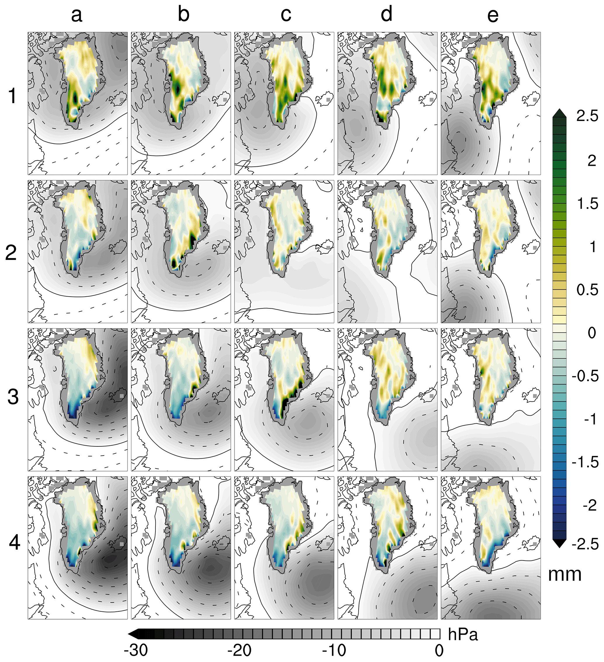
Figure 2Snowfall anomalies over Greenland attributed to common local atmospheric circulation patterns. Snowfall anomaly is relative to the region and annual cycle as identified in Fig. 1, with snowfall from CloudSat observations in units of millimeters per day (mm/d). Local atmospheric circulation patterns were identified using the SOM algorithm, and the low-pressure centers for each circulation pattern are plotted in grey.
To accurately interpret regional circulation patterns in Fig. 2 and their relationship to observations, it is important to understand how the frequency of each pattern changes throughout the year. Here, Fig. 3 shows that the likelihood of occurrence varies intra-annually for each circulation pattern. Figure 3 reveals some general patterns in the annual cycle for the various regional circulation regimes. Southerly transport patterns surrounding node [c,1] occur primarily in summer, with only occasional winter occurrences. The strongest northerly transport patterns surrounding [a,4] occur primarily in winter, with very near zero occurrences during summer months. In contrast, zonal circulation patterns around node [c,3] occur throughout the year. Some individual zonal patterns are more likely to occur in winter or summer depending on cyclone strength and position. The intra-annual variability shown here is consistent with prior regional climatologies (Schuenemann and Cassano, 2010; Mioduszewski et al., 2016).

Figure 3The annual distribution of occurrences of each circulation pattern in Fig. 2 binned by months. Occurrences are counted for all days in the NCEP/NCAR reanalysis from 1948 through 2017. Coloring is used only to visually differentiate months.
4.1 Regional circulation and snowfall variability
Regional snowfall clusters presented in Fig. 1 establish the spatial variability in snowfall across the GrIS and also provide the basis for attributing daily snowfall anomalies to atmospheric circulation. Several notable features of snowfall over Greenland are presented in Fig. 1. The largest snowfall occurs over the southeastern portion of the ice sheet near the coast, with snowfall amounts roughly 5 times more than any other region of the GrIS. While all other regions experience snowfall maxima of approximately 1.0 mm/d in summer or late fall, this southeasterly coastal region reaches a 5.0 mm/d maximum snowfall in January. For regions north of 75∘ latitude, snowfall annual cycle maxima do not exceed 1 mm/d. Of regions north of 75∘, the western coastal regions shown in pink and orange have the highest peak snowfall while regions in the northeast have the lowest.
Relative to these annual cycles, Fig. 2 attributes snowfall anomalies to the daily variability of regional circulation. The southeastern region, a region with a winter snowfall maximum, has the largest anomalous snowfall when cyclone centers are located very near to the southeastern coast. These circulation patterns relate to easterly transport and strong upslope flow against the steep topography of the southeast coast and thus large anomalies tied to orographic forcing. The magnitude of anomalous snowfall in the southeast caused by these easterly patterns is highly dependent on the exact position of the low-pressure center. Circulation patterns [c,3] and [b,2], with cyclones nearest to Greenland's tip, cause the largest snowfall anomalies in this southeastern region. Here, the interaction of this large-scale flow with local fjords, inlets, and peaks leads to distinct enhanced and diminished snowfall dependent on geography.
Over the central GrIS, the largest positive snowfall anomalies relate to southerly transport patterns surrounding node [c,1]. Broad positive snowfall anomalies across the GrIS are seen for circulation patterns where the cyclone center is north of 55∘ latitude and west of the Greenland subcontinent over Baffin Bay. These southerly transport patterns have previously been related to moisture intrusions and atmospheric rivers (Liu and Barnes, 2015; Neff et al., 2014) and are quantified here for the first time in terms of their relationship to the spatial distribution of observed snowfall. For the most prominent of these southerly patterns, node [c,1], anomalously high snowfall extends across the GrIS covering all but the northernmost coastal region.
In regions north of 75∘ latitude on the GrIS, the snowfall anomalies associated with atmospheric circulation are the lowest of anywhere on the GrIS. Positive anomalies on the north and northeastern coast are seen for circulation patterns with cyclone centers above Iceland, in [a,3] and neighboring nodes. These circulation patterns correspond with northerly upslope flow from the Greenland Sea and Arctic Ocean, with snowfall anomalies significantly smaller in both magnitude and spatial extent when compared to snowfall in other GrIS regions.
In order to provide further context for the relationship of snowfall to daily circulation variability, the net snowfall mass input for each SLP circulation pattern was calculated. In this way, Fig. 4 reveals the cumulative snowfall mass input in gigatonnes for each circulation pattern. Unlike Fig. 2, these values are not calculated as anomalies but instead provide the total snowfall mass observed by CloudSat, averaged for each circulation pattern. Thus, Fig. 4 shows cumulative snowfall mass input to the GrIS as described by the daily variability in atmospheric circulation. In contrast to the anomalies shown in Fig. 2, the word cumulative in this text refers to the total magnitude of snowfall for each circulation pattern.
Motivated by the mechanics of GrIS mass changes in the ablation and accumulation zone, Fig. 4a aggregates the cumulative snowfall across the entirety of the GrIS while Fig. 4b includes only observations where surface elevation is above 2 km, and Fig. 4c includes only snowfall observations where surface elevation is below 2 km. Figure 4a is thus the sum of the values presented in Fig. 4b and c. An elevation of 2 km was chosen to delineate the ablation and accumulation zones as previous research has shown that this elevation approximately demarcates the dry region of the GrIS, above which surface melt generally does not occur (McMillan et al., 2016; Hall et al., 2013). This also facilitates comparisons to the GSFC GRACE mass change data product. While the high-resolution spatial variability in snowfall is shown in detail in Fig. 2, Fig. 4 is meant to provide a cumulative value for these spatial characteristics. These quantities are best understood when studied in the spatial context of maps presented in Fig. 2. Values are presented in gigatonnes to facilitate comparisons to the literature and align results presented here with their direct connection to mass balance and thus the fate of the GrIS.
From Fig. 4, the circulation patterns responsible for the largest snowfall mass input to the Greenland ice sheet are southerly transport patterns. Node [c,1] in particular relates to the largest snowfall, with an average daily mass input of 1.66 Gt across the entirety of the GrIS. Figure 4b shows that the majority of this snowfall occurs in the accumulation zone of the GrIS, with 1.2 Gt of the total 1.66 Gt of snowfall occurring over surfaces above 2 km in elevation.
In terms of cumulative snowfall mass input, zonal pattern [c,3] is near the magnitude of these southerly patterns, with a cumulative snowfall mass input of 1.47 Gt, only 10 % less than southerly pattern [c,1]. However, as shown by the spatial snowfall anomalies in Fig. 2 and the cumulative mass input above 2 km of 0.7 Gt from Fig. 4b, the majority of this snowfall occurs on or near the southeastern coast. Also, this particular zonal pattern stands alone in its snowfall impact, as the circulation patterns neighboring [c,3] result in significantly less snowfall mass input. The differences in cumulative snowfall mass input for southerly and zonal circulation patterns are most stark for snowfall above 2 km. Although both southerly pattern [c,1] and zonal pattern [c,3] induce relatively large amounts of snowfall in total, [c,1] transports nearly double the snowfall mass to elevations above 2 km.
Another noteworthy detail of these results is the snowfall impact of circulation pattern [a,1], a broad low-pressure system spanning the GrIS. Figure 4a shows that this pattern results in a significant amount of snowfall, a total of 1.52 Gt, which is near the magnitude of pattern [c,1]. However, the spatial distribution of this snowfall differs significantly, with anomalous snowfall increases on both the southwest and northeastern coasts of the GrIS. As with the zonal circulation pattern [c,3], the northerly transport pattern [a,1] also has a diminished impact on snowfall mass input above 2 km.
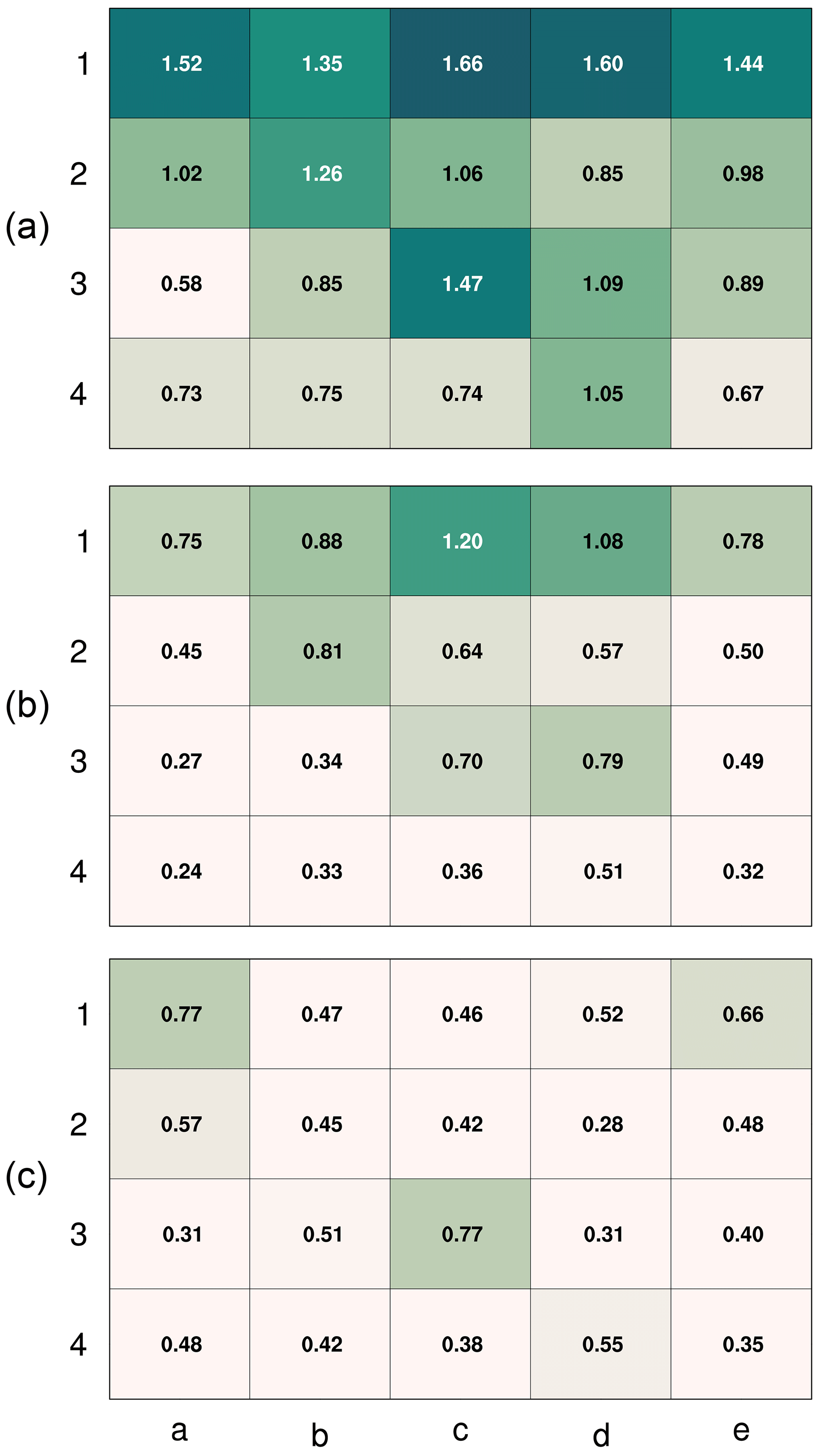
Figure 4(a) The average cumulative snowfall mass (Gt/d) across the entire ice sheet observed by CloudSat for each daily circulation pattern, in gigatonnes. (b) Average total snowfall mass at elevations above 2 km on the GrIS. (c) Average total snowfall mass at elevations below 2 km on the GrIS. The coloring is used only to indicate qualitatively the relative difference in magnitude between patterns.
Quantifying snowfall magnitude and its spatial variability tied to atmospheric circulation provides important information on relationships between the atmosphere, snowfall, and GrIS mass balance. Yet, snowfall is only the mass input to the GrIS. Previous research has examined how atmospheric variability relates to GrIS mass changes (Gallagher et al., 2020; Neff et al., 2014; Fettweis et al., 2011) and concluded that southerly transport, resulting moisture advection, and temperature increases on short timescales contribute significantly to GrIS ablation. These are the same southerly events revealed here to be responsible for the largest snowfall across Greenland. Thus, in the following sections, observations of mass changes are used to quantify the balance between snowfall mass input and net mass changes of the GrIS for this influential southerly regime.
4.2 Circulation, snowfall, and GrIS mass balance changes
4.2.1 Comparing GrIS mass changes from GRACE to CloudSat snowfall
The goal of incorporating observations from GRACE into this analysis is to provide a comparison between the impact of atmospheric circulation on snowfall mass input (Fig. 4) and the actual net mass changes of the GrIS. This is because previous research has demonstrated that the southerly regime, related here to the largest daily snowfall (Fig. 4), corresponds to anomalously warm near-surface temperatures (Gallagher et al., 2020) and melt of the GrIS surface (Mioduszewski et al., 2016). Thus, this section compares GRACE mass changes to the daily snowfall mass variability in Fig. 4 to establish and quantify the relative balance between snowfall and net mass changes for this important southerly circulation regime. Quantifying the balance between southerly circulation, snowfall mass input, and GrIS mass changes in this way provides important insight into the net impact of regional atmospheric variability on the GrIS.
Three figures are provided to examine these relationships. Figure 5 establishes a baseline for comparing GRACE mass changes to the snowfall framework based on regional circulation constructed here. Figure 6 then directly connects mass changes observed above 2 km to pattern [c,1], the circulation pattern related to the largest snowfall. And finally, Fig. 7 improves on Fig. 6 by providing a more statistically robust comparison between occurrences of this important southerly regime and cumulative mass changes of the entire GrIS. The following paragraphs discuss these figures in detail.
First, in Fig. 5, mass changes above 2 km observed by GRACE are directly compared to total monthly snowfall mass values derived from the daily variability of snowfall presented in Fig. 4b. This is done to provide a baseline for comparing the two independent data sources. In Fig. 5, the total snowfall for a given month (x-axis) was constructed by summing the mean snowfall values above 2 km (shown in Fig. 4b) for all circulation patterns occurring in that month. For example, if in July pattern [c,1] occurs 10 times, this would account for a snowfall above 2 km of 12 Gt. Then, if on the remaining 21 d of the month low-snowfall pattern [e,2] occurred averaging snowfall of 0.5 Gt each day, the cumulative snowfall for this July would be Gt.
Thus, the total snowfall mass in a given month can be plotted against the mass change of that month observed by GRACE. In Fig. 5 this comparison is made exclusively in the accumulation zone above 2 km, because, above 2 km, snowfall is the most significant component of mass changes. The other primary component, changes in ice sheet discharge, varies around a mean of 50 Gt/yr (King et al., 2018; Joughin et al., 2018) in the accumulation zone. Variability of ice sheet discharge on monthly timescales is significantly less than the magnitude of snowfall mass input presented here in Fig. 4 (King et al., 2018). Thus, snowfall is the primary driver of GrIS mass changes above 2 km, and circulation patterns related to heavy snowfall can be reliably connected to observations of mass changes in the accumulation region of the GrIS.
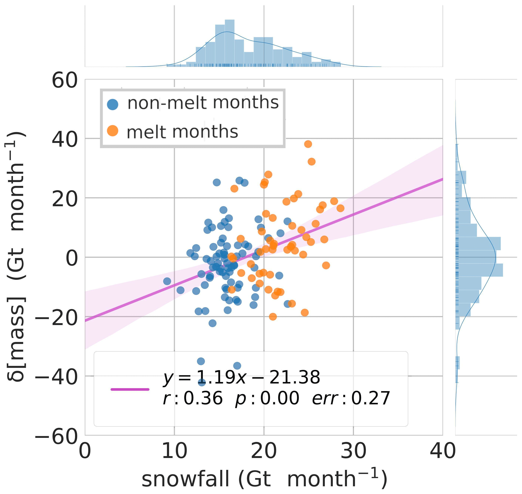
Figure 5A linear regression between the cumulative change in mass above 2 km for a given month as seen by GRACE to the total snowfall mass values summed together for all circulation patterns occurring in that month using daily snowfall mass values related to atmospheric circulation from Fig. 4b. These values are for only the accumulation region of the GrIS above 2 km where snowfall is the primary control on changes in mass. The regression line includes 95 % confidence intervals in transparent red. The regression slope indicates that for every 1.19 Gt of mass change seen by GRACE in a given month there is 1 Gt of snowfall accounted for in Fig. 4b, although with significant variance for individual months. Melt months are highlight in orange and defined to be May, June, July, August, and September. Histograms are proved to characterize the distribution of points
Figure 5 shows that for every 1 Gt of snowfall observed by CloudSat, a corresponding mass change of 1.19 Gt is observed by GRACE in a given month. Despite the significance of this linear regression (p=0.0), an r value of 0.36 indicates a significant amount of variance in the correspondence between the two parameters. While a regression slope of 1.19 is almost 20 % above a perfect correspondence between observations of snowfall and mass changes, a slope of 1.0 is within the 95 % confidence intervals of the regression as a result of the significant variance. This is consistent with other studies finding CloudSat underestimates high-latitude snowfall amounts (Bennartz et al., 2019; Maahn et al., 2014). With consideration for the variance, Fig. 5 demonstrates that the snowfall mass attributed to circulation patterns in Fig. 4b corresponds roughly to mass changes observed by GRACE on monthly timescales.
An important feature of the results in Fig. 5 is the impact of ice sheet dynamics on the intercept of the regression line. While snowfall is the major mass contributor to the GrIS, above 2 km ice sheet dynamics are completely responsible for mass losses. Thus, ice sheet dynamics is a confounding variable in the linear regressions between snowfall and mass changes presented here. To understand this more clearly, projecting the trend from Fig. 5 indicates that in the unrealistic scenario of a month with zero snowfall ice sheet discharge would result in a mass loss of approximately 21 Gt per month in the region of the GrIS above 2 km, with an average snowfall of approximately 17 Gt per month – thus a net mass loss from dynamics of 4 Gt per month or approximately 48 Gt/yr. Also, looking at the confidence intervals on this projection, the bounds on dynamic mass loss above 2 km are likely between ±10 Gt in any given month with extreme months further outside these bounds. In this way, the intra-annual variability of ice sheet dynamics likely explains some of the variability in agreement for individual months in comparing observations of snowfall from CloudSat and mass changes from GRACE.
The variability due to ice sheet dynamics shown here in Fig. 5 mirrors results presented in previous studies. King et al. (2018) showed that dynamic discharge of the northwestern GrIS accounts for an average mass loss of 205 Gt/yr, while Joughin et al. (2018) show that ice velocities in this region average approximately 100 m/yr. Joughin et al. (2018) also show that ice velocities on the central GrIS above 2 km average approximately 25 m/yr, roughly 25 % of the coastal flow velocity. According to these combined studies, mass discharge on the central GrIS would be on the order of 50 Gt/yr using these approximations with inter-annual variability dependent on changes in flow rate. This back-of-the-envelope comparison shows that the comparison presented is physically realistic to first order. However, an accurate estimate of central GrIS flow in terms of mass could not be found in the recent literature. A detailed model of the ice sheet response to snowfall would be required to more deeply explore these results and the variance related to dynamics. With these considerations, Fig. 5 establishes a baseline to compare mass changes observed by GRACE to snowfall mass input derived from CloudSat observations.
4.2.2 Characterizing mass changes in the active southerly circulation regime
Previously cyclones west of Greenland occurring primarily in summer were related to the largest snowfall mass input from CloudSat observations across GrIS. Here this southerly regime is investigated in the full context of GrIS mass changes, including in the ablation region, exploring both mass increases from snowfall as well as characterizing the coinciding mass losses in the ablation region. Because of the findings showing extreme snowfall coinciding with extreme mass loss, this southerly circulation regime is designated the “active” Greenland circulation regime.
Thus, Fig. 6 plots the number of monthly occurrences of circulation pattern [c,1] against the monthly mass deltas observed by GRACE above 2 km observed for that month. Because of the monthly timescale of GRACE observations, mass deltas could not simply be assigned to the daily circulation patterns in Fig. 2. Instead, the relationship between mass changes for each month and the number of occurrences of these southerly circulation patterns are quantified by a linear regression. Accordingly, the linear regression slope indicates the change in mass relative to the number of occurrences of these southerly circulation patterns in a given month. The regressions presented in Fig. 7 were plotted for all circulation patterns in Fig. 2, both individually as well as in groups. The largest regression slope was seen for [c,1], in agreement with the maximum cumulative snowfall above 2 km observed by CloudSat. This approach allows for a direct comparison to CloudSat snow accumulations for circulation patterns presented previously in Fig. 4.
Fig. 6 shows a mass gain in the accumulation region of 1.29 Gt for each occurrence of circulation pattern [c,1], although with significant variability around the regression. While the slope of this regression (1.29 Gt per occurrence) is similar in magnitude to the daily contribution of [c,1] to snowfall mass input in Fig. 4b (1.20 Gt), the relationship is not perfect. A positive slope is only narrowly included in the 95 % confidence interval of the regression, and the p and r values indicate significant variability not constrained by these two parameters. There are three factors that contribute to the significant variance for this regression: (1) natural intra-pattern variability in snowfall for occurrences of each circulation pattern, (2) variability in the circulation patterns co-occurring along with the patterns of interest, and (3) variability in ice sheet dynamics and outflow. Despite this variance, this regression provides further support for the importance of [c,1] to snowfall mass input.

Figure 6A linear regression between the monthly frequency for all occurrences of southerly pattern [c,1] and the cumulative change in mass above 2 km elevation for all months as seen by GRACE. The regression line includes 95 % confidence intervals. Each dot is colored by the time of year that it occurred, with melt months shown in orange defined to be May, June, July, August, and September. The regression line includes 95 % confidence intervals.
Because of the relatively weak statistical correspondence between mass changes and occurrences of pattern [c,1] alone, in Fig. 7 we have combined the three circulation patterns with the largest snowfall. This improves statistics beyond Fig. 6 by sampling a larger number of days in each month. In Fig. 7, mass deltas from GRACE observations are plotted against the number of occurrences of southerly transport patterns [b,1], [c,1], and [d,1] for each month. These plots show monthly GrIS mass changes for all mascons above 2 km (Fig. 7a), below 2 km (Fig. 7b), and for the entire GrIS (Fig. 7c). Comparing mass changes in the accumulation zone from Fig. 7a with snowfall in Fig. 4b, the snowfall mass input of the three patterns averages 1.05 Gt, while a cumulative mass change of 0.96 Gt is observed by GRACE for each occurrence of these three patterns, with some variance. This shows, within the significant measurement uncertainties, that GRACE observations correspond with the mass changes caused by snowfall in the accumulation zone.
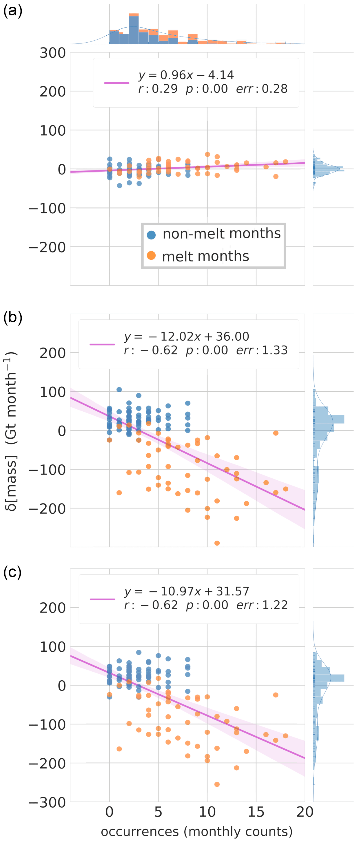
Figure 7A linear regression, as in Fig. 6, but for all occurrences of southerly patterns [b,1], [c,1], and [d,1]. The regression line includes 95 % confidence intervals. Each dot is colored by the time of year that it occurred, with melt months defined to be May, June, July, August, and September. (a) Mass change for GRACE mascons above 2 km. (b) Mass change for GRACE mascons below 2 km. (c) Mass change for all Greenland GRACE mascons, both above and below 2 km.
Comparing the mass changes in the ablation and accumulation regions of the ice sheet in Fig. 7, the relative magnitude of mass loss and snowfall for these southerly events can be assessed. In Fig. 7a, the regression slope describes a relationship where GrIS mass above 2 km increases 0.96 Gt for each occurrence of these southerly transport patterns, with a similar relationship observed year-round in this typically non-melting region. Conversely, below 2 km on the GrIS, the linear regression for all months in Fig. 7b indicates that mass decreases 12.02 Gt for each occurrence of these southerly patterns. It is worth noting that when considering only the non-melt months, linear regression indicates that mass increases by 2.2 Gt for each additional occurrence of the southerly patterns, providing a reasonable sanity check on this methodology. When considering the whole GrIS over all months (Fig. 7c), coastal ablation is an order of magnitude larger than snowfall mass increases, leading to a net mass loss of 10.97 Gt across the entire ice sheet for each occurrence of southerly circulation patterns, showing that for these patterns mass loss from ablation is significantly larger than snowfall mass input. Again, for only the winter months over the full GrIS, the methodology suggests a net mass increase of 2.2 Gt per occurrence of southerly patterns. Combined together, Figs. 5, 6, and 7 are intended to support the discussion and conclusions based on the relative proportions of snowfall mass input and GrIS ablation as well as provide a baseline for understanding snowfall in the broader context of GrIS mass changes.
To put this mass loss from ablation in the context of the atmospheric circulation framework used here, NCEP/NCAR reanalysis daily mean temperatures were related to the circulation patterns shown in Fig. 2. Figure 8 shows the mean daily position of the zero-degree isotherm for occurrences of each circulation pattern. Although the zero-degree isotherm position is dependent on the seasonal fraction of occurrence of each pattern, it provides a simple proxy to understand how circulation patterns presented here relate to GrIS ablation processes. The discussion of ablation here is supported by a more detailed analysis of temperature, cloud impacts, and atmospheric circulation patterns found in Gallagher et al. (2020), as well as other literature detailing the atmospheric contribution to ablation processes (Neff et al., 2014; Hanna et al., 2014; Fettweis et al., 2011; Mioduszewski et al., 2016).
The relationship between atmospheric circulation and warm temperatures on the GrIS in Fig. 8 illustrates the connection between southerly transport and broad warming. Southerly circulation patterns surrounding node [c,1] relate to the largest fractions of the GrIS with temperatures above 0 ∘C. In the context of the snowfall results presented at the beginning of this paper, these southerly transport patterns are thus the most active atmospheric regimes in terms of their impact on daily variability in GrIS mass balance. Node [c,1] in particular relates to the largest daily snowfall mass input of any circulation pattern at 1.66 Gt as well as the largest broad warming above 0 ∘C and resulting melt as supported by Mioduszewski et al. (2016). However, the relative magnitude of these co-occurring and competing impacts on mass balance had not previously been quantified. In this way, Fig. 7 provides an estimate of the balance between ablation and accumulation, showing that mass loss in the ablation zone is significantly larger than snowfall for occurrences of this southerly regime.
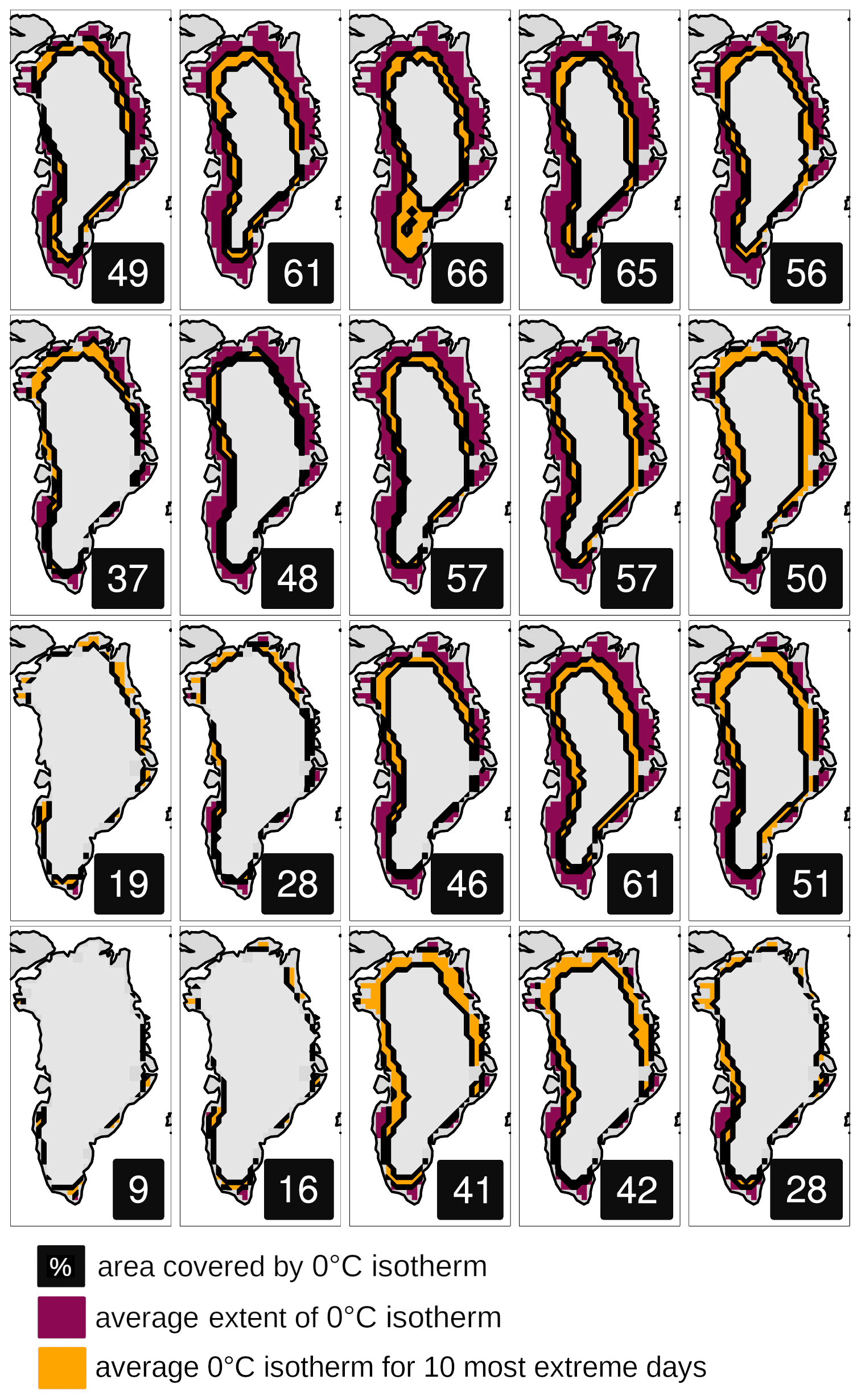
Figure 8The average position of the zero-degree isotherm for all days associated with each circulation pattern. Data are from gridded NCEP/NCAR reanalysis fields of 2 m temperatures for the entire NCEP/NCAR reanalysis record from 1948 through 2017. Red coloring shows the mean position of the zero-degree isotherm for all days for the full set of reanalysis data. Orange coloring indicates the position of the zero-degree isotherm for only the 10 warmest days during the CloudSat data period from 2006–2011. The numbers in the black box indicate the percentage of the total area of the GrIS covered by the orange region for these 10 most extreme days.
While a large portion of this paper has focused on the atmospheric drivers of large snowfall events and their relationship to ablation, these events occur on relatively short timescales, most often in summer. In the framework of this paper, other relationships between snowfall and atmospheric circulation can also be discussed. In opposition to these southerly events most frequent in summer, these results show that circulation patterns surrounding [a,4] related to northerly transport occur most frequently in winter. Despite their nominal snowfall, these northerly patterns occur primarily in winter when GrIS ablation is at a minimum and thus relate to consistent mass increases. In this way, these results show that moderate snowfall in winter relates to the largest mass increases on long-term timescales, in agreement with prior research (Koenig et al., 2016). Although the focus here is primarily on the so-called “active” southerly circulation regime, the analysis, methodology, and figures provide context for the complete variability in local atmospheric state. To keep the written discussion from being even more verbose, further detailed understanding of these patterns may be gleaned from the graphical figures.
4.2.3 Discussion of uncertainty
While this work brings to light new understanding, assessing the potential uncertainty in the results is as important as it is difficult. The primary conclusions of the paper are motivated by the snowfall anomaly calculations made using CloudSat observations aggregated in spatial clusters and then processed via spectral analysis. Propagating the statistical uncertainty through this machinery would be Herculean in effort as well as difficult to interpret scientifically. Thus, in lieu of being able to directly quantify the resulting uncertainty, we will instead discuss the validity of using these observations as inputs for these methods.
While individual snowfall observations retrieved from CloudSat profiles have large uncertainties, observations averaged in time have been shown to compare very accurately to surface in situ measurements of snowfall measurements over Greenland (Bennartz et al., 2019; Boening et al., 2012). In this way, this analysis uses the aggregated mean of a large sample of observations: the mean snowfall rate is sampled from many CloudSat profiles across a 1×1∘ pixel which is then averaged for the locally clustered region to create the seasonal background variability, which is in turn used to calculate the anomaly for the average of all snowfall observations for a given circulation pattern. Thus, any particular anomaly value plotted in Fig. 2 is the average of many hundreds of snowfall observations, while the cumulative GrIS snowfall mass input values from Fig. 4 are the average of many thousands – the conclusion being that the significant uncertainty and noise in individual observations will be largely canceled by the processing. This is evidenced by the relatively smooth transitions in the spatial snowfall anomalies driven by circulation (Fig. 2), indicating that the pixel-by-pixel noise is significantly lower than the observation signal.
For the GRACE component of the analysis, much like CloudSat snowfall observations, the uncertainty of any individual mass delta observation for a particular mascon is very high, due primarily to the noise present in the GRACE measurement system (Luthcke et al., 2013). Further, previous research has also shown that for averaging mascon observations across large areas of the GrIS uncertainty contributions from noise are largely negligible (Ran et al., 2017). For the analysis presented here, monthly mass changes are averaged for two distinct large areas of the GrIS above and below 2 km. As a result, the significant uncertainty resulting from noise in GRACE measurements is minimized for this analysis.
These paragraphs are the attempt of the authors to acknowledge there are many factors at play in presenting a comparison between such disparate datasets using relatively complex methodologies. Although the very close agreement in mass changes is extremely compelling, the analysis is most compelling for the fact that the results provide new detailed information about key GrIS processes, leading to conclusions that can be scientifically reasoned with.
By combining CloudSat snowfall observations together with a classification of atmospheric circulation, this paper constructs a spatial relationship between snowfall and the mass balance of the GrIS on daily timescales. To contextualize these results in terms of GrIS mass balance more broadly, GRACE observations were utilized to show how snowfall mass input relates to net mass changes.
The snowfall observations presented here show that snow input peaks for the majority of the GrIS in the mid-to-late summer months. Further, summer snowfall is shown to be 2 to 4 times greater in magnitude than snowfall in winter, with the inter-annual variability in snowfall relating to the seasonal variability in occurrence of specific circulation patterns. These findings confirm previous studies (Bennartz et al., 2019) and bring further context. Mapping the spatial variability in snowfall to these regional circulation patterns shows that snowfall across Greenland relates closely to the position and strength of cyclonic systems, with localized snowfall closely tied to the location of onshore atmospheric flow. More specifically, the southerly transport regime with cyclones west of the GrIS, most commonly occurring in summer, is implicated in the largest snowfall both in mass input and spatial extent. More specifically, for the most prominent southerly circulation pattern, daily snowfall mass input across Greenland is a total of 1.66 Gt. Spatially, this southerly circulation regime is the primary source of snowfall on the central ice sheet as with 1.2 Gt of the total 1.66 Gt falling in the accumulation zone above 2 km elevation.
Observations of mass changes from GRACE independently show that these same primarily summer southerly circulation patterns also relate to significant mass loss in the ablation zone of the GrIS. Thus, the southerly regime has been designated the “active” circulation regime due to the quantified relationships between large snowfall mass input coinciding with significant mass loss. While the snowfall for this southerly regime averages between 1.3 and 1.6 Gt per day, GRACE observations implicate this southerly pattern in a mass loss on the order of 11 Gt per each daily occurrence.
More generally, across Greenland daily snowfall mass input varies between 0.58 and 1.66 Gt, depending on the atmospheric circulation conditions for a particular day. Above 2 km in the accumulation region there is even higher variability in daily snowfall mass input. In the accumulation zone the largest snowfall results from southerly transport with a maximum of 1.20 Gt relating to daily occurrences of pattern [c,1]. This is in comparison to northerly events that contribute as little as 0.24 Gt of snowfall to the central ice sheet. These results provide a new constraint on the daily spatial variability of snowfall mass input across Greenland using direct observations of snowfall.
Resulting from the novel combined methodologies presented in this paper, a direct comparison between GRACE observations and the aggregated results of snowfall mass input is presented. Through this comparison it is shown that observations from GRACE of mass change approximately agree in magnitude with the aggregated results from CloudSat snowfall. For the methodology presented here, every 1.0 Gt of snowfall mass input observed by CloudSat corresponded with a mass increase observed by GRACE of 1.19 Gt, an approximately 20 % underestimation of snowfall mass input using aggregated CloudSat observations. While imperfect, the agreement between these independent observations provides compelling evidence in favor of the methodologies presented, particularly considering the disparate nature of CloudSat and GRACE observations. This disagreement is also within the uncertainty of the observations and approximately near the magnitude of previously reported tendencies for CloudSat to underestimate snowfall in the Arctic (Bennartz et al., 2019; Maahn et al., 2014).
The work presented in this paper provides new insight, rooted in observations, into the relationships between broader atmospheric conditions, spatial snowfall variability across Greenland, and corresponding GrIS mass changes. Further, because this novel methodology constructs never-before-seen maps of the daily spatial variability of snowfall across Greenland, the authors hope that this work will lead to more accurate research of snowfall and accumulation processes across Greenland, with potential applications investigating detailed process models, climate projections, and paleoclimate studies. In the future warmer wetter Arctic (Boisvert and Stroeve, 2015; Schuenemann and Cassano, 2010), changes in the relationship between snowfall and GrIS mass balance may significantly alter the relationships analyzed here. Modeling the evolution of snowfall mass input forward in time would be one way to contextualize these new results more broadly in the uncertain future of GrIS mass balance.
All data products used in this study are available on the web from the primary sources cited in the acknowledgements. All code is available on request from the authors.
MRG designed the methodology, performed the analyses, and wrote the manuscript. MDS contributed to the methodology development, scientific feedback, and the writing and editing of the manuscript. HC contributed remote sensing expertise, contributed scientific feedback, and participated in the production of the manuscript. TL contributed feedback on CloudSat precipitation interpretation, helped with the processing of these data, and provided scientific feedback. All authors commented on and approved of this paper.
The contact author has declared that neither they nor their co-authors have any competing interests.
Publisher’s note: Copernicus Publications remains neutral with regard to jurisdictional claims in published maps and institutional affiliations.
This research was supported by the National Science Foundation grants PLR-1303879, OPP-1801477, and PLR-1314156, as well as the NOAA Physical Sciences Laboratory. We thank the Laboratoire de Météorologie Dynamique for their support and funding of international collaboration for this work. We kindly thank Jen Kay for her support and feedback on topics in this paper. GRACE Mass Variability Time Series were obtained from NASA's GSFC GRACE mascon solutions at https://neptune.gsfc.nasa.gov/gngphys/index.php?section=470 (last access: September 2020). CloudSat observations were obtained from the CloudSat Data Center at https://www.cloudsat.cira.colostate.edu/ (last access: September 2020). NCEP/NCAR reanalysis data were obtained from the NOAA Physical Science Laboratory in Boulder, Colorado, USA (https://psl.noaa.gov/, last access: September 2020). The authors would also like to acknowledge the many incredible free and open-source computing tools that have made this work possible, including but not limited to Arch (GNU/)Linux, Emacs, NCL, Python, and the following packages: pandas, scipy, numpy, matplotlib, and scikit-learn. The work in this paper is dedicated to the memory of Mike Wilson, an incredible person who did not just teach high school science but taught lessons in how to be a curious person. Mike Wilson, your caring will not be forgotten.
This research has been supported by the National Science Foundation (grant nos. PLR-1303879, OPP-1801477, and PLR-1314156).
This paper was edited by Ruth Mottram and reviewed by two anonymous referees.
Bennartz, R., Fell, F., Pettersen, C., Shupe, M. D., and Schuettemeyer, D.: Spatial and temporal variability of snowfall over Greenland from CloudSat observations, Atmos. Chem. Phys., 19, 8101–8121, https://doi.org/10.5194/acp-19-8101-2019, 2019. a, b, c, d, e, f, g
Boening, C., Lebsock, M., Landerer, F., and Stephens, G.: Snowfall-driven mass change on the East Antarctic ice sheet, Geophys. Res. Lett., 39, 1–5, https://doi.org/10.1029/2012GL053316, 2012. a
Boisvert, L. N. and Stroeve, J. C.: The Arctic is becoming warmer and wetter as revealed by the Atmospheric Infrared Sounder, Geophys. Res. Lett., 42, 4439–4446, https://doi.org/10.1002/2015GL063775, 2015. a
Box, J. E., Bromwich, D. H., Veenhuis, B. A., Bai, L.-S., Stroeve, J. C., Rogers, J. C., Steffen, K., Haran, T., and Wang, S.-H.: Greenland Ice Sheet Surface Mass Balance Variability (1988–2004) from Calibrated Polar MM5 Output, J. Climate, 19, 2783–2800, https://doi.org/10.1175/JCLI3738.1, 2006. a
Cao, Q., Zhang, J., Gourley, J. J., Kirstetter, P. E., Chen, S., and Hong, Y.: Snowfall Detectability of Nasa'S Cloudsat: the First Cross-Investigation of Its 2C-Snow-Profile Product and National Multi-Sensor Mosaic Qpe (Nmq) Snowfall Data, Prog. Electromagn. Res., 148, 55–61, https://doi.org/10.2528/pier14030405, 2014. a
Crane, R. G. and Hewitson, B. C.: Clustering and upscaling of station precipitation records to regional patterns using self-organizing maps (SOMs), Clim. Res., 25, 95–107, https://doi.org/10.3354/cr025095, 2003. a
Danco, J. F., DeAngelis, A. M., Raney, B. K., and Broccoli, A. J.: Effects of a Warming Climate on Daily Snowfall Events in the Northern Hemisphere, J. Climate, 29, 6295–6318, https://doi.org/10.1175/JCLI-D-15-0687.1, 2016. a
Doyle, S. H., Hubbard, A., Van De Wal, R. S., Box, J. E., Van As, D., Scharrer, K., Meierbachtol, T. W., Smeets, P. C., Harper, J. T., Johansson, E., Mottram, R. H., Mikkelsen, A. B., Wilhelms, F., Patton, H., Christoffersen, P., and Hubbard, B.: Amplified melt and flow of the Greenland ice sheet driven by late-summer cyclonic rainfall, Nat. Geosci., 8, 647–653, https://doi.org/10.1038/ngeo2482, 2015. a
Edel, L., Claud, C., Genthon, C., Palerme, C., Wood, N., L’Ecuyer, T., and Bromwich, D.: Arctic Snowfall from CloudSat Observations and Reanalyses, J. Climate, 33, 2093–2109, https://doi.org/10.1175/JCLI-D-19-0105.1, 2020. a
Fettweis, X., Mabille, G., Erpicum, M., Nicolay, S., and van den Broeke, M.: The 1958-2009 Greenland ice sheet surface melt and the mid-tropospheric atmospheric circulation, Clim. Dynam., 36, 139–159, https://doi.org/10.1007/s00382-010-0772-8, 2011. a, b
Gallagher, M., Shupe, M. D., and Miller, N. B.: Impact of Atmospheric Circulation on Temperature, Clouds, and Radiation at Summit Station, Greenland with Self-Organizing Maps, J. Climate, 31, 8895–8915, https://doi.org/10.1175/JCLI-D-17-0893.1, 2018. a, b, c
Gallagher, M. R., Chepfer, H., Shupe, M. D., and Guzman, R.: Warm Temperature Extremes Across Greenland Connected to Clouds, Geophys. Res. Lett., 47, e2019GL086059, https://doi.org/10.1029/2019GL086059, 2020. a, b, c, d, e
Hall, D. K., Comiso, J. C., Digirolamo, N. E., Shuman, C. A., Box, J. E., and Koenig, L. S.: Variability in the surface temperature and melt extent of the Greenland ice sheet from MODIS, Geophys. Res. Lett., 40, 2114–2120, https://doi.org/10.1002/grl.50240, 2013. a
Hanna, E., Fettweis, X., Mernild, S. H., Cappelen, J., Ribergaard, M. H., Shuman, C. A., Steffen, K., Wood, L., and Mote, T. L.: Atmospheric and oceanic climate forcing of the exceptional Greenland ice sheet surface melt in summer 2012, Int. J. Climatol., 34, 1022–1037, https://doi.org/10.1002/joc.3743, 2014. a
Hewitson, B. C. and Crane, R. G.: Self-organizing maps : applications to synoptic climatology, Clim. Res., 22, 13–26, 2002. a
Im, E., Wu, C., and Durden, S. L.: Cloud profiling radar for the CloudSat mission, IEEE National Radar Conference – Proceedings, 2005-Janua, 483–486, https://doi.org/10.1109/RADAR.2005.1435874, 2005. a
Joughin, I., Smith, B. E., and Howat, I.: Greenland Ice Mapping Project: ice flow velocity variation at sub-monthly to decadal timescales, The Cryosphere, 12, 2211–2227, https://doi.org/10.5194/tc-12-2211-2018, 2018. a, b, c
Kalnay, E., Kanamitsu, M., Kistler, R., Collins, W., Deaven, D., Gandin, L., Iredell, M., Saha, S., White, G., Woollen, J., Zhu, Y., Leetmaa, A., Reynolds, R., Chelliah, M., Ebisuzaki, W., Higgins, W., Janowiak, J., Mo, K. C., Ropelewski, C., Wang, J., Jenne, R., and Joseph, D.: The NCEP/NCAR 40-year reanalysis project, B. Am. Meteorol. Soc., 77, 437–471, https://doi.org/10.1175/1520-0477(1996)077<0437:TNYRP>2.0.CO;2, 1996. a
King, M. D., Howat, I. M., Jeong, S., Noh, M. J., Wouters, B., Noël, B., and van den Broeke, M. R.: Seasonal to decadal variability in ice discharge from the Greenland Ice Sheet, The Cryosphere, 12, 3813–3825, https://doi.org/10.5194/tc-12-3813-2018, 2018. a, b, c
Koenig, L. S., Ivanoff, A., Alexander, P. M., MacGregor, J. A., Fettweis, X., Panzer, B., Paden, J. D., Forster, R. R., Das, I., McConnell, J. R., Tedesco, M., Leuschen, C., and Gogineni, P.: Annual Greenland accumulation rates (2009–2012) from airborne snow radar, The Cryosphere, 10, 1739–1752, https://doi.org/10.5194/tc-10-1739-2016, 2016. a
Kohonen, T.: Essentials of the self-organizing map, Neural Networks, 37, 52–65, https://doi.org/10.1016/j.neunet.2012.09.018, 2013. a
Liu, C. and Barnes, E. A.: Extrememoisture transport into the Arctic linked to Rossby wave breaking, J. Geophys. Res., 120, 3774–3788, https://doi.org/10.1002/2014JD022796, 2015. a
Luthcke, S. B., Camp, J., Arendt, A., Loomis, B., Sabaka, T., and McCarthy, J.: Antarctica, Greenland and Gulf of Alaska land-ice evolution from an iterated GRACE global mascon solution, J. Glaciol., 59, 613–631, https://doi.org/10.3189/2013jog12j147, 2013. a, b
Maahn, M., Burgard, C., Crewell, S., Gorodetskaya, I. V., Kneifel, S., Lhermitte, S., Van Tricht, K., and Van Lipzig, N. P.: How does the spaceborne radar blind zone affect derived surface snowfall statistics in polar regions?, J. Geophys. Res., 119, 13604–13620, https://doi.org/10.1002/2014JD022079, 2014. a, b, c
Mattingly, K. S., Mote, T. L., and Fettweis, X.: Atmospheric River Impacts on Greenland Ice Sheet Surface Mass Balance, J. Geophys. Res.-Atmos., 123, 8538–8560, https://doi.org/10.1029/2018JD028714, 2018. a
McIlhattan, E. A., Pettersen, C., Wood, N. B., and L'Ecuyer, T. S.: Satellite observations of snowfall regimes over the Greenland Ice Sheet, The Cryosphere, 14, 4379–4404, https://doi.org/10.5194/tc-14-4379-2020, 2020. a
McMillan, M., Leeson, A., Shepherd, A., Briggs, K., Armitage, T. W. K., Hogg, A., Kuipers Munneke, P., van den Broeke, M., Noël, B., van de Berg, W. J., Ligtenberg, S., Horwath, M., Groh, A., Muir, A., and Gilbert, L.: A high-resolution record of Greenland mass balance, Geophys. Res. Lett., 43, 7002–7010, https://doi.org/10.1002/2016GL069666, 2016. a
Mioduszewski, J. R., Rennermalm, A. K., Hammann, A., Tedesco, M., Noble, E. U., Stroeve, J. C., and Mote, T. L.: Atmospheric drivers of Greenland surface melt revealed by self-organizing maps, J. Geophys. Res.-Atmos., 121, 5095–5114, https://doi.org/10.1002/2015JD024550, 2016. a, b, c, d, e
Neff, W., Compo, G. P., Martin Ralph, F., and Shupe, M. D.: Continental heat anomalies and the extreme melting of the Greenland ice surface in 2012 and 1889, J. Geophys. Res.-Atmos., 119, 6520–6536, https://doi.org/10.1002/2014JD021470, 2014. a, b, c, d
Noël, B., van de Berg, W. J., van Meijgaard, E., Kuipers Munneke, P., van de Wal, R. S. W., and van den Broeke, M. R.: Evaluation of the updated regional climate model RACMO2.3: summer snowfall impact on the Greenland Ice Sheet, The Cryosphere, 9, 1831–1844, https://doi.org/10.5194/tc-9-1831-2015, 2015. a, b
Norin, L., Devasthale, A., L'Ecuyer, T. S., Wood, N. B., and Smalley, M.: Intercomparison of snowfall estimates derived from the CloudSat Cloud Profiling Radar and the ground-based weather radar network over Sweden, Atmos. Meas. Tech., 8, 5009–5021, https://doi.org/10.5194/amt-8-5009-2015, 2015. a
Pedersen, S. H., Tamstorf, M. P., Abermann, J., Lund, M., Skov, K., Sigsgaard, C., Mylius, M. R., Hansen, B. U., Liston, G. E., Schmidt, N. M., Højlund, S., Tamstorf, M. P., Abermann, J., Pedersen, S. H., Tamstorf, M. P., Abermann, J., Westergaard-nielsen, A., Lund, M., Skov, K., Sigsgaard, C., Mylius, M. R., Hansen, B. U., Liston, G. E., and Schmidt, N. M.: Spatiotemporal Characteristics of Seasonal Snow Cover in Northeast Greenland from in Situ Observations Spatiotemporal characteristics of seasonal snow cover in Northeast Greenland from in situ observations, Arct. Antarct. Alp. Res., 48, 653–671, https://doi.org/10.1657/AAAR0016-028, 2018. a
Pedregosa, F., Varoquaux, G., Gramfort, A., Michel, V., Thirion, B., Grisel, O., Blondel, M., Prettenhofer, P., Weiss, R., Dubourg, V., Vanderplas, J., Passos, A., Cournapeau, D., Brucher, M., Perrot, M., and Duchesnay, E.: Scikit-learn: Machine Learning in Python, J. Mach. Learn. Res., 12, 2825–2830, 2011. a
Pettersen, C., Bennartz, R., Merrelli, A. J., Shupe, M. D., Turner, D. D., and Walden, V. P.: Precipitation regimes over central Greenland inferred from 5 years of ICECAPS observations, Atmos. Chem. Phys., 18, 4715–4735, https://doi.org/10.5194/acp-18-4715-2018, 2018. a, b
Ran, J., Ditmar, P., Klees, R., and Farahani, H. H.: Statistically optimal estimation of Greenland Ice Sheet mass variations from GRACE monthly solutions using an improved mascon approach, J. Geodesy, 92, 299–319, https://doi.org/10.1007/s00190-017-1063-5, 2017. a
Ryan, J. C., Smith, L. C., Wu, M., Cooley, S. W., Miège, C., Montgomery, L. N., Koenig, L. S., Fettweis, X., Noel, B. P. Y., and van den Broeke, M. R.: Evaluation of CloudSat’s Cloud-Profiling Radar for Mapping Snowfall Rates Across the Greenland Ice Sheet, J. Geophys. Res.-Atmos., 125, e2019JD031411, https://doi.org/10.1029/2019JD031411, 2020. a, b
Schuenemann, K. C. and Cassano, J. J.: Changes in synoptic weather patterns and Greenland precipitation in the 20th and 21st centuries: 2. Analysis of 21st century atmospheric changes using self-organizing maps, J. Geophys. Res.-Atmos., 115, 1–18, https://doi.org/10.1029/2009JD011706, 2010. a, b, c, d, e
Shepherd, A., Ivins, E. R., A, G., Barletta, V. R., Bentley, M. J., Bettadpur, S., Briggs, K. H., Bromwich, D. H., Forsberg, R., Galin, N., Horwath, M., Jacobs, S., Joughin, I., King, M. A., Lenaerts, J. T. M., Li, J., Ligtenberg, S. R. M., Luckman, A., Luthcke, S. B., McMillan, M., Meister, R., Milne, G., Mouginot, J., Muir, A., Nicolas, J. P., Paden, J., Payne, A. J., Pritchard, H., Rignot, E., Rott, H., Sorensen, L. S., Scambos, T. A., Scheuchl, B., Schrama, E. J. O., Smith, B., Sundal, A. V., van Angelen, J. H., van de Berg, W. J., van den Broeke, M. R., Vaughan, D. G., Velicogna, I., Wahr, J., Whitehouse, P. L., Wingham, D. J., Yi, D., Young, D., and Zwally, H. J.: A Reconciled Estimate of Ice-Sheet Mass Balance, Science, 338, 1183–1189, https://doi.org/10.1126/science.1228102, 2012. a
Sheridan, S. C. and Lee, C. C.: The self-organizing map in synoptic climatological research, Prog. Phys. Geogr., 35, 109–119, https://doi.org/10.1177/0309133310397582, 2011. a
Stephens, G., Winker, D., Pelon, J., Trepte, C., Vane, D., Yuhas, C., L'Ecuyer, T., and Lebsock, M.: Cloudsat and calipso within the a-train: Ten years of actively observing the earth system, B. Am. Meteorol. Soc., 99, 569–581, https://doi.org/10.1175/BAMS-D-16-0324.1, 2018. a
Stephens, G. L., Vane, D. G., Tanelli, S., Im, E., Durden, S., Rokey, M., Reinke, D., Partain, P., Mace, G. G., Austin, R., L'Ecuyer, T., Haynes, J., Lebsock, M., Suzuki, K., Waliser, D., Wu, D., Kay, J., Gettelman, A., Wang, Z., and Marchand, R.: CloudSat mission: Performance and early science after the first year of operation, J. Geophys. Res.-Atmos., 114, 1–18, https://doi.org/10.1029/2008JD009982, 2008. a
van den Broeke, M. R., Bamber, J. L., Ettema, J., Rignot, E. J., Schrama, E., van de Berg, W. J., van Meijgaard, E., Velicogna, I., Wouters, B., Broeke, M. V. D., Bamber, J. L., Ettema, J., Rignot, E. J., Schrama, E., Berg, W. J. V. D., Meijgaard, E. V., Velicogna, I., and Wouters, B.: Partitioning Recent Greenland Mass Loss, Science, 326, 984–986, https://doi.org/10.1126/science.1178176, 2009. a
van den Broeke, M. R., Enderlin, E. M., Howat, I. M., Kuipers Munneke, P., Noël, B. P. Y., van de Berg, W. J., van Meijgaard, E., and Wouters, B.: On the recent contribution of the Greenland ice sheet to sea level change, The Cryosphere, 10, 1933–1946, https://doi.org/10.5194/tc-10-1933-2016, 2016. a
Vernon, C. L., Bamber, J. L., Box, J. E., van den Broeke, M. R., Fettweis, X., Hanna, E., and Huybrechts, P.: Surface mass balance model intercomparison for the Greenland ice sheet, The Cryosphere, 7, 599–614, https://doi.org/10.5194/tc-7-599-2013, 2013. a
Wood, N. B. and L'Ecuyer, T. S.: What millimeter-wavelength radar reflectivity reveals about snowfall: an information-centric analysis, Atmos. Meas. Tech., 14, 869–888, https://doi.org/10.5194/amt-14-869-2021, 2021. a
Wood, N. B., L'Ecuyer, T. S., Bliven, F. L., and Stephens, G. L.: Characterization of video disdrometer uncertainties and impacts on estimates of snowfall rate and radar reflectivity, Atmos. Meas. Tech., 6, 3635–3648, https://doi.org/10.5194/amt-6-3635-2013, 2013. a
Wood, N. B., L'Ecuyer, T. S., Heymsfield, A. J., Stephen, G. L., Hudak, D. R., and Rodriguez, P.: Estimating snow microphysical properties using collocated multisensor observations, J. Geophys. Res., 119, 8941–8961, https://doi.org/10.1002/2013JD021303, 2014. a