the Creative Commons Attribution 4.0 License.
the Creative Commons Attribution 4.0 License.
 | 25 Aug 2022
Cloud forcing of surface energy balance from in situ measurements in diverse mountain glacier environments
Jonathan P. Conway
Jakob Abermann
Liss M. Andreassen
Mohd Farooq Azam
Nicolas J. Cullen
Noel Fitzpatrick
Rianne H. Giesen
Kirsty Langley
Shelley MacDonell
Thomas Mölg
Valentina Radić
Carleen H. Reijmer
Jean-Emmanuel Sicart
Clouds are an important component of the climate system, yet our understanding of how they directly and indirectly affect glacier melt in different climates is incomplete. Here we analyse high-quality datasets from 16 mountain glaciers in diverse climates around the globe to better understand how relationships between clouds and near-surface meteorology, radiation and surface energy balance vary. The seasonal cycle of cloud frequency varies markedly between mountain glacier sites. During the main melt season at each site, an increase in cloud cover is associated with increased vapour pressure and relative humidity, but relationships to wind speed are site specific. At colder sites (average near-surface air temperature in the melt season <0 ∘C), air temperature generally increases with increasing cloudiness, while for warmer sites (average near-surface air temperature in the melt season ≫0 ∘C), air temperature decreases with increasing cloudiness. At all sites, surface melt is more frequent in cloudy compared to clear-sky conditions. The proportion of melt from temperature-dependent energy fluxes (incoming longwave radiation, turbulent sensible heat and latent heat) also universally increases in cloudy conditions. However, cloud cover does not affect daily total melt in a universal way, with some sites showing increased melt energy during cloudy conditions and others decreased melt energy. The complex association of clouds with melt energy is not amenable to simple relationships due to many interacting physical processes (direct radiative forcing; surface albedo; and co-variance with temperature, humidity and wind) but is most closely related to the effect of clouds on net radiation. These results motivate the use of physics-based surface energy balance models for representing glacier–climate relationships in regional- and global-scale assessments of glacier response to climate change.
- Article
(12115 KB) - Full-text XML
- BibTeX
- EndNote


Mountain glaciers are sensitive and important components of the climate system. Over the last 50 years, mountain glacier melt has contributed 36 %–40 % of the observed global sea level rise (Hock et al., 2009; Church et al., 2011; Mernild et al., 2014; Zemp et al., 2019; Hugonnet et al., 2021). During the rest of the 21st century, a large but uncertain fraction of the remaining mass stored in mountain glaciers is expected to melt (Radić et al., 2014; Kraaijenbrink et al., 2017; Marzeion et al., 2018; Huss and Hock, 2018; Zekollari et al., 2019). As glaciers are sensitive to change in their surrounding climate, they can be used to infer past changes in climate over decadal (e.g. Mackintosh et al., 2017), centennial (e.g. Oerlemans, 2005; Mölg et al., 2009b) and paleo-climatic timescales (e.g. Putnam et al., 2012).
Our ability to determine how mountain glacier melt responds to changes in climate depends on the ability of models to correctly represent the processes that occur at the atmosphere–glacier interface and link near-surface meteorology and surface melt. The surface energy balance (SEB) is the key process that controls the rate of melt at the glacier surface and can be represented as
where QM is the energy available for melt (zero when surface is freezing), SWnet and LWnet are the net fluxes of shortwave and longwave radiation (including shortwave radiation that penetrates the surface), QS and QL are the turbulent fluxes of sensible and latent heat, QC is the heat flux at the surface from conduction within the glacier, and QPRC is the heat advected from precipitation. All fluxes are given in watts per square metre (W m−2) , and those on the righthand side of Eq. (1) are defined as positive towards the surface. When the surface is at the melting point (i.e. surface temperature (Ts)=0 ∘C), QM becomes non-zero and positive, and surface melt (M, mm water equivalent) is determined through
where Δt is the time step of model output (seconds) and Lf is the latent heat of fusion (3.34×10⁵ J kg−1). In many studies, these relationships between near-surface meteorology and melt are simplified into parameterisations that require less input data such as temperature index or enhanced temperature index melt models (Huybrechts and Oerlemans, 1990; Hock, 2003; Pellicciotti et al., 2005).
While we know that glaciers are sensitive to changes in local climate, the extent to which cloud cover will amplify or reduce the melting of a glacier in response to future atmospheric warming is uncertain. Clouds alter the incoming shortwave (SWin) and longwave (LWin) radiation, which are generally the largest sources of energy at the glacier surface (Sicart et al., 2008; Pellicciotti et al., 2011; Van Den Broeke et al., 2011; Cullen and Conway, 2015). Over highly reflective glacier surfaces (e.g. clean snow), a “radiation paradox” can occur, where net radiation (Rnet) increases during cloudy conditions (Ambach, 1974). Clouds can also enhance or dampen the influence of near-surface meteorology, albedo feedbacks and subsurface processes (e.g. refreezing) on SEB and melt (Giesen et al., 2008, 2014; Conway and Cullen, 2016; Van Tricht et al., 2016; Mandal et al., 2022). As a result, clouds have been associated with both increased and decreased melt rate depending on the climate (Van Den Broeke et al., 2011; Conway and Cullen, 2016; Chen et al., 2021). In the maritime Southern Alps of New Zealand, cloudy conditions have been shown to increase the sensitivity of melt to changes in air temperature (Conway and Cullen, 2016), due to (i) more frequent melt in cloudy compared to clear-sky conditions, (ii) increased (positive) LWnet and QL in cloudy conditions that enable a similar daily melt rate as clear-sky conditions, and (iii) a change in precipitation phase (from snow to rain) that enhances a positive snow depth–albedo feedback. The higher sensitivity in cloudy conditions implies that, in the Southern Alps, the response of glacier melt (as well as accumulation) to past and future atmospheric warming will be modulated by atmospheric moisture (in the form of vapour, clouds or precipitation). How these processes interact in different mountain glacier environments and climate regimes has not been well established.

Figure 1Map showing the location of study sites with short names (see Table 1 for full names) along with glacier areas from the Randolph Glacier Inventory (black outlines; RGI Consortium, 2017). Note that the two Conrad Glacier sites (CABL, CACC) are shown as CONR and the two Mera Glacier sites (MERA, NAUL) are shown as MERA. The background map is Natural Earth shaded relief.
One challenge has been the lack of direct measurements of cloud amount or type (from e.g. human observers, all-sky cameras or ceilometers) in mountain areas, which has required the derivation of cloud metrics from surface radiation measurements. Studies have employed a variety of methods to derive cloudiness from surface radiation measurements, which limits the ability to directly compare results from studies in different regions (Giesen et al., 2008; Conway and Cullen, 2016; Sicart et al., 2016; Chen et al., 2021).
The key question of this paper is therefore the following: how does cloudiness and its relationships with near-surface meteorology, radiation and energy balance vary in different mountain glacier environments? The objective is to use a common framework to assess these relationships at a diverse set of sites where high-quality observations and modelling are available. To guide the analyses, a set of questions was posed:
- i.
How often do different cloud conditions occur at each site?
- ii.
What is the direct effect of clouds on surface radiation at each site?
- iii.
How does near-surface meteorology vary with cloudiness?
- iv.
How do the characteristics of melt (e.g. frequency, amount and source of energy) vary in different cloud conditions?
Section 2 sets out the methods used to collate and analyse datasets from 16 glacier automatic weather station (AWS) sites, including the calculation of cloudiness from LWin, the definition of melting periods and melt season, and analysis of cloud effects. Section 3 presents results that address the four questions posed above. Section 4 discusses commonalities and differences in cloud–meteorology–SEB–melt relationships, uncertainties and implications for glacier melt modelling.
2.1 Sites and dataset requirements
Datasets of near-surface meteorology and glacier SEB were collated from a diverse set of sites where high-quality observations and modelling were available. The sites were required to have a published SEB record calculated from AWS data collected over a glacier surface during melt seasons at an hourly or smaller time step. The AWS data needed to include measurements of all four components of the radiation balance, incoming (SWin) and outgoing shortwave (SWout) and incoming (LWin) and outgoing longwave (LWout) (all in W m−2). In addition, turbulent fluxes were to be calculated using bulk aerodynamic methods, avoiding potentially inaccurate assumptions (e.g. surface temperature fixed at 0 ∘C regardless of SEB). Note that published values of surface melt and SEB fluxes are used in these analyses rather than being recalculated from near-surface meteorology and radiation. Thus, differences in the methods used to calculate SEB may introduce some uncertainty (mainly in the calculation of subsurface fluxes), but the values are congruent with previous studies, and no additional validation is needed. A call for datasets was made on CRYOLIST in January 2020, and data from over 30 sites were offered. After assessing each dataset against the criteria above, 16 sites were selected for analysis (Fig. 1 and Table 1). These sites covered many of the mountain glacier regions including continental North America, the European Alps, Norway, Greenland, the Himalaya, tropical glaciers in Africa and the Andes, the arid region of central Chile, and the Southern Alps of New Zealand. It is worth noting that no suitable datasets were made available from some large regions of mountain glaciers including Alaska, Patagonia and Asia outside of the Himalaya.
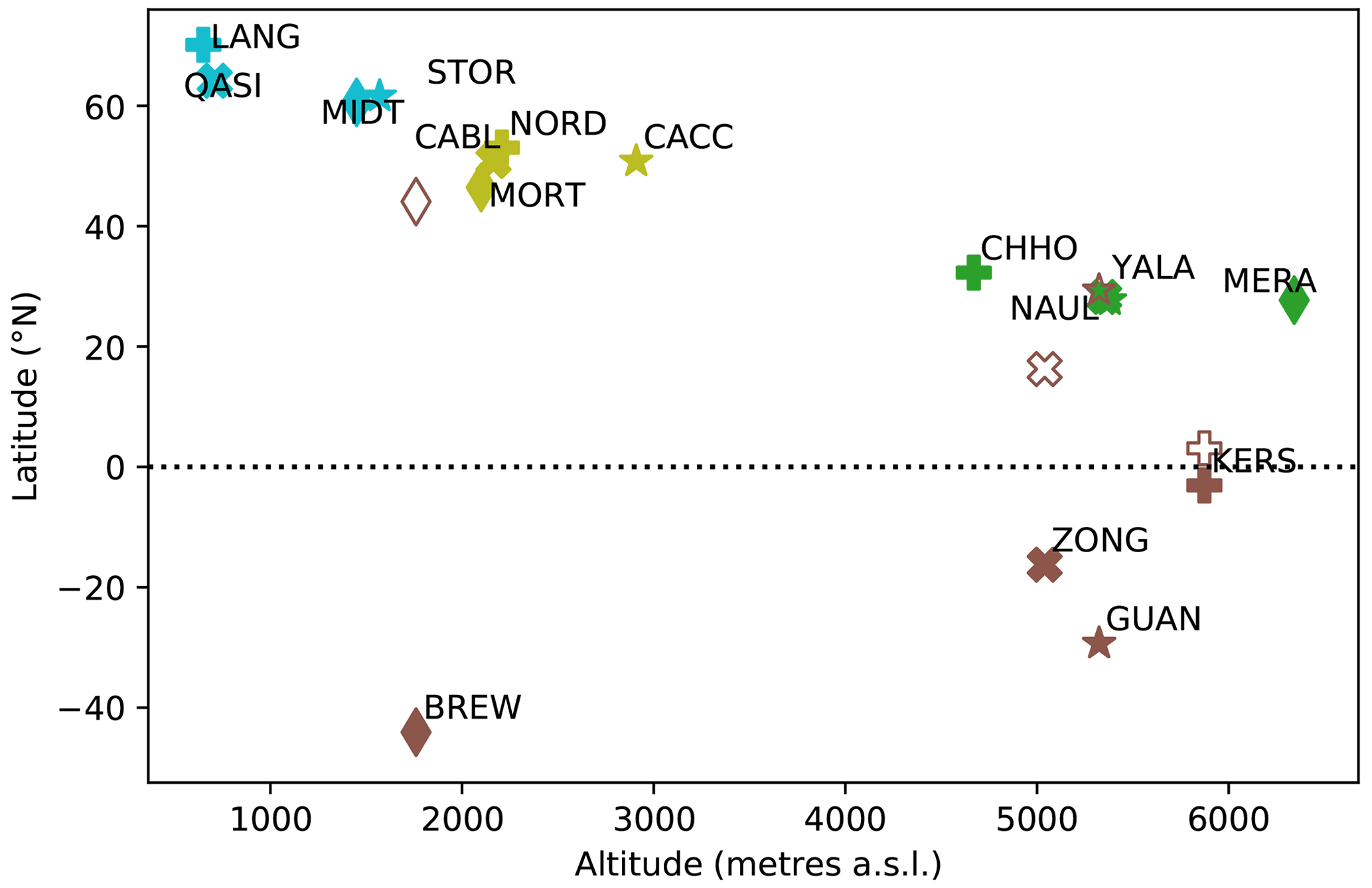
Figure 2Altitude and latitude of study sites. Open symbols show the position of Southern Hemisphere sites against Northern Hemisphere sites for comparison.
As most AWS sites are in ablation areas, they follow a broad pattern of decreasing altitude with distance from the Equator (Fig. 2). Note that two locations have observations in both the ablation and accumulation area – Conrad Glacier (CABL, CACC) and Mera Peak (MERA)–Naulek (NAUL, an ablation area of Mera Glacier). Records from the same site in different years were also joined into continuous records (CABL and NAUL). Records from CABL, CACC and NORD cover only summer periods, and CHHO has three 2-month periods throughout the year; otherwise the records span all months of the year and range from 46 to 3231 d in length (See Table 1 for site name abbreviations). Figures A1 and A2 show monthly average meteorology and SEB fluxes for each site used in the analysis. A few broad groupings of sites (listed in Table 1) can be identified through seasonal trends in near-surface air temperature (Ta; ∘C) or relative humidity (RH) in Fig. A1: mid- and high-latitude maritime and continental sites with strong seasonal cycles of Ta but small variations in RH; Himalayan sites with strong cycles of Ta and distinct wet and dry seasons; tropical sites with small variations in Ta and distinct wet and dry seasons; and a mid-latitude arid site (GUAN) with low RH.
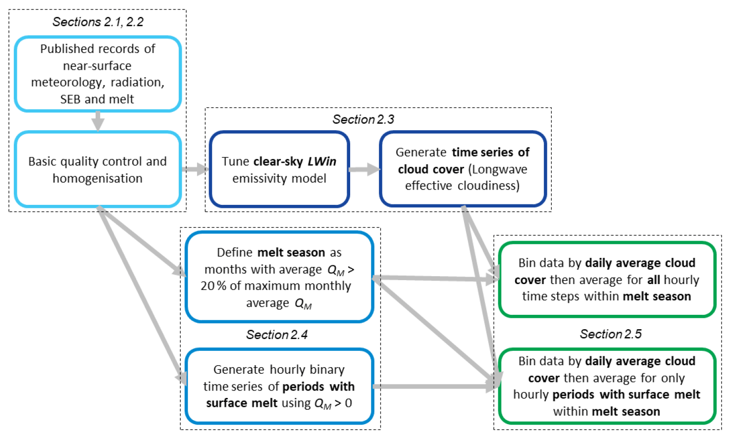
Figure 3Steps used to process and analyse data, annotated with relevant sections of the methods.
2.2 Data processing
Data from each site were taken through several processing steps as outlined in Fig. 3. After basic quality control and homogenisation (described below), a time series of cloudiness was generated for each site (Sect. 2.3) and melting periods and the main melt season were defined (Sect. 2.4), after which cloud effects on melt were analysed (Sect. 2.5).
Basic quality control and homogenisation involved the following steps:
-
sub-hourly data resampled to hourly time steps
-
times converted to local solar time using longitude rounded to nearest full-hour offset from UTC
-
data cut to full days only (no days with partial missing data)
-
naming, units and sign conventions of variables standardised
-
periods with missing radiation data (SWin, SWout, LWin, LWout) removed
-
periods with missing Ta and RH data removed
-
negative values of SWin and SWout set to 0
-
values of LWout >315.6 reset to 315.6 W m−2
-
net radiation (Rnet) calculated from corrected values of (SWin, SWout, LWin, LWout)
-
near-surface vapour pressure (ea; hPa) calculated from Ta and RH using Buck (1981)
-
surface temperature (Ts; ∘C), if not provided, calculated from LWout using the Stefan–Boltzmann law and a surface emissivity of 1
-
daily average albedo calculated as ratio of daily sums of SWin and SWout
-
if QM or surface melt calculated from SEB model is not provided, then QM calculated as positive values of SEB when ∘C, with the slightly relaxed constraint on Ts allowing for some uncertainty in measured Ts.
Monthly statistics (averages, frequencies by bin, etc.) were only calculated when at least 10 d of data from a given month were available.
2.3 Defining clear-sky and cloudy periods using incoming longwave radiation
For each site, time series of cloudiness were derived from measured LWin, ea and near-surface air temperature (Ta,K; K) following Konzelmann et al. (1994) and Conway et al. (2015). First, the effective sky emissivity (εeff) was calculated using
where σ is the Stefan–Boltzmann constant ( W m−2 K−4). While LWin is influenced by emission from surrounding terrain, the sky-view factor at all sites is close to 1, and horizons at all sites are below the limit of the sensor field of view, so no corrections were needed here.
Time series of theoretical clear-sky emissivity (εcs) at each site were defined using the Brutsaert (1975) curve as modified by Konzelmann et al. (1994) with the exponent set to after Dürr Philipona (2006):
where εad is an elevation-dependent dry air emissivity term (varying between 0.18 and 0.23) defined here using εad values determined from radiative transfer modelling in Durr et al. (2006) for the European Alps that are regressed against elevation (z; m above sea level):
For each site, Eq. (4) was fitted to the lowest 10 % of LWin in each of 30 bins (Fig. A3) by finding the value of b (in 0.001 steps) that gave the smallest root mean square error (RMSE). This step used only hours with valid LWin, ea and Ta,K values and RH <80 %. Optimised values of b and RMSE are given in Table A1.
Time series of longwave equivalent cloudiness (Nε) were then derived by fitting hourly measured εeff between theoretical clear-sky (εcs) and overcast (εov=1) emissivity values, limiting Nε to a range from 0 to 1 (Conway et al., 2015):
Following Giesen et al. (2008), clear-sky conditions are defined as Nε≦0.2, partially cloudy as and overcast as Nε≥0.8. Daily average, rather than hourly average, Nε was used to define cloudiness to reduce noise, limit the influence of diurnal cycles in variables and focus on synoptic-scale (daily) variability in cloud–SEB relationships. Note that moderate values of daily average cloudiness can indicate either patchy cloud cover and/or a mix of overcast and clear-sky conditions during a day. Cloudiness can be derived from SWin (e.g. Greuell et al., 1997; Sicart et al., 2006; Mölg et al., 2009a; Kuipers Munneke et al., 2011) but was considered a less appropriate metric here, as its calculation relies on setting a typical cloud extinction coefficient that differs between sites (Pellicciotti et al., 2011). In addition, cloudiness cannot be derived from SWin during the night, and terrain shading of SWin introduces further uncertainty, especially in winter.
2.4 Definition of melt season and periods with surface melt
For each site, a melt season was defined as the months in which monthly average QM at the site was greater than 20 % of the maximum monthly average QM for the same site (Figs. A2, A4). This proved a simple method to retain months with substantial melt but exclude winter months where melt is infrequent. The sensitivity of this choice was assessed by replicating key results using only months with monthly average QM greater than 80 % of the maximum monthly average QM for that site. Rather than only selecting individual melt events for analysis, averages over all time steps in the melt season were used to better understand the relationships between cloudiness, surface radiation and near-surface meteorology, without skewing the data towards melt episodes that may have atypical meteorology. To identify the times surface melt occurred and to quantify the contributions of SEB components to QM, periods with surface melt were defined as hourly time steps with QM>0.
2.5 Analysis of cloud effects
The relationship between cloudiness, meteorology, SEB and melt is assessed by binning the time series of different variables by daily average cloudiness. Five evenly sized bins were used with bin centres at Nε=0.1, 0.3, 0.5, 0.7 and 0.9, with the top and bottom bins corresponding to clear-sky and overcast conditions, respectively. Data within each bin were then averaged across all days within the main melt season to demonstrate the average relationships between cloudiness and different variables.
In Sect. 3.2, 3.3 and 3.4, we use the term cloud effects to describe the change in a variable during cloudy conditions with respect to clear-sky conditions. In studies of net radiation, the cloud effect (CE) is defined as the difference between average and clear-sky conditions (e.g. Ambach, 1974; van den Broeke et al., 2008). Here we extend the concept to QM in order to describe the average change in melt related to clouds, even though clouds are not the only meteorological forcing responsible for changes in QM. We calculate CE for all net radiation components (SWnet, LWnet, Rnet) and QM. Here, we calculate CE by subtracting the average value in the clear-sky bin () from the average value equally weighted across all cloudiness bins. Equally weighting each cloudiness bin ensures that differences in the frequency of different cloud conditions do not skew the data between sites.
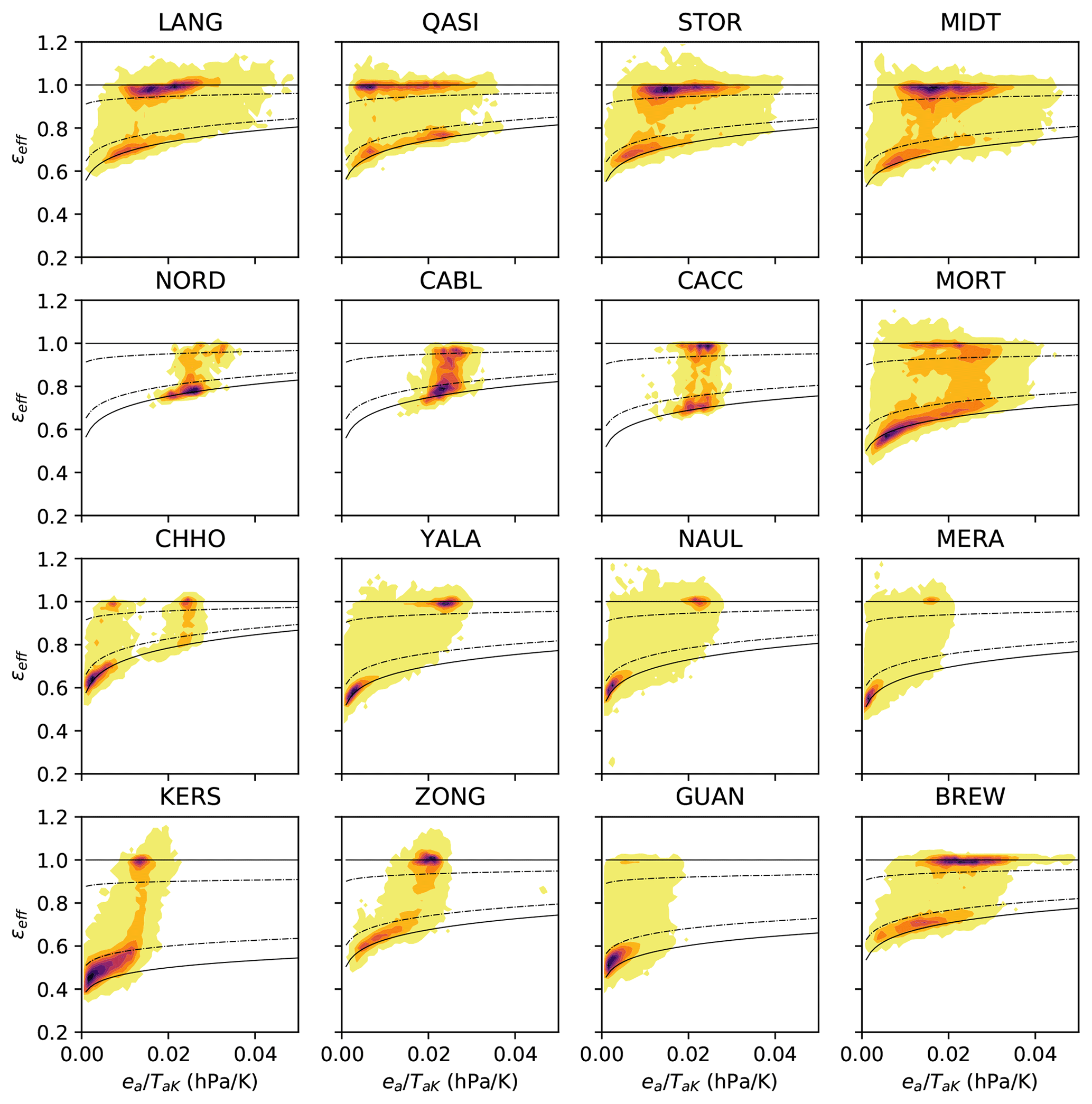
Figure 4Frequency of observed εeff (filled contours) vs. for sites arranged by latitude. Also shown are calculated εcs (lower solid line), εov (upper solid line) and εeff at clear-sky and overcast limits of Nε=0.2 and Nε=0.8, respectively (lower and upper dashed lines, respectively). Contours of relative frequency created from 2D histogram with common x and y bins across all sites with colours in 10 steps between 1 (yellow) and the maximum number of hours in any x, y bin for each site (dark brown–black).
3.1 Cloud metrics
3.1.1 Effective sky emissivity and fitted clear-sky curve
The derivation of clear-sky emissivity from LWin highlighted substantial variations in the relationship between near-surface meteorology and LWin between the sites. On an hourly basis, most sites show a preference for either clear-sky or overcast conditions, as shown by the darker colours around the clear-sky and overcast emissivity (Fig. 4). Sites in the Himalaya (CHHO, YALA, NAUL, MERA) showed a distinct seasonality with predominately warm, wet and overcast or cold, dry and clear-sky conditions. Tropical and arid glacier sites (KERS, GUAN) show a much lower εcs for the same surface vapour pressure, not only due to the high elevation (therefore low εad) but also due to the low value of b (Eq. 4; Table A1), which indicates a thinner atmospheric water vapour profile above the surface compared to Himalayan sites at similar altitudes. Mid-latitude sites with records covering the full annual cycle in Europe (LANG, MIDT, MORT, STOR) and New Zealand (BREW) show a similar preference for cold, dry and clear-sky or warm, wet and overcast conditions, while QASI shows a greater frequency of cloud at lower temperature and vapour pressure. Sites in the Western Cordillera of Canada (NORD, CABL, CACC) and Europe (MIDT, MORT, STOR) show more frequent partially cloudy conditions than many other sites. Note that the short summertime records from Canada (NORD, CABL, CACC) do not capture the full spectrum of conditions at these sites.
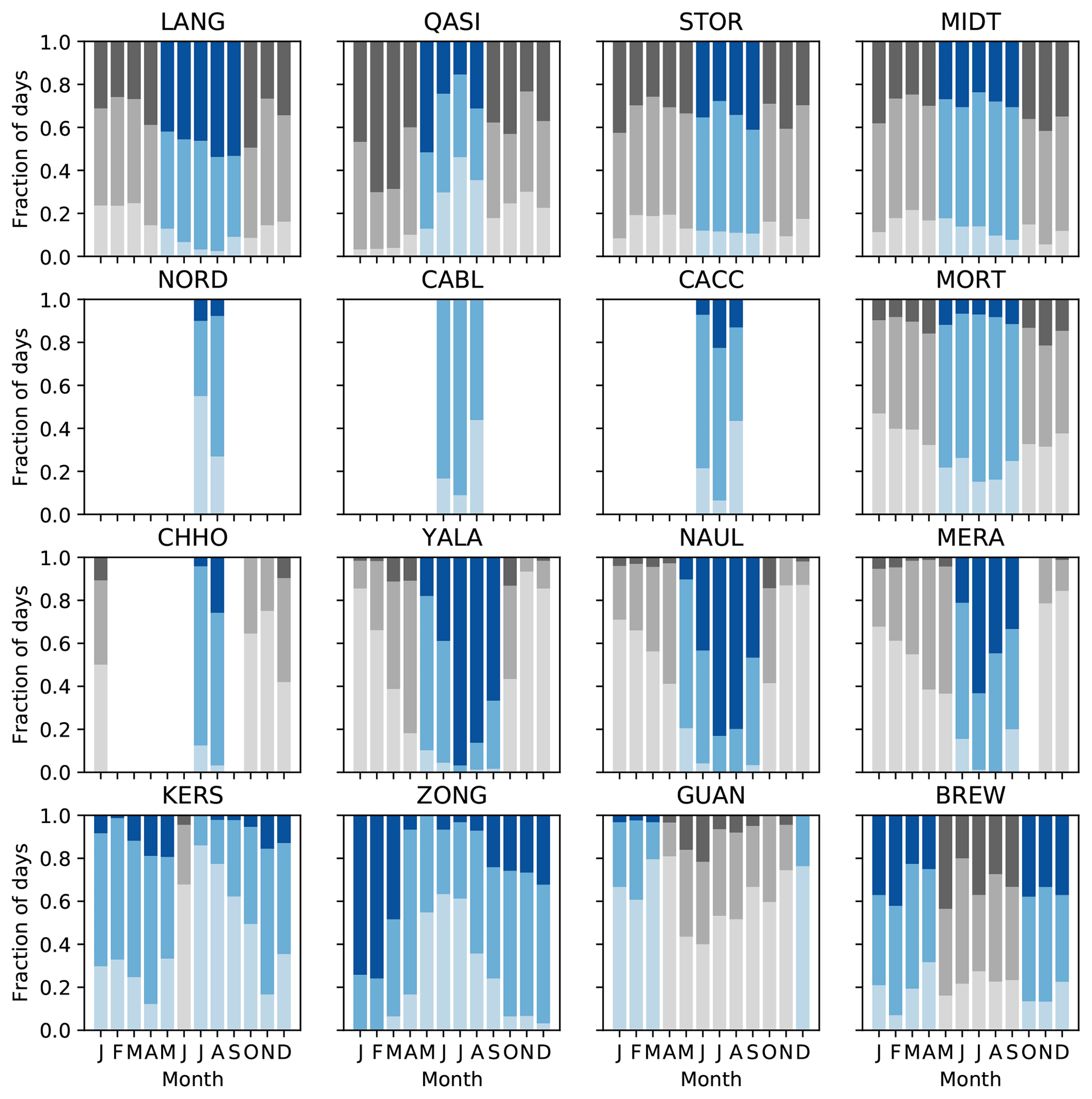
Figure 5Monthly fraction of clear-sky (light shading), partially cloudy (mid shading) and overcast conditions (dark shading) defined using daily average cloudiness (Nε). Months defined as within the melt season are shaded blue.
3.1.2 Monthly cloud frequency
The frequency of clear-sky, partially cloudy and overcast conditions also shows distinct regional and seasonal variations (Fig. 5 for daily average, Fig. A4 for hourly periods). Mid-latitude glaciers in maritime locations show very limited seasonality (BREW, STOR, MIDT) and a high percentage of overcast conditions, except for LANG that displays more frequent overcast conditions during the melt season and QASI that shows a tendency towards more frequent clear-sky conditions during its melt season. Mid-latitude sites in continental locations (NORD, CABL, CACC, MORT) show less frequent overcast and more frequent partially cloudy conditions than the mid-latitude maritime sites, with MORT showing more frequent partially cloudy conditions during the melt season and more frequent clear-sky conditions in the winter. Most Himalayan sites (YALA, MERA, NAUL) show much stronger seasonality, with more frequent overcast conditions during the melt season. The exception is CHHO, which shows weaker monsoon influence (fewer overcast conditions) being on the transition zone between monsoon and arid regions (Azam et al., 2021), though the fraction of partially cloudy conditions still increases in July and August. While ZONG experiences melt most of the year, melt rates are higher during the cloudier months from September through April corresponding with marked seasonal changes in cloud and SEB caused by the tropical climate (Fig. A2). KERS experiences lower cloudiness from June through October, with low melt rates year-round. GUAN experiences the lowest cloudiness, with predominately clear-sky conditions and only sporadic melt during austral summer.
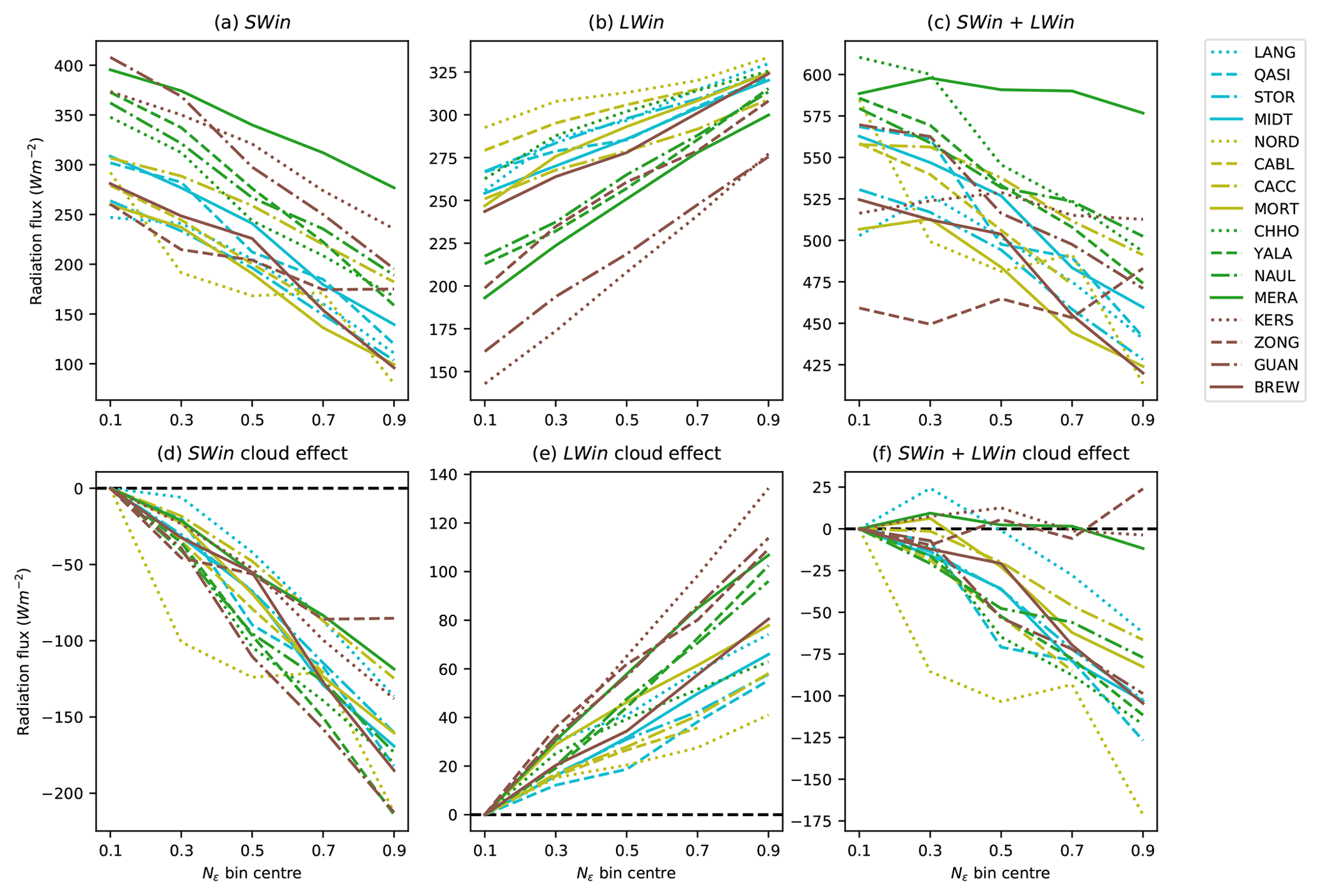
Figure 6(a–c) Average melt-season incoming radiation fluxes (SWin, LWin) for different daily average cloud conditions (Nε). (d–f) As for (a–c) expressed as change from clear-sky conditions (). Note that the y-axis range differs between panels.
3.2 Cloud effects on melt-season surface radiation
An estimate of the direct effect of clouds on the SEB is gained by examining the variation in incoming radiation (SWin and LWin) with cloudiness (Fig. 6). At most sites, the average direct effect of clouds on incoming radiation is negative, steadily decreasing with increasing cloud cover to between −60 and −170 W m−2 (Fig. 6f). The exceptions are the low-latitude and high-altitude sites of KERS, MERA and ZONG, where comparatively small decreases in SWin with cloudiness (Fig. 6d) are compensated by large increases in LWin (Fig. 6e). The large variation in SWin and LWin cloud effects between sites suggests that different cloud types and cloud properties play a role in determining radiative forcing, and this should be investigated in future work. We note that changes in the profile of water vapour and air temperature (estimated by ea and Ta) also influence LWin (and to a much lesser extent SWin). Hence, the direct cloud effects shown here represent the combined effects of direct radiative forcing and changes to atmospheric profiles of water vapour and temperature, in contrast to analyses of cloud radiative forcing that consider the changes in incoming radiation with respect to calculated clear-sky values (e.g. Sicart et al., 2016).

Figure 7(a–c) Average melt-season net radiation fluxes (SWnet, LWnet, Rnet) for different daily average cloud conditions (Nε). (d–f) As for (a–c) expressed as change from clear-sky conditions (Nε≦0.2). Note that the y-axis range differs between panels.
By analysing the change in net radiation fluxes (SWnet, LWnet and Rnet) the effect of albedo and surface temperature is included with the direct effect of clouds on incoming radiation (Fig. 7). A clear increase in Rnet during cloudy periods (positive Rnet cloud effect), a.k.a. radiation paradox, is observed at some sites – ZONG, MERA and LANG (Fig. 7f) – due to the small negative SWnet effect and strong positive LWnet effect (Fig. 7d, e). GUAN and KERS have a similarly strong positive LWnet effect at higher values of Nε, but much more negative SWnet effects cancel these out. For most sites, the Rnet cloud effect is small and negative (0 to −20 W m−2). Many of these sites show a decrease in Rnet only at higher values of Nε, while three sites (MIDT, MORT, CHHO) show the highest Rnet value in partially cloudy conditions, emphasising that the relationship between Rnet and cloudiness is not always linear. NORD, CABL, QASI and CHHO all show a strong negative Rnet cloud effect, driven by a strong negative SWnet effect and weak LWnet cloud effect. For the two sites with measurements from both the accumulation and the ablation areas, accumulation sites exhibit more a positive and/or less negative Rnet cloud effect compared with their ablation area counterparts, driven by the change in the SWnet cloud effect (surface albedo) rather than a large change in the LWnet cloud effect.

Figure 8Average melt-season near-surface meteorology for different daily average cloud conditions (Nε). Dashed lines indicate melting point temperature in (a) and saturation vapour pressure in (c).
3.3 Variation in near-surface meteorology with cloudiness
Alongside radiative changes, differences in near-surface meteorology are also an important driver of SEB and melt variations with cloudiness, particularly QS, QL and LWin. Air temperature shows a divergent relationship to cloudiness; at sites with average melt-season Ta≫0 ∘C, increasing cloudiness is associated with lower temperatures, while at sites with average melt-season Ta<0 ∘C (KERS, MERA, NAUL, YALA), cloudiness is generally associated with higher temperatures (Fig. 8a). Average Ta varies little with cloud cover at ZONG and CHHO. At most sites, wind speed decreases with increasing cloudiness (Fig. 8b). The exceptions are BREW and STOR, which show moderate increases (<1 m s−1); LANG and MIDT, which show larger increases (1.6 and 2.9 m s−1, respectively); QASI, which shows no large change cloudiness; and CACC, which shows peak wind speed at moderate cloudiness. Sites where wind speed increases with cloudiness (particularly MIDT and LANG) have a wind climate that is mainly influenced by the large-scale circulation, while other sites may have a more local wind climate where local or mesoscale katabatic or convective circulations prevail (e.g. Mölg et al., 2020; Conway et al., 2021). Stronger radiative cooling during clear-sky periods may promote higher katabatic wind speeds in clear-sky conditions, though the relationship is not simple; at ZONG, strong winds during clear-sky conditions are related to large-scale forcing during the dry season (Litt et al., 2014). As expected, ea and RH increase with cloudiness; however some sites with ea around the saturation vapour pressure of the melting surface show a weak relationship to cloudiness (e.g. QASI, CACC). The wide variation in RH in clear-sky conditions (∼30 % to ∼70 %) implies that care should be taken when using RH to model cloud cover using empirical parameterisations developed for particular study areas or even at different altitudes (e.g. NAUL vs. MERA).
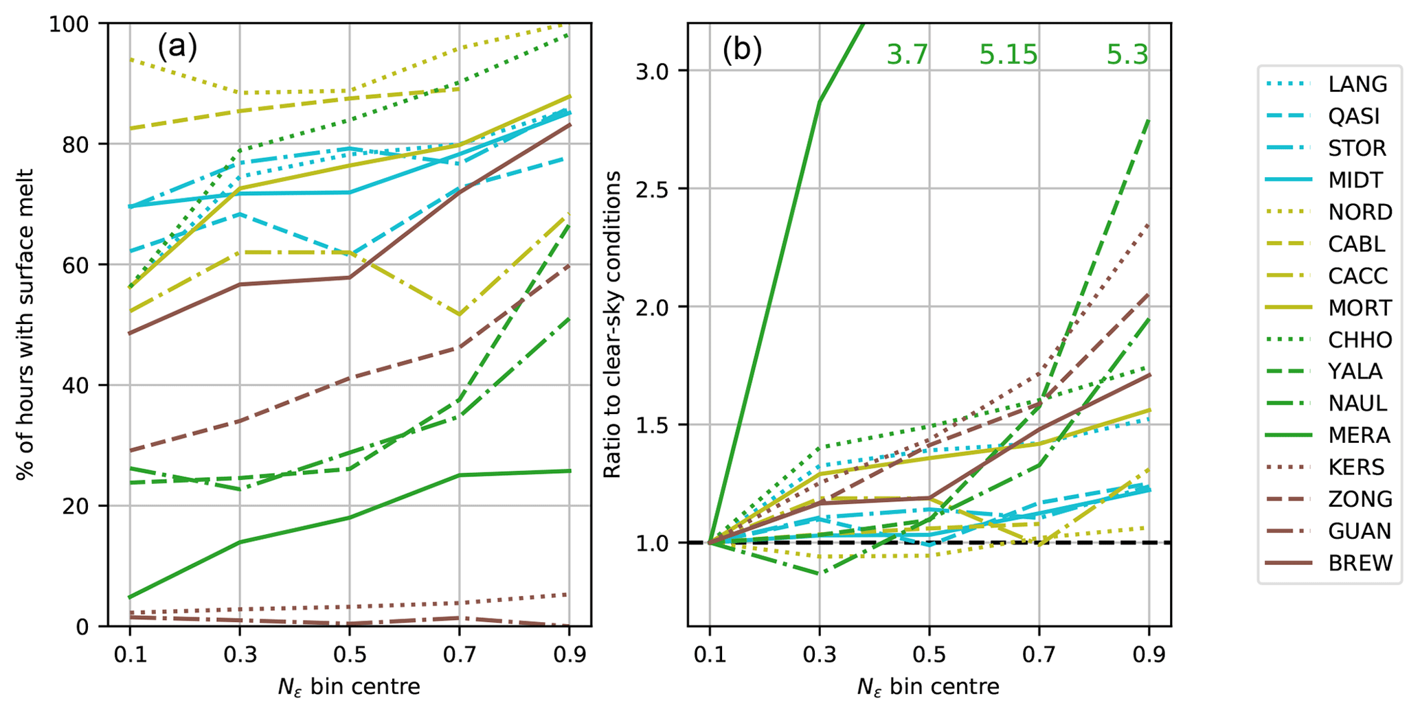
Figure 9(a) Percentage of hours with surface melt for different cloud conditions (Nε) during the melt season. (b) As for (a) shown as a fraction with respect to clear-sky conditions (Nε≦0.2). Note that GUAN is excluded from (b) due to insufficient data points and that for clarity some points for MERA are shown as text within the panel.
3.4 Variation in melt frequency, melt amount and SEB with cloudiness
The percentage of hours with surface melt increases with cloudiness at all study sites (Fig. 9), except for GUAN, which experiences very infrequent melt in all conditions. Colder sites across the Himalaya and tropical regions (except KERS) show the largest increases with respect to clear-sky conditions (up to 5 times more frequent), while BREW, MORT and LANG all show moderate increases up to 1.5 times more frequent in overcast conditions. Other European and North American sites show comparatively high melt frequency across all cloud conditions, indicative of the warm conditions where ea exceeds that of a melting ice–snow surface. Even in these conditions, periods with surface melt still become more common with increasing cloudiness, with 100 % of overcast periods at NORD experiencing melt (Fig. 9a). While analysis of diurnal patterns of melt is beyond the scope of this paper, the higher percentage of hours with melt during overcast conditions indicates that nighttime melt is more frequent during overcast periods. MERA shows the largest increase in melt frequency with cloudiness, with melt 5 times more frequent in overcast (26 % of overcast conditions) compared to clear-sky conditions (5 %). A consistent increase with cloudiness is observed at MERA, but caution is warranted given the small number of hours with melt in clear-sky conditions (20 h).
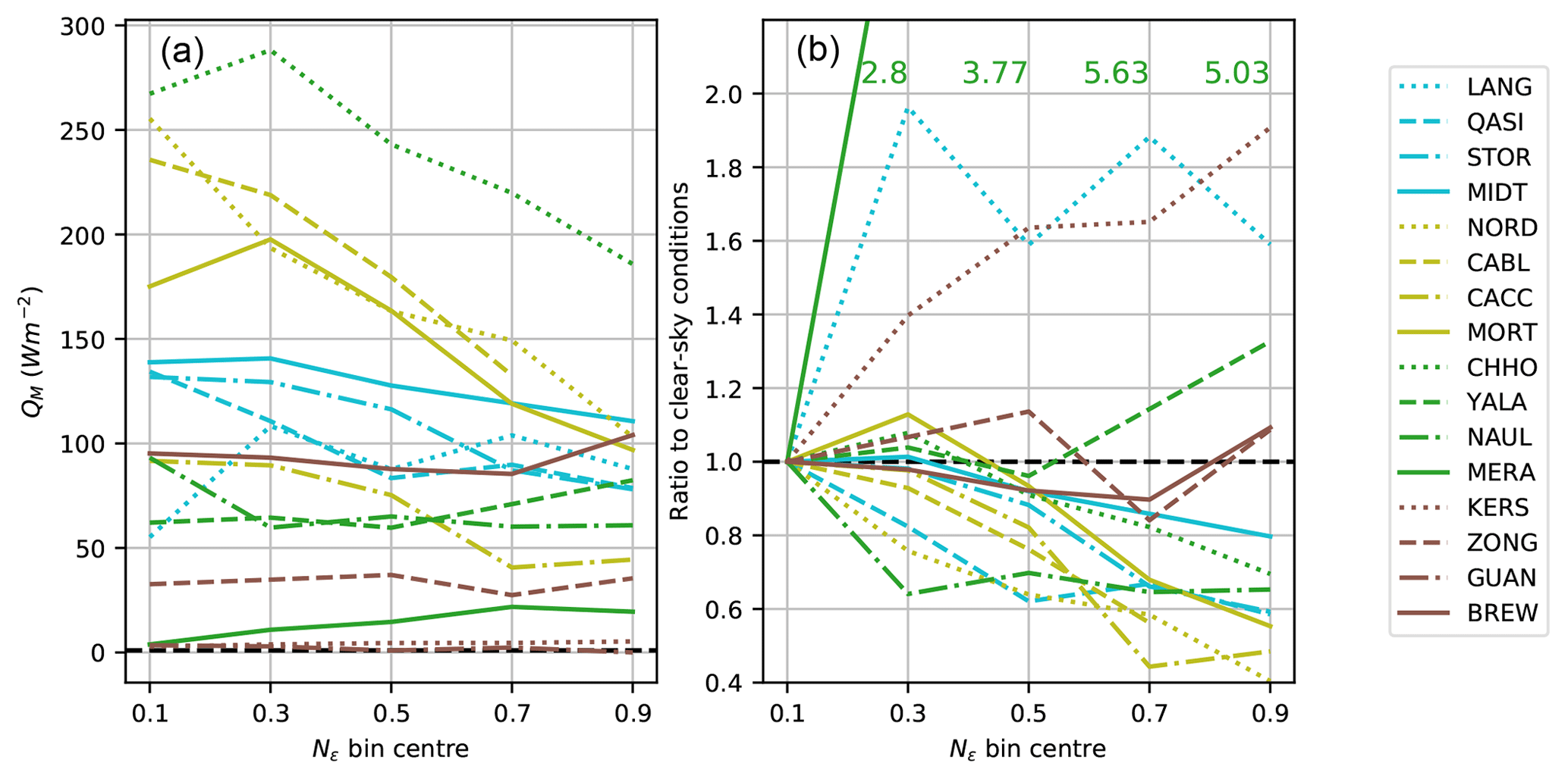
Figure 10(a) Average melt-season QM for different cloud conditions (Nε). (b) As for (a) shown as a fraction with respect to clear-sky conditions (Nε≦0.2). Note that GUAN is excluded from (b) due to insufficient data points and that for clarity some points for MERA are shown as text within the panel.
In contrast to the percentage of hours with surface melt, the relationship between the amount of energy available for melt (QM) and cloudiness does not show a universal variation, with sites showing increased, decreased or no change with increasing cloudiness on average (Fig. 10). Around half the sites show a general reduction in daily average QM with increasing cloudiness, particularly those in North America (CABL, CACC, NORD) and some European sites (MIDT, MORT, STOR) along with QASI and CHHO. LANG, MERA and KERS show large relative increase in QM with cloudiness, while BREW, ZONG and YALA show a more mixed response with a small increase in melt in overcast conditions. LANG and NAUL display a sharp change from clear-sky conditions to the first partially cloudy bin (Nε∼0.3) but little change with increasing cloudiness.
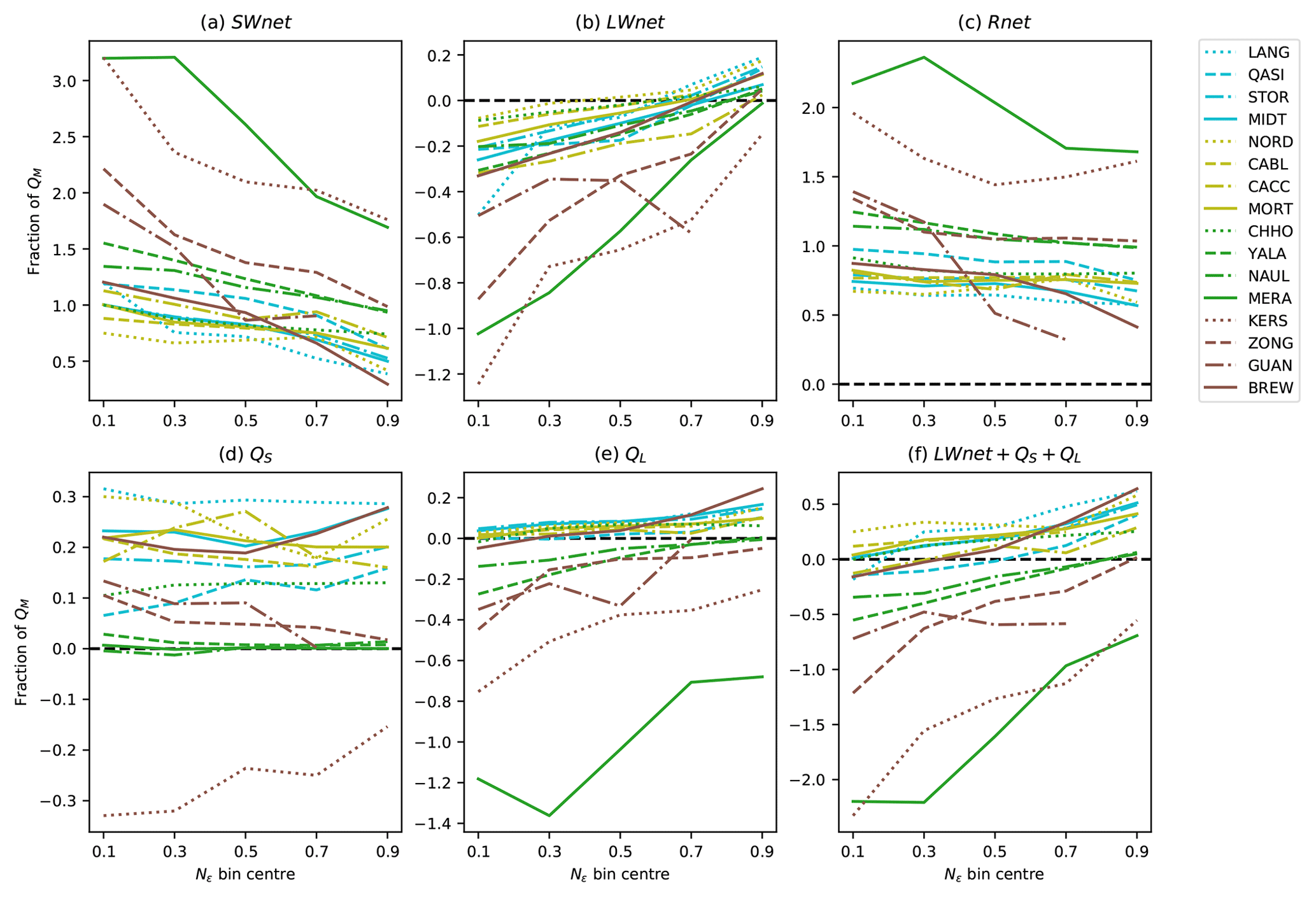
Figure 11Average melt-season SEB terms during hours with surface melt for different cloud conditions (Nε). Variables are shown as a fraction of average QM during hours with surface melt in each respective cloud condition (Nε). Note that the y-axis range differs between panels.
As cloudiness increases, the source of QM changes; at all sites, the contribution of SWnet reduces and a greater proportion of QM comes from the temperature-dependent fluxes (LWnet, QS and QL) (Fig. 11a, f; see Fig. A5 for absolute values). At almost all sites, LWnet changes sign with cloudiness, from an energy sink in clear-sky conditions to an energy source in overcast conditions. At colder and drier sites (KERS, MERA, GUAN, NAUL, YALA, ZONG), negative QL reduces QM during clear-sky periods, but this effect reduces towards 0 as cloudiness increases. At the coldest sites (KERS, MERA and ZONG), QL remains negative during melt (indicating evaporation as Ts=0 ∘C) even in overcast conditions. At BREW and CHHO, QL switches sign with cloudiness, from an energy sink during clear-sky conditions to an energy source in overcast conditions, while other mid- and high-latitude sites show modest increases in QL with cloudiness. Small QS fluxes at MERA, NAUL, YALA and ZONG are due to Ta values during melt remaining around 0 ∘C. At other sites, the proportion of melt from QS remains fairly static with cloudiness, despite decreasing in absolute magnitude (Fig. A5) due to decreases in Ta (Fig. 8a). The exceptions are BREW, MIDT and QASI, where the contribution from QS increases with cloudiness, and ZONG, where the contribution of QS decreases. Note that as Fig. 11 presents averages for only periods with surface melt, LWout is constant and that changes in LWnet are entirely due to LWin.
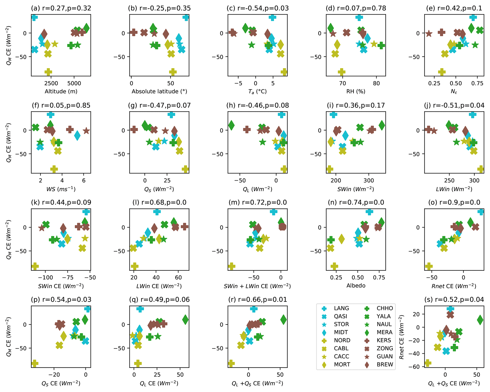
Figure 12The variation in average melt-season QM cloud effect (CE) with (a) station altitude; (b) absolute station latitude; and average melt-season (c) Ta, (d) RH, (e) Nε, (f) wind speed (WS), (g) QS, (h) QL, (i) SWin, (j) LWin, (k) SWin CE, (l) LWin CE, (m) SWin+LWin CE, (n) albedo, (o) Rnet CE, (p) QS CE, (q) QL CE and (r) Qs+QL CE. (s) Variation in Rnet CE with Qs+QL CE. See Sect. 2.5 for definition of CE. Average melt-season values are calculated by averaging values from the five cloudiness bins equally.
3.5 Relationships between QM cloud effect and site characteristics
While the average change in QM with cloudiness is small at some sites, it is instructive to assess whether the melt-season average QM cloud effect (CE) at the various sites can be related to geographic or climatic parameters. Figure 12a and b show that the relationship between average cloudiness and melt at the various sites does not directly relate to latitude or altitude. Average near-surface air temperature is moderately correlated to QM CE (Fig. 12c). Sites with lower Ta (e.g. MERA, KERS) generally have smaller QM CE than sites with higher high Ta (NORD, CABL, MORT) but with some notable exceptions (e.g. LANG has positive QM CE with relatively high Ta). Average cloudiness shows some association with QM CE, with clearer sites tending to have more negative QM CE (Fig. 12e), with the exception of tropical/arid sites with predominately clear skies (KERS, GUAN) that show neutral QM CE. Neither average wind speed nor relative humidity shows a clear relationship with the QM CE (Fig. 12d, f). Average turbulent heat fluxes and LWin are moderately correlated with QM CE (Fig. 12g, h, j), largely following the pattern of sites shown for Ta, while average SWin is not significantly correlated (Fig. 12i).
Considering the association of radiative and melt cloud effects, average incoming radiation cloud effects explain some of the variance of QM CE, with LWin (Fig. 12l) showing a stronger association than SWin CE (Fig. 12k). Combined, the incoming radiation cloud effects can explain over half (53 %) of the variation in QM CE (Fig. 12m). Surface albedo has a similar correlation to QM CE (Fig. 12n) as the incoming radiation cloud effects together. The combination of these into the Rnet CE shows the clearest relationship to QM CE (Fig. 12o). In general, sites that experience a radiation paradox (LANG, ZONG, MERA) also experience greater melt in cloudy conditions (positive QM CE), while sites with negative Rnet CE experience less melt in cloudy conditions (Fig. 12o).
Turbulent flux cloud effects are also moderately correlated to melt-season average QM CE (Fig. 12p, q) and when combined explain approximately 44 % of the variance in QM CE (Fig. 12r). Thus, sites where QS decreases with cloudiness show more negative QM CE. Sites where QS varies little with cloudiness and/or QL becomes less negative/more positive during cloudy periods show neutral or positive QM CE. Interestingly, the radiative and turbulent heat cloud effects show a moderate association, with sites with large negative Rnet CE also having a negative net turbulent flux cloud effect and vice versa (Fig. 12s).

Figure 13As for Fig. 10 but only for months with >80 % of maximum monthly average QM. Note GUAN and KERS are excluded from (b) due to insufficient data points.
4.1 Regional and elevational patterns
Two groups of sites with a broadly similar response emerge from the above analyses, largely split by latitude, as well as air temperature and continentality. The first group (YALA, NAUL, MERA, KERS, ZONG) consists of high-altitude sites in tropical regions and the Himalaya (excluding CHHO). These sites are comparatively cold, with negative QL and low QS during melt (Fig. A5d, e). During cloudy conditions, these sites experience warmer and calmer conditions (Fig. 8a, b), reduced evaporation/sublimation (less negative or, at times, positive QL; Fig. A5e), and a large increase in the fraction of time that melt occurs (Fig. 9), regardless of the seasonality of clouds or the typical cloud conditions (e.g. KERS vs. MERA). These sites also generally experience greater QM in cloudy periods (except for NAUL; Fig. 10) when averaged over a long melt season that includes months with marginal melt conditions. Some sites experience a radiation paradox where Rnet increases with cloudiness, while others show a small decrease in Rnet with cloudiness (Fig. 7f). While GUAN experiences similar patterns of near-surface meteorology and radiation as the sites in this group, it experiences very infrequent melt (Fig. 9a).
The second group consists of the mid- and high-latitude sites outside the Himalaya (LANG, QASI, STOR, MIDT, NORD, CABL, CACC, MORT, BREW) as well as CHHO. These sites experience higher average melt-season Ta, and Ta generally decreases with cloudiness (Fig. 8a). Despite decreased Ta, melt becomes more frequent in cloudy conditions (Fig. 9). With a few exceptions (e.g. BREW, LANG), QM decreases with increased cloudiness, though the magnitude of decrease varies widely (from 20 % to 60 % less in overcast compared to clear-sky conditions; Fig. 10). CHHO stands out from the other Himalayan sites in that it has higher average Ta that does not vary greatly with cloudiness (Fig. 8a). Here also, low albedo drives a strong negative Rnet cloud effect (Fig. 7f) that, in turn, drives a large decrease in QM during cloudy periods (Fig. 10). At all these sites, QS is positive in all cloud conditions (Fig. 11d), though the absolute magnitude is generally reduced in cloudy periods due to decreased Ta (Fig. A5d). Clouds are associated with increased wind speed at most maritime sites (LANG, MIDT, STOR, BREW; Fig. 8b) but do not show a consistent relationship to QM (Fig. 10); MIDT and STOR experience less QM in cloud conditions, whereas LANG and BREW experience greater QM due to increased wind speed and comparatively modest decreases in Ta that drive increased LWnet and more positive QL (Fig. A5e). In the case of LANG, increased QM during cloudy conditions is also due to a positive Rnet cloud effect (Fig. 7f).
Locations with AWS at two elevations highlight more positive Rnet cloud effects at accumulation sites than ablation sites due to the higher albedo (Fig. A1) and larger difference between clear-sky and overcast emissivity (Fig. 4). Differences in melt are stronger at the Himalayan pair (NAUL, MERA), where melt is decreased in cloudy conditions at the lower sites and increased in cloudy conditions at the upper site (Fig. 10). At the pair in Canada (CABL, CACC), both sites experience reduced melt during cloudy conditions, though in absolute terms, the decrease is larger in the ablation area.
4.2 Limitations
The derivation of cloudiness from LWin also poses challenges. At some sites (e.g. LANG and MORT), εcs shows a poor fit at higher vapour pressure, with incoming LWin during clear-sky periods being higher than that expected from the theoretical curves (Fig. 4). This mismatch between theoretical and observed εcs during periods of higher ea may cause some clear-sky periods to be misclassified as being in the first partially cloudy bin (3). Indeed, at both LANG and MORT, the Nε∼0.3 bin shows higher melt, indicating this may be the case. The reasons for this mismatch have not been investigated, but it may be due to a different method used to correct LWin data (Giesen et al., 2014) or changes in water vapour profiles in the atmospheric boundary layer. There is also some unavoidable degree of circularity in analysing longwave radiation fluxes (Figs. 6 and 7) that have also been used to derive cloudiness. However, as LWin depends not only on cloudiness but also on variations in Ta and RH, the circularity is not complete. For instance, at Brewster Glacier, the increase in LWin between clear-sky and overcast conditions is approximately the same as the change in clear-sky LWin due to seasonal variations in Ta. Because the method used to calculate cloudiness accounts for the effect of Ta and RH on LWin, the effect of these variations in near-surface meteorology on LWin is retained in the analyses shown in Figs. 6 and 7.
While efforts have been made to homogenise the datasets, it is possible that biases still affect the results. Interannual variability causes uncertainty, particularly for sites with only one or two seasons (e.g. NORD, ZONG). Giesen et al. (2008; Table 4) show that at MIDT, the contribution of SEB components to melt during clear-sky periods can vary up to 12 % between years, while variability in overcast periods is less. The interannual variability is partly influenced by the seasonality of anomalies in cloudiness, with strong anomalies in spring causing the contribution of QS to melt to change markedly. Some sites also have discontinuous records (CABL, CACC, NORD, CHHO) that do not include periods with lower melt rates outside the peak melt season. Increased clear-sky solar radiation and Ta as well as decreased albedo during the peak melt season are likely to cause Rnet and QM cloud effects to be larger at these sites compared to those with longer records that include periods of more marginal melt. This effect is demonstrated by repeating the analysis but restricting the melt season to months with at least 80 % of the maximum monthly average QM: 2–3 months at each site (Fig. A6). Figure 13 shows the relationship between average QM and Nε for the period with peak melt rates at each site. The previously large increase in QM with clouds at MERA and LANG becomes more variable, and QM is smaller in overcast compared to clear-sky conditions. This is primarily due to the removal of months with a high-albedo snow surface in the early season, where a strong radiation paradox drives an increase in melt during cloud periods. In clear-sky conditions, higher Ta and ea in the peak melt season creates generally positive QL at these sites (not shown). BREW also now shows a moderate decrease in QM with clouds, while ZONG shows a much stronger decrease due to marked seasonal changes in the SEB terms driving melt (less negative LWnet and QL in austral spring and summer; Fig. A2). Only one site (YALA) still shows its highest QM in overcast conditions, but the increase is small compared to the average for the longer melt season. In fact, at outer-tropical sites such as ZONG where melt can occur in most months alongside large seasonal variations in precipitation and cloudiness, the analysis here likely mixes cloud effects with seasonal changes in other meteorological forcings (such as potential solar irradiance, humidity and air temperature).
Seasonal changes in cloud effects on melt have been previously reported by some studies; Giesen et al. (2008) show that negative QM cloud effects at MIDT were restricted to July and August, with other months showing neutral or positive cloud effects; Conway and Cullen (2016) show only one month with negative QM cloud effect at BREW, with positive effects in other months; Chen et al. (2021) report strong negative QM cloud effects in July and August for Laohugou Glacier No. 12 in the western Qilian Mountains of China, with weaker negative effects in May and June and neutral effects in September. To elucidate spatial patterns of net melt cloud effect, future studies should investigate seasonal patterns of cloud effects and establish the timing of transitions between periods of positive and negative QM CE and how these relate to Rnet CE and surface meteorology. It is likely that the timing of transition from positive to negative QM CE will therefore determine the melt-season average cloud effects. To this end, there is a need to capture AWS records through the full annual cycle at study sites in order to fully understand the relationships between meteorological forcing and melt.
4.3 Mechanisms influencing SEB changes with clouds
In addition to the key role that surface albedo plays in determining Rnet, there are three key mechanisms that drive temporal changes in SEB with cloudiness:
- i.
direct forcing of incoming radiation (decreased SWin and increased LWin)
- ii.
changes to near-surface meteorology that alter turbulent heat fluxes
- iii.
surface and subsurface temperature feedbacks that alter net radiative and turbulent fluxes.
Here we demonstrate that direct forcing of incoming radiation and surface albedo explains much of the net effect of clouds on QM across sites. The high correlation between melt-season average Rnet CE and QM CE between sites (Fig. 12), along with the sensitivity of these averages to the length of the melt season (Fig. 10 vs. Fig. 12), underlines the primary control of direct and indirect radiative mechanisms on determining the sign of melt response to clouds. It is likely that substantial seasonal variations in Rnet CE exert the primary control on the effect of clouds on glacier melt.
Changes in turbulent heat flues with cloudiness tend to be smaller in magnitude than changes in Rnet (Fig. A5), except for the more extreme cases where air temperature changes greatly with cloudiness, e.g. NORD, where QS markedly decreases with cloudiness, and MERA, where QL becomes far less negative in cloudy conditions. Despite this, net turbulent heat flux cloud effects show moderate correlation to QM CE, and thus changes in near-surface meteorology play a significant role in determining the net response of melt to clouds. These findings echo those of Liu et al. (2021), who show increased melting during cloudy periods on Mt Everest are due to increased Rnet as well as lower wind speeds that drive smaller losses to QL, and Conway et al. (2016), who found changes to QL contributed to increased melt during cloudy periods. Future work should assess the mechanisms driving the observed covariance between cloudiness and near-surface meteorology at different sites. For example, do large-scale changes in air mass or local/mesoscale processes drive changes in Ta in different cloud conditions? How well are these processes represented in the datasets used to force glacier melt models on regional scales? Seasonal changes in the relative magnitudes of turbulent and radiative cloud effects also deserve further scrutiny.
Surface temperature responds quickly to changes in SEB, and here we show that during cloudy periods, a melting state is observed more frequently, in line with previous research on maritime glaciers (Conway et al., 2016). We have not attempted to further analyse surface and subsurface temperature feedbacks here, as not all datasets contain these variables. A detailed analysis is more suited to sensitivity experiments that allow for the transient response of subsurface temperature, humidity and refreezing to be resolved.
The increased frequency of melt during cloudy conditions, especially at higher elevations, raises the question of how glacier-wide melt is altered by clouds, along with how glacier-wide surface mass balance is altered by refreezing. Van Tricht et al. (2016) show increased runoff from the Greenland Ice Sheet during cloudy periods due to increased melt extent and decreased refreezing of meltwater, while Niwano et al. (2019) found clouds increase melt extent but reduce total melt due to feedbacks between cloudiness and near-surface humidity. These studies are in line with the findings here – that clouds enhance the possibility of melt at a given site, by removing large negative LWnet and QL fluxes to precondition the surface to melt, but do not necessarily cause greater melt unless albedo is high enough to cause a radiation paradox or unless increased near-surface air temperature, humidity and/or wind speed causes an increase in net turbulent fluxes.
4.4 Implications for glacier melt modelling
Previous research that identified a higher sensitivity to warming associated with clouds at BREW (Conway and Cullen, 2016) showed this occurred without increased melt during cloudy periods. The effect was primarily due to increased melt frequency and temperature-dependent fluxes during cloudy periods as well as accumulation–albedo feedbacks. All sites analysed here show increased melt frequency and temperature-dependent fluxes during cloudy periods, suggesting more sites may also experience a higher sensitivity to warming associated with clouds. While a formal analysis is beyond the scope of this paper, we may therefore expect that the response of melt to past and future temperature change will be modified by changes to atmospheric moisture in the form of clouds and vapour fluxes. The simplified temperature index models that are generally used to predict future glacier change on global and regional levels (e.g. Marzeion et al., 2018; Huss and Hock, 2018; Zekollari et al., 2019) do not account for these effects. Enhanced temperature index models that can account for changes in cloudiness through solar radiation (e.g. Pellicciotti et al., 2005) only include the opposite effect – a reduction in solar radiation by clouds – and therefore may underestimate future melt at sites where cloud cover is not universally associated with reduced melt (e.g. high-altitude and maritime glacier sites). Given the positive effect of clouds on net radiation at snow-covered and high-altitude sites, future increases in cloud cover may promote further melt, especially during marginal melt seasons and especially at high elevations. However, caution is warranted in making generalisations, as the analysis here shows that even in this set of 16 glaciers, we find variability in the links between clouds and melt, and it seems that some processes are site specific even in this small sample.
The non-linear relationships between clouds and melt motivates the use of SEB models in regional and global assessments of glacier response to climate change. To aid in the development of globally and regionally applicable SEB models and parameter sets, the research community should investigate creating a central open-source repository for glacier AWS and SEB datasets along with supporting metadata. Such a repository would facilitate the easy transfer of data between researchers, streamline processing by establishing data format and metadata standards, and motivate the use of best practices in data collection and quality control. Alongside this, careful assessments of SWin and LWin and their relationship to near-surface meteorology from global, regional and mesoscale meteorological models should be undertaken to ensure uncertainties in model input data are reduced and to assess the need for downscaling to account for local-scale processes. As many glacier SEB models rely on empirical relationships between SWin and LWin to modify these variables to account for local-scale changes in near-surface meteorology (e.g. Mölg et al., 2009a; Conway et al., 2015), globally applicable parameterisations of SWin and LWin should be tested.
A total of 16 high-quality published datasets of near-surface meteorology, radiation and surface energy balance over glaciers in very different climate settings have been homogenised and analysed in a common framework. The analyses sought to assess how the relationships between clouds, near-surface meteorology and surface energy balance vary in different mountain glacier environments. Distinct regional differences in the seasonality of cloudiness are demonstrated between different mountain glacier environments.
On average, over the main period of melt at each site the following is demonstrated:
-
Near-surface humidity (both relative and absolute) is shown to universally increase in cloudy conditions. In contrast, a divergent relationship is found between near-surface air temperature and cloudiness; at colder sites (average near-surface air temperature in melt season <0 ∘C), air temperature is increased in cloudy conditions, while for warmer sites (average near-surface air temperature in melt season ≫0 ∘C), air temperature decreases in cloudy conditions. In essence, air temperature tends towards the melting point of ice in cloudy conditions. Wind speed shows a mixed association to cloudiness at different sites.
-
Most sites, on average, show a modest to strong decrease in net radiation during cloudy conditions during the melt season. A few sites show a clear increase in net radiation with clouds – a.k.a. radiation paradox – but this result is sensitive to the months used in the analysis due to seasonal changes in incoming radiation fluxes and albedo.
-
At all sites, surface melt is more frequent in cloudy compared to clear-sky conditions.
-
At all sites, temperature-dependent fluxes contribute a larger fraction of melt energy during cloudy conditions, primarily due to increased incoming longwave radiation and less negative and/or more positive turbulent latent heat fluxes. The contribution of turbulent sensible heat generally varies little with cloudiness.
-
Cloud cover does not affect daily total melt in a universal way; some sites show average melt energy increases in cloudy conditions, while at other sites, average melt energy decreases. The complex association of clouds and melt energy is due to the interaction of multiple physical processes (direct radiative forcing, surface albedo, co-variance with temperature, humidity and wind) that force it to vary widely with the latitude, average melt-season air temperature, degree of continentality, season and elevation. Overall, the association of clouds and melt is most closely related to net radiation cloud effect, with sites displaying a radiation paradox also showing an increase in energy for melt in cloudy conditions.
-
It is likely that substantial seasonal variations in Rnet CE exert the primary control on the effect of clouds on glacier melt, through changes in surface albedo and the balance of incoming radiation fluxes. Changes in net turbulent fluxes also play a role, and the mechanisms driving co-variance between clouds and near-surface air temperature, humidity and wind speed should be more widely explored.
The non-linear relationships between clouds, near-surface meteorology and melt motivate the use of physics-based surface energy balance models for understanding future glacier response to climate change, particularly in areas where atmospheric moisture plays a key role both in accumulation and ablation processes (e.g. Himalaya, tropical glaciers, maritime glaciers). Future work should also look to carefully assess shortwave and longwave radiation fluxes and their relationships with near-surface meteorology in global, regional and mesoscale meteorological model analyses if we are to confidently use these tools to better understand how future glacier melt will respond to changes in atmospheric temperature.
Table A1Optimised clear-sky emissivity coefficients and error in εcs.
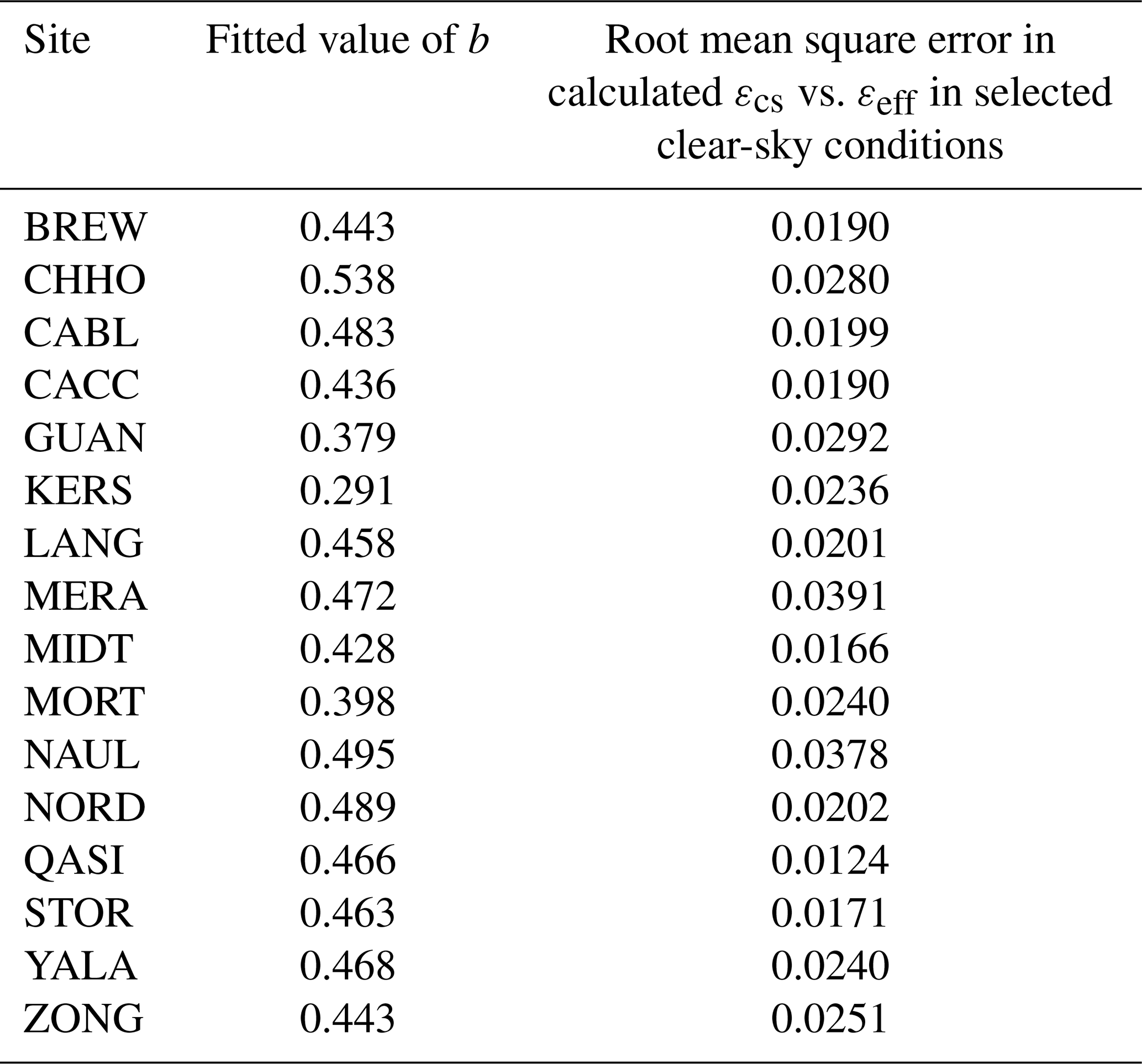
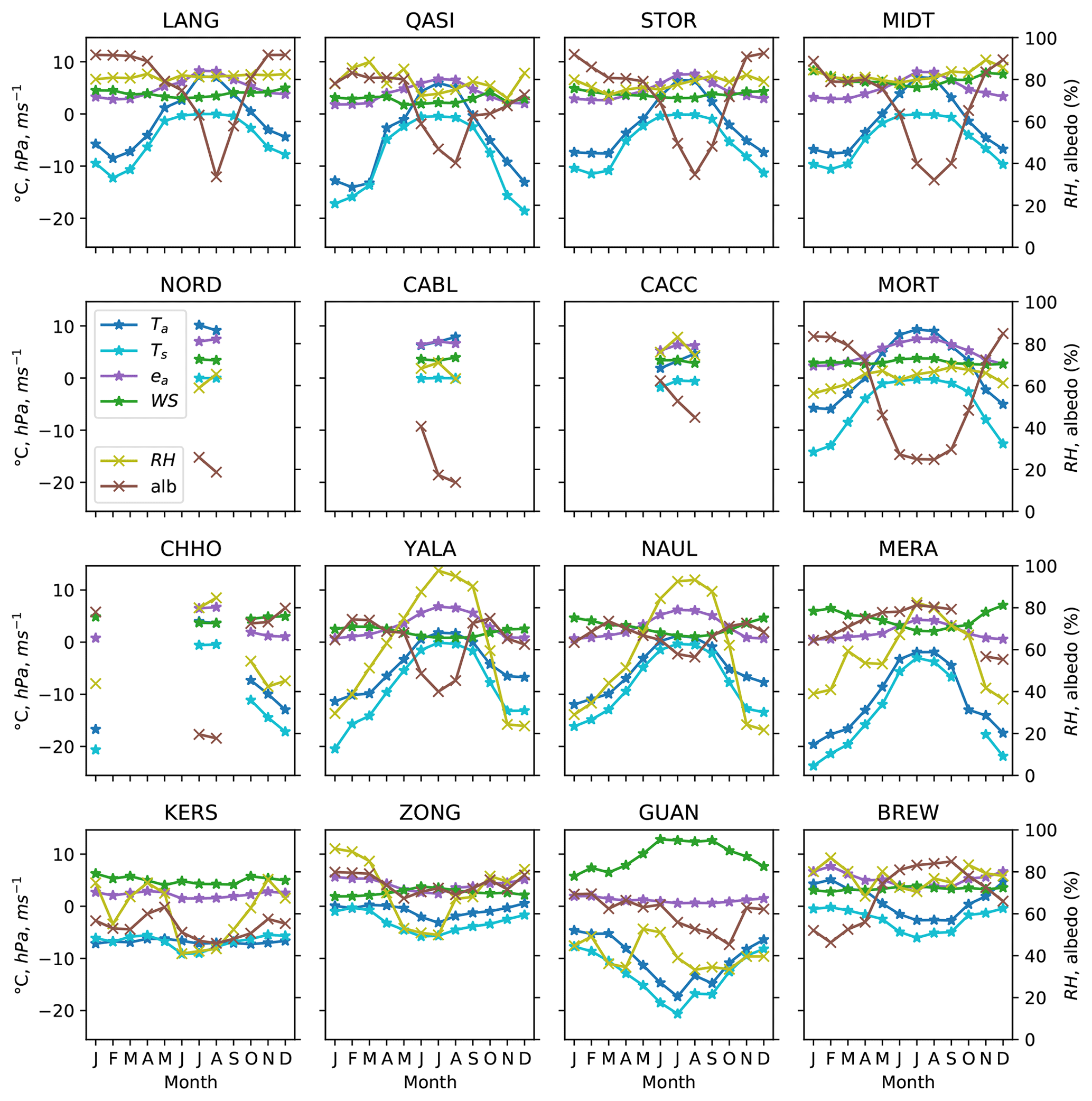
Figure A1Monthly average near-surface meteorological conditions at each site. Note that the monthly value is only shown for a site if it has >10 complete days in a month across the full record.
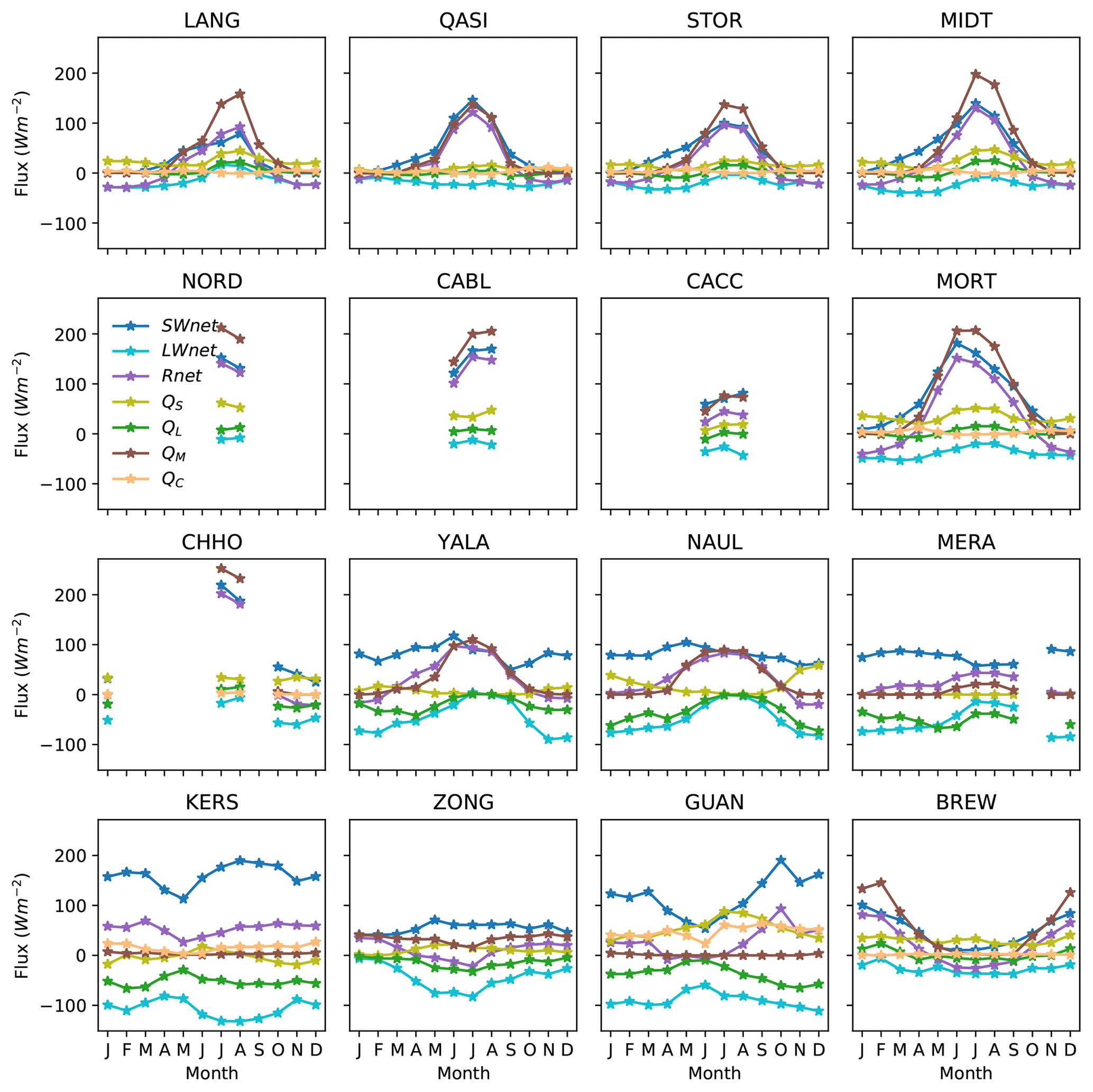
Figure A2Monthly average SEB fluxes at each site. Note that the monthly value is only shown for a site if it has >10 complete days in a month across the full record.
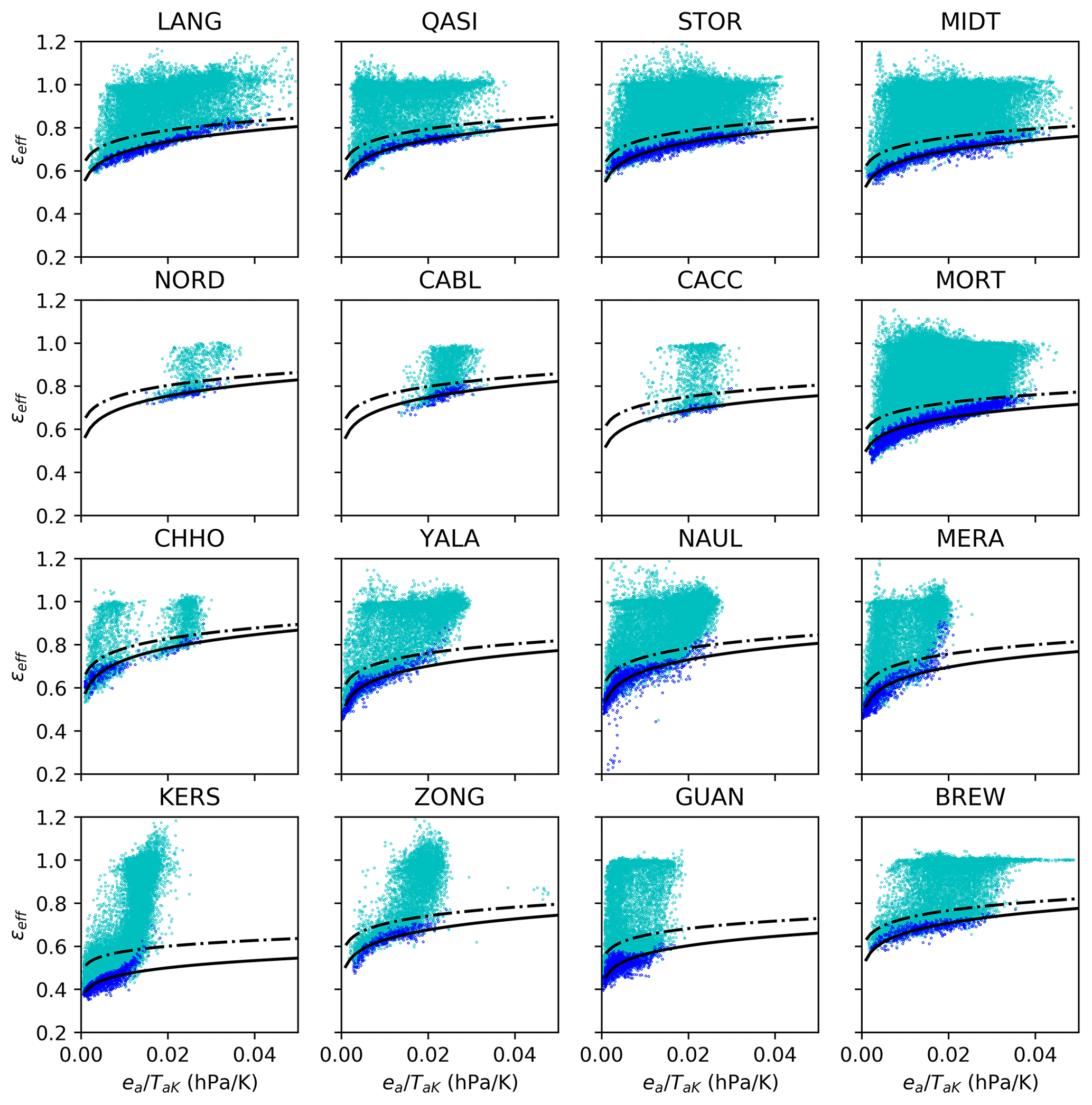
Figure A3Observed εeff (points) and calculated εcs (solid line) fitted to lowest 10 % of LWin in bins (shown in blue). Calculated εeff at clear-sky limit of Nε=0.2 (dash-dotted line).

Figure A4Monthly fraction of clear-sky (light shading), partially cloudy (mid shading) and overcast conditions (dark shading) defined using hourly cloudiness (Nε). Months defined as within the melt season are shaded blue.
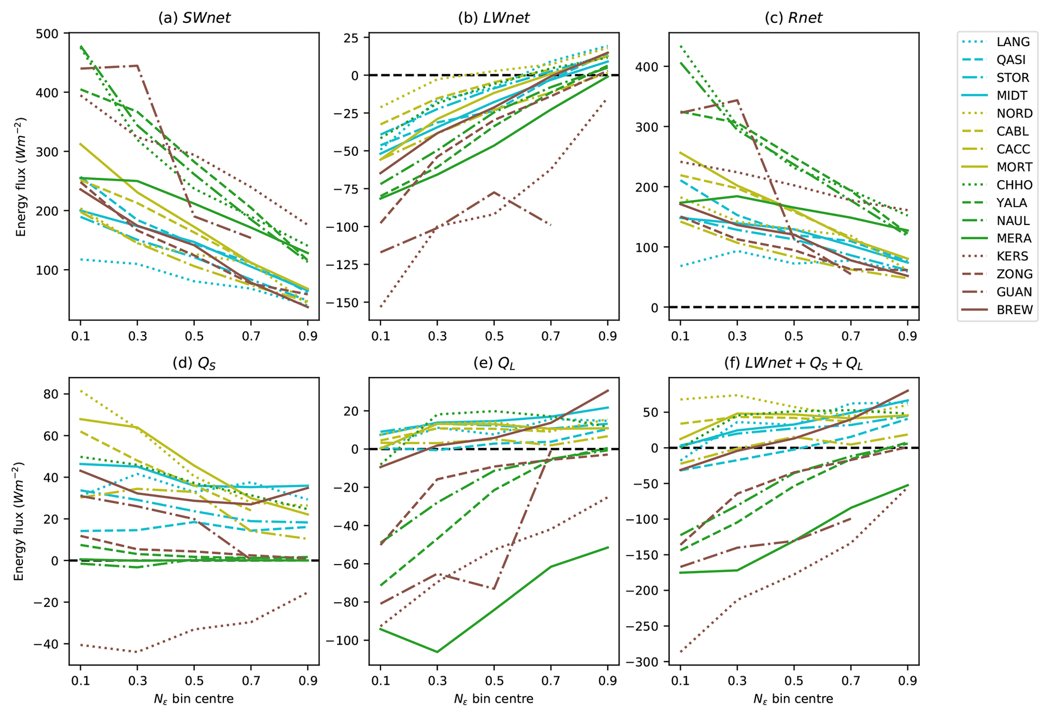
Figure A5Average melt-season SEB terms during hours with surface melt for different cloud conditions (Nε).
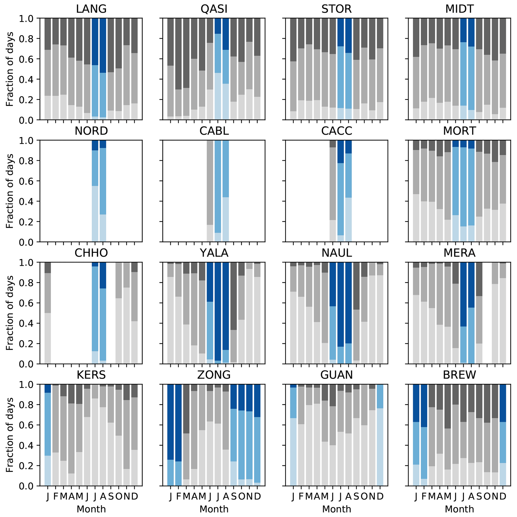
Figure A6As for Fig. 5 but with months with >80 % of maximum monthly average QM shaded blue. Bars show monthly fraction of clear-sky (light shading), partially cloudy (mid shading) and overcast conditions (dark shading) defined using daily average cloudiness (Nε).
AWS data are available from individual paper authors listed in Table 1. Analysis code can be accessed at https://doi.org/10.5281/zenodo.7015997 (Conway, 2022).
JPC conceptualised the study, curated the data, conducted the formal analyses and wrote the paper. Other co-authors supplied data suitable for curation, aided in the investigation and reviewed/edited the paper.
At least one of the (co-)authors is a member of the editorial board of The Cryosphere. The peer-review process was guided by an independent editor, and the authors also have no other competing interests to declare.
Publisher's note: Copernicus Publications remains neutral with regard to jurisdictional claims in published maps and institutional affiliations.
Jonathan P. Conway's contribution to this research was supported by the Royal Society of New Zealand Marsden Fund. The authors wish to thank the following additional people and organisations for data contributions and funding data collection and processing: Maxime Litt, Hans Oerlemans, GLACIOCLIM (UGA-OSUG, CNRS-INSU, IRD, IPEV, INRAE), International Joint Laboratory LMI GREAT-ICE (IRD, EPN Quito), PROMICE, the Greenland Ecosystem Monitoring Programme, ICIMOD, Antoine Rabatel (IGE), Alvaro Soruco (UMSA, Bolivia), a NSERC Discovery Grant and Research Tools and Instruments, and the Canada Foundation for Innovation. Mohd Farooq Azam acknowledges research grants from IFCPAR and IRD, France. Patrick Wagon is thanked for his helpful comments on the paper. We also thank the editor and two anonymous reviewers for their comments, which have improved the final paper.
This research has been supported by the Royal Society of New Zealand Marsden Fund (grant no. NIW1804).
This paper was edited by Caroline Clason and reviewed by two anonymous referees.
Abermann, J., Van As, D., Wacker, S., Langley, K., Machguth, H., and Fausto, R. S.: Strong contrast in mass and energy balance between a coastal mountain glacier and the Greenland ice sheet, J. Glaciol., 65, 263–269, https://doi.org/10.1017/jog.2019.4, 2019.
Ambach, W.: The influence of cloudiness on the net radiation balance of a snow surface with high albedo, J. Glaciol., 13, 73–84, https://doi.org/10.3189/S0022143000023388, 1974.
Andreassen, L. M., Van Den Broeke, M. R., Giesen, R. H., and Oerlemans, J.: A 5 year record of surface energy and mass balance from the ablation zone of Storbreen, Norway, J. Glaciol., 54, 245–258, https://doi.org/10.3189/002214308784886199, 2008.
Azam, M. F., Wagnon, P., Vincent, C., Ramanathan, AL., Favier, V., Mandal, A., and Pottakkal, J. G.: Processes governing the mass balance of Chhota Shigri Glacier (western Himalaya, India) assessed by point-scale surface energy balance measurements, The Cryosphere, 8, 2195–2217, https://doi.org/10.5194/tc-8-2195-2014, 2014.
Azam, M. F., Kargel, J. S., Shea, J. M., Nepal, S., Haritashya, U. K., Srivastava, S., Maussion, F., Qazi, N., Chevallier, P., Dimri, A. P., Kulkarni, A. V., Cogley, J. G., and Bahuguna, I.: Glaciohydrology of the Himalaya-Karakoram, Science, 373, eabf3668, https://doi.org/10.1126/science.abf3668, 2021.
Brutsaert, W.: A Theory for Local Evaporation (or Heat Transfer) From Rough and Smooth Surfaces at Ground, Water Resour. Res., 11, 543–550, https://doi.org/10.1029/WR011i004p00543, 1975.
Buck, A. L. A. L.: New Equations for Computing Vapor Pressure and Enhancement Factor, J. Appl. Meteorol., 20, 1527–1532, https://doi.org/10.1175/1520-0450(1981)020<1527:NEFCVP>2.0.CO;2, 1981.
Chen, J., Du, W., Kang, S., Qin, X., Sun, W., Liu, Y., Jin, Z., Li, Y., and Wang, L.: Eight-year analysis of radiative properties of clouds and its impact on melting on the Laohugou Glacier No. 12, western Qilian Mountains, Atmos. Res., 250, 105410, https://doi.org/10.1016/j.atmosres.2020.105410, 2021.
Church, J. A., White, N. J., Konikow, L. F., Domingues, C. M., Cogley, J. G., Rignot, E., Gregory, J. M., van den Broeke, M. R., Monaghan, A. J., and Velicogna, I.: Revisiting the Earth's sea-level and energy budgets from 1961 to 2008, Geophys. Res. Lett., 38, L18601, https://doi.org/10.1029/2011gl048794, 2011.
Conway, J.: jonoconway/cloud-glacier: v1.0.0 (v1.0.0), Zenodo [code], https://doi.org/10.5281/zenodo.7015997, 2022.
Conway, J. P. and Cullen, N. J.: Cloud effects on surface energy and mass balance in the ablation area of Brewster Glacier, New Zealand, The Cryosphere, 10, 313–328, https://doi.org/10.5194/tc-10-313-2016, 2016.
Conway, J. P., Cullen, N. J., Spronken-Smith, R. A., and Fitzsimons, S. J.: All-sky radiation over a glacier surface in the Southern Alps of New Zealand: characterizing cloud effects on incoming shortwave, longwave and net radiation, Int. J. Climatol., 35, 699–713, https://doi.org/10.1002/joc.4014, 2015.
Conway, J. P., Helgason, W. D., Pomeroy, J. W., and Sicart, J. E.: Icefield breezes: mesoscale diurnal circulation in the atmospheric boundary layer over an outlet of the Columbia Icefield, Canadian Rockies, J. Geophys. Res.-Atmos., 126, e2020JD034225, https://doi.org/10.1029/2020jd034225, 2021.
Cullen, N. J. and Conway, J. P.: A 22 month record of surface meteorology and energy balance from the ablation zone of Brewster Glacier, New Zealand, J. Glaciol., 61, 931–946, https://doi.org/10.3189/2015JoG15J004, 2015.
Cullen, N. J., Anderson, B., Sirguey, P., Stumm, D., Mackintosh, A., Conway, J. P., Horgan, H. J., Dadic, R., Fitzsimons, S. J., and Lorrey, A.: An 11-year record of mass balance of Brewster Glacier, New Zealand, determined using a geostatistical approach, J. Glaciol., 63, 199–217, https://doi.org/10.1017/jog.2016.128, 2016.
Dürr, B. and Philipona, R.: Automatic cloud amount detection by surface longwave downward radiation measurements, J. Geophys. Res., 109, D05201, https://doi.org/10.1029/2003JD004182, 2004.
Fitzpatrick, N., Radić, V., and Menounos, B.: Surface Energy Balance Closure and Turbulent Flux Parameterization on a Mid-Latitude Mountain Glacier, Purcell Mountains, Canada, Front. Earth Sci., 5, 67, https://doi.org/10.3389/feart.2017.00067, 2017.
Fitzpatrick, N., Radić, V., and Menounos, B.: A multi-season investigation of glacier surface roughness lengths through in situ and remote observation, The Cryosphere, 13, 1051–1071, https://doi.org/10.5194/tc-13-1051-2019, 2019.
Giesen, R. H., van den Broeke, M. R., Oerlemans, J., and Andreassen, L. M.: Surface energy balance in the ablation zone of Midtdalsbreen, a glacier in southern Norway: Interannual variability and the effect of clouds, J. Geophys. Res., 113, D21111, https://doi.org/10.1029/2008jd010390, 2008.
Giesen, R. H., Andreassen, L. M., van den Broeke, M. R., and Oerlemans, J.: Comparison of the meteorology and surface energy balance at Storbreen and Midtdalsbreen, two glaciers in southern Norway, The Cryosphere, 3, 57–74, https://doi.org/10.5194/tc-3-57-2009, 2009.
Giesen, R. H., Andreassen, L. M., Oerlemans, J., and Van Den Broeke, M. R.: Surface energy balance in the ablation zone of Langfjordjøkelen, an arctic, maritime glacier in northern Norway, J. Glaciol., 60, 57–70, https://doi.org/10.3189/2014JoG13J063, 2014.
Greuell, W., Knap, W. H., and Smeets, C. J. P. P.: Elevational changes in meteorological variables along a midlatitude glacier during summer, J. Geophys. Res., 102, 25941–25954, 1997.
Hock, R.: Temperature index melt modelling in mountain areas, J. Hydrol., 282, 104-115, https://doi.org/10.1016/s0022-1694(03)00257-9, 2003.
Hock, R., de Woul, M., Radić, V., and Dyurgerov, M.: Mountain glaciers and ice caps around Antarctica make a large sea-level rise contribution, Geophys. Res. Lett., 36, L07501, https://doi.org/10.1029/2008gl037020, 2009.
Hugonnet, R., McNabb, R., Berthier, E., Menounos, B., Nuth, C., Girod, L., Farinotti, D., Huss, M., Dussaillant, I., Brun, F., and Kaab, A.: Accelerated global glacier mass loss in the early twenty-first century, Nature, 592, 726–731, https://doi.org/10.1038/s41586-021-03436-z, 2021.
Huss, M. and Hock, R.: Global-scale hydrological response to future glacier mass loss, Nat. Clim. Change, 8, 135–140, https://doi.org/10.1038/s41558-017-0049-x, 2018.
Huybrechts, P. and Oerlemans, J.: Response of the Antarctic ice sheet to future greenhouse warming, Clim. Dynam., 5, 93–102, https://doi.org/10.1007/BF00207424, 1990.
Konzelmann, T., Van de Wal, R. S. W., Greuell, W., Bintanja, R., Henneken, E., and Abe-Ouchi, A.: Parameterization of global and longwave incoming radiation for the Greenland Ice Sheet, Global Planet. Change, 9, 143–164, 1994.
Kraaijenbrink, P. D. A., Bierkens, M. F. P., Lutz, A. F., and Immerzeel, W. W.: Impact of a global temperature rise of 1.5 degrees Celsius on Asia's glaciers, Nature, 549, 257–260, https://doi.org/10.1038/nature23878, 2017.
Kuipers Munneke, P., Reijmer, C. H., and van den Broeke, M. R.: Assessing the retrieval of cloud properties from radiation measurements over snow and ice, Int. J. Climatol., 31, 756–769, https://doi.org/10.1002/joc.2114, 2011.
Litt, M., Sicart, J. E., Helgason, W. D., and Wagnon, P.: Turbulence Characteristics in the Atmospheric Surface Layer for Different Wind Regimes over the Tropical Zongo Glacier (Bolivia,16∘ S), Bound.-Lay. Meteorol., 154, 471–495, https://doi.org/10.1007/s10546-014-9975-6, 2014.
Litt, M., Shea, J., Wagnon, P., Steiner, J., Koch, I., Stigter, E., and Immerzeel, W.: Glacier ablation and temperature indexed melt models in the Nepalese Himalaya, Sci. Rep.-UK, 9, 5264, https://doi.org/10.1038/s41598-019-41657-5, 2019.
Liu, W., Zhang, D., Qin, X., van den Broeke, M. R., Jiang, Y., Yang, D., and Ding, M.: Monsoon Clouds Control the Summer Surface Energy Balance on East Rongbuk Glacier (6,523 m Above Sea Level), the Northern of Mt. Qomolangma (Everest), J. Geophys. Res.-Atmos., 126, e2020JD033998, https://doi.org/10.1029/2020jd033998, 2021.
MacDonell, S., Kinnard, C., Mölg, T., Nicholson, L., and Abermann, J.: Meteorological drivers of ablation processes on a cold glacier in the semi-arid Andes of Chile, The Cryosphere, 7, 1513–1526, https://doi.org/10.5194/tc-7-1513-2013, 2013.
Mackintosh, A. N., Anderson, B. M., Lorrey, A. M., Renwick, J. A., Frei, P., and Dean, S. M.: Regional cooling caused recent New Zealand glacier advances in a period of global warming, Nat. Commun., 8, 14202, https://doi.org/10.1038/ncomms14202, 2017.
Mandal, A., Angchuk, T., Azam, M. F., Ramanathan, A., Wagnon, P., Soheb, M., and Singh, C.: 11-year record of wintertime snow surface energy balance and sublimation at 4863 m a.s.l. on Chhota Shigri Glacier moraine (western Himalaya, India), The Cryosphere Discuss. [preprint], https://doi.org/10.5194/tc-2021-386, in review, 2022.
Marzeion, B., Kaser, G., Maussion, F., and Champollion, N.: Limited influence of climate change mitigation on short-term glacier mass loss, Nat. Clim. Change, 8, 305–308, https://doi.org/10.1038/s41558-018-0093-1, 2018.
Mernild, S. H., Liston, G. E., and Hiemstra, C. A.: Northern Hemisphere Glacier and Ice Cap Surface Mass Balance and Contribution to Sea Level Rise, J. Climate, 27, 6051–6073, https://doi.org/10.1175/jcli-d-13-00669.1, 2014.
Mölg, T., Cullen, N. J., and Kaser, G.: Solar radiation, cloudiness and longwave radiation over low-latitude glaciers: implications for mass-balance modelling, J. Glaciol., 55, 292–302, https://doi.org/10.3189/002214309788608822, 2009a.
Mölg, T., Cullen, N. J., Hardy, D. R., Winkler, M., and Kaser, G.: Quantifying Climate Change in the Tropical Midtroposphere over East Africa from Glacier Shrinkage on Kilimanjaro, J. Climate, 22, 4162–4181, https://doi.org/10.1175/2009jcli2954.1, 2009b.
Mölg, T., Hardy, D. R., Collier, E., Kropač, E., Schmid, C., Cullen, N. J., Kaser, G., Prinz, R., and Winkler, M.: Mesoscale atmospheric circulation controls of local meteorological elevation gradients on Kersten Glacier near Kilimanjaro summit, Earth Syst. Dynam., 11, 653–672, https://doi.org/10.5194/esd-11-653-2020, 2020.
Niwano, M., Hashimoto, A., and Aoki, T.: Cloud-driven modulations of Greenland ice sheet surface melt, Sci. Rep.-UK, 9, 10380, https://doi.org/10.1038/s41598-019-46152-5, 2019.
Oerlemans, J.: Extracting a climate signal from 169 glacier records, Science, 308, 675–677, https://doi.org/10.1126/science.1107046, 2005.
Oerlemans, J., Giesen, R. H., and van den Broeke, M. R.: Retreating alpine glaciers: increased melt rates due to accumulation of dust (Vadret da Morteratsch, Switzerland), J. Glaciol., 55, 729–736, https://doi.org/10.3189/002214309789470969, 2009.
Pellicciotti, F., Brock, B. W., Strasser, U., Burlando, P., Funk, M., and Corripio, J.: An enhanced temperature-index glacier melt model including the shortwave radiation balance: development and testing for Haut Glacier d'Arolla, Switzerland, J. Glaciol., 51, 573–587, https://doi.org/10.3189/172756505781829124, 2005.
Pellicciotti, F., Raschle, T., Huerlimann, T., Carenzo, M., and Burlando, P.: Transmission of solar radiation through clouds on melting glaciers: a comparison of parameterizations and their impact on melt modelling, J. Glaciol., 57, 367–381, https://doi.org/10.3189/002214311796406013, 2011.
Putnam, A. E., Schaefer, J. M., Denton, G. H., Barrell, D. J. A., Finkel, R. C., Andersen, B. G., Schwartz, R., Chinn, T. J. H., and Doughty, A. M.: Regional climate control of glaciers in New Zealand and Europe during the pre-industrial Holocene, Nat. Geosci., 5, 627–630, https://doi.org/10.1038/ngeo1548, 2012.
Radić, V., Bliss, A., Beedlow, A. C., Hock, R., Miles, E., and Cogley, J. G.: Regional and global projections of twenty-first century glacier mass changes in response to climate scenarios from global climate models, Clim. Dynam., 42, 37–58, https://doi.org/10.1007/s00382-013-1719-7, 2014.
RGI Consortium: Randolph Glacier Inventory – A Dataset of Global Glacier Outlines: Version 6.0: Technical Report, Global Land Ice Measurements from Space, Colorado, USA, Digital Media, https://doi.org/10.7265/N5-RGI-60, 2017.
Sicart, J. E., Wagnon, P., and Ribstein, P.: Atmospheric controls of the heat balance of Zongo Glacier (16∘ S, Bolivia), J. Geophys. Res., 110, D12106, https://doi.org/10.1029/2004jd005732, 2005.
Sicart, J. E., Pomeroy, J. W., Essery, R. L. H., and Bewley, D.: Incoming longwave radiation to melting snow: observations, sensitivity and estimation in Northern environments, Hydrol. Process., 20, 3697–3708, https://doi.org/10.1002/hyp.6383, 2006.
Sicart, J. E., Hock, R., and Six, D.: Glacier melt, air temperature, and energy balance in different climates: The Bolivian Tropics, the French Alps, and northern Sweden, J. Geophys. Res., 113, D24113, https://doi.org/10.1029/2008jd010406, 2008.
Sicart, J. E., Espinoza, J. C., Quéno, L., and Medina, M.: Radiative properties of clouds over a tropical Bolivian glacier: seasonal variations and relationship with regional atmospheric circulation, Int. J. Climatol., 36, 3116–3128, https://doi.org/10.1002/joc.4540, 2016.
van den Broeke, M. R., Smeets, C. J. P. P., Ettema, J., Kuipers Munneke, P., Smeets, P., Ettema, J., and Munneke, P. K.: Surface radiation balance in the ablation zone of the west Greenland ice sheet, J. Geophys. Res., 113, D13105–D13105, https://doi.org/10.1029/2007JD009283, 2008.
van den Broeke, M. R., Smeets, C. J. P. P., and van de Wal, R. S. W.: The seasonal cycle and interannual variability of surface energy balance and melt in the ablation zone of the west Greenland ice sheet, The Cryosphere, 5, 377–390, https://doi.org/10.5194/tc-5-377-2011, 2011.
Van Tricht, K., Lhermitte, S., Lenaerts, J. T., Gorodetskaya, I. V., L'Ecuyer, T. S., Noel, B., van den Broeke, M. R., Turner, D. D., and van Lipzig, N. P.: Clouds enhance Greenland ice sheet meltwater runoff, Nat. Commun., 7, 10266, https://doi.org/10.1038/ncomms10266, 2016.
Zekollari, H., Huss, M., and Farinotti, D.: Modelling the future evolution of glaciers in the European Alps under the EURO-CORDEX RCM ensemble, The Cryosphere, 13, 1125–1146, https://doi.org/10.5194/tc-13-1125-2019, 2019.
Zemp, M., Huss, M., Thibert, E., Eckert, N., McNabb, R., Huber, J., Barandun, M., Machguth, H., Nussbaumer, S. U., Gartner-Roer, I., Thomson, L., Paul, F., Maussion, F., Kutuzov, S., and Cogley, J. G.: Global glacier mass changes and their contributions to sea-level rise from 1961 to 2016, Nature, 568, 382–386, https://doi.org/10.1038/s41586-019-1071-0, 2019.