the Creative Commons Attribution 4.0 License.
the Creative Commons Attribution 4.0 License.
 | 25 Jan 2022
Sources of uncertainty in Greenland surface mass balance in the 21st century
Katharina M. Holube
Tobias Zolles
Andreas Born
The surface mass balance (SMB) of the Greenland ice sheet is subject to considerable uncertainties that complicate predictions of sea level rise caused by climate change. We examine the SMB of the Greenland ice sheet in the 21st century with the Bergen Snow Simulator (BESSI) surface energy and mass balance model. To estimate the uncertainty of the SMB, we conduct simulations for four greenhouse gas emission scenarios using the output of a wide range of Earth system models (ESMs) from the sixth phase of the Coupled Model Intercomparison Project (CMIP6) to force BESSI. In addition, the uncertainty of the SMB simulation is estimated by using 16 different parameter sets in our SMB model. The median SMB across ESMs and parameter sets, integrated over the ice sheet, decreases over time for every emission scenario. As expected, the decrease in SMB is stronger for higher greenhouse gas emissions. The regional distribution of the resulting SMB shows the most substantial SMB decrease in western Greenland for all ESMs, whereas the differences between the ESMs are most pronounced in the north and around the equilibrium line. Temperature and precipitation are the input variables of the snow model that have the largest influence on the SMB and the largest differences between ESMs. In our ensemble, the range of uncertainty in the SMB is greater than in previous studies that used fewer ESMs as forcing. An analysis of the different sources of uncertainty shows that the uncertainty caused by the different ESMs for a given scenario is larger than the uncertainty caused by the climate scenarios. In comparison, the uncertainty caused by the snow model parameters is negligible, leaving the uncertainty of the ESMs as the main reason for SMB uncertainty.
- Article
(9446 KB) - Full-text XML
- BibTeX
- EndNote


The Greenland ice sheet (GrIS) currently experiences a net mass loss through changes in surface mass balance (SMB) and dynamical processes such as solid ice discharge. In 2005–2017, the GrIS contributed almost as much to sea level rise as all glaciers worldwide (Sasgen et al., 2020). There is substantial uncertainty in the magnitude of sea level rise that will be caused by the GrIS in the future (Goelzer et al., 2020). According to Slater et al. (2020), the contribution of melt to sea level rise in 2007–2017 exceeded the highest estimates of the IPCC Fifth Assessment Report sea level predictions, whereas for dynamic ice loss the lower or middle estimates were met. The influence of SMB on the total mass loss becomes more important in the future because outlet glaciers will retreat above sea level (Fettweis et al., 2013). The uncertainty in ice discharge is not as substantial as the uncertainties of climate projections and in SMB (Aschwanden et al., 2019).
SMB simulations are subject to uncertainty from multiple sources, such as the spatial resolution of the ice sheet model, the parametrization of processes like melt–albedo feedback and the forcing of the SMB model (Goelzer et al., 2013). The latter can be separated into the uncertainty about the radiative forcing pathway (hereafter, climate scenario), and the climate projection uncertainty, which can be assessed with projections of different Earth system models (ESMs), although their similarities limit the validity of this approach (Knutti et al., 2013). The influence of climate projection uncertainty on the SMB of the GrIS has been simulated with SMB models of different complexities. Positive degree-day (PDD) models apply an empirical relationship between melt and temperature. Several ESMs from the third generation of the Coupled Model Intercomparison Project (CMIP3) have been used to force an ice sheet model in which the SMB is calculated by the PDD method (Graversen et al., 2011). Yan et al. (2014) employed another ice sheet model that also uses the PDD method for the SMB calculations and forced it with CMIP5 ESMs. However, PDD models are calibrated to match the present state of the climate and so their validity in a warming climate is limited (Vizcaino, 2014). This is less of a concern in regional climate models (RCMs) coupled with a snow model where many physical processes are resolved. These are used to downscale ESM simulations, which often do not have the spatial resolution needed to simulate the SMB with sufficient accuracy. However, RCMs are expensive, limiting their use to downscaling only a few ESMs (Fettweis et al., 2008; Franco et al., 2011; Fettweis et al., 2013; Hanna et al., 2020). Fettweis et al. (2008) utilized RCM simulations forced with a subset of CMIP3 simulations and performed a multilinear regression for the SMB changes as a function of temperature and precipitation to calculate the SMB changes for CMIP3 models not used as forcing. For CMIP6, Hanna et al. (2020) simulated the SMB of Greenland using the output of five ESMs. Hofer et al. (2020) showed that the predicted climate from these representatively selected ESMs leads to a larger GrIS SMB decrease in CMIP6 than in CMIP5. While their results already include some variability between ESMs, their selection from the CMIP6 model pool is necessarily incomplete, and the relative importance of climate simulation as compared with other sources of uncertainty remains unclear.
We address some of those open questions in this study with the surface energy and mass balance model Bergen Snow Simulator (BESSI) (Born et al., 2019; Zolles and Born, 2021), which simulates energy exchange processes at the snow or ice surface and is therefore more physically correct than PDD models, while requiring fewer computational resources than RCMs. To assess the uncertainty of the radiative forcing, we consider four climate scenarios that lead to different extents of climate change. We simulate the SMB for these climate scenarios using the output of 26 ESMs from CMIP6 to take into account the uncertainty of climate projections. To estimate the uncertainty of the parametrization, we conduct all simulations with 16 sets of parameters for BESSI (Born et al., 2019; Zolles and Born, 2021). While this approach cannot substitute a comparison of different SMB models as in Fettweis et al. (2020), it enables us to assess the relative importance of climate- and snow-related parameters in a coherent framework. We compare the different uncertainties and study spatial variations in the simulated SMB and the importance of the different input variables in different parts of Greenland (Sect. 3) after a description of our methods (Sect. 2). Finally, we compare our results to previous studies (Sect. 4).
2.1 Snow model
The Bergen Snow Simulator (BESSI) (Born et al., 2019; Zolles and Born, 2021) is a surface energy and mass balance model for glaciated regions with a flexible spatial domain. In this study, the domain is Greenland with an equidistant resolution of 10 km. The topography of the ice sheet is based on ETOPO1 (Amante and Eakins, 2009) and remains fixed throughout the simulations. The vertical dimension consists of up to 15 snow or firn layers that are adjusted by splitting or merging layers depending on the snow mass in each grid cell (Born et al., 2019; Zolles and Born, 2021). The five daily input variables are air temperature and dew point at 2 m above ground, the amount of precipitation, and surface downwelling shortwave and longwave radiation. The top layer changes its mass and energy according to the forcing of the input variables. Precipitation falls as snow when the air temperature is below 0 ∘C and as rain otherwise. Meltwater percolates down into deeper layers and refreezes. Horizontal exchanges of mass or energy are deemed negligible on the 10 km grid. When there is no more snow left to melt, the excess energy is used to melt ice. Corrections are made when the melt exceeds the existing amount of ice (Appendix A). For a detailed description of the snow model, see Born et al. (2019) and Zolles and Born (2021). The performance of BESSI has been compared with other SMB models in Fettweis et al. (2020). Although snowfall and runoff are lower in BESSI than in other SMB models, the SMB and its trend are consistent with most other studied models because both biases cancel each other out.
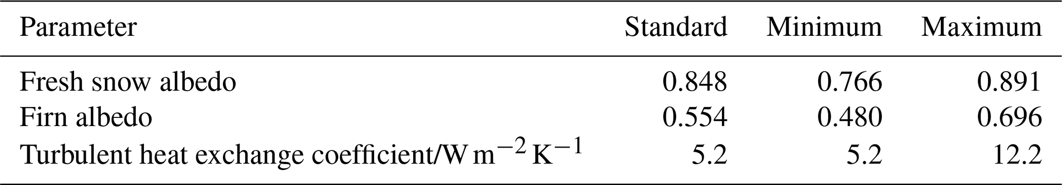
BESSI uses parameterizations of several physical processes. In this study, we vary the albedo and turbulent heat exchange parameters (Table C1), which contribute to the parameter uncertainty discussed below. The albedo changes caused by ageing of the snow are parameterized depending on temperature, whereas the ageing is accelerated at 0 ∘C depending on the liquid water content (Bougamont et al., 2005; Zolles and Born, 2021). Thus, the albedo of the snow can take values between the prescribed albedos of fresh snow and firn. Ice is assigned a separate albedo. The turbulent sensible heat flux depends on the difference between air and surface temperature, and on the turbulent heat exchange coefficient, which is a model parameter describing both changes in wind speed and efficiency of the turbulent exchange (Zolles and Born, 2021).
The model parameters of BESSI are calibrated to the RACMO SMB (Noël et al., 2016). Here, we use an ensemble of equally plausible model parameter settings based on a multivariate calibration (Zolles et al., 2019). For the calibration, BESSI was run for 500 years with ERA-Interim (Dee et al., 2011) as forcing data using different parameter combinations. The performance of the simulation is compared to the RACMO SMB over the period 1979–2017 on an annual basis. We are using seven measures of goodness of fit, based on the bias, the mean absolute deviation (MAD), and the root-mean-square error (RMSE) of the SMB. The bias is the difference between the ice-sheet-wide integrated SMB between RACMO and BESSI, while we calculate three representations of RMSE and MAD. The first calculates the Greenland-wide SMB and its temporal MAD over the years, the second calculates a temporal MAD for each grid point and averages them over all grid points, with the third and final being the MAD over all points in space and time. A similar approach is used for the RMSE. In total we are using seven objective functions for the multivariate optimization. We evaluate the performance of BESSI relative to all the objective functions. In a non-ideal world not all objectives can be minimized simultaneously. This yields multiple equally plausible optimal solutions, where one objective function can not be improved without compromising another. The ensemble of these optimal solutions is referred to as Pareto optimal set. Similar to the method used by Zolles et al. (2019), we calculate the Pareto optimal set. This yields a total of 16 different solutions whose parameter ranges are given in Table C1.
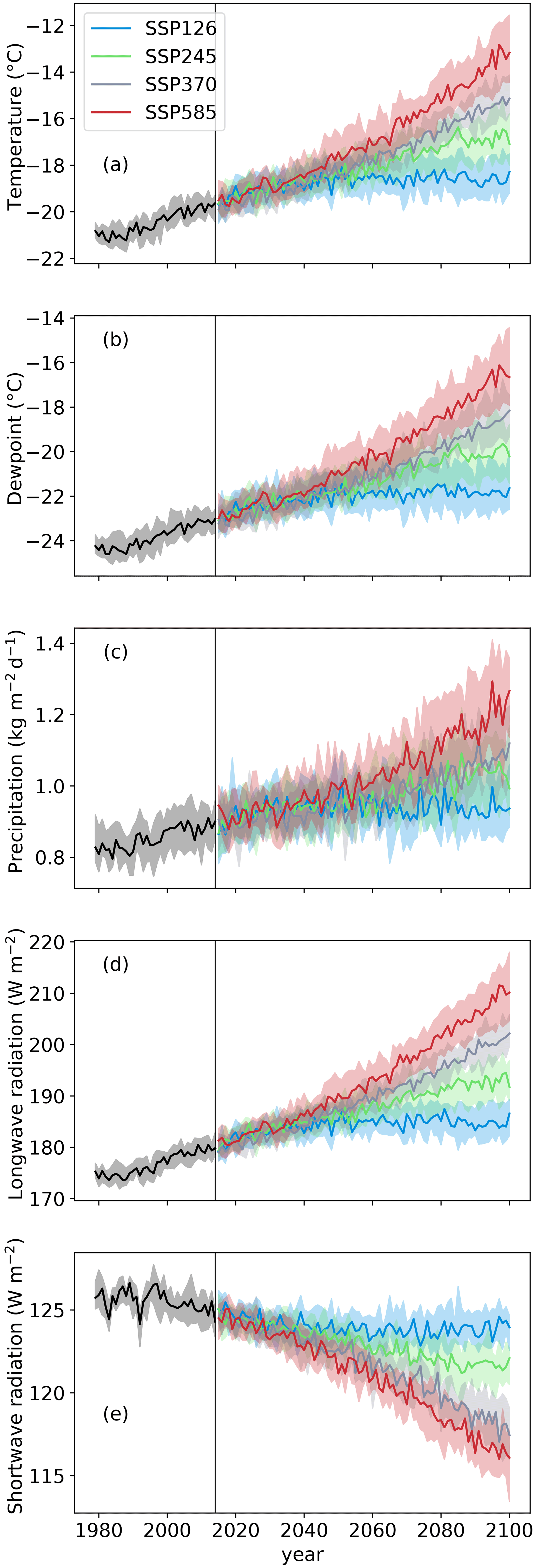
Figure 1Input variables for BESSI, which are interpolated and bias-corrected ESM data, for different scenarios, averaged over the Greenland ice sheet. The solid line is the median over all ESMs for one scenario, and the shaded area between the 25 % and 75 % percentiles represents half of the ESMs. (a) Temperature at 2 m above ground. (b) Dew point at 2 m above ground. (c) Amount of precipitation. (d) Surface downwelling longwave radiation. (e) Surface downwelling shortwave radiation. The vertical line indicates the boundary between the common time period of the historical ESM simulations and ERA-Interim (1979–2014) and the future projection time period (from 2015). Please note that the precipitation unit, 1 , equals 1 mm (w.e.) per day; w.e. stands for water equivalent.
2.2 Earth system models
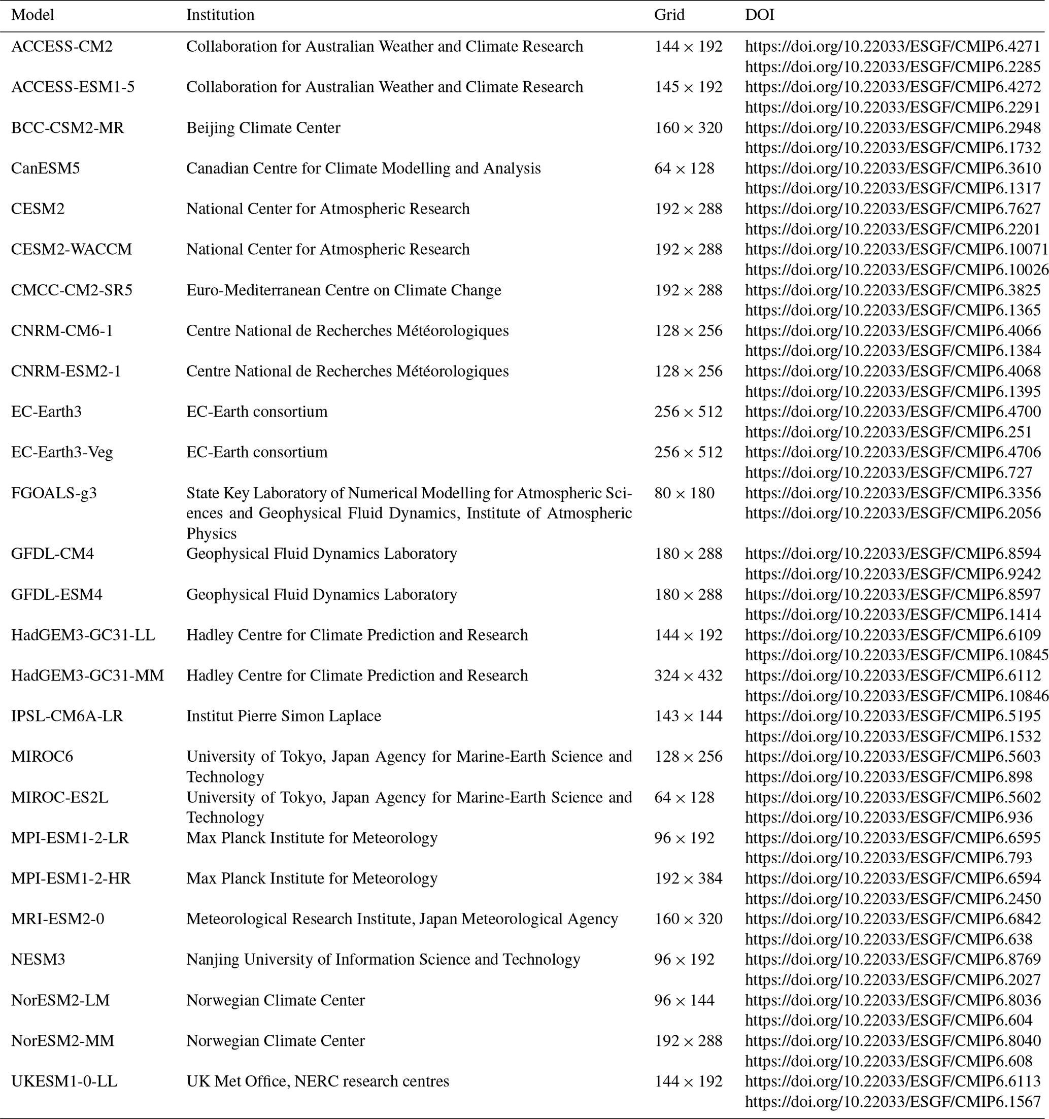
We use ESM output of CMIP6 for the period of 2015–2100 (Eyring et al., 2016). The Tier 1 scenarios (with increasing radiative forcing: SSP126, SSP245, SSP370, and SSP585) from ScenarioMIP are selected for this study because they encompass a wide range of future forcing possibilities (O'Neill et al., 2016) and are available for many different ESMs. We selected 26 ESMs that provide all of BESSI's input variables for at least two scenarios (Appendix Table B1), with the exception of the dew point, which is calculated from the relative humidity if necessary.
The input variables are interpolated linearly to the 10 km BESSI grid. ESM biases are calculated based on the delta method (Beyer et al., 2020) by comparing the daily mean of the historical simulation and the daily mean of the ERA-Interim reanalysis in the period of 1979–2014, in which both datasets are available. For all input variables except precipitation, the differences between the daily means are subtracted from the future projection. These differences also include discrepancies in topography, so the dependence of, for example, temperature on elevation is accounted for in the additive bias correction. As mentioned in Sect. 2.1, BESSI uses ETOPO1 and accounts for the differences with the ERA-Interim topography by performing a correction with a constant moist adiabatic lapse rate. Precipitation is bias corrected by the ratio of ERA-Interim and historical mean precipitation because its high variability would lead to negative values if the difference was used. During the winter, shortwave radiation may be very weak so that the bias correction can lead to localized, small negative values. These values are set to zero. The daily means of precipitation are affected by individual intense precipitation events due to the short length of the historical period. The monthly biases are less affected by these events, and therefore we multiply the projected precipitation with the ratio of the monthly mean precipitation of the historical reference and the reanalysis data to perform bias correction instead of the daily means.
Throughout the 21st century, the median air temperature over all ESMs rises in every scenario except in the scenario with the smallest increase in greenhouse gases (SSP126), where it remains almost constant during the second half of the century (Fig. 1a). While shortwave radiation decreases slightly, precipitation, longwave radiation, and dew point increase over the course of the century (Fig. 1b–e). The stronger the greenhouse gas forcing, the larger the change in these variables. For each variable except precipitation, there are distinct differences in ESM medians between all scenarios at the end of the century, and the differences between scenarios are of similar magnitude to the interquartile ranges. The trends in precipitation are weaker compared to the ranges of values between the ESMs.
2.3 Simulations and ensemble design
We conduct two different kinds of SMB simulations. (i) In the main ensemble, the forcing data for four climate scenarios are taken from different ESMs, and the snow model parameters are varied. It illustrates the temporal and spatial behaviour of the SMB and it enables us to separate the different uncertainty components. (ii) The “single-forcing” ensemble shows the influence of the individual input variables.
The main ensemble uses 96 selected ESM–scenario combinations (Table B1). In addition, we conduct 26 simulations for the historical reference period (1979–2014), i.e. one for each ESM. Each of the simulations is conducted with 16 different snow model parameter sets, resulting in 1952 simulations. The selection process of the parameter combinations is described in Sect. 2.1. The firn cover is initialized by forcing BESSI with ERA-Interim reanalysis data for 540 years, to reach a dynamically and thermodynamically stable firn cover at the year 2014. The long response time of the firn cover requires an initialization period of several hundred years, which is realized by forcing the model with the ERA-Interim data 15 times back and forth (Zolles and Born, 2021). For the historical time period, the initialization ends in 1979 after 14 ERA-Interim cycles back and forth. For every parameter set, the same initialized firn cover is used to save computation time, but the bias caused by this inconsistency is generally overcompensated after a few years of climate forcing.
In the single-forcing simulations, the transient ESM simulations are used as input for only one variable, and the daily ERA-Interim climatology is used for the others to assess the influence of each variable on the SMB. The scenario SSP585 is chosen because it is available for all 26 ESMs, and we used the snow model parameter set that produces the best results in the calibration with RACMO (Sect. 2.1). For precipitation, the daily ERA-Interim climatology cannot be used as it overestimates the surface albedo due to unrealistic small amounts of snowfall every day (Sodemann et al., 2008). This leads to an overestimation of the mass balance of up to 40 % (Zolles and Born, 2022). Instead we use the monthly precipitation climatology and distribute the ERA-Interim monthly average following the temporal distribution of precipitation in the ESM simulation:
where P stands for precipitation, “m” stands for monthly mean, “d” stands for daily mean, and year stands for the point in time of the simulation. Therefore, the climatological daily precipitation distribution differs for each ESM, but the monthly averages are identical. For each of the 26 ESMs, we conducted six simulations for the SMB: a reference simulation with the historical climatology and five simulations with different transient variables (air and dew point temperature, precipitation, shortwave and longwave radiation). We need a separate reference simulation for each ESM because the precipitation distribution differs for each ESM according to Eq. (1).
3.1 Scenario surface mass balance simulations
In this section, we show temporal and spatial differences between the ESMs and climate scenarios of the median SMB over all parameter combinations. The median SMB at the end of the century over the ESMs and snow model parameters is shown for the different climate scenarios in Table 1. The surface mass balance decreases relative to the historical simulations in all scenarios (Fig. 2). In the moderate scenario SSP126, the SMB is relatively stable to the end of the century. Higher emissions of greenhouse gases (stronger forcing) lead to a lower SMB (SSP245, SSP370, SSP585). With stronger warming, the range in simulated SMB for different ESMs increases, although the range in input variables except precipitation does not seem to depend on the scenario (Fig. 1). For precipitation, the interquartile range between the ESMs increases only slightly with stronger greenhouse gas forcing. Precipitation variability alone cannot explain the larger interquartile range in SMB in the warmer scenarios. The reason for the increasingly dissimilar SMBs with stronger greenhouse gas forcing is that larger changes in the input variables have a larger cumulative effect on the SMB (Sect. 3.3).
Table 1Median and quartiles over all ESM and snow model parameter combinations of the 2091–2100 SMB mean value for different scenarios.
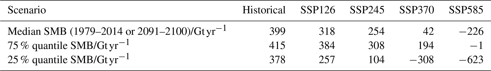
When BESSI is forced with ERA-Interim data (Fig. 2, orange), a relatively low SMB in the early 21st century is apparent. This correlates with more frequent Greenland blocking (Sasgen et al., 2020). A similar reduction in SMB is not observed when forcing BESSI with historical ESM data (Fig. 2, black) because the coarse horizontal resolution hampers the representation of the observed blocking and its increased activity (Davini and D’Andrea, 2020).
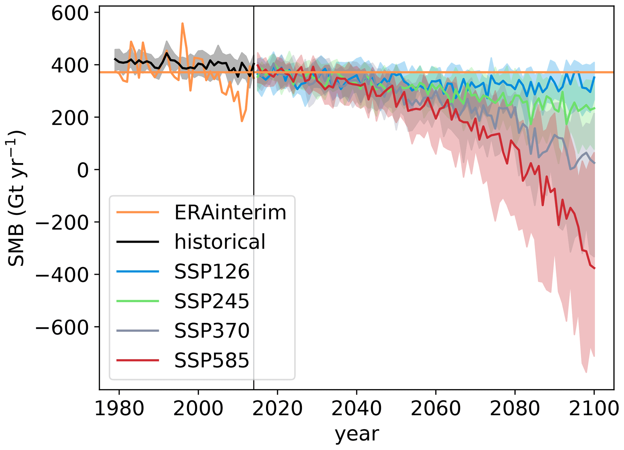
Figure 2Surface mass balance simulations forced with ERA-Interim reanalysis data, historical ESM simulations, and scenario climate simulations, given as the median over the SMB for all snow model parameter combinations. The solid line is the median of all ESMs, and the shading shows the 25 % and 75 % percentiles. Orange represents SMB forced with ERA-Interim, and the horizontal line is its mean value.
Spatial anomalies for the last decade of the SMB in the low-emission scenario SSP126 and the high-emission scenario SSP585 are shown in Fig. 3. In the west of Greenland, the SMB in the 2090s is lower than in ERA-Interim (1979–2014), independent of the scenario (Fig. 3a and b). In this region, higher temperatures lead to increased melt. In the centre of the ice sheet, the SMB is slightly higher than in ERA-Interim, especially in the southeast. There, heavier precipitation occurs under a warmer climate. However, the SMB increase in the centre is outweighed by the SMB decrease at the margin of the ice sheet. These SMB changes are much more pronounced in the high-end scenario SSP585 because of the enhanced change in the input variables. Currently observed SMB changes are dominated by amplified melting in the west and by snowfall in the east (Sasgen et al., 2020). In the north, the temperatures are too low for much melt at the present day, but with an average increase of temperature over the ice sheet of approximately 6 K in SSP585 (Fig. 1a), melt increases considerably there.
Figure 3Anomaly of the median SMB over all parameter combinations (2090–2099 mean) with respect to ERA-Interim (1979–2014 mean) (a, b) with standard deviation (c, d) and relative standard deviation (e, f) for the scenarios SSP126 (a, c, e) and SSP585 (b, d, f). (a, b) The contour line indicates a mass balance of zero. Note the different scales for positive and negative values. (e, f) In the shaded area, the absolute value of the surface mass balance is smaller than 50 kg m−2, which is considered to be close to zero, and thus the relative standard deviations are invalid.
At the margin of the ice sheet, the standard deviation of the SMB between the ESMs is largest (Fig. 3c and d). The relative standard deviation of the SMB reaches the highest values near the equilibrium line (Fig. 3e and f), and thus the choice of ESM is decisive for the SMB in this region. In the high-emission scenario SSP585, the equilibrium line is subject to substantial uncertainty, which is greater than in the moderate scenario SSP126 (Fig. 4). Equilibrium line changes show that the differences between ESMs driven by the same scenario increase with stronger greenhouse gas forcing (Fig. 2).
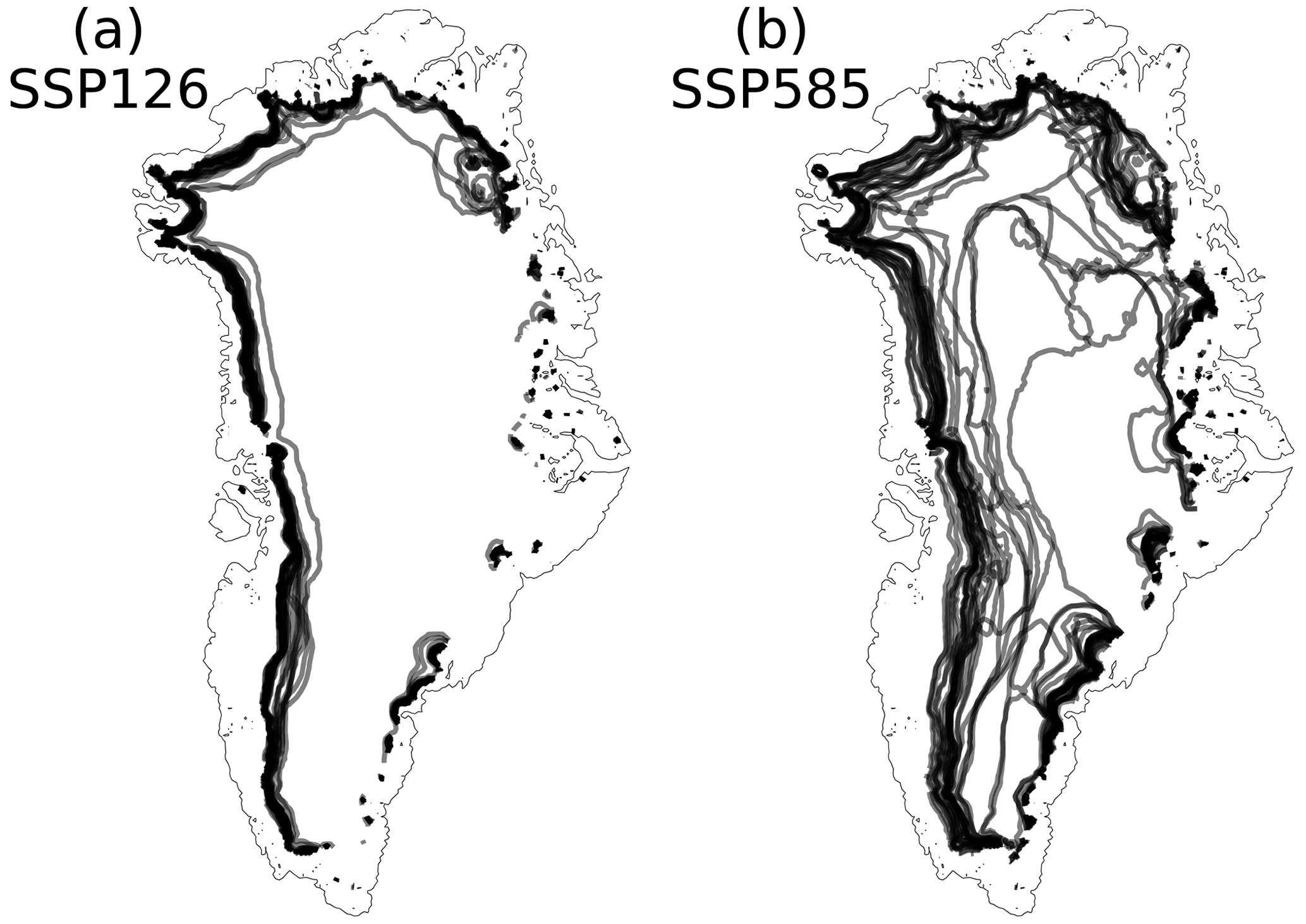
Figure 4Equilibrium lines of the median SMB over all parameter combinations (temporal mean for the period of 2090–2099) for different ESMs and the scenarios SSP126 (a) and SSP585 (b).
3.2 Estimation of uncertainties
Having examined the spatial variations between ESMs, we next study the variance of the full ensemble containing ESMs, emission scenarios and snow model parameters. We split the variance in spatially integrated SMB over all simulations into four different components using a method based on Hawkins and Sutton (2009) and described in more detail in Appendix C: a fourth degree polynomial fit is applied to the decadal running mean of spatially integrated SMB for each individual simulation to separate trends from variations on small timescales. The residuals of the fits are considered the internal variability of the system, for example fluctuations in SMB caused by alternating dry and wet periods. The law of total variance is applied to the whole ensemble of polynomials to split the total variance into three independent components for each year. These components are the variances caused by ESMs, climate scenarios, and BESSI parameters (albedo of fresh snow and firn, turbulent heat exchange coefficient). These variances quantify three relevant sources of uncertainty, with internal variability being the fourth.
The sum of the different uncertainty components increases strongly over the course of the century (Fig. 5a). The relative contributions of the different uncertainty components are shown in Fig. 5b by normalizing with the sum of all components. In the first years of the simulations, the internal variability is the largest source of uncertainty, showing that it is most important in the absence of external forcing. While the scenario uncertainty has the smallest contribution in the beginning, its importance increases in the second half of the century, as decarbonization measures and the adaption of the climate system take time (Davy and Outten, 2020). The parameter uncertainty is slightly larger than the scenario uncertainty at first, but its relative importance decreases over time. Its overall small contribution to uncertainty indicates that the results of our SMB simulations are almost independent of the specific parameter combination of BESSI. The parameter uncertainty does not depict the total snow model uncertainty because the approach to calculate the SMB is the same regardless of the parameter combination, whereas differences in the ESMs are caused by different ways of simulating the processes. The spatial resolution necessarily contributes to the uncertainty in SMB modelling because elevation and associated temperature differences on the sub-grid scale can lead to unrealistically high temperatures prescribed above the ablation zone, reducing the SMB (Goelzer et al., 2013). Furthermore, the calculation of precipitation and runoff is less accurate in BESSI compared to other snow models, and these biases could increase in a warming climate (Fettweis et al., 2020), which is not represented in the parameter uncertainty either.
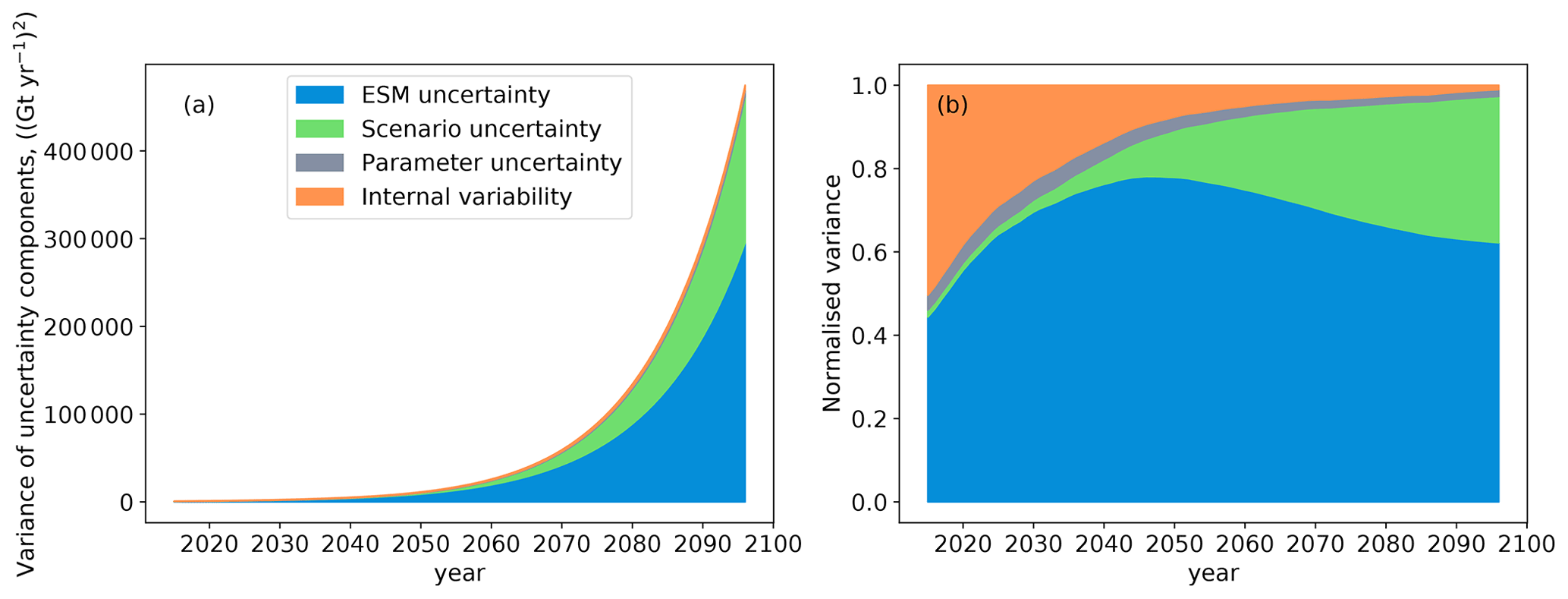
Figure 5(a) Total and (b) relative variances of the different uncertainty components: choice of ESM (blue), different emission scenarios (green), different snow model parameters (grey), and internal variability (orange). The time period does not extend to 2100 because the variance splitting approach is applied to the decadal running means of the yearly SMB.
A few years into the simulation, the ESM uncertainty becomes the largest contributor to the uncertainty and the share of the internal variability decreases rapidly. However, our uncertainty quantification may erroneously attribute a part of the internal variability of the climate simulations to ESM uncertainty (Lehner et al., 2020). In order to estimate this error, we forced BESSI with 10 different realizations of the ESM ACCESS-ESM1-5 (Table B1) and applied the method of Hawkins and Sutton (2009) by replacing the different ESMs with the different realizations of a single ESM. This shows a non-negligible bias in the attribution of the uncertainty in the first decades, up to 35 %, adding a caveat to the relative uncertainties in Fig. 5b for this time period. Note, however, that multiple realizations are available for only about half of the ESMs, and thus we cannot systematically investigate this effect. More importantly for the results of this study, the method bias is small at the end of the century, which means that the ESM uncertainty is robustly shown to be greater than the scenario uncertainty. In other words, in the scenarios with strong forcing, there are some ESMs that induce only small SMB changes, while other ESMs lead to a much stronger SMB decrease. This pronounced uncertainty is larger than the differences between the medians over the ESMs for each scenario. At the end of the century, the ESM uncertainty is about 62 % and the scenario uncertainty is about 35 % of the total variance, whereas the snow model parameter uncertainty and the internal variability represent about 3 % combined.
The separation of variances can be generalized to every grid cell of the GrIS. The total variance of the 1952 simulations is largest at the margin of the ice sheet, where the SMB changes considerably (Fig. 6a and b). The total variance increases by several orders of magnitude from the middle to the end of the century. At the middle of the century, the ESM uncertainty is the most important component at the margin and in the centre of the ice sheet (Fig. 6c). Only in the north and at higher altitudes in the west is the internal variability at its largest. Compared to the other components, the scenario uncertainty is insignificant at the middle of the century (Fig. 6e). At the end of the century, the scenario uncertainty becomes more pronounced, especially at the western margin, where the amount of melt differs considerably between the scenarios (Fig. 6d). The area where the ESM uncertainty has the largest share increases even more at the end of the century, mainly at the expense of the regions where the internal variability is important at the middle of the century. The scenario uncertainty is of similar magnitude as the ESM uncertainty only at the margins of the ice sheet and in the area where the total variance is low.
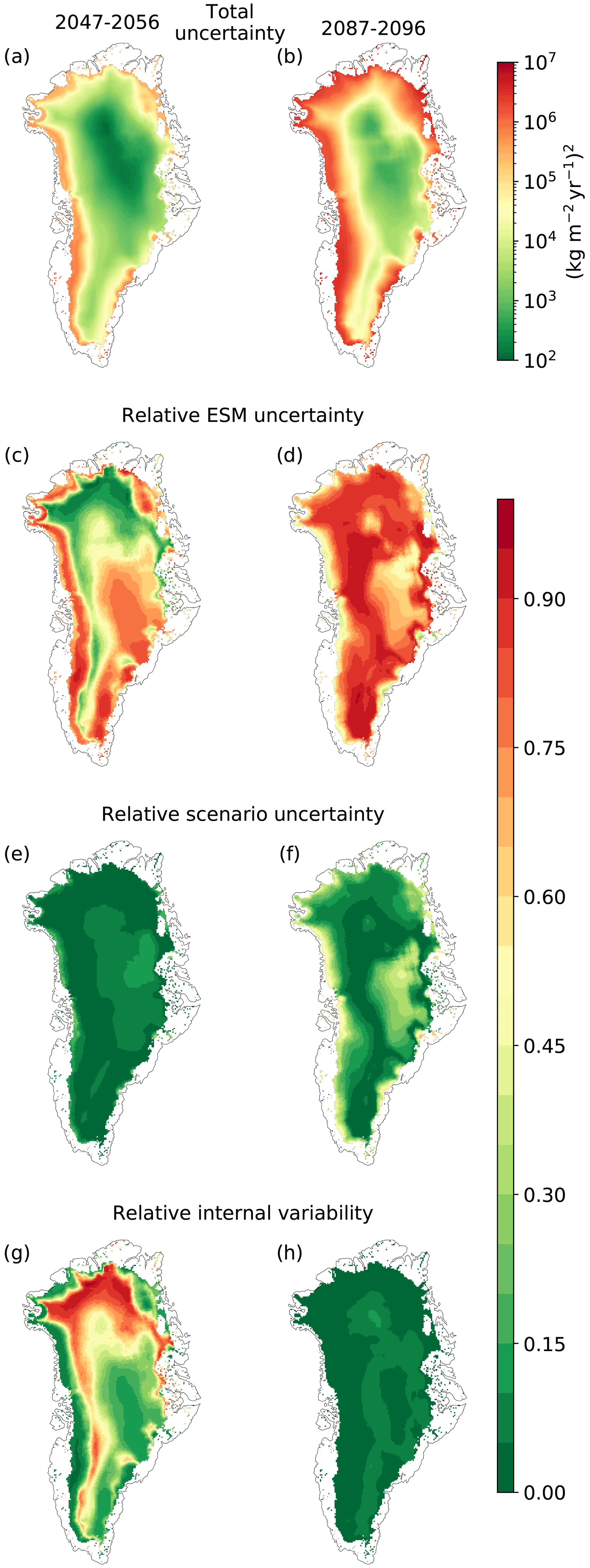
Figure 6(a, b) Total variance, consisting of ESM uncertainty, scenario uncertainty, snow model parameter uncertainty, and internal variability. (c, d) Ratio of ESM uncertainty and sum of the uncertainties. (e, f) Ratio of scenario uncertainty and sum of the uncertainties. (g, h) Ratio of internal variability and sum of the uncertainties. Panels (a, c, e, g) show the mean over the years 2047–2056, panels (b, d, f, h) show the mean over the years 2087–2096. The latter is the last decade that the variance splitting approach is valid for because it is applied to the decadal running mean of the yearly SMB. The years 2047–2056 are chosen as a decade in the middle of the 21st century.
3.3 Single-forcing and regional analysis
In the single-forcing simulations, we run the snow model using only one input variable from each CMIP model simulation. This variable is hereafter called the transient variable. For the other variables, daily means of the historical period of ERA-Interim data are used in the simulation, except for precipitation, whose temporal distribution is again adapted as described in Sect. 2.3. We study the influence of the different input variables on the SMB across the entire GrIS and show three regions previously used by Zolles and Born (2021) (Fig. 7). These regions are selected because they illustrate the spatial differences in the behaviour of the SMB.
The SMB increases when precipitation is the transient variable due to an increase in snowfall (Fig. 1c). In the simulation with transient dew point, the SMB also increases through an increase in desublimation, but the effect is smaller. When the downwelling longwave radiation increases, the snow temperature rises, which leads to more melt. The effect of melting caused by increased air temperature is stronger than that of increased longwave radiation except for the east where the SMB change is dominated by precipitation changes. The interquartile range is largest when temperature or precipitation are the transient variables, except for the east where the dew point has a larger interquartile range than the temperature. Consequently, these variables dominate the uncertainty of the SMB simulations. Shortwave radiation alone has a negligible influence on the SMB in the idealized experiments performed. This does not agree with Hofer et al. (2017), who found a link between amplified melt and recent increases in shortwave radiation through shifts in North Atlantic Oscillation and Greenland blocking. However, the ESMs used in this study predict a decrease in shortwave radiation, which could explain the disagreement. In addition, Greenland blocking is not well represented in ESMs (Davini and D’Andrea, 2020).
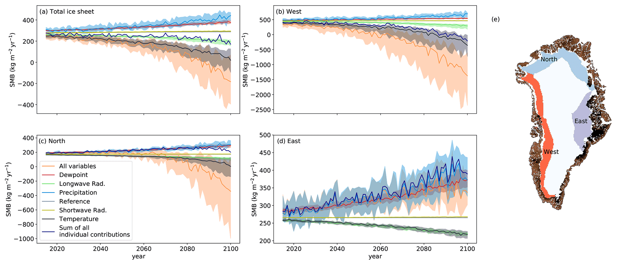
Figure 7SMB for single-forcing simulations for the entire GrIS (a) and selected regions (b–d). The variable named in the legend is transient for scenario SSP585, while all other variables are the ERA-Interim mean. “All variables” indicates that all variables are transient (the same as Fig. 2). “Reference” shows the historical climatology for all variables with precipitation distribution as in CMIP. (e) Positions of the selected regions. Regions “north” and “west” are at elevations of 1000–2000 m. The southeast is precipitation driven and the change in SMB with altitude is less developed; therefore, the region “east” is at elevations of 1000–3000 m.
The sum of all individual changes does not equal the fully transient simulation driven by the SSP585 scenario (Fig. 7). This highlights non-linearities that amplify the SMB reduction. For example, air temperature and precipitation often covary so that the increased precipitation compensates the increased melt only partly. If heavier precipitation delivers more rain, the energy required to refreeze the additional rain in the snowpack increases its heat. We conclude that when air temperature and longwave radiation rise together in a warmer and cloudier future and more energy is available at the surface and due to the non-linearity of the SMB, increased melt is detected than from each of these forcing components individually. The impact of the increasing amount of longwave radiation decreases with rising surface temperature because the net flow of sensible heat depends on the temperature difference between air and snow surface. Since the sublimation is driven by the saturation pressure difference between the lower atmosphere and the surface, sublimation increases for a warmer surface and decreases for a higher dew point temperature. In the different ESMs, the SMB reduction is amplified to different extents by the described non-linear effects. Therefore, the interquartile range in the fully transient simulation is larger than the interquartile range in each of the single-forcing simulations.
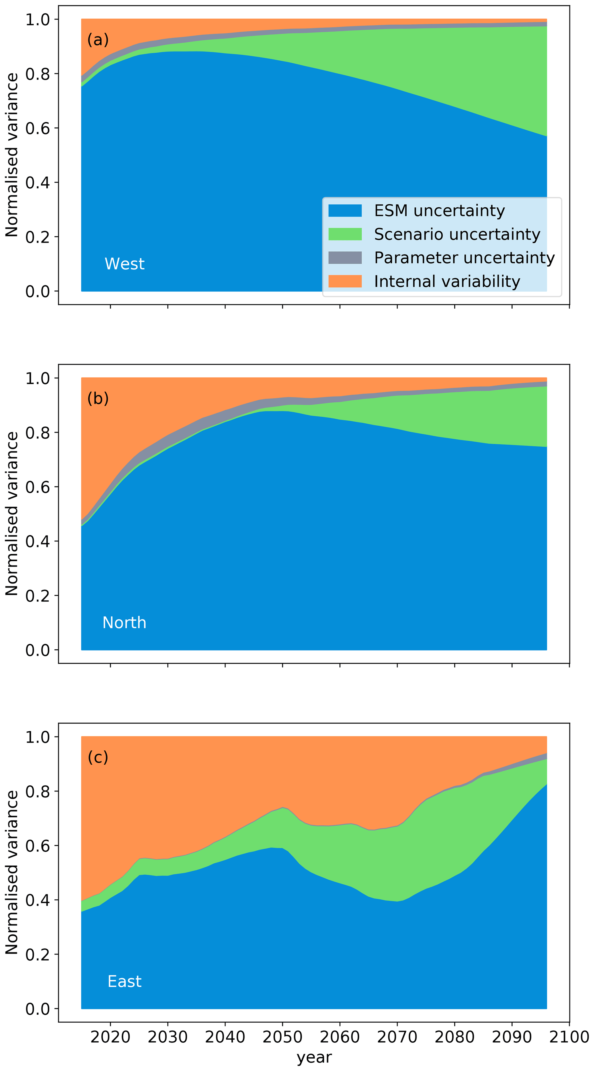
Figure 8Relative variances of the different uncertainty components for three different regions of the GrIS: uncertainty associated with the choice of ESM (blue), uncertainty caused by different emission scenarios (green), uncertainty of different parameter combinations of the snow model (grey), and internal variability (orange), being the variance of the residues of a fourth-degree polynomial fit to the decadal mean integrated SMB. The calculations are described in Appendix C. The time period does not extend to 2100 because the variance splitting approach is applied to the decadal running means of the yearly SMB.
In the western region, the SMB and its different components follow a similar course as for the entire GrIS, except for the amount of SMB decrease per area, which is in the fully transient simulation about 5 times as high (Fig. 7). Additionally, the internal variability is not as important as in the total GrIS, and the scenario uncertainty is slightly higher (Fig. 8a). This shows a high dependence of surface melt on the climate scenario in this region.
In the northern region, the SMB increases with transient precipitation and transient dew point to the same extent (Fig. 7c). Desublimation and sublimation are important contributors to the SMB in this dry region. This is in line with Box and Steffen (2001), who show that 28 % of the accumulation is caused by desublimation at one station in the northeast at 2113 m above sea level. Even the precipitation increase will not dominate in the north by the end of the century. In the fully transient simulation and in the simulation with transient temperature, the SMB decreases strongly and non-linearly at the end of the century (Fig. 7c, orange line). The decrease in SMB is rather late because of the low temperatures in the north at present day. However, when the temperatures rise high enough, ice can be exposed at the surface, which is not always covered by the scarce snowfall and thus triggers a strong albedo feedback. The uncertainty associated with the choice of ESM has a larger share in the north than across all of Greenland because the temperature differences between ESMs are more pronounced, which suggests discrepancies in the simulated sea ice cover. As a consequence, the scenario uncertainty is reduced (Fig. 8b).
In the east, the SMB with transient precipitation follows the SMB with all variables transient closely, showing that the main cause for SMB changes is the precipitation (Fig. 7d). Fettweis et al. (2013) also found increased precipitation in the east because the reduced sea ice cover leads to a moister atmosphere. The uncertainty ranges between ESMs for transient precipitation and the fully transient simulation are also very similar; therefore, the ESM uncertainty is mostly a precipitation uncertainty. The internal variability has a large contribution to uncertainty (Fig. 8c) because the total uncertainty of all other components is small (not shown). The ESM uncertainty is still the largest component, showing an increase at the end of the century (Fig. 8c) when the fully transient SMB stagnates (Fig. 7d).
We simulated the SMB of the GrIS with the snow model BESSI for most of the available climate simulations in the CMIP6 database, using four different climate scenarios and 16 parameter configurations of our snow model. In the high-emission scenario (SSP585), the surface mass loss accelerates and the integrated SMB is about −230 Gt yr−1 at the end of the 21st century, whereas in the low-emission scenario SSP126 the integrated SMB is only slightly lower than in the historical time period and is approximately constant (Table 1, Fig. 2). Taking into account the ice discharge, which amounts to almost 500 Gt yr−1 between 2005 and 2019 (Mankoff et al., 2020), our historical simulations result in a negative total mass balance. Assuming an approximately unchanged discharge, the median SMB in all scenarios implies more substantial mass loss in the future.
The regions with the most pronounced changes in SMB are the west and the north of Greenland. In the west, the SMB is already dominated by melt, and in the north additional melt is not fully compensated by the scarce precipitation. In the east, we simulate a higher SMB than at present day because of a warmer and moister climate in future projections. We find that the choice of ESM has the largest overall influence on the uncertainty in SMB projection, exceeding even the variance between climate scenarios. This effect is localized mostly near the equilibrium line and can be primarily attributed to differences in simulated surface air temperature, followed by differences in the simulated precipitation. Note that we did correct the bias for all ESM simulations based on their performance in the period that overlaps with ERA-Interim (1979–2014) but that no further quality control was performed on the CMIP6 simulations. We speculate that a narrower selection of ESMs, e.g. based on their ability to simulate precipitation patterns and frequencies, could lead to a significant reduction in ESM uncertainty.
The results presented here are in good agreement with previous studies. All ice sheet models in Goelzer et al. (2020) simulated an accelerated mass loss with stronger greenhouse forcing. They used the high-end scenario in CMIP5 with a representative concentration pathway (RCP) that leads to a radiative forcing of 8.5 W m−2 at the end of the 21st century (RCP8.5), comparable to the SSP585 pathway we used here. Detailed SMB estimates are also available from the regional climate model MAR forced by a selection of CMIP6 ESMs (Hanna et al., 2020). This study also finds the familiar acceleration in mass loss. However, four of the five ESMs used to force MAR have an above-average equilibrium climate sensitivity (ECS, Meehl et al., 2020), and thus temperature changes are probably exacerbated. Comparing our simulations with those of MAR that were forced by the same CMIP6 models, we find that in four out of five cases BESSI simulates a higher SMB than MAR (Fig. 9a). This is plausible because BESSI has a stronger bias to higher SMBs than MAR (Fettweis et al., 2020). Notwithstanding this small disagreement, the primary contribution of our study is not the comparison with more complex models, but the fact that the high numerical efficiency of BESSI enables a more comprehensive analysis of model uncertainty, for example by extending the ESM pool to 26. The difference between the highest and lowest SMB in the last simulated years in our ensemble is more than 3 times as large as in Hanna et al. (2020) (Fig. 9a).
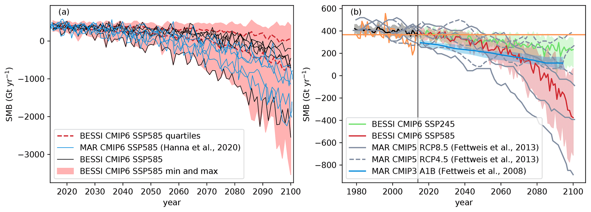
Figure 9(a) SMB simulated by the regional climate model MAR (blue; Hanna et al., 2020, their Fig. 11) and the mean of our simulations (black), forced by the same CMIP6 models, scenario SSP585. The red shading illustrates the minimum and the maximum of SMB for our entire ensemble for this scenario, and the dashed lines are 25 % and 75 % percentiles. (b) Comparison of our simulations with BESSI, Fettweis et al. (2013), their Fig. 4a, and Fettweis et al. (2008), their Fig. 7a. Fettweis et al. (2013) use three different ESMs as input, and thus there are three grey lines for every scenario. The shading are 25 % and 75 % percentiles.
Similar to our high-emission scenario simulations with BESSI, Fettweis et al. (2013) also find a non-linear SMB decrease in simulations with MAR for the high-end scenario of CMIP5 (RCP8.5) (Fig. 9b). Likewise, the roughly linear trend in the MAR simulations forced by the moderate scenario RCP4.5 is qualitatively analogous to scenario SSP245. The differences between ESMs in the SMB simulations of Fettweis et al. (2013) are comparable to the interquartile range of our study. Another moderate scenario simulation with MAR was performed by Fettweis et al. (2008) for the CMIP3 A1B scenario (Fig. 9b), which is an intermediate scenario with greenhouse gas emissions between those in SSP245 and SSP370 (Fettweis et al., 2008; O'Neill et al., 2016). It also shows an approximately linear decrease in SMB but with a smaller uncertainty range than in our moderate SSP245 scenario simulation with BESSI. The multilinear regression performed in Fettweis et al. (2008), which approximates SMB changes as a linear combination of changes in temperature and precipitation, can reduce the uncertainty, as non-linear effects are not included there. Additionally, the smaller variations between ESMs in CMIP3 compared to CMIP6 can have an effect on the uncertainty of the snow model simulations because of the smaller variability in sensitivity to the carbon dioxide forcing (ECS) (Meehl et al., 2020).
The uncertainty in snow model parameters is negligibly small compared to the other uncertainty components, and thus our results hardly depend on the specific set of parameters in BESSI. However, this does not represent the total uncertainty of SMB modelling, as analysed in Fettweis et al. (2020). To address this question fully, our simulations would have to be repeated with every SMB model of that earlier study. This is not practicable because for some of the SMB models the computational requirements are too high to conduct several hundred simulations. Additionally, even RCMs fail in accurately predicting the snowline in years with much melt, leading to substantial biases in SMB prediction because of the albedo difference between snow and ice (Ryan et al., 2019). We expect a larger bias in BESSI because Fettweis et al. (2020) showed that BESSI underestimates the size of the bare ice area and the ablation zone already today. In addition, the total variance of our ensemble is a conservative approximation because our bias correction reduces the variations between the historical simulations of different ESMs and thus also the variability of the climate projections. Furthermore, our assumption of constant topography leads to a bias in SMB projections in 2100 of approximately 10 % (Vizcaino, 2014). Moreover, our simulations neglect the diurnal cycle, which could underestimate refreezing (Krebs-Kanzow et al., 2021). Finally, Greenland blocking leads to increased melt (Hanna et al., 2020), but ESMs do not seem to simulate the blocking correctly (Davini and D’Andrea, 2020). Therefore, our future SMB projections are conservative because the ESMs do not fully represent the expected increase of Greenland blocking in a warming climate. In spite of these caveats, the substantial difference between the ESM and snow model parameter uncertainties suggests that the ESM uncertainty is the largest source of error in the future projections of the GrIS SMB. This key result has two consequences. First, future SMB estimates based on multiple ESMs should explicitly address the quality of the individual simulations in the target region and consider using this skill metric to scale the weight of the individual ensemble members. Second, studies that only include a subset of the plausible climate projections and do not quantify the quality of these selected representations may produce an incomplete picture.
The snow model calculates the SMB for every grid cell on the land surface of Greenland. In the results, only grid cells that belong to the Greenland ice sheet should be considered. The snow model was tuned with the comprehensive RCM RACMO2.3; therefore, the RACMO-ice mask (Noël et al., 2016) is used to identify the grid cells with ice. In addition, we restrict the analysis to grid cells that have an ice thickness of at least 50 m according to the ice sheet topography used in BESSI, which is based on ETOPO1 (1 arcmin resolution) (Amante and Eakins, 2009). The 50 m threshold is chosen to exclude snow caps.
Because we do not simulate ice dynamics, the ice thickness stays constant throughout the simulations with the snow model. For each time step, BESSI calculates the ice that potentially melts at each grid box, regardless of whether ice is actually present or not. The combination of melt of ice, melt of snow, refreezing, snow, rain and runoff is the mass balance. Therefore, grid cells with thin ice cover can distort the mass balance when melt of ice that has already melted is added to the mass balance. This needs to be corrected.
To determine in which grid cells the ice has melted entirely, we subtract the melted ice from the initial ice topography and also consider the inflow by convergence of the lateral steady-state flux. If the result is negative, which means that more ice has melted than would be possible, the grid cell is not considered in the calculation of the mass balance. The ice thickness dh that is added to each grid cell by ice flux is calculated by the advection equation:
where d is the thickness of the ice in the initial topography and dt is the time step. We use the mean ice velocity v from Nagler et al. (2015) and assume that it is constant. Negative values of dh are treated as zero for this correction. In grid cells with thinner ice than a certain threshold, here 50 m, we cannot assume that the ice velocity is constant and therefore we do not take them into account in the SMB calculation.
This simplified calculation of the ice flow results in a lower SMB compared to neglecting the ice flow because it provides ice replenishment that may still melt. The difference amounts to less than 40 Gt yr−1 for all scenarios in the ESM and parameter median averaged over the last 10 years of the simulation. In a fully dynamical ice sheet model, the ice outflow from grid cells would be incorporated, which could cause the ice supply to empty more quickly, leading to a more positive SMB, as empty grid cells are not considered. Presumably, however, the lowering effect of melt–elevation feedback, which is not considered in this study, on the SMB is more substantial. The uncertainty related to the simplified representation of the ice flow is not addressed further.
Several ESMs show strong oversaturation of humidity in areas with very low temperatures, while only small oversaturation occurs in nature due to a lack of freezing nuclei. In ESMs, large oversaturations can be caused by, e.g. interpolation from the ESM levels to near-surface output. Some climate modelling groups truncate the relative humidity to 100 % before they make the data available (Ruosteenoja et al., 2017). To obtain physically realistic values, we truncated the relative humidity to 100 % in all ESMs used in this study. The ESMs HadGEM3-GC31-LL, HadGEM3-GC31-MM, and UKESM1-0-LL have a 360 d calendar, and thus 5 d (spread evenly over the year) are taken twice. We used only one ensemble member of each ESM.
Table B1CMIP6-models (Eyring et al., 2016) used in this project. For each of the listed models, we use the scenarios SSP126, SSP245, SSP370, and SSP585 to force BESSI, except for some missing ESM–scenario combinations. FGOALS-g3 misses SSP126, GFDL-CM4 misses SSP126 and SSP370, GFDL-ESM4 misses SSP245, HadGEM3-GC31-LL misses SSP370, HadGEM3-GC31-MM misses SSP245 and SSP370, and NESM3 misses SSP370. Data were downloaded from https://esgf-node.llnl.gov/search/cmip6/ (last access: 9 December 2021).
To separate the different sources of uncertainty in our projections, we employ the approach of Hawkins and Sutton (2009). Between the different ESMs M, scenarios S, and perturbed snow model parameters in BESSI B, this analysis covers 1952 simulations. The snow model parameters varied in this study are shown in Table C1.
Table C1Parameters in BESSI that are varied in this study. Standard stands for the simulations with only one parameter combination. All parameter combinations use the same albedo routine from Bougamont et al. (2005) and an ice albedo of 0.4.
Assuming that the running average decadal mean of the simulated SMB can be expressed as the result of these uncertainty contributors and time t, as indicated by the subscripts, the snow model output can be divided into a smooth fit with a fourth-degree polynomial and a deviation from that fit:
We analyse the running average decadal means to facilitate the polynomial fit. The polynomial P can be further divided into a constant reference SMB iM that only depends on the ESM, and a deviation :
We perform the analysis with so that we do not have to account for the constant ESM offset. The reference SMB iM is the mean of the annual mean values from the time period 1979–2014, averaged over all BESSI configurations. The spread of the fit matches the spread of the SMB, and the deviations from the fit are only large for few simulations at the end of the simulated period (Fig. C1).
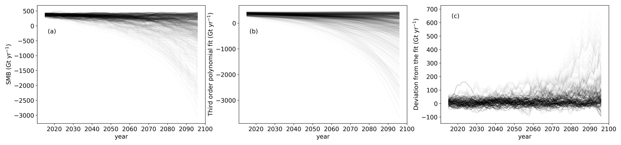
Figure C1(a) Decadal running means of SMB for every parameter–scenario–ESM combination. (b) Fourth-degree polynomial fits of the curves in (a). (c) Deviations of the curves in (a) from the fit in (b).
We give more weight to the ESMs that perform well in the historical period compared to ERA-Interim that we use as a reference. For the calculation of the weights, the average over the SMB of all different parameter combinations for the same ESM is determined first. The absolute deviation of the ESM simulation from ERA-Interim is the difference of the mean SMB over the historical period for all parameter combinations: . Additionally, the performance of the ESMs is also measured by taking the difference in SMB change over the time period between the ESM and ERA-Interim. For every ESM, the total deviation dM is obtained through the Euclidian distance of the absolute deviation and the deviation of the change:
M stands for ESM, E for ERA-Interim, and the numbers for the years. The weights are obtained from the deviation as follows:
The weights are normalized through dividing by their sum, and the normalized weights are denoted WM. The variance of the SMB can be split into components according to the law of total variance. There are six possibilities of how the split is performed exactly.
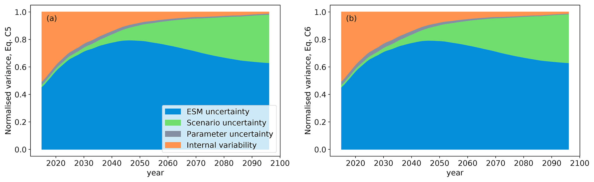
The possibilities (C8), (C9), and (C10) are discarded because expectation values of variances between scenarios are calculated. However, we assume that there should be differences between the scenarios because of their different extents of external forcing. We base our analysis on Eq. (C7), but the results of Eqs. (C5) and (C6) do not deviate much (Figs. 5 and C2).
The internal variability V(t) is the variance of the residues of the polynomial fit. It is considered time dependent because the spread between the different simulations in Fig. C1c changes in time. Therefore, it is calculated for every point in time t over the 20 years around t (t±10a) and over all scenarios and BESSI parameters. The weighted mean of this variance over all ESMs yields the internal variability:
The total variance of the SMB T(t) is the sum of the internal variability and the other uncertainty components that are considered as the ESM uncertainty M(t), scenario uncertainty S(t), and the snow model parameter uncertainty B(t):
For the ESM uncertainty, the weighted variance of the ESMs over the mean parameter configuration is averaged over the scenarios:
For the scenario uncertainty, the variance of the weighted multimodel mean of the mean parameter configuration is taken:
The BESSI uncertainty is the mean uncertainty of all parameters:
The BESSI model code is available on GitHub: BESSI, created by Tobias Zolles, https://github.com/TobiasZo/BESSI/tree/TobiasZo---GSA-model-version (last access: 9 December 2021; Zolles, 2021).
Simulation data of BESSI are available on request. CMIP6 data are available in the CMIP6 database, created by ESGF, https://esgf-node.llnl.gov/search/cmip6/ (last access: 12 September 2021). The surface topography ETOPO1 is available at https://doi.org/10.7289/V5C8276M (Amante and Eakins, 2009). ERA-Interim reanalysis data are available from ECMWF: ERA-Interim, https://www.ecmwf.int/en/forecasts/datasets/reanalysis-datasets/era-interim (last access: 2 July 2019).
KMH prepared the model input, conducted the experiments, analysed the results, and wrote the main part of the manuscript. TZ prepared the model experiments, applied the statistical methods, reviewed the analysis, and revised the manuscript. AB conceived the study, experimental design, and analysis and contributed to the writing of the manuscript.
The contact author has declared that neither they nor their co-authors have any competing interests.
Publisher's note: Copernicus Publications remains neutral with regard to jurisdictional claims in published maps and institutional affiliations.
All authors acknowledge support by the Trond Mohn Foundation. Katharina M. Holube received financial support through an Erasmus+ traineeship. The authors are thankful for the constructive criticism by two anonymous referees.
This research has been supported by the Trond Mohn Foundation (Modeling Englacial Layers and Tracers in Ice Sheets). Katharina M. Holube received financial support through an Erasmus+ traineeship.
This paper was edited by Xavier Fettweis and reviewed by two anonymous referees.
Amante, C. and Eakins, B. W.: ETOPO1 1 Arc-Minute Global Relief Model: Procedures, Data Sources and Analysis, NOAA National Geophysical Data Center [data set], https://doi.org/10.7289/V5C8276M, 2009. a, b, c
Aschwanden, A., Fahnestock, M. A., Truffer, M., Brinkerhoff, D. J., Hock, R., Khroulev, C., Mottram, R., and Khan, S. A.: Contribution of the Greenland Ice Sheet to sea level over the next millennium, Sci. Adv., 5, eeav9396, https://doi.org/10.1126/sciadv.aav9396, 2019. a
Beyer, R., Krapp, M., and Manica, A.: An empirical evaluation of bias correction methods for palaeoclimate simulations, Clim. Past, 16, 1493–1508, https://doi.org/10.5194/cp-16-1493-2020, 2020. a
Born, A., Imhof, M. A., and Stocker, T. F.: An efficient surface energy–mass balance model for snow and ice, The Cryosphere, 13, 1529–1546, https://doi.org/10.5194/tc-13-1529-2019, 2019. a, b, c, d, e
Bougamont, M., Bamber, J. L., and Greuell, W.: A surface mass balance model for the Greenland Ice Sheet, J. Geophys. Res.-Earth, 110, F04018, https://doi.org/10.1029/2005JF000348, 2005. a, b
Box, J. E. and Steffen, K.: Sublimation on the Greenland Ice Sheet from automated weather station observations, J. Geophys. Res.-Atmos., 106, 33965–33981, https://doi.org/10.1029/2001JD900219, 2001. a
Davini, P. and D’Andrea, F.: From CMIP-3 to CMIP-6: Northern Hemisphere atmospheric blocking simulation in present and future climate, J. Climate, 33, 10021–10038, https://doi.org/10.1175/JCLI-D-19-0862.1, 2020. a, b, c
Davy, R. and Outten, S.: The Arctic Surface Climate in CMIP6: Status and Developments since CMIP5, J. Climate, 33, 8047–8068, https://doi.org/10.1175/JCLI-D-19-0990.1, 2020. a
Dee, D. P., Uppala, S. M., Simmons, A. J., Berrisford, P., Poli, P., Kobayashi, S., Andrae, U., Balmaseda, M. A., Balsamo, G., Bauer, P., Bechtold, P., Beljaars, A. C. M., Berg, L. v. d., Bidlot, J., Bormann, N., Delsol, C., Dragani, R., Fuentes, M., Geer, A. J., Haimberger, L., Healy, S. B., Hersbach, H., Hólm, E. V., Isaksen, L., Kållberg, P., Köhler, M., Matricardi, M., McNally, A. P., Monge-Sanz, B. M., Morcrette, J.-J., Park, B.-K., Peubey, C., Rosnay, P. D., Tavolato, C., Thépaut, J.-N., and Vitart, F.: The ERA-Interim reanalysis: configuration and performance of the data assimilation system, Q. J. Roy. Meteor. Soc., 137, 553–597, https://doi.org/10.1002/qj.828, 2011. a
Eyring, V., Bony, S., Meehl, G. A., Senior, C. A., Stevens, B., Stouffer, R. J., and Taylor, K. E.: Overview of the Coupled Model Intercomparison Project Phase 6 (CMIP6) experimental design and organization, Geosci. Model Dev., 9, 1937–1958, https://doi.org/10.5194/gmd-9-1937-2016, 2016. a, b
Fettweis, X., Hanna, E., Gallée, H., Huybrechts, P., and Erpicum, M.: Estimation of the Greenland ice sheet surface mass balance for the 20th and 21st centuries, The Cryosphere, 2, 117–129, https://doi.org/10.5194/tc-2-117-2008, 2008. a, b, c, d, e, f
Fettweis, X., Franco, B., Tedesco, M., van Angelen, J. H., Lenaerts, J. T. M., van den Broeke, M. R., and Gallée, H.: Estimating the Greenland ice sheet surface mass balance contribution to future sea level rise using the regional atmospheric climate model MAR, The Cryosphere, 7, 469–489, https://doi.org/10.5194/tc-7-469-2013, 2013. a, b, c, d, e, f, g
Fettweis, X., Hofer, S., Krebs-Kanzow, U., Amory, C., Aoki, T., Berends, C. J., Born, A., Box, J. E., Delhasse, A., Fujita, K., Gierz, P., Goelzer, H., Hanna, E., Hashimoto, A., Huybrechts, P., Kapsch, M.-L., King, M. D., Kittel, C., Lang, C., Langen, P. L., Lenaerts, J. T. M., Liston, G. E., Lohmann, G., Mernild, S. H., Mikolajewicz, U., Modali, K., Mottram, R. H., Niwano, M., Noël, B., Ryan, J. C., Smith, A., Streffing, J., Tedesco, M., van de Berg, W. J., van den Broeke, M., van de Wal, R. S. W., van Kampenhout, L., Wilton, D., Wouters, B., Ziemen, F., and Zolles, T.: GrSMBMIP: intercomparison of the modelled 1980–2012 surface mass balance over the Greenland Ice Sheet, The Cryosphere, 14, 3935–3958, https://doi.org/10.5194/tc-14-3935-2020, 2020. a, b, c, d, e, f
Franco, B., Fettweis, X., Erpicum, M., and Nicolay, S.: Present and future climates of the Greenland ice sheet according to the IPCC AR4 models, Clim. Dynam., 36, 1897–1918, https://doi.org/10.1007/s00382-010-0779-1, 2011. a
Goelzer, H., Huybrechts, P., Fürst, J. J., Nick, F. M., Andersen, M. L., Edwards, T. L., Fettweis, X., Payne, A. J., and Shannon, S.: Sensitivity of Greenland Ice Sheet Projections to Model Formulations, J. Glaciol., 59, 733–749, https://doi.org/10.3189/2013JoG12J182, 2013. a, b
Goelzer, H., Nowicki, S., Payne, A., Larour, E., Seroussi, H., Lipscomb, W. H., Gregory, J., Abe-Ouchi, A., Shepherd, A., Simon, E., Agosta, C., Alexander, P., Aschwanden, A., Barthel, A., Calov, R., Chambers, C., Choi, Y., Cuzzone, J., Dumas, C., Edwards, T., Felikson, D., Fettweis, X., Golledge, N. R., Greve, R., Humbert, A., Huybrechts, P., Le clec'h, S., Lee, V., Leguy, G., Little, C., Lowry, D. P., Morlighem, M., Nias, I., Quiquet, A., Rückamp, M., Schlegel, N.-J., Slater, D. A., Smith, R. S., Straneo, F., Tarasov, L., van de Wal, R., and van den Broeke, M.: The future sea-level contribution of the Greenland ice sheet: a multi-model ensemble study of ISMIP6, The Cryosphere, 14, 3071–3096, https://doi.org/10.5194/tc-14-3071-2020, 2020. a, b
Graversen, R. G., Drijfhout, S., Hazeleger, W., van de Wal, R., Bintanja, R., and Helsen, M.: Greenland’s contribution to global sea-level rise by the end of the 21st century, Clim. Dynam., 37, 1427–1442, https://doi.org/10.1007/s00382-010-0918-8, 2011. a
Hanna, E., Cappelen, J., Fettweis, X., Mernild, S. H., Mote, T. L., Mottram, R., Steffen, K., Ballinger, T. J., and Hall, R. J.: Greenland surface air temperature changes from 1981 to 2019 and implications for ice-sheet melt and mass-balance change, Int. J. Climatol., 41, E1336–E1352, https://doi.org/10.1002/joc.6771, 2020. a, b, c, d, e, f
Hawkins, E. and Sutton, R.: The Potential to Narrow Uncertainty in Regional Climate Predictions, B. Am. Meteorol. Soc., 90, 1095–1108, https://doi.org/10.1175/2009BAMS2607.1, 2009. a, b, c
Hofer, S., Tedstone, A. J., Fettweis, X., and Bamber, J. L.: Decreasing cloud cover drives the recent mass loss on the Greenland Ice Sheet, Sci. Adv., 3, e1700584, https://doi.org/10.1126/sciadv.1700584, 2017. a
Hofer, S., Lang, C., Amory, C., Kittel, C., Delhasse, A., Tedstone, A., and Fettweis, X.: Greater Greenland Ice Sheet contribution to global sea level rise in CMIP6, Nat. Commun., 11, 6289, https://doi.org/10.1038/s41467-020-20011-8, 2020. a
Knutti, R., Masson, D., and Gettelman, A.: Climate model genealogy: Generation CMIP5 and how we got there, Geophys. Res. Lett., 40, 1194–1199, https://doi.org/10.1002/grl.50256, 2013. a
Krebs-Kanzow, U., Gierz, P., Rodehacke, C. B., Xu, S., Yang, H., and Lohmann, G.: The diurnal Energy Balance Model (dEBM): a convenient surface mass balance solution for ice sheets in Earth system modeling, The Cryosphere, 15, 2295–2313, https://doi.org/10.5194/tc-15-2295-2021, 2021. a
Lehner, F., Deser, C., Maher, N., Marotzke, J., Fischer, E. M., Brunner, L., Knutti, R., and Hawkins, E.: Partitioning climate projection uncertainty with multiple large ensembles and CMIP5/6, Earth Syst. Dynam., 11, 491–508, https://doi.org/10.5194/esd-11-491-2020, 2020. a
Mankoff, K. D., Solgaard, A., Colgan, W., Ahlstrøm, A. P., Khan, S. A., and Fausto, R. S.: Greenland Ice Sheet solid ice discharge from 1986 through March 2020, Earth Syst. Sci. Data, 12, 1367–1383, https://doi.org/10.5194/essd-12-1367-2020, 2020. a
Meehl, G. A., Senior, C. A., Eyring, V., Flato, G., Lamarque, J.-F., Stouffer, R. J., Taylor, K. E., and Schlund, M.: Context for interpreting equilibrium climate sensitivity and transient climate response from the CMIP6 Earth system models, Sci. Adv., 6, eaba1981, https://doi.org/10.1126/sciadv.aba1981, 2020. a, b
Nagler, T., Rott, H., Hetzenecker, M., Wuite, J., and Potin, P.: The Sentinel-1 Mission: New Opportunities for Ice Sheet Observations, Remote Sens., 7, 9371–9389, https://doi.org/10.3390/rs70709371, 2015. a
Noël, B., van de Berg, W. J., Machguth, H., Lhermitte, S., Howat, I., Fettweis, X., and van den Broeke, M. R.: A daily, 1 km resolution data set of downscaled Greenland ice sheet surface mass balance (1958–2015), The Cryosphere, 10, 2361–2377, https://doi.org/10.5194/tc-10-2361-2016, 2016. a, b
O'Neill, B. C., Tebaldi, C., van Vuuren, D. P., Eyring, V., Friedlingstein, P., Hurtt, G., Knutti, R., Kriegler, E., Lamarque, J.-F., Lowe, J., Meehl, G. A., Moss, R., Riahi, K., and Sanderson, B. M.: The Scenario Model Intercomparison Project (ScenarioMIP) for CMIP6, Geosci. Model Dev., 9, 3461–3482, https://doi.org/10.5194/gmd-9-3461-2016, 2016. a, b
Ruosteenoja, K., Jylhä, K., Räisänen, J., and Mäkelä, A.: Surface air relative humidities spuriously exceeding 100 % in CMIP5 model output and their impact on future projections, J. Geophys. Res.-Atmos., 122, 9557–9568, https://doi.org/10.1002/2017JD026909, 2017. a
Ryan, J. C., Smith, L. C., van As, D., Cooley, S. W., Cooper, M. G., Pitcher, L. H., and Hubbard, A.: Greenland Ice Sheet surface melt amplified by snowline migration and bare ice exposure, Sci. Adv., 5, eaav3738, https://doi.org/10.1126/sciadv.aav3738, 2019. a
Sasgen, I., Wouters, B., Gardner, A. S., King, M. D., Tedesco, M., Landerer, F. W., Dahle, C., Save, H., and Fettweis, X.: Return to rapid ice loss in Greenland and record loss in 2019 detected by the GRACE-FO satellites, Commun. Earth Environ., 1, 8, https://doi.org/10.1038/s43247-020-0010-1, 2020. a, b, c
Slater, T., Hogg, A. E., and Mottram, R.: Ice-sheet losses track high-end sea-level rise projections, Nat. Clim. Chang., 10, 879–881, https://doi.org/10.1038/s41558-020-0893-y, 2020. a
Sodemann, H., Schwierz, C., and Wernli, H.: Interannual variability of Greenland winter precipitation sources: Lagrangian moisture diagnostic and North Atlantic Oscillation influence, J. Geophys. Res.-Atmos., 113, D03107, https://doi.org/10.1029/2007JD008503, 2008. a
Vizcaino, M.: Ice sheets as interactive components of Earth System Models: progress and challenges: Ice sheets as interactive components of Earth System Models, WIREs Clim Change, 5, 557–568, https://doi.org/10.1002/wcc.285, 2014. a, b
Yan, Q., Wang, H., Johannessen, O. M., and Zhang, Z.: Greenland ice sheet contribution to future global sea level rise based on CMIP5 models, Adv. Atmos. Sci., 31, 8–16, https://doi.org/10.1007/s00376-013-3002-6, 2014. a
Zolles, T.: BESSI, available at: https://github.com/TobiasZo/BESSI/tree/TobiasZo---GSA-model-version (last access: 9 December 2021), Github [code], 2021. a
Zolles, T. and Born, A.: Sensitivity of the Greenland surface mass and energy balance to uncertainties in key model parameters, The Cryosphere, 15, 2917–2938, https://doi.org/10.5194/tc-15-2917-2021, 2021. a, b, c, d, e, f, g, h, i
Zolles, T. and Born, A.: How does a change in climate variability impact the Greenland ice-sheet surface mass balance?, The Cryosphere Discuss. [preprint], https://doi.org/10.5194/tc-2021-379, in review, 2022. a
Zolles, T., Maussion, F., Galos, S. P., Gurgiser, W., and Nicholson, L.: Robust uncertainty assessment of the spatio-temporal transferability of glacier mass and energy balance models, The Cryosphere, 13, 469–489, https://doi.org/10.5194/tc-13-469-2019, 2019. a, b
- Abstract
- Introduction
- Methods
- Results
- Summary and discussion
- Appendix A: Treatment of melted ice in the snow model results
- Appendix B: Earth system models from CMIP6
- Appendix C: Uncertainty estimation
- Code availability
- Data availability
- Author contributions
- Competing interests
- Disclaimer
- Acknowledgements
- Financial support
- Review statement
- References