High-resolution subglacial topography around Dome Fuji, Antarctica, based on ground-based radar surveys over 30 years

The retrieval of continuous ice core records of more than 1 Myr is an important challenge in palaeo-climatology. For identifying suitable sites for drilling such ice, knowledge of the subglacial topography and englacial layering is crucial. For this purpose, extensive ground-based ice radar surveys were carried out over Dome Fuji in the East Antarctic plateau during the 2017/18 and 2018/19 austral summers by the Japanese Antarctic Research Expedition, on the basis of ground-based radar surveys conducted over the previous ∼ 30 years. High-gain Yagi antennae were used to improve the antenna beam directivity, thereby significantly decreasing hyperbolic features of unfocused along-track diffraction hyperbolae in the echoes from mountainous ice–bedrock interfaces. We combined the new ice thickness data with the previous ground-based data, recorded since the 1980s, to generate an accurate high-spatial-resolution (up to 0.5 km between survey lines) ice thickness map. This map revealed a complex landscape composed of networks of subglacial valleys and highlands. Based on the new map, we examined the roughness of the ice–bed interface, the bed surface slope, the driving stress of ice and the subglacial hydrological condition. These new products and analyses set substantial constraints on identifying possible locations for new drilling. In addition, our map was compared with a few bed maps compiled by earlier independent efforts based on airborne radar data to examine the difference in features between datasets. Our analysis suggests that widely available bed topography products should be validated with in situ observations where possible.

1 Introduction

Long climatic histories, from about 800 ka up to the present, have been studied using deep ice cores drilled at dome summits in the East Antarctic Ice Sheet (EAIS), such as Dome Fuji (Watanabe et al., 2003; Kawamura et al., 2017) and Dome C (EPICA Community Members, 2004). At Dome Fuji Station (77.317^∘ S, 39.703^∘ E; 3810 m a.s.l.), two ice cores were retrieved by the Japanese Antarctic Research Expedition (JARE), extending to 340 and 720 ka, respectively. The second ice-coring project reached a depth of 3035.22 m (Motoyama et al., 2021); the temperature at the ice bottom reached the melting point (Talalay et al., 2020). Detailed information on the basal topography and internal layer structure of the ice sheet is crucial for locating candidate sites for deep drilling. Ground-based ice sheet radar observations were carried out in the Dome Fuji region for prior site surveys from the late 1980s until 2013 (e.g. Maeno et al., 1994, 1995, 1996, 1997; Fujita et al., 1999, 2002, 2003, 2006, 2011, 2012; Matsuoka et al., 2002, 2003). Analyses of JARE data identified subglacial mountains with a thickness of 2000–2400 m centred at approximately 55 km south of Dome Fuji. In addition, these ice thickness data were used in the compilation of the Antarctic ice sheet thickness for BEDMAP (Lythe et al., 2001), Bedmap2 (Fretwell et al., 2013), Alfred Wegener Institute (AWI) gridded data (Karlsson et al., 2018) and BedMachine Antarctica v1 (Morlighem et al., 2020). From the observed features of radio echoes from the ice–bed interfaces, the bed is estimated to be frozen over the mountains with ice thickness of less than ∼ 2500 m (Fujita et al., 2012).

Knowledge gained from ice core studies is crucial for understanding past and present climates and projecting future anthropogenic climate changes. Marine sediment records indicate that the dominant periodicity of the glacial cycles changed from 40 to the current 100 kyr during the mid-Pleistocene transition (0.9–1.2 Ma) (Lisiecki and Raymo, 2005). However, the speed of the mid-Pleistocene transition and the driver of this change in periodicity, particularly the role of atmospheric CO₂ and other greenhouse gases, are not well understood. Antarctic ice cores that exceed 1 Myr should contain essential information about past climate forcing and responses (e.g. Jouzel and Masson-Delmotte, 2010; Fischer et al., 2013; Wolff et al., 2022). However, such continuous ice core records have not yet been identified from polar ice sheets. Accordingly, the International Partnerships in Ice Core Sciences (IPICS) has identified the retrieval of multiple ice cores that extend to 1.5 Ma (termed oldest-ice cores) as one of the most important challenges for ice core studies (Wolff et al., 2020). Numerical modelling studies have suggested that such old ice is likely to exist in the plateau area of the EAIS, where surface accumulation is low, horizontal flow velocities are small, ice is thinner than that at the currently oldest-ice core drilling sites (EPICA Dome C and Dome Fuji), and basal geothermal heat flux is low, which avoids ice stratigraphic disturbance and bottom melting (e.g. Fischer et al., 2013; Van Liefferinge and Pattyn, 2013; Van Liefferinge et al., 2018).

Ice radar observations have been conducted in the vicinity of the domes in the EAIS, such as Dome A (e.g. Bo et al., 2009; Bell et al., 2011), Dome C (e.g. Young et al., 2017; Lilien et al., 2021) and Titan Dome (Beem et al., 2021), which numerical modelling studies have identified as candidate areas for future deep drilling. In the Dome Fuji region, a candidate area for deep drilling, after ground-based radar surveys were conducted by JARE from the late 1980s until 2013, an extensive airborne radar survey was carried out over a 20 000 km² area during the 2014/15 and 2016/17 austral summers (Karlsson et al., 2018) (Fig. S1a). The bed topography map compiled by Karlsson et al. (2018) cannot identify the bedrock undulations of a horizontal scale of less than approximately 10 km due to the spatially sparse (typical survey line spacing of 10 km) observational data and uses interpolation with intense smoothing to fill in blank areas of data. These authors suggested primary areas for potential drilling sites on the subglacial mountains based on the distinction between melted and frozen bottom by ice sheet modelling under the assumption of surface mass balance and geothermal heat flux. Detailed basal topography data with higher spatial resolution are essential to provide further constraints for modelling to improve the site predictions because actual bed topography has much finer scale (i.e. <10 km) mountainous undulations (e.g. Fujita et al., 1999, 2012; Karlsson et al., 2018; Rodriguez-Morales et al., 2020).

New ice-penetrating radar surveys with high spatial resolution and compilation with existing data have been necessary to improve ice thickness maps, which can facilitate the identification of candidate sites for oldest-ice drilling. However, many earlier radar sounding data have shown unfocused along-track diffraction hyperbolae at the ice–bedrock boundary, resulting in potential biases in the estimated ice thickness. The hyperbolic effects mask sharp peaks and steep valleys near such peaks, resulting in underestimation of ice thickness. Focused synthetic-aperture radar (SAR) processing can be used to correct the errors (e.g. Young et al., 2017; Rodriguez-Morales et al., 2020). Another approach is to make the footprint of the radar beam smaller with real-aperture radar soundings. The present study uses real-aperture radar sounders with high-gain Yagi antennae, resulting in improved antenna beam directivity and thus a decrease in hyperbolic features in echoes from the mountainous ice–bedrock interfaces.

To identify suitable drilling sites for very old ice, it is crucial to gain knowledge of the subglacial topography and englacial layering. Here, we present an ice thickness dataset based on ground-based measurements with a high spatial resolution of up to 0.5 km in terms of survey line spacing for the Dome Fuji region. We combined the latest data from ground-based surveys during the 2017/18 and 2018/19 austral summers with earlier data obtained from ground-based surveys carried out by JARE from the 1980s until 2013. We demonstrate how the selection of antennae affects ice thickness assessment in the southern region of Dome Fuji. We constructed new 0.5 km gridded ice thickness data with the same scale as the line spacing (up to 0.5 km) of measurements during the 2017/18 and 2018/19 austral summers. We compare our compilation with a few bed maps compiled by earlier independent efforts, which are mainly composed of airborne radar data, to examine the difference in features between the datasets. Understanding this difference will facilitate the merging of JARE ground-based data and other airborne data in the future. We use the new dataset to examine subglacial conditions to gain further knowledge to identify the presence and distribution of old ice. Finally, we suggest that the candidate area for the deep coring of old ice is much more limited than previously estimated.

2 Study area and methods

2.1 Study area

JARE’s study area around Dome Fuji is situated on the East Antarctic plateau (Fig. 1a). The region shown in Fig. 1b, which covers the southern region of the highest dome summit, is about 12 000 km² and has an elevation range of about 3700 to 3810 m a.s.l. An annual mean air temperature of −54.4 ^∘C was observed at Dome Fuji Station (Kameda et al., 2009). The annual accumulation rate ranges from about 24 mm w.e. a⁻¹ to 10 % below this value (Fujita et al., 2011) (Fig. S2), as estimated from snow stakes and microwave radiometry.

In the 2017/18 austral summer, JARE conducted ground-based radar surveys over a 12 000 km² area with a spacing of 5 km or less. The total length travelled was approximately 2950 km, covering the vicinity of Dome Fuji Station and the southern subglacial mountains (Fig. 1b). Based on the results of these surveys, a more detailed radar survey was conducted on the south side of Dome Fuji in the 2018/19 season as a collaborative research project by the University of Alabama, the University of Kansas, the National Institute of Polar Research (NIPR) and the Norwegian Polar Institute (NPI). Radar data for a total of 2700 km were acquired in a 1000 km² area, covering the subglacial mountain range around the NDF site (77.789^∘ S, 39.053^∘ E; 3763 m a.s.l.). The final spacing between the survey lines was in the range of 0.25–0.5 km. In the present study, we focus on the performance of the incoherent JARE pulse-modulated radar. Ice thickness detected with the wideband radar sounder provided by the Center for Remote Sensing of Ice Sheets (CReSIS), the University of Kansas, is discussed elsewhere (Rodriguez-Morales et al., 2020).

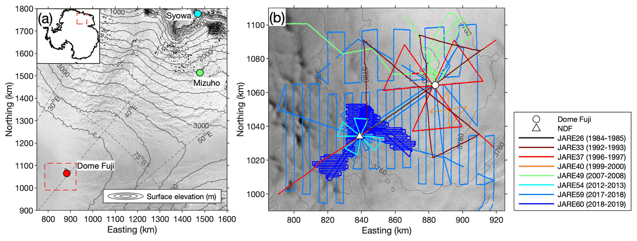
Figure 1 (a) An area of the traverse route between Syowa Station and Dome Fuji in Dronning Maud Land, East Antarctica, with a polar stereographic projection coordinate system. The box indicates the area shown in (b). The inset shows the location of the region in Antarctica. The contours indicate surface elevation with intervals of 200 m (Helm et al., 2014). (b) Dome Fuji region showing the coverage of the JARE radar survey lines. Surface elevation contours have intervals of 20 m. The background is a RADARSAT-1 L1 image (© CSA, 1997).

2.2 Ice radar systems

JARE uses incoherent pulse-modulated VHF radar sounders with a peak transmission power of 1 kW (Table S1). Radar systems with various centre frequencies (179, 60 and 30 MHz and other values) have been used to investigate the mechanisms of radio wave reflection and the frequency dependence of birefringence in the ice sheet in addition to ice thickness measurements (e.g. Maeno et al., 1994, 1995, 1996, 1997; Fujita et al., 1999, 2002, 2003, 2006, 2011, 2012; Matsuoka et al., 2002, 2003). A transmitter pulse width of 60, 250, 500 or 1000 ns was chosen depending on the scientific objectives (measurements of ice thickness or internal layers) and logistics limitations (i.e. antenna size). JARE often chooses a wider pulse for ice thickness measurements to detect the target bed topography with higher-energy electromagnetic waves.

The radar systems were mounted on a snow-tracked vehicle (Ohara Corporation SM100 S-type) (Fig. S3). The transmitting and receiving antennae were attached to either side of the vehicle. The polarization plane of the antennae was arranged either parallel or perpendicularly to the vehicle movement direction.

JARE uses Yagi antennae, and thus the radio waves are linearly polarized, with the polarization plane matching the antenna plane. In the field observations from 1992 to 2013, as shown in the radar survey lines in Fig. S1b, the antennae consisted of one- or two-antenna stacks and three or eight antenna elements per stack (for either transmitting antennae (T_x) or receiving antennae (R_x)), resulting in a total antenna gain (T_x+R_x) that ranges from ca. 15 to ca. 33 dBi. For the two-antenna stacks with eight antenna elements each, the half-power beamwidth was typically ±20 and ±10^∘ for the E and H planes, respectively. For the one-antenna stack with three antenna elements, the half-power beamwidth was typically ±35 for the E and H planes.

The number of antenna stacks and elements determines the antenna gain and directivity. With radar, we need to detect significant echoes from the bed, and thus higher antenna gain allows thicker ice to be detected. In addition, higher directivity is necessary for resolving complex subglacial topography, such as steep mountains, slopes or valley basins. To meet these requirements, for the 2017/18 and 2018/19 field campaigns, we increased the number of antenna stacks and/or elements of the Yagi antennae. In the surveys, the number of antenna stacks was 4, 2 or 1 for either T_x or R_x. The number of antenna elements was 8 to 16 per stack. These settings resulted in an antenna gain (T_x+R_x) of ca. 35 to ca. 27 dBi.

The directivity of the radar beam was also improved by the increase in antenna gain; the half-power beamwidth was typically from ±15 to ±20^∘ for the E plane and from ±5 to ±22^∘ for the H plane. In addition, our radar platform was situated on the ice sheet surface. Thus, the geometry of the wave-spreading effect is expected to be much smaller than that for airborne radar sounding, which typically has a radar height of a few hundred metres above the ice sheet surface. Therefore, the footprint of the radar beam for our ground-based radar platform after 2017 is much narrower than that of our one-antenna stack with three antenna elements used before 2014. Similarly, the footprint of the radar beam for our ground-based radar platform should be narrower than that of the airborne radar antenna with a total antenna gain (T_x+R_x) of about 28 dBi (Nixdorf et al., 1999). The data were recorded on a digital oscilloscope connected to a laptop PC situated inside the tracked vehicle. The three-dimensional coordinates of the radar-sampled points were measured by a global navigation satellite system (GNSS) device attached to the vehicle’s roof, which was almost at the same height as the radar antennae.

2.3 Initial data processing

The ice–bed interface was determined by extracting the peak power of echoes from the bottom of the radargram with semi-automatic detection routines and manual modification. A horizontal smoothing filter was applied to the data using a moving average over 7 s, which corresponds to a horizontal distance of about 20 m at a vehicle speed of 10 km h⁻¹, to increase the signal-to-noise ratio. The ice thickness at the time of observation was converted from the two-way travel time from the surface to the ice–bed interface under the assumption of a propagation velocity of 1.690 × 10⁸ m s⁻¹ determined based on an approximation using the relative permittivity of ice (e.g. Fujita et al., 2000; Saruya et al., 2022b). Here, we estimated this velocity using the relative permittivity value of ice (∼ 3.147 ± 0.010) considering depth-dependent variations in crystal orientation fabrics (Azuma et al., 2000; Saruya et al., 2022a) and temperature within the ice sheet (Motoyama, 2007). Timing errors of the initial trigger in the oscilloscope are possible sources of systematic errors. As an initial step, we calibrated the radar echoes based on a downhole radar target experiment at the Dome Fuji ice-coring site. This calibration inherently included corrections for the thickness of both firn and bubbly ice. We estimated the systematic error in our ice thickness values to be within ±15 m at a thickness of ∼ 3000 m.

The vertical resolution depends on pulse widths; it was 5 and 21 m for our pulse widths of 60 and 250 ns, respectively (Table S1). The bed elevation was obtained from the difference between the GNSS-derived surface elevation and the measured ice thickness. Radar systems used before 2014 had relatively low antenna gains, so the detected bed topography can contain more significant uncertainty than that in the data acquired after 2017. We used the data obtained after 2017 (JARE59 pol179, JARE59 vhf179 and JARE60) as a reference to calibrate the ice thickness obtained from radar measurements before 2014 (JARE33, JARE37, JARE40, JARE49 pol179 and JARE49 vhf60). We considered data within 50 m horizontal distance of each other to be crossover points. We examined the difference in the ice thickness at the nearest points within the area.

A potential bias in the ice thickness was examined for JARE59 and JARE60 data through crossover analysis. For example, JARE59 pol179 data were examined using JARE59 vhf179 and JARE60 data. The ice thickness data showed biases ranging from −37 to 75 m. The ice thickness data acquired from each measurement were corrected for these biases. We subsequently combined the ice thickness point data from each observation into a single dataset.

The combined ice thickness data were interpolated to a 0.5 km resolution grid using an ordinary kriging interpolation method in the open-source geographic information system (GIS) software SAGA GIS (http://www.saga-gis.org, last access: 20 May 2022). The method is based on the experimental variogram with a lag distance of 1 km. The experimental variogram is fitted to a linear model, and the model parameters are determined by minimizing the average squared difference between the observational variogram and the model. We set a search distance of 6 km and a maximum data number of 600, which were determined to be the minimum values required to generate weakly smoothed gridded data over the measured area without data gaps.

2.4 Assessment of uncertainties in ice thickness

We examined the uncertainties in our gridded ice thickness data. The uncertainties were assessed in terms of three error components: (1) the vertical resolution of the radar system, (2) the standard deviations of the ice thickness difference and (3) the standard deviations derived from the kriging interpolation scheme used for generating the gridded data. We estimated the total measurement error at sampled points from components 1 and 2 using the quadratic sum and compiled them into a single dataset. Error component 3, which results from the smoothing of data into sampled points and areas without measurements, was estimated as relative standard deviations. Error component 3 evaluated at individual grids was then converted to absolute standard deviations (in metres) via multiplication by the total error of components 1 and 2.

The uncertainties in the JARE data were also examined by comparing the gridded ice thickness map with measurement points from radar survey lines. The ice thicknesses of the gridded data were interpolated at measurement points using a linear interpolation scheme. The differences in ice thickness were then calculated by subtracting the measurement data from the gridded data.

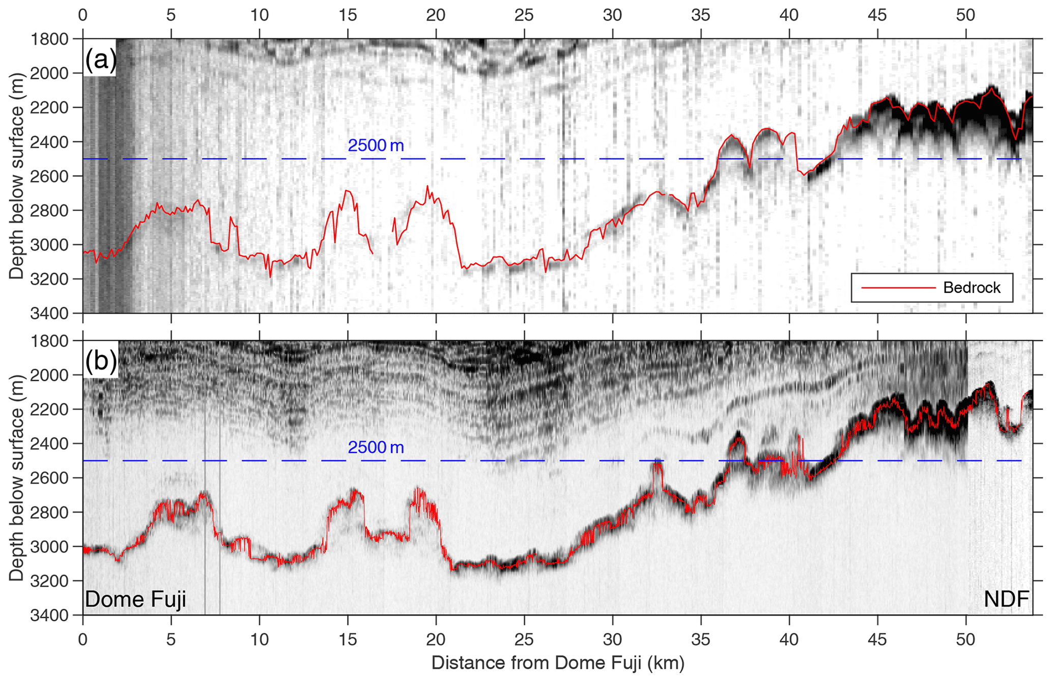
Figure 2 Radargrams between Dome Fuji and NDF acquired by the radar systems used in (a) JARE54 (2012/13) with 3-element Yagi antenna and (b) JARE59 (2017/18) with 11-element Yagi antenna. The lines indicate bedrock topography traced from the radar data. Note that radargrams shown in (b) were generated by data acquired on 17 and 21 December 2017. The colour range in radargrams (a) and (b) is 1.25–1.80 and −110–0 dBm, respectively.

3 Results

3.1 Improvement of ice radar antennae

Figure 2 shows a comparison between radargrams from the radar systems used in JARE54 (2012/13) and JARE59 (2017/18) along the route between Dome Fuji and NDF (Fig. 1b). The radargram acquired from the JARE54 radar has many hyperbolic shapes at the ice–bed interface (Fig. 2a). The electromagnetic waves that reflect the convex terrain mask the electromagnetic wave signals that reflect the valley terrain and slopes, yielding considerable uncertainty when capturing the convex terrain. The radargram acquired from the 11-element Yagi antenna used in JARE59 shows that the hyperbolic effects decreased dramatically (Fig. 2b) where the ice thickness is approximately 2500 m. As imaged by the radargram, the internal ice stratigraphy provides valuable information on the integrity of ice layering and the undisturbed ice column, where coherent scattering appears as layered reflections. The reflection of the layer stratigraphy near the bottom becomes weaker as the ice thickness increases. The continuous horizontal layer from NDF is obscured around Dome Fuji Station, where the ice thickness exceeds 3000 m.

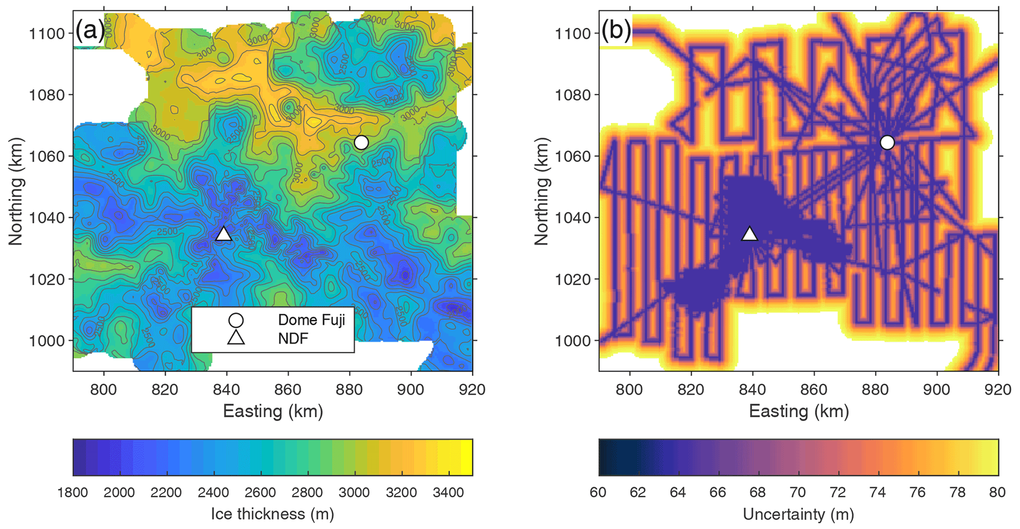
Figure 3 (a) Gridded ice thickness (0.5 km horizontal resolution) and contours with intervals of 100 m. (b) Uncertainty in the gridded ice thickness.

3.2 Ice thickness and bed topography

The gridded ice thicknesses constructed from the compiled JARE radar survey data (hereafter, referred to as JARE data) reveal the presence of a complex landscape around Dome Fuji, with ice thicknesses ranging from 1800 to 3400 m and an average thickness of ∼ 2670 ± 70 m for the investigated area (Fig. 3a). Because the surface topography in the study area is relatively flat (Fig. 1b), the ice thickness closely reflects the bedrock topography. In other words, areas with thick and shallow ice indicate valleys and mountain ranges underlying the ice sheet, respectively. A valley terrain with an ice thickness of 2700–3500 m extends from the north to the west of Dome Fuji, and a bedrock bump with the ice thickness of 2300–2700 m exists further to the northwest. The southern mountains of Dome Fuji consist of complex subglacial ridges and valleys with the ice thickness of 1800–2600 m.

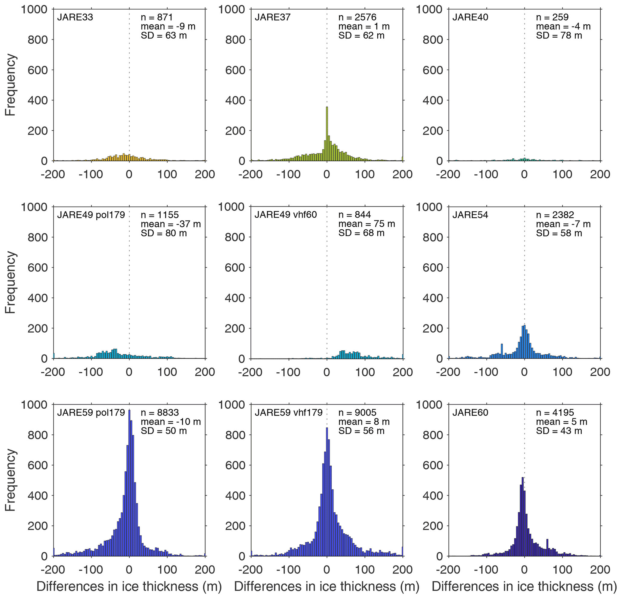
Figure 4 Histogram of the ice thickness difference between the point data from each radar survey and the JARE59 and JARE60 radar surveys. Note that the histograms and statistical values do not account for the geometrical effects of the finite beam pattern of radar antennae on survey data uncertainties.

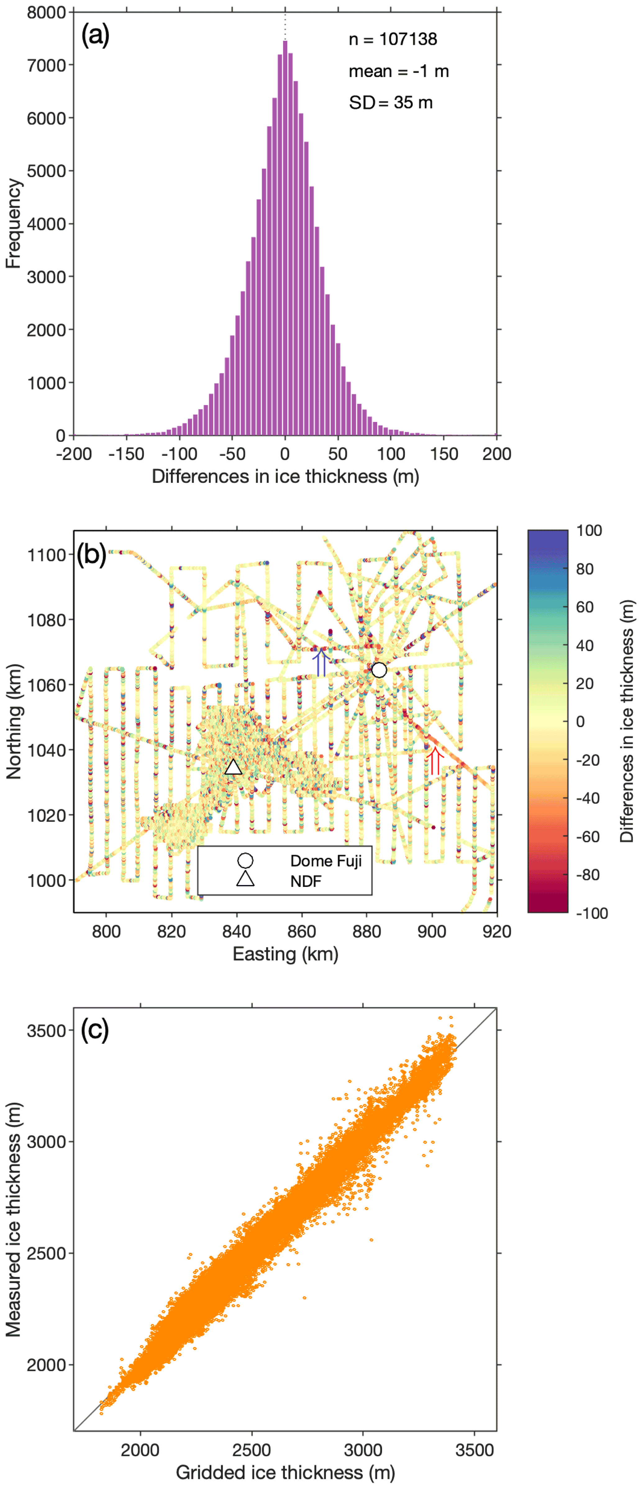
Figure 5 (a) Histogram and (b) spatial distribution showing differences in ice thickness between point measurements and 0.5 km gridded data. Red and blue arrows in (b) indicate the radar lines of JARE37 and JARE49. (c) Scatter plot showing the gridded ice thickness against the point measurement data.

3.3 Uncertainties in ice thickness

The total uncertainty in ice thickness on the interpolated map consists of three factors: two of them are associated with individual measurements, and the third is associated with interpolation. The error components of (1) the vertical resolution of the radar system and (2) the standard deviations of the ice thickness difference were estimated to be 5–85 m (Table S1) and 43–80 m (Fig. 4), respectively. The error component of (3) the standard deviations derived from the kriging interpolation was estimated to be 1 %–34 % (relative standard deviations). Accordingly, the JARE data uncertainties are estimated to be from ±60 to ±80 m with an average of ±71 m (Fig. 3b), which corresponds to within 4 % of the ice thickness in the study area. The uncertainty is typically small near the data points and increases with distance from the data points.

For the 107 138 data points along the radar lines, the mean difference between the interpolated and measured ice thicknesses is less than −1 m, with a standard deviation of 35 m (Fig. 5a). The absolute differences in ice thickness are <50 m for 88 % of the points and >100 m for only <2 % of the points. We do not find clear systematic bias in the gridded ice thickness along radar measurement lines (Fig. 5b). We also examined the overall errors in the ice thickness from gridded data generated by kriging interpolation. A comparison of the gridded data with the measurement data showed an anomaly in ice thickness of <1 % (Fig. 5c), suggesting that the effect of kriging interpolation is constant for all ranges of ice thickness. Note that there is a significant variation in the measurement data relative to the gridded data in the scatter plot because multiple measurement data are compared with the same gridded data in each cell. The gridded ice thickness is >50 m thinner than the measurement data that are situated along the radar lines of JARE37 and JARE49 that run from Dome Fuji to the east and west, respectively (Fig. 5b). The bias along the JARE49 line can be attributable to the bias in the ice thickness in the JARE49 vhf60 measurement data with respect to the JARE59 and JARE60 data, with a mean positive anomaly of 75 m (Fig. 4) (note that the gridded data are corrected for the bias). For the JARE37 line, it is unclear why the gridded data are thinner than the measurement data because there is no appreciable bias in the JARE37 ice thickness with respect to the JARE59 and JARE60 data (Fig. 4).

Quantifying the uncertainty in gridded ice thickness data is complex because it involves multiple variables. However, assessing the uncertainty caused by factors such as the vertical resolution, line spacing of radar observations and interpolation settings of gridded data is essential for resolving the complex subglacial topography in the study area. We suggest that it is necessary to accumulate observation data in the future to assess the optimal uncertainty quantitatively.

4 Discussion

4.1 Improved ice thickness measurements

The use of high-gain and high-directivity antennae resulted in improved accuracy of bedrock topography detection. A crossover analysis of the ice thickness showed that the standard deviations of the ice thickness difference based on data acquired after 2017 (43–56 m) are smaller than those before 2013 (58–80 m) (Fig. 4). Our data suggest that high-gain and high-directivity antennae provide a significant improvement for ice thickness measurement in mountainous terrains. Our 11- and 16-element Yagi antennae had lengths of 5.0 and 5.4 m, respectively, for a frequency of 179 MHz. Even though such vertically long antennae would be difficult to mount on ground-based platforms, they provide an important opportunity for improving incoherent radar systems. Modern coherent radar sounders with phase analysis and SAR processing (e.g. Rodriguez-Morales et al., 2020; Lilien et al., 2021) can remove hyperbolic effects. For improving the accuracy of bedrock topography measurements, we can apply radar with high-gain and high-directivity antennae, state-of-the-art modern radar with focused SAR processing, or both.

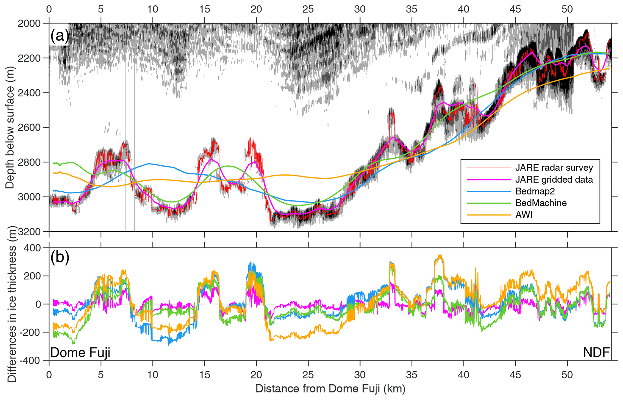
Figure 6 (a) Radargrams based on data collected with the JARE59 radar between Dome Fuji and NDF. The lines indicate bedrock topography traced from the radar data and the JARE, Bedmap2, BedMachine Antarctica and AWI gridded data. (b) Differences in ice thickness of the JARE, Bedmap2, BedMachine Antarctica v1 and AWI gridded data against the JARE radar measurement data. Note that radargrams shown in (a) were generated by data acquired on 17 and 21 December 2017. The colour range in radargrams (a) is −110–0 dBm.

Figure 7 The differences in ice thickness between (a) Bedmap2, (b) BedMachine Antarctica v1 and (c) AWI ice thickness data and the gridded data generated in this study. The bold contours in all plots indicate an ice thickness of 2500 m.

4.2 Comparison with other ice thickness data

We compare our gridded ice thickness with the ice thickness survey data acquired with the JARE59 system to assess the extent to which it reveals the fine undulations of the bedrock topography. We also evaluated the JARE gridded ice thickness with Bedmap2, BedMachine Antarctica v1 and AWI ice thickness along the survey route between Dome Fuji and NDF (Fig. S4). We used a 0.5 km horizontal resolution of BedMachine and AWI data and a 1 km resolution of Bedmap2 resampled to a 0.5 km grid. The ice thickness data acquired by JARE along the route were combined into ice thickness maps to assess the impact of the smoothing effect in the interpolation scheme used for each ice thickness map. Bedmap2, BedMachine and AWI gridded data have compiled ice thickness survey data acquired in JARE33 and JARE37 along the survey route between Dome Fuji and NDF (Fig. S1b). This comparison demonstrates differences in ice thickness between gridded data that contain common point data and that created by different data compilation, smoothing methods and parameter settings. Figure 6a shows that our gridded ice thickness data accurately resolve the undulations in the basal topography with a horizontal scale of >0.5 km. The absolute difference in ice thickness between the gridded and radar-sampled data along the survey line is ∼ 158 m, with an average value and a standard deviation of −6 and 44 m, respectively (Fig. 6b), indicating that our data slightly underestimate the ice thickness on this spatial scale. The most significant differences appear in the sharp peaks at basal topographic highs, where the horizontal scale is smaller than the grid size. The mean differences between the radar measurement points and ice thicknesses from Bedmap2, BedMachine Antarctica and AWI gridded data are 1, −36 and −8 m, with standard deviations of 120, 108 and 148 m, respectively (Fig. 6b). These gridded data are smoother than the radar data and thus tend to overestimate the ice thickness in convex areas of the subglacial terrain and underestimate it in concave areas. For example, BedMachine Antarctica resolves a convex terrain on a horizontal scale of about 5 km at a horizontal distance of 7 and 12 km from Dome Fuji, whereas Bedmap2 and AWI data show a flat terrain (Fig. 6a).

We also examined the differences in ice thickness between the JARE gridded data and the data from Bedmap2, BedMachine Antarctica and AWI over the entire study area. Significant variance was found in all comparisons. The results of a statistical analysis of ice thickness differences are summarized in Table S2. For Bedmap2 and AWI gridded data, the most significant differences appear in the subglacial mountainous terrain south of Dome Fuji (Fig. 7a and c). A comparison revealed overestimation of the ice thickness in the area by ∼ 510 m, resulting from the JARE60 surveys with a fine line spacing (∼ 0.5 km). The ice thickness is underestimated by ∼ 810 m in an area further south of the subglacial mountains, where the subglacial valleys extend from west to east with an ice thickness of >3000 m. The differences in ice thickness are smaller in the vicinity of Dome Fuji Station and further north because Bedmap2 includes JARE data for this area. Although the AWI data also include the JARE measurement data in this area, the ice thickness obtained from AWI data is >200 m thinner northwest of the station. For BedMachine Antarctica data, the differences in ice thickness are smaller than those for the other two datasets (Fig. 7b). Small areas with thicker or thinner ice are distributed in a mosaic pattern. The differences in ice thickness from the three maps relative to the JARE data have small mean values and high standard deviations, suggesting that an interpolation scheme inevitably introduces a significant smoothing effect. Accordingly, our data better delineate the critical features of the subglacial mountain ranges south of Dome Fuji compared with the previously published bedrock topography. The high spatial resolution of the ice thickness data is attributed to the data interpolation smoothing effect being much smaller than that in previous data compilations, which is due to the JARE radar data having a horizontal spacing that is equivalent to the grid size.

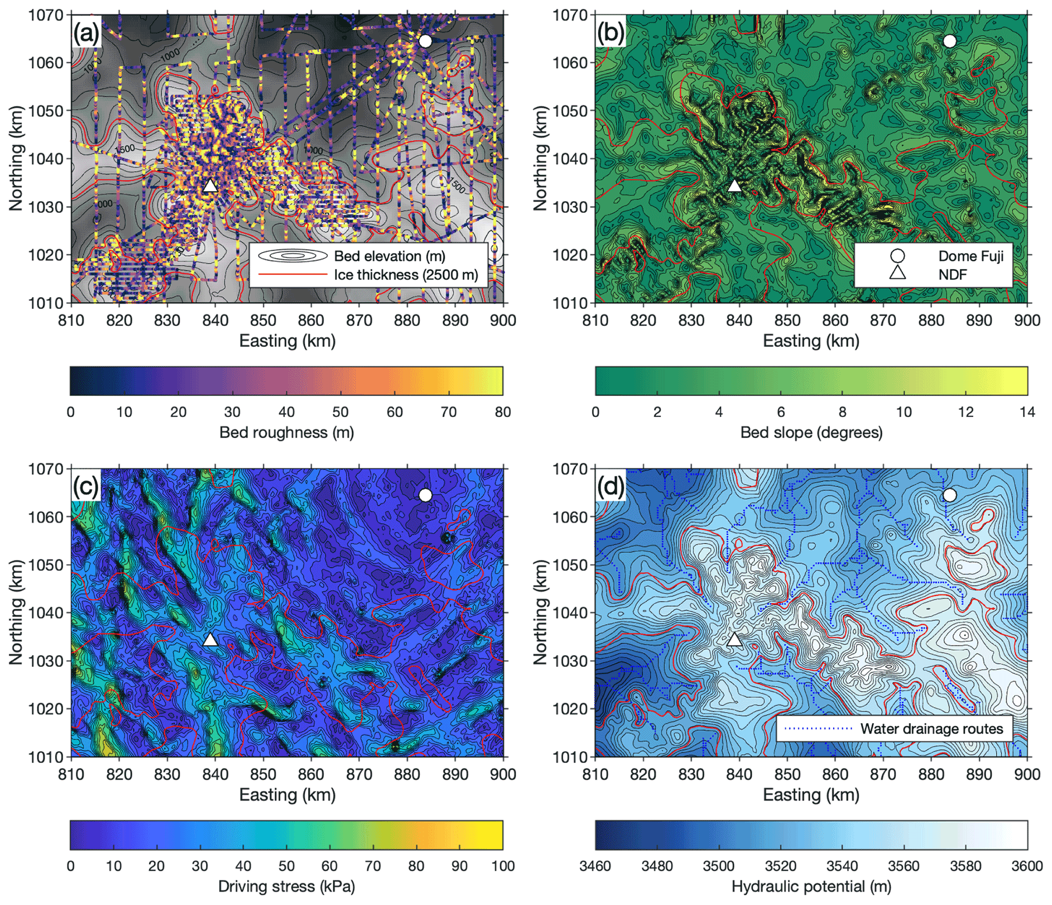
Figure 8 (a) Bed roughness superimposed on new bed elevation data (in greyscale) and (b) the bed slope. Bed elevation contours in (a) have intervals of 100 m. (c) Driving stress using the new ice thickness data and the CryoSat-2 surface DEM (Helm et al., 2014). (d) Hydraulic potential using the new ice thickness and bed elevation data. The estimated drainage routes of the subglacial water are indicated with blue dots. The red contours in all plots indicate an ice thickness of 2500 m.

4.3 Subglacial conditions

To gain further knowledge to identify the optimum drill site, we examined subglacial topographical, glaciological and hydrological conditions with our ice thickness data. Here, we present the roughness of the ice–bed interface, the bed surface slope, the stress state of the ice and the subglacial hydrological condition.

4.3.1 Basal roughness and slope

Bed surface roughness influences the ice to develop a complex deformation pattern in the lowermost part of the ice sheet. The complex deformation field could disturb the stratigraphic continuity of the ice core record. We calculated the bed surface roughness along the ice-radar-surveyed route as the root mean square deviation (RMSD) in detrended bedrock elevation on an 800 m baseline (Shepard et al., 2001; Young et al., 2011, 2017).

The RMSDs at the 800 m length scale typically range from 0–80 m with an average of 26 m in the study area (Fig. 8a). The RMSD obtained in this study is larger than the results by Van Liefferinge et al. (2018)​​​​​​​, who used the AWI compilation ice thickness data (Karlsson et al., 2018), probably due to the spatially dense basal topography data. The RMSD is lower in the summit regions and surrounding subglacial basins of mountain ranges. For example, many of the mountain summits around the NDF, the subglacial basin at 20 km south of the NDF, and a midway region between Dome Fuji and NDF exhibit smoother basal topography. Significantly rougher bedrock surfaces are observed on the slopes, valleys and saddles surrounding the mountain range, where the basal topography is highly variable. Basal surface slope shows a similar spatial pattern to the basal roughness (Fig. 8b). Steep basal surfaces are distributed on the ridges and valleys of the mountain range south of Dome Fuji. Basal topography is relatively flat in the basal trough around Dome Fuji Station. The bed slope ranges from 0–14^∘ with an average of 4^∘ in the study area.

Our results show that the basal roughness is generally high in the subglacial mountainous terrain and lower in the subglacial basins. These spatial patterns are consistent with previously reported in Dome Fuji, Dome A, Ridge B and Dome C in the inland of the EAIS (Bingham and Siegert, 2009; Young et al., 2017; Van Liefferinge et al., 2018). Based on chemical analysis of the lowermost part of the Dome C ice core, Tison et al. (2015) proposed that high basal roughness may change the vertical stress field, changing the thickness of the internal layer in the basal ice. However, the low basal roughness may also be an unfavourable condition for preserving old ice. Eisen et al. (2020) found that in areas in East Antarctica with low flow velocities, such as areas near the inland ice divide, there is a weak spatial relationship in that the bedrock roughness is systematically smaller where the basal conditions are temperate. Indeed, a spatial correlation between smooth basal topography and subglacial lakes has been investigated in the basal temperate area around Dome Fuji (Van Liefferinge et al., 2018). In the Dome Fuji area, the bed is estimated to be temperate at ice thicknesses of more than 2500 m (Fujita et al., 2012), and the presence of subglacial lakes has also been found in these locations (Popov and Masolov, 2007; Karlsson et al., 2018; Van Liefferinge et al., 2018). Even in areas with less than 2500 m of ice thickness, where the bed was estimated to be frozen by Fujita et al. (2012), there is a complex distribution of smooth and undulating basal surfaces (see areas within red contours in Fig. 8a). Further discussion on basal roughness combined with discriminant analysis of basal thermal conditions based on new radar data will be required to narrow down the area where old ice may exist.

4.3.2 Driving stress

Basal ice disturbance is likely to occur when the ice is subjected to horizontal stress due to the surface slope. However, the reduction in horizontal stress may also be due to basal melting, which could eliminate the past climatic record. To examine the influence of the ice stress field on the disturbance of old ice at the base of the ice sheet, we calculated the driving stress from new gridded ice thickness data in conjunction with satellite-derived ice sheet surface elevations. The driving stress τ_d (kPa) is defined as

$$\begin{array}{}\text{(1)}& {\mathit{\tau }}_{\mathrm{d}}={\mathit{\rho }}_{\mathrm{i}}gh\sin \mathit{\alpha },\end{array}$$

where ρ_i is the density of ice (910 kg m⁻³), g is the gravitational acceleration rate (9.8 m s⁻²), h is the ice thickness and α is the slope of the ice sheet surface. Surface slopes were derived from the 1 km resolution CryoSat-2 surface DEM (Helm et al., 2014). The surface slope was then interpolated to a 0.5 km resolution to combine it with the gridded ice thickness data.

Driving stress correlates spatially with surface slope (Figs. 1b and 8c). We observe that driving stress is low around Dome Fuji Station and increases with distance. Basal topography around Dome Fuji Station is less undulating, resulting in less spatial variation in ice thickness. Elevated driving stress was observed over the subglacial mountain ridge around NDF. This high driving stress may disturb the basal ice in these locations. Let us suppose that ice flows over beds with heterogeneous basal topography and resistance. In that case, it will cause undulations on the ice surface, affecting the spatial variation in the surface slope, which affects the local driving stress (e.g. Gudmundsson, 2003; Sergienko et al., 2014). The relationship between undulating basal topography and locally elevated driving stress can be confirmed by the spatial correlation between basal roughness, the basal slope and driving stress. Meanwhile, regions around the subglacial mountain with low driving stress correspond to local subglacial basins. This implies a condition of basal lubrication, and thus melting may have modified the basal ice.

4.3.3 Hydrological conditions

In the Dome Fuji region, the presence of subglacial water, including subglacial lakes and water-saturated sediments, has been identified based on reflected radio echoes from the bedrock surface (e.g. Popov and Masolov, 2007; Fujita et al., 2012; Karlsson et al., 2018). Subglacial water flows from areas of high hydropotential to areas of low hydropotential following the steepest gradient (Shreve, 1972). Hydraulic potential analysis reveals where subglacial water can migrate and provides essential insights into selecting old-ice sites. In the Dome Fuji area, hydraulic potential and the potential subglacial drainage routes have been investigated using airborne radar measurement data (Karlsson et al., 2018). We calculated the hydraulic potential and the potential drainage routes of the subglacial meltwater using new ice thickness data. The hydraulic potential Φ (m) is defined as

$$\begin{array}{}\text{(2)}& \mathrm{\Phi }={\displaystyle \frac{{\mathit{\rho }}_{\mathrm{i}}}{{\mathit{\rho }}_{\mathrm{w}}}}h+z_{\mathrm{b}},\end{array}$$

where ρ_w is the density of water (1000 kg m⁻³) and z_b is the bedrock elevation. The potential water drainage routes were calculated by a multiple-flow-direction algorithm using the topographic analysis software package TopoToolbox developed in MATLAB (Schwanghart and Scherler, 2014). We set an upslope area threshold for defining the subglacial stream network to 100 connected cells (50 km²).

The spatial distribution of hydraulic potential is generally consistent with the basal topography (Fig. 8d). The water flow routing in the hydrological network is initiated over the subglacial mountains. It flows along the valleys to the low subglacial basins, indicating that the geometry of the subglacial hydrological network is dendritic. In the study area, we identified four main drainage systems: flow from the subglacial mountain beneath NDF to the basins located southwest of Dome Fuji (easting of 868 km, northing of 1070 km), west of NDF (825, 1070 km), south of NDF (810, 1025 km) and east of NDF (860, 1010 km). Two of the catchments, west and south of NDF, coincide with locations where subglacial lakes have been identified (Popov and Masolov, 2007; Fujita et al., 2012; Karlsson et al., 2018). Our subglacial hydraulic analysis confirms the features of the basal topography on which subglacial lakes exist (west and south of NDF in Fig. 8d), suggesting that subglacial lakes may be present at two other basins (east of NDF and southwest of Dome Fuji) and other local topographic lows. Basal ice in the subglacial valleys is considered to be melted as drainage streams flow even where the ice thickness is less than 2500 m. Subglacial hydraulic analysis using the new ice thickness data suggested the possible locations of old ice to be at the summits and ridges of subglacial mountains in the southern area of Dome Fuji. Further clarification of the thermal conditions of the ice–bed interface and identification of subglacial lakes is required in this area, using the reflective properties of radar radio signals or ice flow modelling.

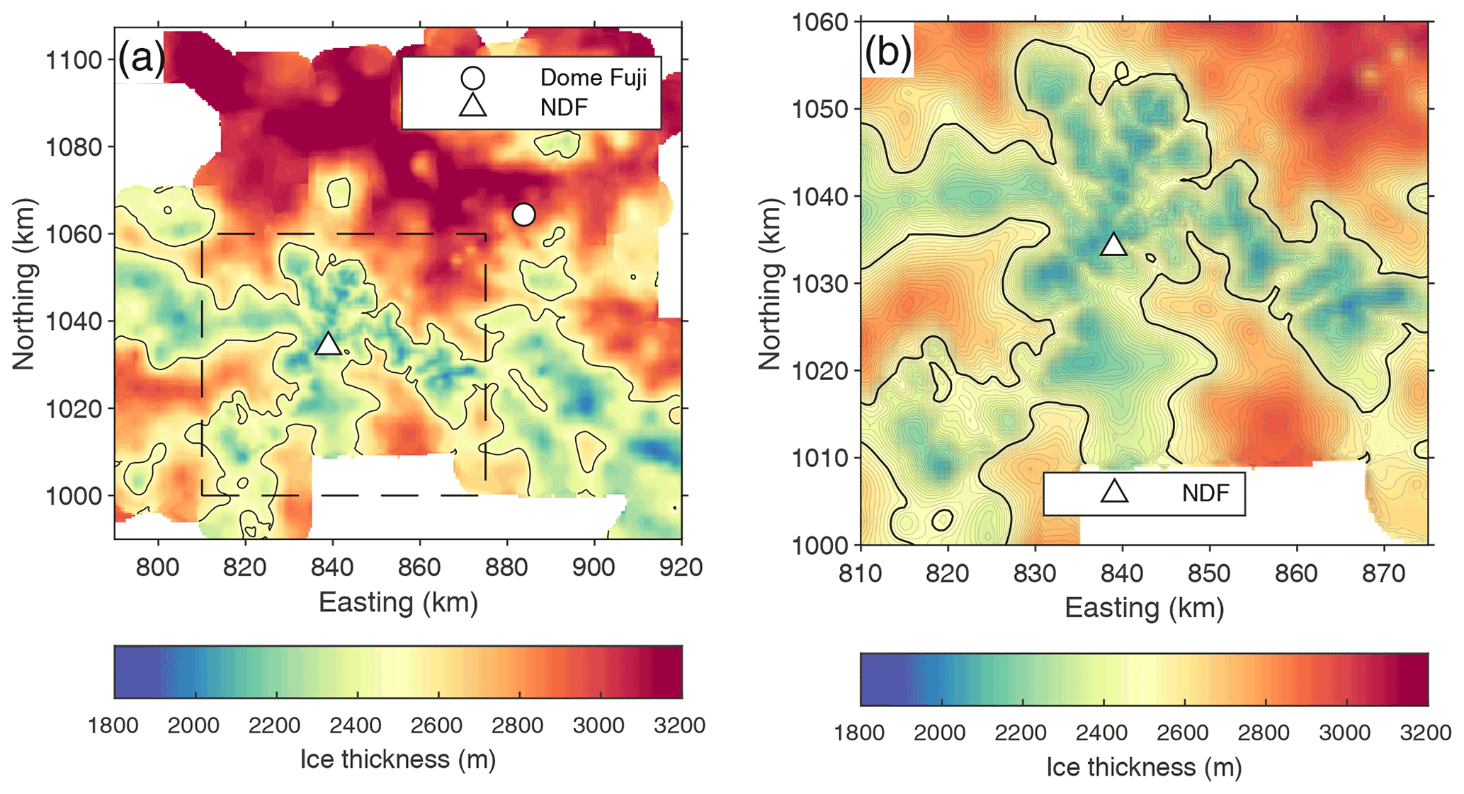
Figure 9 The gridded ice thickness in (a) the study region and (b) the JARE60 observational area. The box in (a) indicates the area shown in (b). The bold contours indicate an ice thickness of 2500 m. The thin contours in (b) indicate ice thickness with intervals of 20 m.

4.4 Prospects for finding the oldest ice around Dome Fuji

The subglacial mountain ranges that extend from the south to southeast of Dome Fuji, where we conducted dense radar measurements, are frozen at the ice–bed interfaces where the ice thickness is approximately <2500 m (Fujita et al., 2012). We could delineate areas with an ice thickness of <2500 m with the JARE data, indicating that a frozen ice-bottom area can be restricted above the ridges and summits of the subglacial mountain range (Fig. 9a). The subglacial terrain exhibits dense dendritic patterns of ridges and summits (Fig. 9b). These areas, where the ice–bed interface should be frozen, appear to be only slightly eroded by ice sheet flow. On the other hand, selective linear erosion occurred in valleys with large ice thickness, suggesting the further erosion of troughs. Fluvial erosion on the East Antarctic continent before 34 Ma, when the ice sheet was formed, is also thought to be a factor in evolving basal troughs (e.g. Jamieson et al., 2005). Note that even in areas with more than 2500 m of ice thickness, old ice may also exist where the ice–bed interface is frozen due to low basal geothermal heat flux and the ice stratigraphy near the base is undisturbed due to low horizontal flow velocity. Regarding the requirements for potential oldest-ice sites, smaller ice thickness is preferred to avoid the possibility of bottom ice melting due to an increase in the insulation effect. In addition to this general view for frozen–melt distinction, our map revealed the presence of complex and steep terrain in the area with reduced errors from hyperbolic effects and high spatial density. This new landscape suggests that finding a potentially suitable drilling site in this area may be more challenging than previously thought.

Even if the bottom of the ice sheet is frozen, the ice sheet is above bedrock ridges, summits, steep slopes or troughs. Finding undisturbed ice layers just above the bed is a prerequisite for oldest-ice drilling. We expect undisturbed ice layers just above the bed to be more likely located above ridges or summits than steep slopes or troughs. Our analyses of driving stresses and hydraulic conditions suggested that the ice over slopes is under high shear stress and that the ice over troughs is subjected to the effects of complex ice flow and bottom melt. Horizontal flow velocity in our study area is <1 m a⁻¹ (see Fig. S7 of Karlsson et al., 2018​​​​​​​), suggesting that basal ice rheology is dominated primarily by vertical normal stress and that horizontal shear stress is relatively small. Under the dominance of the vertical normal stress, horizontal shear appears mainly on subglacial slopes rather than ridges or troughs. Basal troughs are often influenced by basal melt or connected to deeper troughs of more basal melt. Thus, troughs tend to be fast pathways for ice flow. Therefore, we suggest that subglacial ridges in our study area are under simple ice flow conditions, compared to slopes or troughs, to preserve layered conditions.

Low snow accumulation rates are one of the requirements for the presence of old ice in the ice sheet base as they inhibit vertical ice advection and increase the time of existence of the inner layer. The large-scale spatial pattern of the accumulation rate in the Dome Fuji area decreases towards the inland ice sheet (Fig. S2). On the windward (low-latitude) side of an ice divide around Dome Fuji Station, the wind releases precipitation as it slopes up over the ice sheet surface. Then it brings relatively dry air on the leeward (NDF) side due to the orographic effect. For the local scale, previous studies have indicated that the accumulation rate is negatively correlated with the surface slope, and there is also a relationship between the surface and the basal slopes (e.g. Black and Budd, 1964; Furukawa et al., 1996; Fujita et al., 2002, 2011). For example, ground-based shallow ice radar measurements around NDF revealed that the accumulation rate is locally variable at ∼ 30 % and negatively correlated with the surface slope at a length scale of ∼ 2 km (Van Liefferinge et al., 2021). Further analysis between the detailed basal topography revealed by our observations and the accumulation rate will be required to provide new insights into the complex spatially varying surface mass balance distribution, contributing to selecting possible locations for old ice.

Finding suitable locations for very old ice drilling in mountainous areas requires a pinpointing assessment to avoid sites with irregular bed topography. This is the basis as to why we needed the data with a significant decrease in hyperbolic features in the echoes from mountainous ice–bedrock interfaces. After locating possible areas for deep drilling based on the present 0.5 km resolution bed topography, further radar sounding with a higher spatial resolution (i.e. 0.1 km or less) is needed to find the best candidate points in the identified areas.

5 Conclusions

To better understand the detailed bedrock topography for finding potential sites that contain ice that extends to >1 Ma, we conducted ground-based radar measurements with a high spatial resolution across the Dome Fuji region, East Antarctica, in the 2017/18 and 2018/19 austral summer seasons. The antenna performance of the VHF radar systems was greatly improved by high gain and high directivity. We constructed an ice thickness map from the improved radar data and previous data that had been collected since the late 1980s. The differences in ice thicknesses of our gridded data and previously published gridded data were investigated in relation to the radar measurement data to assess the impact of the smoothing effect in the interpolation scheme on the bedrock topography. We also examined the spatial distribution of the ice thickness differences between our data and previous gridded data.

The data acquired using the improved radar systems had a significant decrease in the hyperbolic features at the ice–bedrock interface and allowed basal topography to be identified with higher accuracy. The improved radar systems clearly resolved the internal layer stratigraphy at the lower part of the ice sheet. The new ice thickness data show the bedrock topography, particularly the complex terrain of subglacial valleys and highlands south of Dome Fuji, with substantially higher detail than that in previously published data. The high spatial resolution of the ice thickness data is attributed to the data interpolation smoothing effect being much smaller than that in previous data, which is due to the JARE radar data having a horizontal spacing that is equivalent to the grid size. Our topographic analysis indicates that steep and rough bedrock surfaces extend at the slopes of the basal mountains, while relatively flat surfaces exist at the mountain summit and subglacial basins. Hydraulic analysis implies the presence of subglacial water flow networks and subglacial lakes in subglacial valleys and basins where these were not explicitly detected before. The new ice thickness map and subglacial environment findings set substantial constraints on identifying possible locations for oldest-ice drilling areas. Finally, recognizing the improvement in data quality and comparing existing topographic products, we suggest that widely available bed topography products should be validated with in situ observations where possible.