the Creative Commons Attribution 4.0 License.
the Creative Commons Attribution 4.0 License.
 | 14 Jul 2022
Incorporating InSAR kinematics into rock glacier inventories: insights from 11 regions worldwide
Aldo Bertone
Chloé Barboux
Xavier Bodin
Tobias Bolch
Francesco Brardinoni
Rafael Caduff
Hanne H. Christiansen
Margaret M. Darrow
Reynald Delaloye
Bernd Etzelmüller
Ole Humlum
Christophe Lambiel
Karianne S. Lilleøren
Volkmar Mair
Gabriel Pellegrinon
Line Rouyet
Lucas Ruiz
Tazio Strozzi
Rock glaciers are landforms related to permafrost creep that are sensitive to climate variability and change. Their spatial distribution and kinematic behaviour can be critical for managing water resources and geohazards in periglacial areas. Rock glaciers have been inventoried for decades worldwide, often without assessment of their kinematics. The availability of remote sensing data however makes the inclusion of kinematic information potentially feasible, but requires a common methodology in order to create homogeneous inventories. In this context, the International Permafrost Association (IPA) Action Group on rock glacier inventories and kinematics (2018–2023), with the support of the European Space Agency (ESA) Permafrost Climate Change Initiative (CCI) project, is defining standard guidelines for the inclusion of kinematic information within inventories. Here, we demonstrate the feasibility of applying common rules proposed by the Action Group in 11 regions worldwide. Spaceborne interferometric synthetic aperture radar (InSAR) was used to characterise identifiable moving areas related to rock glaciers, applying a manual and a semi-automated approach. Subsequently, these areas were used to assign kinematic information to rock glaciers in existing or newly compiled inventories. More than 5000 moving areas and more than 3600 rock glaciers were classified according to their kinematics. The method and the preliminary results were analysed. We identified drawbacks related to the intrinsic limitations of InSAR and to various applied strategies regarding the integration of non-moving rock glaciers in some investigated regions. This is the first internationally coordinated work that incorporates kinematic attributes within rock glacier inventories at a global scale. The results show the value of designing standardised inventorying procedures for periglacial geomorphology.
- Article
(14804 KB) - Full-text XML
-
Supplement
(2098 KB) - BibTeX
- EndNote


Rock glaciers are creeping masses of frozen debris in the mountain periglacial landscape. Morphologically, they are characterised by a distinct front, lateral margins, and often by ridge-and-furrow surface topography (Barsch, 1996; Haeberli et al., 2006; Berthling, 2011). These landforms are frequently used as a proxy for permafrost occurrence in cold mountain regions (Haeberli, 1985; Boeckli et al., 2012; Schmid et al., 2015; Marcer et al., 2017; Scotti et al., 2017) and can be important for ice (water) storage estimation (Corte, 1976; Bolch and Marchenko, 2009; Azócar and Brenning, 2010; Jones et al., 2018a), geohazard management (Delaloye et al., 2013; Kummert et al., 2018) and climate reconstruction (Konrad et al., 1999; Kääb et al., 2007, 2021).
The spatial distribution of rock glaciers is generally investigated with the support of geodatabases defined as inventories. Initiatives have risen for decades for inventorying rock glaciers in the main periglacial mountain regions of the world, such as in Asia (e.g. Gorbunov et al., 1998; Schmid et al., 2015; Wang et al., 2017; Jones et al., 2018b; Blöthe et al., 2019; Bolch and Marchenko, 2019; Reinosch et al., 2021), North America (e.g. Liu et al., 2013; Charbonneau and Smith, 2018; Munroe, 2018), South America (e.g. Rangecroft et al., 2014; Falaschi et al., 2015; Barcaza et al., 2017; Villarroel et al., 2018; Zalazar et al., 2020), New Zealand (e.g. Sattler et al., 2016; Lambiel et al., 2019), the European Alps (e.g. Guglielmin and Smiraglia, 1998; Delaloye et al., 2010; Cremonese et al., 2011; Krainer and Ribis, 2012; Seppi et al., 2012; Scotti et al., 2013; Barboux et al., 2015; Colucci et al., 2016; Wagner et al., 2020), the Carpathians (e.g. Necsoiu et al., 2016) and Scandinavia (e.g. Lilleøren and Etzelmüller, 2011; Lilleøren et al., 2013).
In 2018, Jones et al. (2018a) provided an overview of available rock glacier inventories (RoGIs) at a global scale, counting more than 130 inventories worldwide, of which over 90 % were produced after the year 2000. The authors merged all these available inventories to create a global inventory, in order to provide a first-order approximation of volumetric ice content contained within rock glaciers. Their analyses highlighted several limitations on the current inventories, namely the absence of an accessible open-access database, the heterogeneities/variabilities of the existing inventories (due to unequal availability of data sources and on variable local geomorphological skills and institutional support) and the subjectivity in the manual identification of rock glaciers, as also observed by Brardinoni et al. (2019). The authors noted that the main limitation is the absence of a common methodology to provide standardised inventories, making it challenging to create a homogeneous global inventory. Nowadays, the international cooperation of the scientific community represents the key element to solve these open questions.
The International Permafrost Association (IPA) Action Group on Rock Glacier Inventories and Kinematics, launched in 2018 (Delaloye et al., 2018), intends to sustain the establishment of widely accepted baseline concepts and standard guidelines for inventorying rock glaciers in mountain permafrost regions (RGIK – baseline concepts, 2022). For the IPA community, a crucial element to include in standardised RoGIs is the kinematic information. Indirect kinematic information – frequently imprecise because it is related to the operator's interpretations – is often derived from visual observation of morphological (e.g. front slope angle) and vegetation-related indicators (Barsch, 1992; Brardinoni et al., 2019). More precise and accurate approaches based on remote sensing data (e.g. satellite interferometry with Sentinel-1 images; Yague-Martinez et al., 2016) were developed to characterise the rock glacier kinematics at a large scale (Necsoiu et al., 2016; Wang et al., 2017; Villarroel et al., 2018; Strozzi et al., 2020; Brencher et al., 2021). These latter approaches are nevertheless based on different criteria and still lack standardised outputs (Jones et al., 2018a; Brardinoni et al., 2019), essential to integrate kinematic information in standardised RoGIs. In this context, a part of the European Space Agency (ESA) Permafrost Climate Change Initiative (Permafrost_CCI) project so-called CCN2 (https://climate.esa.int/en/projects/permafrost/; last access: 10 October 2021) – following the baseline concepts proposed by the IPA Action Group (RGIK – baseline concepts, 2022; RGIK – kinematic, 2022) – developed specific guidelines (RGIK – kinematic approach, 2020) to systematically integrate kinematic information within RoGIs, exploiting spaceborne interferometric synthetic aperture radar (InSAR) data. The guidelines define common rules, intended to reduce subjectivity, which is a potential source of uncertainty and variability. To summarise the workflow, moving areas (MAs) identified with actual movements are first delineated and characterised in terms of velocity class based on interferometric data. The inventoried MAs are then used to assign kinematic information to rock glaciers. Existing RoGIs or newly compiled inventories are exploited to circumscribe the identification of MAs.
In this work, we present the guidelines developed within the ESA Permafrost_CCI project in collaboration with the IPA Action Group (RGIK – kinematic approach, 2020). Our main aim is to explore and demonstrate the feasibility of an international joint effort to include kinematic information in RoGIs. To achieve this goal, we apply the aforementioned guidelines in 11 regions of the world. Most existing inventories do not include kinematic information (Jones et al., 2018a). Here, we are the first to consistently derive semi-quantitative standardised kinematic information on rock glaciers in many regions around the globe. This paper includes the description of the guidelines, a collection of results and general considerations based on the observations. A product validation is also conducted with independent measurements in some specific cases. As this paper is the result of a large cooperative work and builds on recently published guidelines, it does not present definitive results and conclusions. At this stage we are not concerned with the exhaustive interpretation and comparison of the 11 investigated RoGIs. We focus here on discussing the advantages, limitations and potential of the proposed standardised approach to support the integration of kinematic information in inventories at a global scale.
We investigate 11 periglacial regions with various environmental parameters distributed around the world (Fig. 1, Table 1), covering eight major mountain ranges over five continents. Their spatial extent ranges from 250 to 7200 km2 (Table 1), with an approximate median of 1600 km2. All study areas have permafrost conditions, but in some places only in the higher parts of the landscape.
Three study sites are located in the European Alps: western Swiss Alps (Switzerland), southern Vinschgau/Venosta Valley (Italy) and Vanoise Massif (France). Five study sites are located in the sub-Arctic to high Arctic regions: Troms and Finnmark (northern Norway), Nordenskiöld Land (Svalbard), Disko Island (Greenland) and Brooks Range (Alaska, USA). One site is in Central Asia: northern Tien Shan (Kazakhstan). One site is in South America: Central Andes (Argentina). One site is in Oceania: central Southern Alps (New Zealand).
In Nordenskiöld Land (Svalbard), an entirely new RoGI is generated. For the remaining 10 regions, existing inventories or partial inventories were available. Detailed information on the geographical parameters of these investigated regions and references to the available RoGIs are presented in Table 1. Additional information for each region is included in Supplement Sect. A “Description of study areas”.
Table 1Descriptions of geographic settings, RoGI references and InSAR data used for each investigated region.
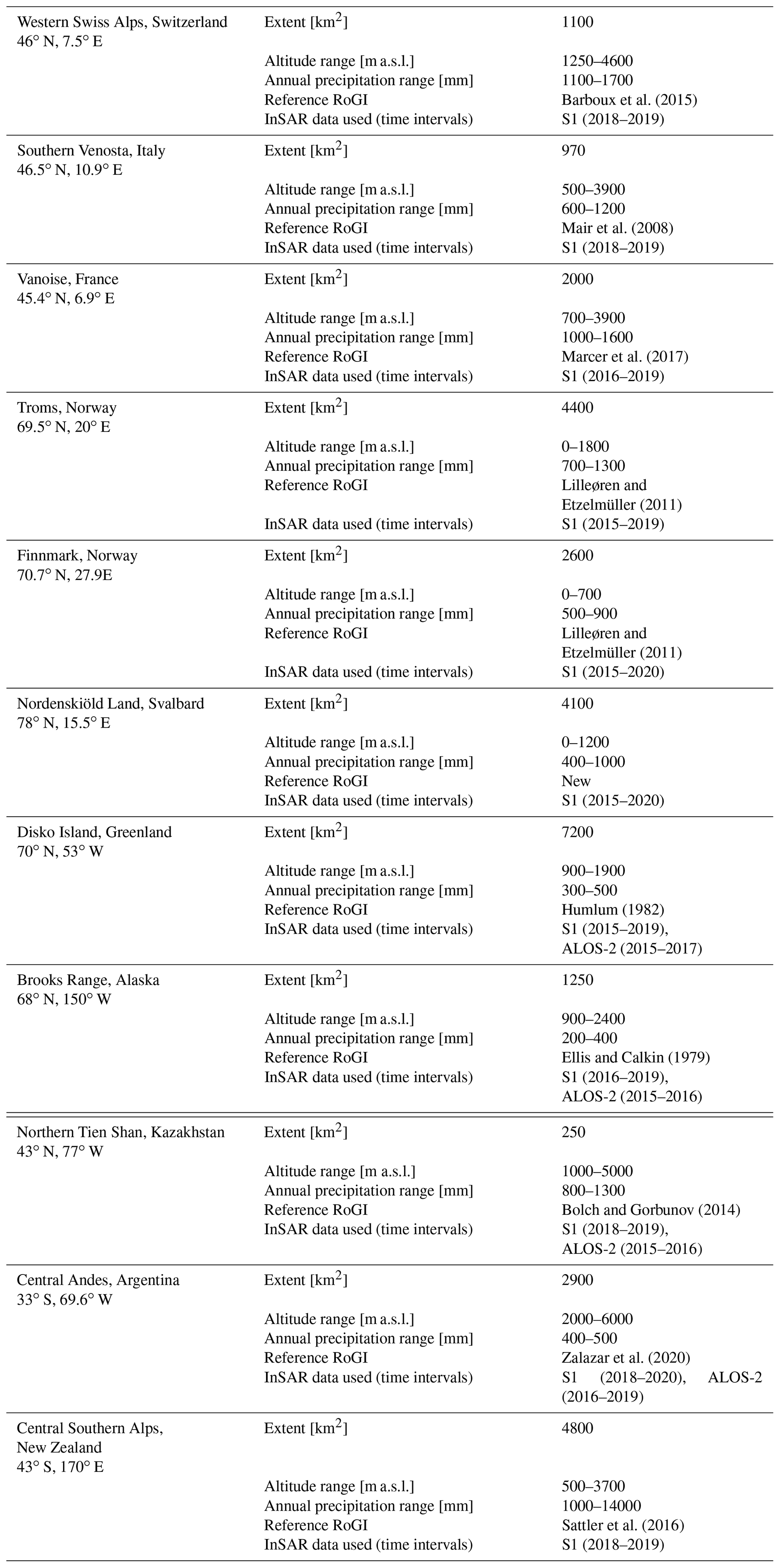
Synthetic aperture radar (SAR) data from the Sentinel-1 (S1) and ALOS-2 satellites used in the present work (Table 1) are collected in both SAR geometries (i.e. ascending and descending) to ensure the best line-of-sight (LOS) orientation (Liu et al., 2013; Barboux et al., 2014). As snow cover is a severe limitation for InSAR (Klees and Massonnet, 1998), only snow-free periods are considered (from July to September and from January to March for the Northern Hemisphere and Southern Hemisphere, respectively). Residual snow periods are detected by identifying extended interferometric decorrelation on InSAR data (e.g. Touzi et al., 1999). Sentinel-1 images are acquired in interferometric wide swath mode with a 250 km swath at 5 m (range) by 20 m (azimuth) spatial resolution. ALOS-2 images are collected in fine mode with a swath width of 70 km and spatial resolution of about 10 m (both range and azimuth). The information on the satellite data used and the time intervals considered for the investigated regions are presented in Table 1.
Depending on availability in each region, additional data such as aerial orthoimages, digital terrain models (DTMs) and DTM-derived products (e.g. hillshade) are included. The complete list of data used for each investigated region is included in Supplement Sect. A “Description of study areas”. Additional kinematic measurements from differential global navigation satellite system (DGNSS) available for 17 rock glaciers in the western Swiss Alps (Delaloye and Staub, 2016; Kummert and Delaloye, 2018; PERMOS, 2019; Strozzi et al., 2020), Vanoise (Marcer et al., 2020), Nordenskiöld Land (Matsuoka et al., 2019), Central Andes (Blöthe et al., 2021), central Southern Alps regions and for four frozen debris lobes (FDLs) in the Brooks Range (Darrow et al., 2016) are used for qualitative validations. For the purposes of this study, measurements of FDLs are not differentiated from rock glaciers for the Brooks Range study area. Feature tracking measurements on optical aerial photographs are also available for nine rock glaciers in the Troms (Eriksen et al., 2018), Nordenskiöld Land and northern Tien Shan (Bolch and Strel, 2018; Kääb et al., 2021) regions.
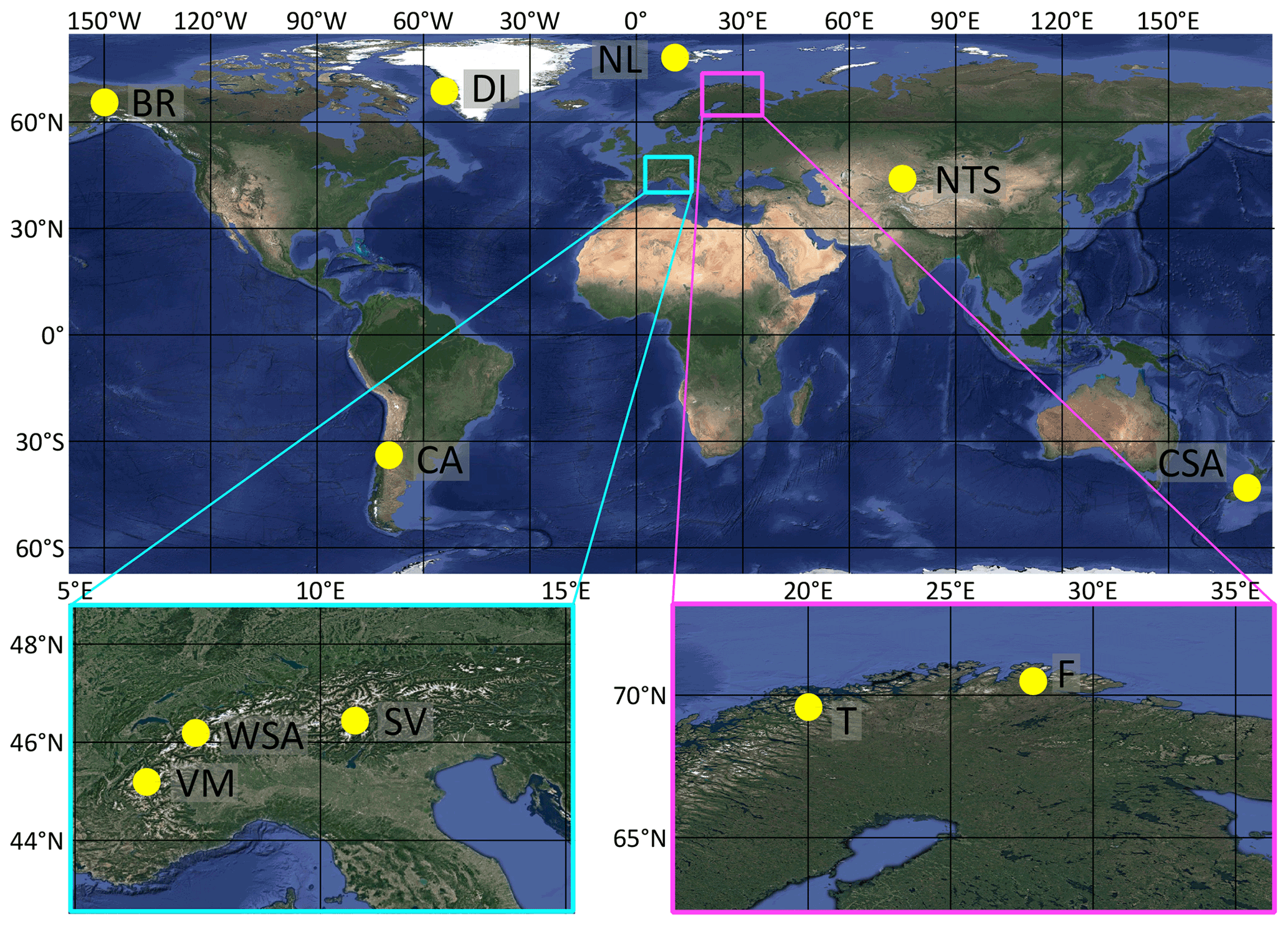
Figure 1Location of the 11 investigated regions (yellow dots): Nordenskiöld Land (NL), Disko Island (DI), Brooks Range (BR), northern Tien Shan (NTS), Central Andes (CA) and central Southern Alps (CSA). The western Swiss Alps (WSA), southern Venosta (SV), Vanoise Massif (VM), Troms (T) and Finnmark (F) are visible in two enlarged panels. Orthoimages from © Google Earth 2019.
3.1 Workflow and input data
The technical aspects related to rock glaciers and presented below are contained in the documents of the IPA Action Group (RGIK – baseline concepts, 2022; RGIK – kinematic, 2022). These documents are constantly discussed and updated by the scientific community and are therefore susceptible to changes, evolutions and improvements. This work is in accordance with the versions produced in March and May 2022. A RoGI consists of a geodatabase, containing the rock glaciers' locations as points and additional information such as activity rates and geomorphological parameters. Optional information, such as the geomorphological delineations with polygons, can be included. Hereafter, the abbreviation RoG is used to refer to a rock glacier unit, defined as a single lobate structure that can be unambiguously discerned according to morphologic evidence such as frontal slope, lateral margins, and ridge-and-furrow topography (RGIK – baseline concepts, 2022). The spatial connection from other (adjacent or overlapping) units can be determined by distinguishing different generations of landforms (e.g. overlapping lobes), different connections to the upslope unit or specific activity rates. A rock glacier “unit” is differentiated from a rock glacier “system” (i.e. a landform identified as a rock glacier), which is composed of either one single or multiple rock glacier units that are spatially connected either in a toposequence or in coalescence. Because of practical and technical limitations, the minimum size of a considered RoG is about 0.01 km2.
The systematic procedure contained in the guidelines (RGIK – kinematic approach, 2020) follows the baseline concepts (RGIK – baseline concepts, 2022; RGIK – kinematic, 2022) and consists of three phases described below and illustrated in Fig. 2. The aim of this procedure is to implement the kinematic information in the inventories, especially for the RoGs affected by movement, to reduce the subjectivity of operators' interpretations and thus have a more accurate and standardised classification.
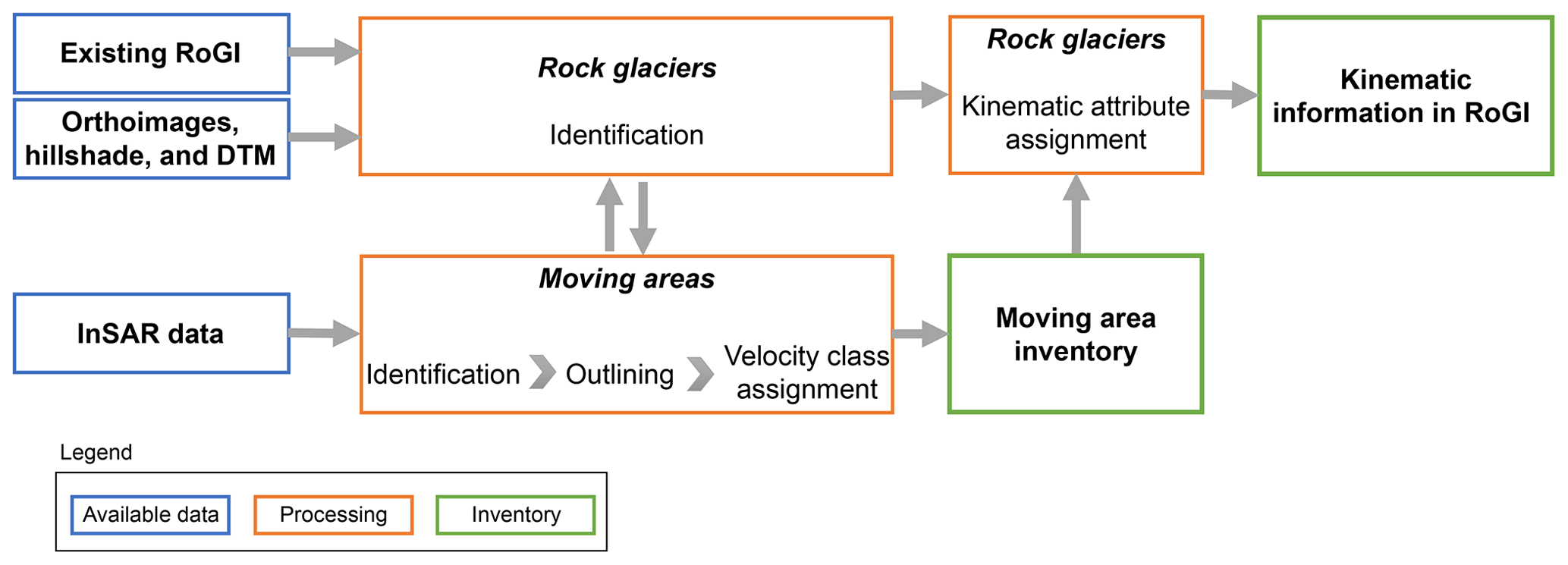
Figure 2Conceptual diagram of the standardised method for producing a moving-area inventory and a RoGI that includes kinematic information. The analysis is performed in a GIS environment.
The first phase consists of the identification of RoGs. For this purpose, existing RoGIs or other forms of information such as from the literature are used. When inventories are not available over the investigated region (e.g. Nordenskiöld Land), the landform identification is performed following the baseline concepts proposed by the IPA Action Group (RGIK – baseline concepts, 2022); systematic visual analysis of the landscape with satellite or airborne optical images (orthoimages and DTM-derived products), field visiting or supervised/unsupervised methods that allow a systematic identification of RoGs can be used (Marcer, 2020; Robson et al., 2020). Within this work, the identified RoGs are distinguished using manually positioned dots on each landform, able to discriminate each RoG clearly without ambiguity (e.g. in the centre of the lobe of the RoG). This initial phase is very important, because the greater the completeness of the RoGs identified, the greater the completeness of the products obtained in the following two phases.
The second phase consists of identifying, outlining and assigning velocity classes to MA – i.e. areas identified as having slope movement with InSAR data – related to the previously identified RoGs. MAs are included within inventories using polygons. This phase is conducted in parallel with the RoG identification, because additional landforms potentially missed can be identified when characterised by MAs through an iterative process between the identifications of MAs and RoGs.
The third phase consists of assigning kinematic attributes to RoGs by exploiting the velocity classes and extents of the MAs that cover the RoGs. This information is then implemented within the inventory. Thus, a kinematic attribute represents the overall movement rate of a RoG, while the MAs document the detailed velocity distribution within the RoG.
In this work, further phases of semi-quantitative assessments are conducted on specific RoGs to verify the correctly assigned kinematic categories, comparing the MA velocity classes and the RoG kinematic attributes with independent measurements acquired during the same time frame. An additional effort adopted to further reduce the subjectivity, misclassifications and errors and increase the overall reliability of the products consists of multiple phases of correction and adjustment conducted by a second operator. The results produced by the first operator are checked by a second operator. In order to optimise the work, operators with both InSAR and geomorphological backgrounds are involved, and study areas already known by the operators are considered to make the best use of the operators' knowledge.
Below in Sect. 3.2 we introduce the basic principles of InSAR. Subsequently in Sect. 3.3 we describe the details of the InSAR methods used to produce the moving-area inventories. The procedure to assign a kinematic attribute to a RoG is described in Sect. 3.4. More details are further described in the practical guidelines (RGIK – kinematic approach, 2020) and in Tables S1 and S2 in the Supplement.
3.2 Basic principles of interferometric synthetic aperture radar (InSAR)
InSAR is a powerful and consolidated technique to detect and map ground movement at the regional scale (Klees and Massonnet, 1998; Massonnet and Feigl, 1998). Systematic acquisitions and wide spatial coverage of the new generation of satellites such as Sentinel-1 make InSAR the most suitable tool for the global mapping objectives of this work (Yague-Martinez et al., 2016).
InSAR processing consists of computing the interferometric phase differences (i.e. the interferograms) from pairs of images with different time intervals (from a few days up to annual) (Massonnet and Souyris, 2008; Yague-Martinez et al., 2016). After geometric, topographic and atmospheric corrections, interferograms provide quantitative measurements of the superficial movements (Klees and Massonnet, 1998; Yague-Martinez et al., 2016).
Despite the potential of InSAR, some limitations apply. First, InSAR provides the observation of the 3D surface deformation component projected along the radar look direction (i.e. the line of sight, LOS), and the measurement is not sensitive to displacements oriented perpendicular to the LOS orientation (Liu et al., 2013; Barboux et al., 2014; Strozzi et al., 2020). Therefore, displacements towards north or south are more affected by geometric distortions, and the magnitude of the displacements might be largely underestimated (Klees and Massonnet, 1998; Liu et al., 2013). Second, steep terrain is masked by geometric distortions known as layover and shadow in mountainous areas (Klees and Massonnet, 1998; Barboux et al., 2014). To reduce the above limitations, both ascending and descending geometries are used in this work, allowing the selection of the best geometry according to the orientation of each RoG (Barboux et al., 2014; Strozzi et al., 2020). Third, the rate of terrain movement that can be detected depends on the time interval of the interferogram, the spatial resolution and the wavelength of the satellite (Massonnet and Feigl, 1998; Barboux et al., 2014; Villarroel et al., 2018; Strozzi et al., 2020). Lastly, artefacts due to uncompensated for atmospheric delays (Yu et al., 2018) and decorrelation or phase bias due to changes in physical properties of the surface (e.g. vegetation, snow, soil moisture; Klees and Massonnet, 1998; Zwieback et al., 2016) can mask the displacement measurements. To reduce these limitations, it is important to rely on a slack of several interferograms from different time periods.
3.3 Moving-area inventory with InSAR
A MA is defined in the guidelines as an area at the surface of a RoG in which the observed flow field (direction and velocity) is uniform (spatially consistent and homogenous). The MA represents the movement rate of the RoG or part of it, detected along the one-dimensional LOS. Each MA is related to (i) a specific “observation time window” (e.g. summer or annual) during which the movement is measured and to (ii) a specific “temporal frame” (year(s)) during which the periodic measurements are repeated and aggregated. The minimal observation time window is 1 month during snow-free periods, detected within a temporal frame of at least 2 years. These time intervals are intended to average possible short, seasonal and multi-annual variations in the dynamics of RoGs (Wirz et al., 2016; Kellerer-Pirklbauer et al., 2018) that can distort the measurements. Observation time windows and temporal frames are documented in the produced moving-area inventories.
MAs are identified and outlined by means of polygons, when the signal of movement is detectable on InSAR data. A MA does not necessarily fit the geomorphological outline of the RoG (Fig. 3). For instance, a MA can override the geomorphological limits of a RoG, several polygons of MAs can be related to the same landform and a slower MA that incorporates one or more faster areas can exist (Fig. 3).
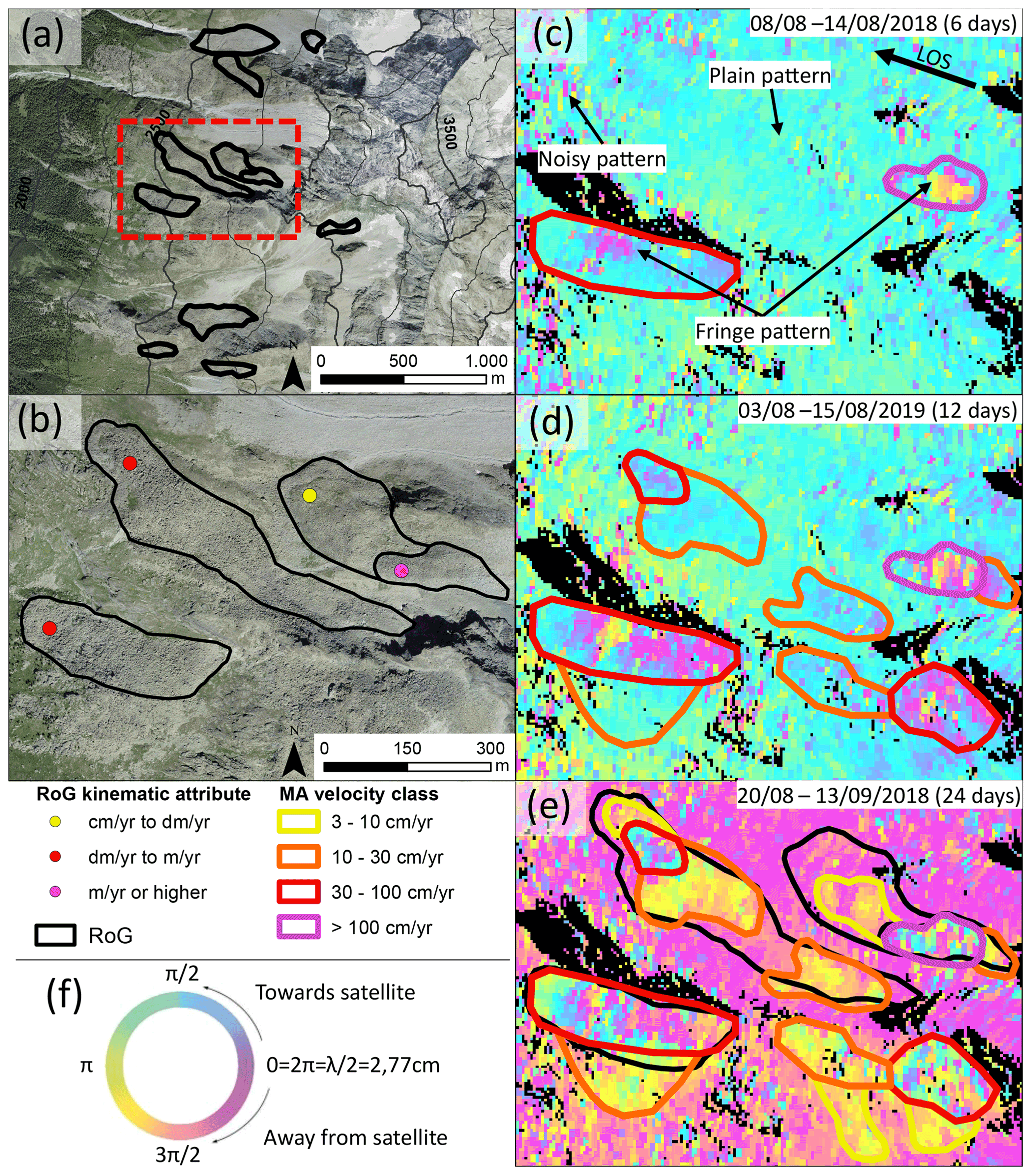
Figure 3Example of a RoGI in the Arolla region (location: N, E, 2750 m a.s.l.), Swiss Alps (a); outlines of RoG are in black, and the location of an investigated area (a) is in red. Orthoimages from © Google Earth 2019. (c–e) Sentinel-1 interferograms from the descending orbit, including examples of InSAR signal patterns; layover and shadow areas are masked out (black). Two MAs are detected on the 6 d interferogram (c). Using 12 and 24 d, additional MAs are visible (d, e). This is an example where the MA outlines do not fully match the geomorphological outline of the RoGs. MAs (SE-border) not related to RoG are visible and mapped. Based on MAs, the kinematic attributes are assigned to RoGs (b). Fringe cycle related to the change of colour (f); a complete fringe cycle is equivalent to a change of half a wavelength (2.77 cm for Sentinel-1) in the LOS direction.
Standardised velocity classes are assigned to each MA. They are meant to (i) facilitate the subsequent assignment of kinematic attributes to the RoGs and (ii) reduce the error and the degree of operator's subjectivity in assigning a specific velocity. A small number of defined classes reduces the variability in choosing one class over another, despite generating a loss of information (i.e. precise velocities) and creating biased information when the velocities are close to the class boundaries. As the guidelines are intended to obtain as standardised of results as possible, six main velocity classes are chosen to balance the above rationale. Following recent studies (e.g. Barboux et al., 2014), the velocity classes, listed in order of increasing velocity, include “< 1”, “1–3”, “3–10”, “10–30”, “30–100”, and “> 100 cm yr−1”. Two additional classes include “Undefined” when velocity cannot be reliably assessed and “Other” when a more accurate velocity can be assigned. The boundaries between the classes are selected taking into account the investigative capabilities of the InSAR, as interferograms with shorter time intervals allow for detection of high velocities, while interferograms with longer time intervals detect lower velocities. For this reason, the velocity classes are related to the time intervals at which movements are detected by a coherent signal. For example, following Barboux et al. (2014), a coherent signal visible on annual Sentinel-1 interferograms allows for documenting velocities ranging from 0.2 to 3 cm yr−1. Moreover, the InSAR signals are frequently affected by large spatial and temporal variability (e.g. Fig. 3c–e). In order to reduce possible errors, the assigned velocity classes represent the mean movement rate in time (i.e. within the minimum observation time window and temporal frame defined above) and in space (i.e. within the outlines) and not a single intra-annual episode or an extreme value. In this work, the MAs with large variability of InSAR signal are annotated.
The production of moving-area inventories can be accomplished following several approaches, such as manual interpretations of InSAR data (e.g. Liu et al., 2013; Barboux et al., 2014, 2015; Necsoiu et al., 2016; Villarroel et al., 2018) or supervised/unsupervised methods based on SAR images (e.g. Barboux et al., 2015; Rouyet et al., 2021). Below we describe the manual and semi-automated methods used in this work. Clearly, the two methods are different and rely on different criteria. However, the relevant MAs obtained share the same definition and the same velocity classes as defined above. In this paper, we do not aim to compare the two methods. We exploit the MAs obtained with the manual and semi-automated methods to similarly assign standardised kinematic attributes to RoGs.
With the manual approach we mainly considered wrapped differential interferograms, which can be computed using time intervals from a few days to a few years. Manual analysis of geospatial data, although time-consuming, is a common approach in geomorphology and has the advantage of allowing interpretation of decorrelated regions (Barboux et al., 2014), which would be excluded in phase unwrapping. In addition, errors in phase unwrapping – which are inevitable in rough terrain with significant motion and not easily identified by the non-InSAR specialist – can bias the interpretation of fast-moving objects (Barboux et al., 2015). Nevertheless, weighted averaging (stacking; Sandwell and Price, 1998) of unwrapped 6 and 12 d Sentinel-1 interferograms is also computed to facilitate the interpretation of single-wrapped interferograms. MAs are identified by looking at the textural image features from interferograms, according to three typical InSAR signal patterns: (1) no change defined by a plain pattern, (2) smooth change characterised by a (partial) fringe pattern and (3) a decorrelated signal expressed by a noisy pattern (Fig. 3c). The combined visualisation of a large set of interferograms allows the user to draw fast MA outlines from interferograms with shorter time intervals (e.g. 6 d for Sentinel-1) and shorter wavelengths. By increasing the time intervals, the drawn outlines are refined, and additional outlines (with lower velocities) are identified and drawn (Fig. 3d and e). As the manual method is based on a set of wrapped interferograms, focusing on single pixels risks overrepresenting small and striking patterns. To avoid unrepresentative patterns, MAs are outlined when the signal of movement is detectable for at least 20 to 30 pixels of InSAR data. The velocity classes are assigned by counting the number of fringe cycle(s) from a point assumed to be stable (outside the MA) to the detected MA. The number of fringe cycle(s) is counted, exploiting the change of colour in the resulting interferograms, following Fig. 3f. A complete fringe is equivalent to a change of half a wavelength in the LOS direction between two SAR images acquired at different times. The displacement obtained by knowing the wavelength of the satellite and the number of fringe cycle(s) is converted to velocity by dividing by the time interval of the interferogram. Detailed examples are included in Fig. S1 of the Supplement.
For the Norway and Svalbard study regions, a semi-automated multiple temporal baseline InSAR stacking procedure is applied (Rouyet et al., 2021). The procedure aims to combine the strengths of the single interferogram analysis and multi-temporal InSAR techniques by averaging unwrapped interferograms with five complementary ranges of temporal intervals (336–396, 54–150, 18–48, 6–12 and 6 d) and complementing velocity information with mapping decorrelated signals associated with fast movement. The approach aims to semi-automate the analysis to include a large number of interferograms (tens to hundreds for each stack) from both SAR geometries and to combine complementary datasets with different detection capabilities, while avoiding large unwrapping errors for fast-moving landforms (Rouyet et al., 2021). The outputs of this processing are mean velocity maps with a resolution of 40 m. The velocity classes are assigned to each pixel, and all pixels are merged into a composite raster map over the whole area. Each pixel is the summary of the entire multi-annual set of interferograms and therefore considered to be a representative signal of averaged movement.
3.4 Kinematics in the rock glacier inventory
A kinematic attribute is defined in the guidelines as semi-quantitative (order of magnitude) information, representative of the movement rate of an inventoried RoG. It is assigned only when spatially representative of the RoG, i.e. when the RoG is documented by consistent kinematic information on a significant part (i.e. at least half) of its surface. Kinematic attributes refer to a multi-annual validity time frame of at least 2 years (same temporal frame as for moving-area inventory) to minimise the potentially large inter-annual variations in RoG movement rate (Wirz et al., 2016; Kellerer-Pirklbauer et al., 2018).
Table 2Description of the kinematic attribute categorisation from the MAs and the associated velocity classes, according to the IPA Action Group (RGIK – baseline concepts, 2022; RGIK – kinematic, 2022).

One kinematic attribute is assigned to each RoG, based on the extent, velocity class and time interval of the MA identified within each RoG (Table 2; RGIK – kinematic approach, 2020; RGIK – kinematic, 2022). When a RoG is covered by multiple MAs (Sect. 3.3) a set of specific decision rules is followed. In the case of two equally dominant MAs, characterised by contiguous velocity classes, the velocity class of the most representative MA (e.g. the one closest to the front, according to Barsch, 1996) is favoured for the attribution of kinematic attribute to the RoG. In the case of a higher number of equally dominant velocity classes on the same RoG, the median class is retained. Heterogeneities of MAs inside a RoG can also indicate the need to refine/redefine the delineation of the initial geomorphological units, following an iterative process between geomorphology and kinematics.
A manual transfer from velocity classes of MAs to kinematic attributes of RoGs is done, depending on the observation time windows of the MAs (RGIK – kinematic approach, 2020; RGIK – kinematic, 2022). If the velocity class of a dominant MA is characterised by an annual or multi-annual observation time window, a kinematic attribute “< cm yr−1” or “cm yr−1” is assigned with the respective velocity class of < 1 and 1–3 cm yr−1 (Table 2). The kinematic attribute < cm yr−1 is assigned even in the absence of detectable movement (i.e. without detected MA(s)). If the velocity class of a dominant MA is characterised by an observation time window shorter than 1 year (at least 1 month in the snow-free period), the kinematic attribute is assigned according to Table 2. These categories aim to obtain kinematic attributes as standardised as possible and reduce the operator's subjectivity. The conversion from velocity classes to kinematic attributes considers the expected seasonal variations in RoG movement rate, generally higher during summer periods, with minimum velocity occurring in early spring, velocity peaks in late spring and maximum velocity in late autumn (Berger et al., 2004; Delaloye and Staub, 2016; Wirz et al., 2016; Kenner et al., 2017; Cicoira et al., 2019). The undefined category is chosen when (i) no (reliable) kinematic information is available (e.g. north-/south-facing slopes, no data due to layover/shadow), (ii) the RoG is mainly characterised by a MA of undefined velocity or (iii) the heterogeneities of MAs cover more than half of the RoG surface.
For each RoG, additional information is documented, such as the multi-year validity time frame (i.e. the years to which the kinematic attributes apply) and the activity degree based on kinematic interpretation. According to the baseline concepts (RGIK – baseline concepts, 2022), “active” is assigned with coherent movement over most of the RoG surface (displacement rate from decimetre to several metres per year), “transitional” with little to no movement over most of the RoG surface (displacement rate less than decimetre per year in an annual mean) and “relict” without detectable movement over most of its surface. This purely kinematic classification does not consider the permafrost content, which is instead considered by other classifications proposed in the literature (e.g. Barsch, 1996). Information of the MA(s) used to assign kinematic attributes is also documented, such as the time characteristics (e.g. observation time window and temporal frame) and the spatial representativeness, i.e. the percentage of MA(s) surface inside the RoG compared to the total area of the RoG (e.g. < 50 %, 50 %–75 % and > 75 %, also qualitatively estimated if the RoG outline is not available from the existing inventory).
The MAs and kinematic attributes compiled in the 11 investigated regions are shown in Figs. 4–6. A total of 5077 MAs covering about 5140 km2 are inventoried over 31 500 km2 of investigated areas. The two different approaches used to map and classify the MAs (i.e. manual and semi-automated) show some differences. In Troms, Finnmark and Nordenskiöld Land regions we observe a greater number of small, highly fragmented MA outlines that fit InSAR pixel boundaries without any smoothing (semi-automated approach, Fig. 5). In the other regions investigated with a manual approach, outlines fit the detected slope movements with smooth outlines, and small MAs (with slow velocities) are frequently not mapped (Figs. 4 and 6).
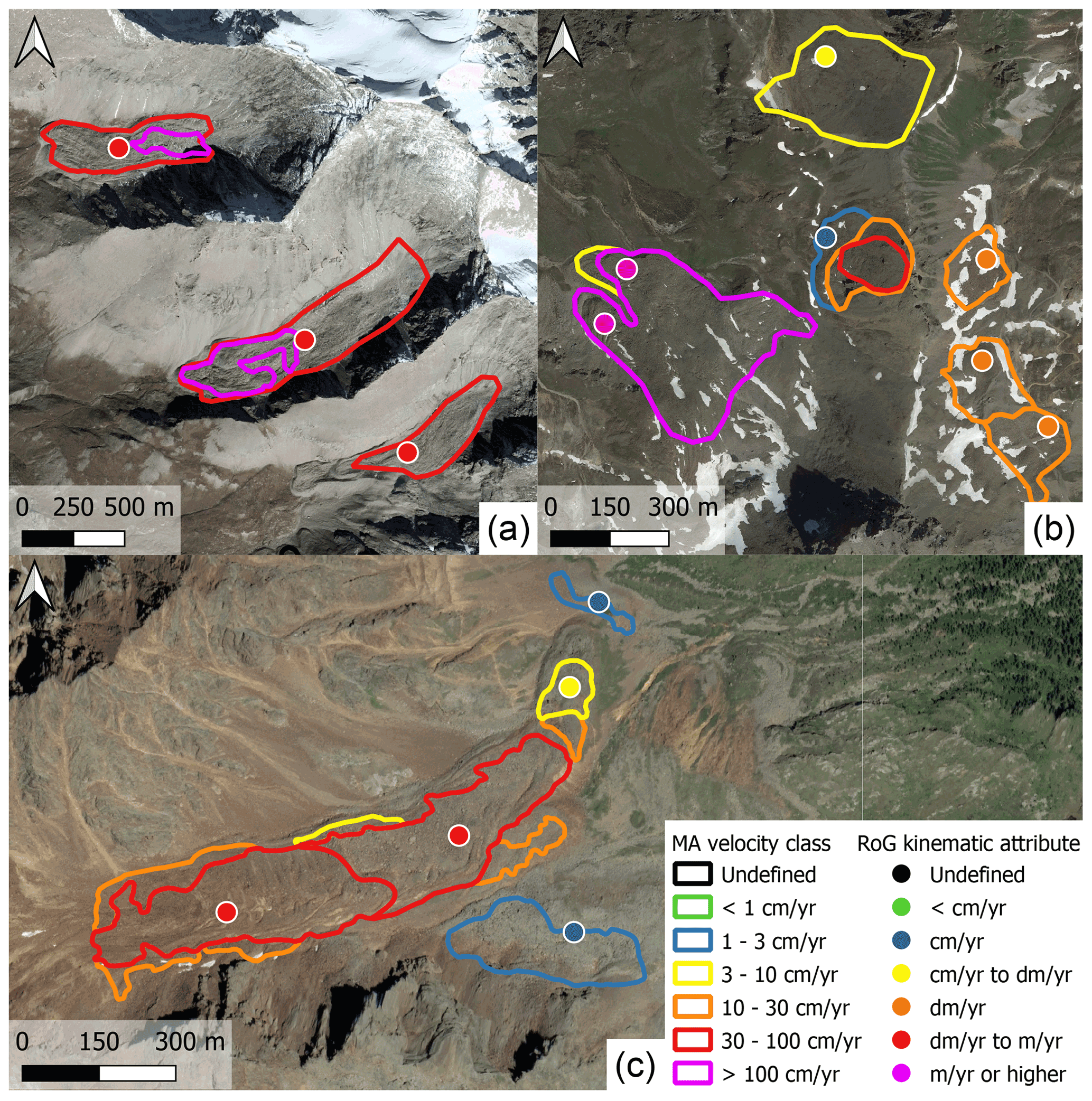
Figure 4Examples of MAs and RoG kinematic attributes produced for Vanoise (a, location: N, E, 2900 m), the western Swiss Alps (b, location: N, E, 2700 m) and southern Venosta (c, location: N, E, 2500 m). Orthoimages from © Google Earth 2019.
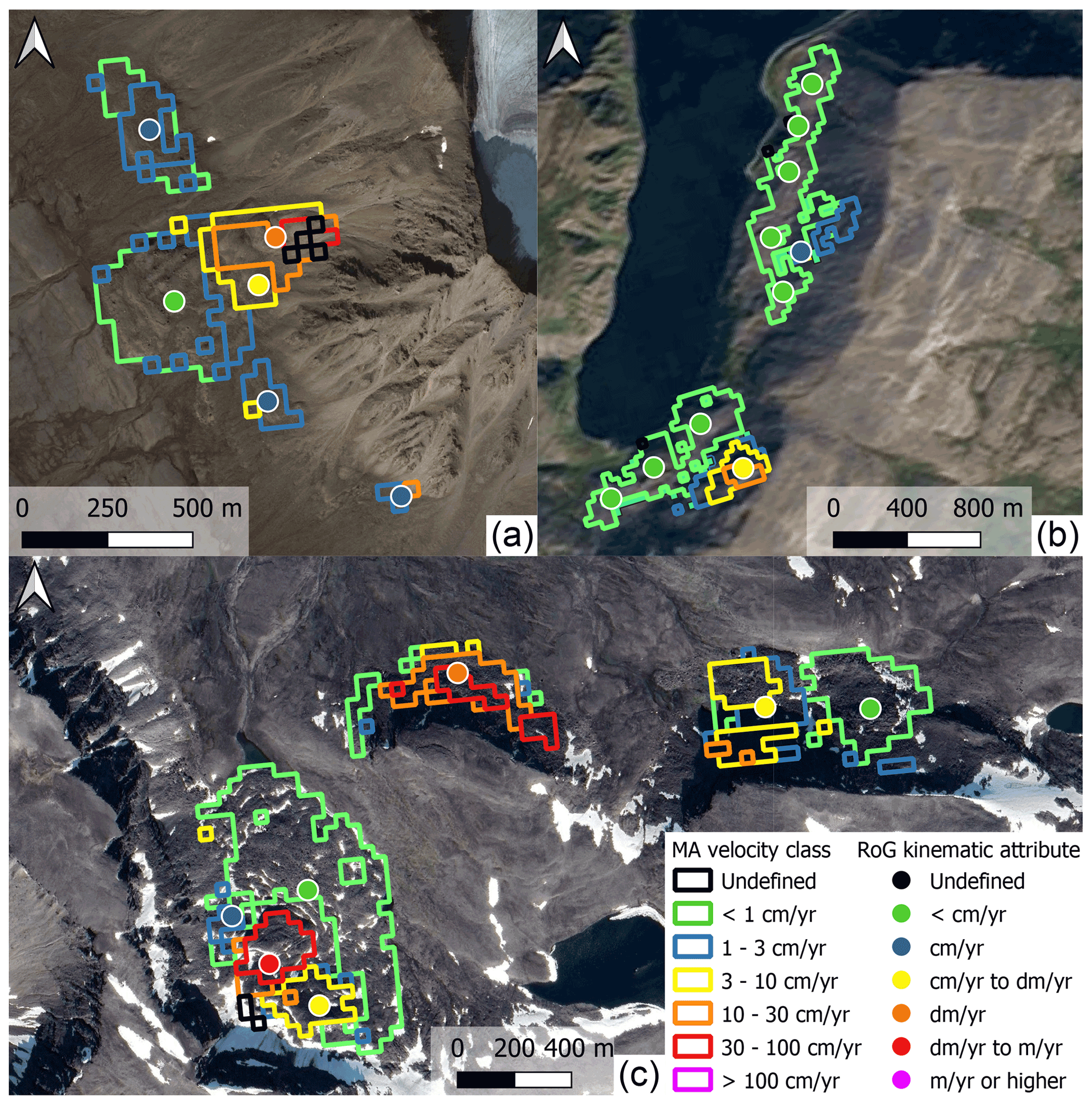
Figure 5Examples of MAs and RoG kinematic attributes produced for Nordenskiöld Land (a, location: N, E, 300 m), Finnmark (b, location: N, E, 100 m) and Troms (c, location: N, E, 920 m) based on a semi-automated multiple temporal baseline InSAR stacking procedure (Rouyet et al., 2021). Orthoimages from Norwegian Mapping Authority (https://www.norgeibilder.no/; last access: 10 October 2021).
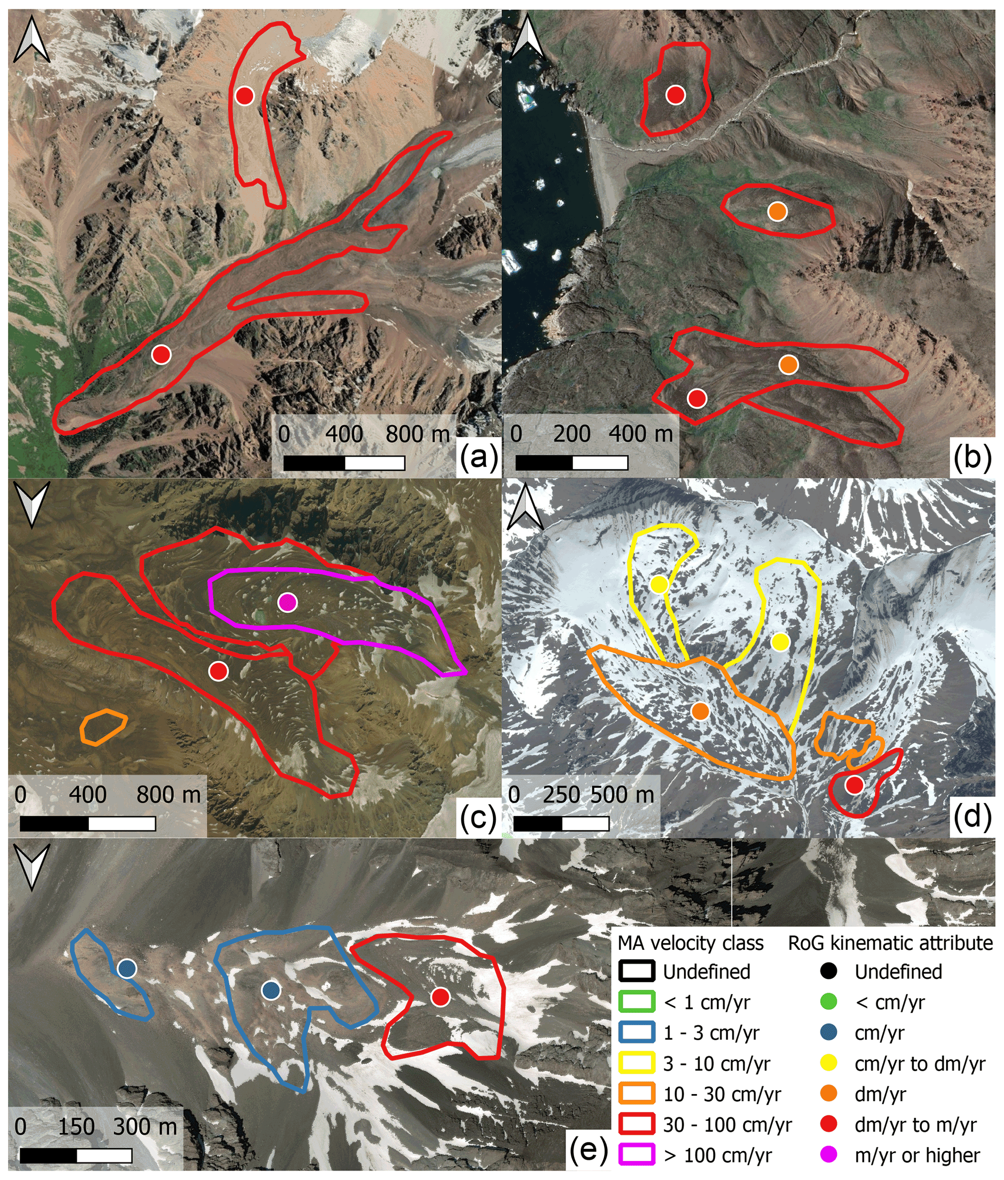
Figure 6Examples of MAs and RoG kinematic attributes produced for the northern Tien Shan (a, location: N, E, 3400 m), Disko Island (b, location: N, W, 100 m), the Central Andes (c, location: S, W, 4400 m), Brooks Range (d, location: N, W, 1700 m) and the central Southern Alps (e, location: S, E, 2000 m). Orthoimages from © Google Earth 2019.
The number of mapped MAs and their extent are quite different between the investigated regions. The number of mapped MAs range from 71 (Finnmark) to 837 (Central Andes), sometime without a proportional increase in the total extent covered by MAs (Figs. 7 and 8a). Central Andes, Disko Island and Brooks Range are the regions with a high number of MAs and a high total extent covered by MAs, while Troms, the western Swiss Alps and southern Venosta have a high number of MAs and a low total extent covered by MAs (Fig. 8a). Accordingly, the first three regions have the largest MAs visible from the boxplots of the area distributions (Fig. 8b), while the last three regions have smaller MAs.

Figure 7Number of inventoried MAs (brown bars) and RoGs classified as undefined (grey bars), relict (green bars), transitional (blue bars) and active (orange bars) for each investigated region. The length of the bars is proportional to the number of observations (x axis). Numbering indicates the total number of MAs and RoGs. Regional inventories are separated according to (i) the method used for mapping the MA (i.e. manual and semi-automated) and (ii) the inclusion or exclusion of relict RoGs. Detailed information on assigned MA velocity classes and RoG kinematic attributes is included in Tables S3 and S4 of the Supplement.
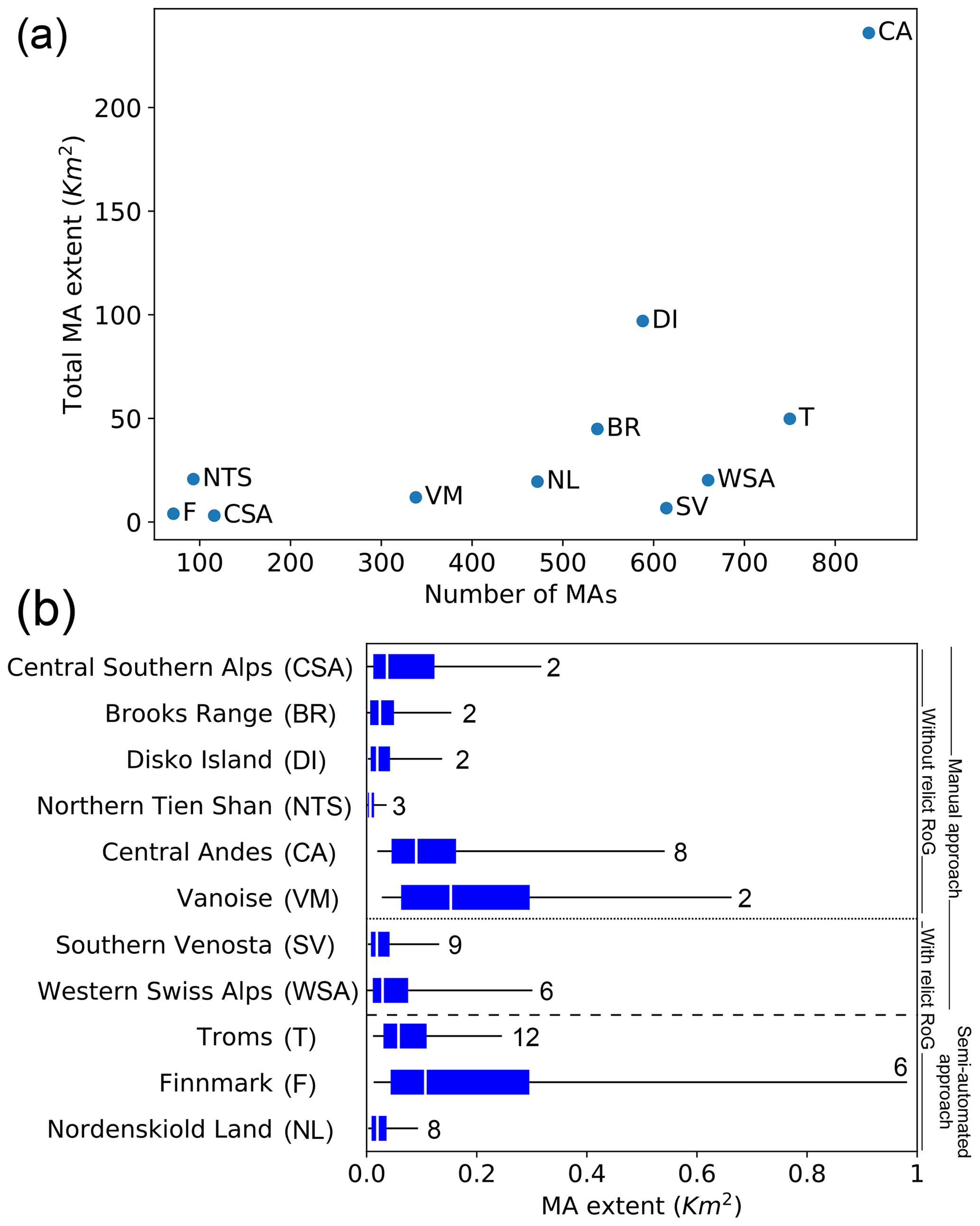
Figure 8(a) Scatterplot of the total area covered by the MAs (y axis) as a function of the number of mapped MAs (x axis). (b) Boxplots show the area distribution of the MAs. Bars enclose interquartile ranges, and whiskers show the 5th and 95th percentiles. On the right, the maximum number of MAs associated with one RoG for each region. Regional inventories are separated according to (i) the method used for mapping the MA (i.e. manual and semi-automated) and (ii) the inclusion or exclusion of relict RoGs.
For the Disko Island, Brooks Range, Vanoise, Central Andes, northern Tien Shan and western Swiss Alps regions, most of the MAs are classified with fast velocity classes (i.e. 30–100 and > 100 cm yr−1; Fig. 9a). In these regions, with the exception of the western Swiss Alps, few MAs (less than 12 %) are classified with slow velocity classes (i.e. < 1 cm yr−1 and/or 1–3 cm yr−1). In the other regions, slow MAs are prevalent, at the expense of faster ones. Therefore, in each region, the faster or slower MAs seem to prevail over their counterparts.
The number of classified RoGs is proportional to the number of detected MAs, but there are fewer RoGs than MAs (Fig. 7). Therefore, this suggests each RoG often contains more than one MA, as illustrated in Fig. 3. The maximum number of MAs associated with a RoG goes up to 12 (Fig. 8b). Southern Venosta, Troms, Nordenskiöld Land and the Central Andes are the regions with the highest number of MAs associated with one RoG, and also with a large number of MAs mapped (Figs. 7 and 8).
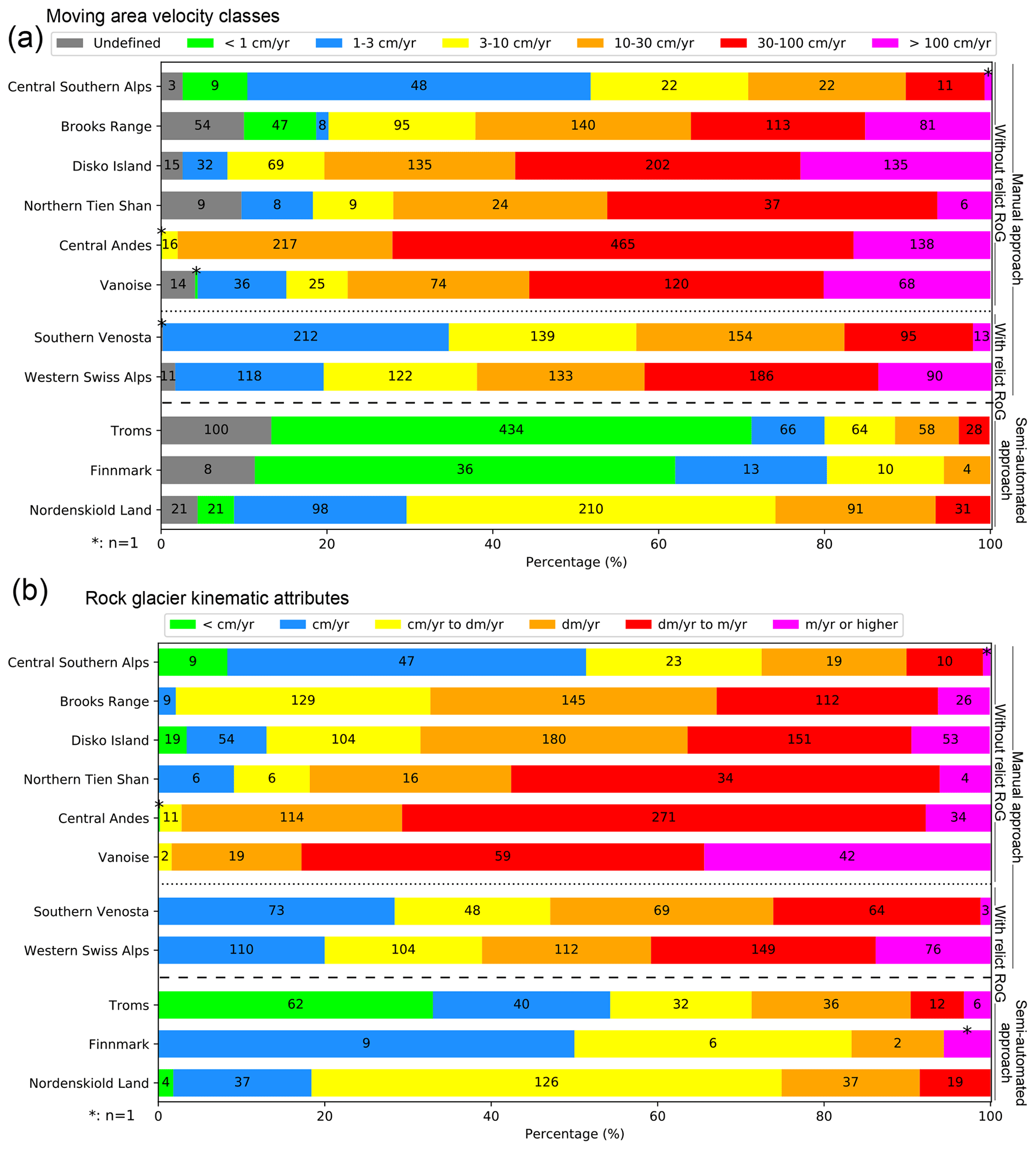
Figure 9Assigned MA velocity classes (a) and RoG kinematic attributes (b) for each investigated region. Relict landforms are not shown in panel (b). The length of the bars is proportional to the percentage (x axis), and the values inside the bars indicate the numbers for each category. Regional inventories are separated according to (i) the method used for mapping the MA (i.e. manual and semi-automated) and (ii) the inclusion or exclusion of relict RoGs. Detailed information on assigned MA velocity classes and RoG kinematic attributes is included in Tables S3 and S4 of the Supplement.
Kinematic attributes are assigned at 3666 RoGs investigated in the study regions. The number of classified RoGs ranges between a maximum of 675 in the Central Andes and a minimum of 57 in Finnmark (Fig. 7). RoGs with an undefined kinematic attribute are less than 15 %, with the exception of the Central Andes (36 %). Most of the RoGs are classified as active and transitional in all the regions investigated, with the exception of Troms (46 %) and Finnmark (32 %). Relict RoGs (i.e. without detected movements) are classified only in Troms (205; 49 %), southern Venosta (60; 18 %), Finnmark (32; 56 %) and the western Swiss Alps (19; 3 %), while in the other regions they are not mapped in this work (Fig. 7) for specific motivations explained below. In the western Swiss Alps region, the initial RoGI used to identify RoGs has been compiled following a “kinematic approach” (RGIK – baseline concepts, 2022), i.e. identifying and inventorying only rock glaciers with a detectable signal of movement, thus excluding relict landforms (Barboux et al., 2015). Consequently, when compiling the kinematic attributes in this region, a limited number of RoGs without detectable movements are classified. In the other regions, the initial inventories used to identify RoGs have been compiled with geomorphological approaches (RGIK – baseline concepts, 2022), i.e. recognising and inventorying rock glaciers by a systematic visual inspection of geomorphological evidence on imaged landscape, DTM-derived products and local field visits, thus including relict landforms (Ellis and Calkin, 1979; Humlum, 1982; Gorbunov, 1983; Mair et al., 2008; Lilleøren and Etzelmüller, 2011; Sattler et al., 2016; Marcer et al., 2017; Zalazar et al., 2020). In the Nordenskiöld Land region – characterised by continuous permafrost – there is no identified relict RoG. In the Vanoise, Brooks Range, Disko Island, northern Tien Shan and Central Andes regions, kinematic analyses are conducted only on landforms identified by a clear InSAR signal of movement, thus without carrying out a thorough and comprehensive kinematic investigation of RoGs and excluding relict landforms. Also for this reason, slow-moving RoGs (i.e. < cm yr−1 and/or cm yr−1) are not mapped in Vanoise, and few slow-moving landforms are classified in the Brooks Range and Central Andes regions (Fig. 9b). In the Brooks Range and Disko Island regions, analyses on RoGs without a clear signal of movement are also not conducted due to the lack of high-resolution optical imagery. In the central Southern Alps, a comprehensive kinematic investigation is conducted, but only RoGs with detectable movements are included in the inventory here presented.
Looking in detail at the classifications, the kinematic attributes of RoGs reflect the velocity classes of MAs, with most RoGs in the Disko Island, Brooks Range, Vanoise, Central Andes, northern Tien Shan, and western Swiss Alps regions classified with fast kinematic attributes (i.e. “dm yr−1 to m yr−1” and “m yr−1 or higher”) and a consistent portion of slow-moving RoGs (i.e. < cm yr−1 and/or cm yr−1) in the other regions (Fig. 9b). In southern Venosta, Troms and Finnmark a large number of slow MAs (i.e. < 1 cm yr−1 and/or 1–3 cm yr−1) are associated with slow-moving RoGs.
Morphological characteristics of RoGs such as the upslope connections are examined, and six main classes of upslope connection are assigned (Fig. 10) according to the IPA baseline concepts: talus, debris mantle, landslide, glacier, glacier forefield and poly connected (i.e. multiple connections) (RGIK – baseline concepts, 2022). An unclear upslope connection is classified as undefined. This classification is not performed in Disko Island and Brooks Range because the available optical data have too low resolution (greater than 10 m) to document this attribute. In the Central Andes region, the classification is not provided because of many cases with unclear upslope connection, and only glacier upslope connection is separated from non-glacier upslope connection. For the western Swiss Alps, southern Venosta, Vanoise, Troms, Finnmark, Nordenskiöld Land and central Southern Alps regions, the highest number of RoGs is classified with an upslope connection of talus type (at least 67 %). Only for the Tien Shan region is the glacier upslope connection type identified as the main class (43 %).
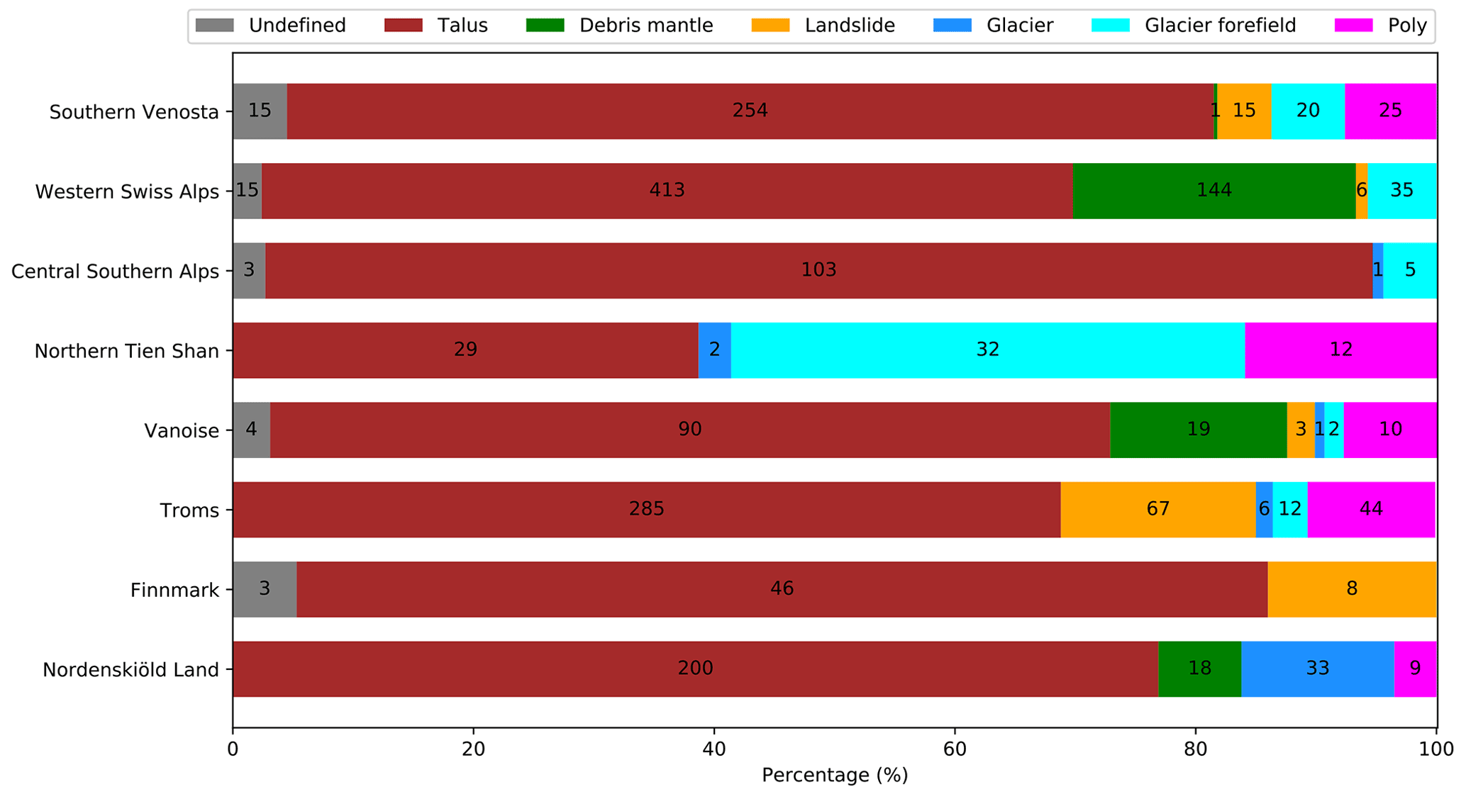
Figure 10Upslope connection classes for most of the investigated regions. The size of the horizontal bars is proportional to the percentage (x axis), and the values inside the bars are the numbers for each upslope connection class. The Disko Island and Brooks Range regions are not shown because of lack of high-resolution optical data needed to document this attribute. The Central Andes region is not shown because of many cases with undefined upslope connection.
The validation of the assigned kinematic information is conducted on 30 RoGs with available DGNSS and feature tracking measurements acquired during the same time frame of InSAR measurements. The assigned MA velocity classes sometimes do not fully cover the velocity ranges recorded by DGNSS measurements (Table 3). For 24 RoGs, the assigned kinematic attributes are in agreement with the available kinematic measurements. For four RoGs the assigned kinematics are slightly underestimated with InSAR, and for two RoGs the kinematics are slightly overestimated (Table 3). Detailed results obtained from the validation are included in Supplement Sect. B “Description of conducted validation”.
Table 3Validation conducted between the detected kinematic information (i.e. MA velocity classes and RoG kinematic attributes) and the independent datasets available for some regions.

5.1 Subjectivity of the method
The main problem for integrating standardised kinematic information within inventories compiled from different operators is the subjectivity of the operator in carrying out the work. The inherent degree of subjectivity is a typical source of uncertainty and variability within inventories compiled from remotely sensed imagery (Jones et al., 2018a; Brardinoni et al., 2019). The proposed guidelines contain specific rules to guide the operator and reduce the operator's freedom to make specific choices, thus limiting the subjectivity. Unlike other techniques, the InSAR signal provides an accurate measurement of movement, but the interpretation of the signal can still be affected by some degree of variability. Therefore, multiple phases of correction and adjustment were conducted by a second operator to further reduce the subjectivity and increase the overall reliability of the results. In addition, the assigned MA velocity classes and RoG kinematic attributes refer to a range and not a precise value, which contributes to further reduce the degree of subjectivity.
Despite the guidelines adopted, some degree of subjectivity can still occur. A large heterogeneity of the kinematics is often related to large spatial and temporal variability of the InSAR signal, interpreted in different ways by the operators. Therefore, before starting the work on the 11 investigated sites, the operators independently tested the guidelines on two regions in the western Swiss Alps. Such an inter-comparison exercise has shown to be a useful approach to evaluate the operator subjectivity (Brardinoni et al., 2019). Results of this inter-comparison exercise are included in a specific document of the ESA Permafrost_CCI project (ESA – PVIR report, 2021). Outcomes show an increase in variability (i) in delineation and velocity classification of MAs affected by large temporal and spatial variations in interferograms and (ii) in the kinematic classification of RoGs affected by a greater velocity heterogeneity of the related MAs. However, often the same landforms have been classified with similar or adjacent classes, especially for fast landforms, because fast-moving classes include wider velocity ranges than slow-moving classes with smaller velocity ranges (ESA – PVIR report, 2021). Two examples are included in this paper (Fig. 11) to show the contrast between a simple RoG and a more complex one, characterised by higher variability of InSAR data. Results of the inter-comparison exercise were also useful in establishing stricter and clearer rules to further reduce the subjectivity and releasing the most refined version of the guidelines presented here. Furthermore, this initial stage conducted on two limited regions improved the knowledge and confidence of the method proposed by researchers.
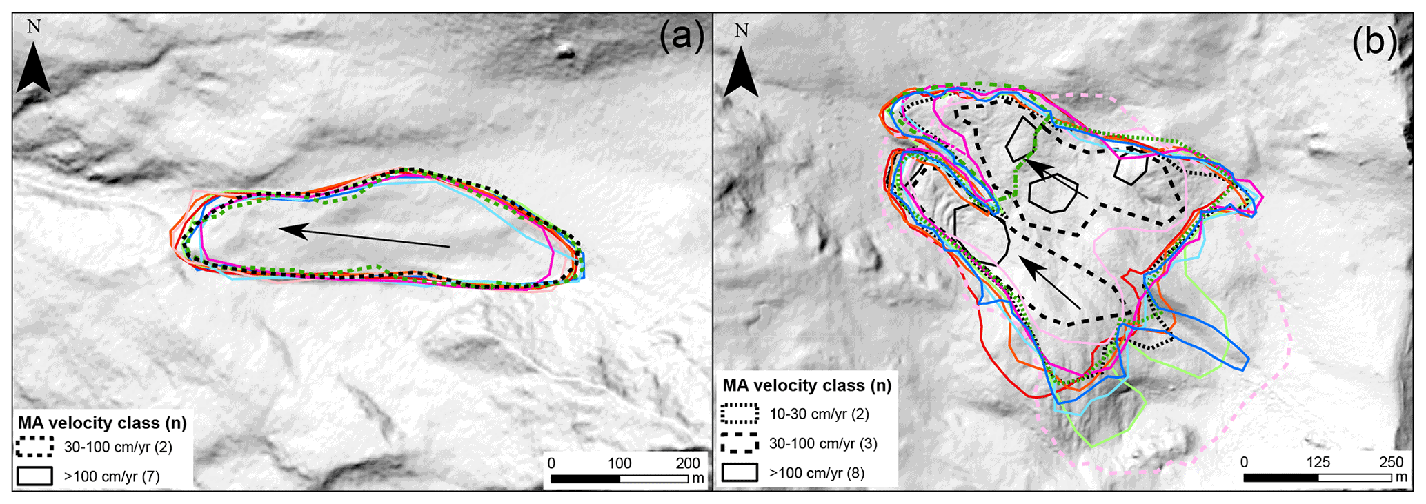
Figure 11Two examples (a, b) of MAs delineated by nine operators. Hillshade as background from Swisstopo© (https://www.swisstopo.admin.ch; last access: 10 October 2021). The outlines drawn on the simple RoG (a) are very similar, and MAs are classified as > 100 cm yr−1 by seven operators and as 30–100 cm yr−1 by two operators, due to temporal variations in interferograms. According to the mapped MAs, this RoG is classified as m yr−1 or higher (also in agreement to GNSS data) by seven operators and as dm yr−1 to m yr−1 by two operators. Greater heterogeneity is observed on RoG affected by larger temporal and spatial variations in interferograms (b), with more heterogeneous outlines of MAs and different assigned velocity classes (> 100, 30–100 and 10–30 cm yr−1). However, despite the larger heterogeneity, this RoG is classified as m yr−1 or higher by six operators and as dm yr−1 to m yr−1 by three operators; these kinematic attributes are in line with GNSS data, ranging from about 0.2 to 2 m yr−1. Some related interferograms are included in Figs. S2–S4 of the Supplement.
5.2 Dependencies related to moving-area inventories
The guidelines presented here define rules that can be followed using different remote sensing techniques. In this work we used the InSAR technology, and therefore moving-area inventories are affected by limitations related to radar interferometry (Klees and Massonnet, 1998; Barboux et al., 2014; Strozzi et al., 2020). The use of the same sensors (i.e. Sentinel-1 and ALOS-2) that share the same technical limits in all the investigated regions, however, simplifies the evaluation between the moving-area inventories.
The first limit related to InSAR is the general underestimation of displacements measured in the MAs (Klees and Massonnet, 1998; Massonnet and Souyris, 2008). The downslope direction is generally assumed to represent the real 3D movement of RoGs (Barboux et al., 2014); therefore the magnitude of displacement of MAs on north- and south-facing slopes is more underestimated, even if both ascending and descending geometries are used.
The second limit related to InSAR concerns MAs with slow movements (i.e. with velocities slower than 3 cm yr−1), mainly investigated using annual interferograms with Sentinel-1 and ALOS-2 (Barboux et al., 2014; Yague-Martinez et al., 2016). With long time intervals (i.e. annual), the quality of the interferograms is lower due to loss of phase coherence (Klees and Massonnet, 1998; Touzi et al., 1999; Barboux et al., 2014; Bertone et al., 2019). Slow movements are therefore more complicated to assess with enough precision, and the reliability is consequently lower. For this reason, (i) the faster MAs seem to prevail over their counterparts in some regions (Fig. 9a), and (ii) MAs with the velocity class < 1 cm yr−1 are probably not mapped in the Central Andes, northern Tien Shan, Disko Island, Vanoise, southern Venosta and Swiss Alps regions (Fig. 9a), where the focus is set on the more active landforms. In the Troms and Finnmark regions, the large number of slow MAs is related to the semi-automated method used, able to better derive slow movements by exploiting a large set of interferograms with long time intervals.
Despite the limitations, InSAR is an appropriate tool for this exercise aimed at compiling kinematic inventories in as many representative periglacial regions worldwide as possible (Yague-Martinez et al., 2016). The InSAR image processing effort has been split across many sites. More advanced interferometric processing strategies such as persistent scatterer interferometry (Ferretti et al., 2001; Crosetto et al., 2016; Wangchuk et al., 2022) would allow the derivation of slow surface motion precisely, but the processing load is much more significant, and special attention has to be paid to the long-lasting snow cover and the atmospheric stratification at high altitudes (Barboux et al., 2015; Osmanoğlu et al., 2016).
To reduce the intrinsic limitations of InSAR, additional or alternative techniques may be used to support kinematic classification. For example, feature tracking (Monnier and Kinnard, 2017) and image cross correlation (Kääb, 2002; Necsoiu et al., 2016; Kääb et al., 2021) conducted on high-resolution optical imagery acquired from airborne or spaceborne platforms represent viable alternatives or complements to obtaining kinematic information on large areas. Similarly, the differencing of sequential high-resolution DTMs has been successfully used to quantify surface displacement and vertical change in particular (Kääb, 2008; Avian et al., 2009). These techniques, although extremely useful for detecting large movements (i.e. topographic changes) with high accuracy over seasonal to annual and decadal timescales, rely heavily on the timing of costly repeat surveys, which typically have lower temporal resolution compared to SAR satellite-based acquisitions.
5.3 Characteristics related to the kinematics of rock glaciers
The guidelines used for assigning kinematic attributes to RoGs aim to be technology independent. However, (i) the kinematic information assigned refers only to periods documented by InSAR data (snow-free seasons) and (ii) the inherent dynamic characteristics of the RoG can have impacts on the results. The seasonal variability (Berger et al., 2004; Delaloye and Staub, 2016; Wirz et al., 2016; Kenner et al., 2017; Cicoira et al., 2019) is considered when the velocity classes of MAs assigned during an observation time window of a few months are converted to kinematic attributes of RoGs (the latter refer to a multi-annual validity time frame, Table 2). However, the kinematic information might still be overestimated in cases where the RoG undergoes a strong seasonal acceleration. Furthermore, due to the observation time window of a few months (snow-free periods), local effects such as residual snow can further reduce the amount of available interferometric data. Coherent 6 d winter interferograms with Sentinel-1 could be used in the future to highlight the seasonal fluctuations (Strozzi et al., 2020).
In addition to the kinematic information, the high-quality optical data and the investigated connections of RoGs with other landforms (Fig. 10) provide useful information (Seppi et al., 2012; Necsoiu et al., 2016; Kääb et al., 2021; RGIK – baseline concepts, 2022). For example, in glacier-connected and glacier-forefield-connected landforms, the distinction between rock glaciers and debris-covered glaciers is sometimes complicated (Berger et al., 2004; Bosson and Lambiel, 2016; Bolch and Marchenko, 2019; Robson et al., 2022), and analyses of high-quality optical data help to discriminate the upper glacial part from the real lower rock glacier part. In the Central Andes region – where the upslope connections are often unclear – the distinctions between RoGs and debris-covered glaciers have not always been possible. Furthermore, the identification of glacier-connected and glacier-forefield-connected rock glaciers is important to interpret the kinematic information, because these landforms are frequently characterised by ice melting that induces subsidence in summer (Delaloye and Staub, 2016). The portion of RoGs potentially affected by consistent subsidence (i.e. glacier and glacier-forefield upslope connected) is however lower than 13 % in the investigated regions, except in the northern Tien Shan region where it is around 45 %.
5.4 Kinematic analysis of produced moving areas and rock glaciers
In the study regions, a total of 5077 MAs were inventoried. These provide information on surface deformation associated with RoG activity. Application of manual and semi-automated methods has yielded some differences. We observe fragmented MA outlines that reflect the jagged edges of pixels (down to single-pixel MAs) in Norway and Svalbard (Rouyet et al., 2021), whereas manually smoothed outlines characterise the MAs in the other study regions. Clearly, MAs obtained with the semi-automated method (based on averaged unwrapped interferograms) are not directly comparable with manual counterparts (based on visual inspection of wrapped interferograms). The choice between manual and semi-automated methods should be made according to the regional extent and the available time, favouring semi-automated methods mainly for very large regions, where manual approaches take too much time.
Despite the slight differences detected in the moving-area inventories, the kinematic attributes were successfully assigned to 3666 RoGs, exploiting standardised rules to translate kinematic information from MAs to RoGs. The main discrepancies are related to the absence of RoGs classified as relict in the Vanoise, Disko Island, Brooks Range, northern Tien Shan, Central Andes and central Southern Alps regions (Fig. 7). Only the southern Venosta, Troms and Finnmark regions include a consistent number of RoGs without detectable movements. In the western Swiss Alps, relict RoGs were not mapped because the method used to produce the RoGI excludes the landforms without movement. Therefore, the completeness of the inventories used to identify RoGs is essential to obtain a thorough and comprehensive kinematic investigation. In the Vanoise, Disko Island, Brooks Range, northern Tien Shan, Central Andes and central Southern Alps regions relict RoGs were not classified because the mapping effort was placed only on faster-moving landforms. The choice not to carry out analyses on RoGs without a clear signal of movement in these regions is due to two reasons. First, the aim of this approach is to implement the kinematic information on RoGs in an active state, without paying too much attention to the slowest landforms. Second, RoGs without movements or with slow movements are more difficult to investigate because the quality of the InSAR signal of yearly interferograms is generally lower (Touzi et al., 1999; Barboux et al., 2014; Bertone et al., 2019). Consequently, relict and slow-moving RoGs are more easily omitted or classified as undefined. For the above reasons, some compiled inventories only provide preliminary results, which still need some improvements to be fully comprehensive. However, the use of InSAR data allowed the update of the inventories, leading to a more accurate classification, especially for active and transitional landforms.
The results show a number of challenges that need to be addressed by the scientific community. For this reason, it is not possible to conduct detailed interpretations and comparisons between the investigated regions, which would require further investigations. However, we discuss some preliminary considerations below. We observed a large number of fast-moving RoGs (i.e. with kinematic attributes of dm yr−1 to m yr−1 and m yr−1 or higher) in the Vanoise, Central Andes and northern Tien Shan regions (Fig. 9b). Higher velocities of rock glaciers in the northern Tien Shan and Central Andes than in the Alps have already been observed (Roer et al., 2005; Kääb et al., 2021; Gorbunov, et al., 1992). However, as already documented by other authors (Roer et al., 2008; Delaloye et al., 2010, 2013; Delaloye and Staub, 2016; Marcer et al., 2019; Seppi et al., 2019), there are also fast-moving rock glaciers situated on steep slopes in the Alps. In Troms, Finnmark and Nordenskiöld Land, the high number of slow-moving RoGs (i.e. < cm yr−1, cm yr−1 and cm yr−1 to dm yr−1) has also been observed in other studies (Rouyet et al., 2019; Lilleøren et al., 2022). In contrast, little attention had been paid to the dynamics and evolution of rock glaciers in the Brooks Range, Disko Island and central Southern Alps regions (Calkin, 1987; Sattler et al., 2016). This work therefore presents the first results on the kinematics of RoGs in these study areas.
The quality of the assigned kinematic information was evaluated according to recent work (Strozzi et al., 2020; Kääb et al., 2021) on 30 landforms in all the investigated regions, except for southern Venosta, Finnmark and Disko Island (Table 3). With reference to the main objective of this work, which is assigning a robust and reproducible kinematic attribute to RoGs, our classification resulted in being correct in most cases. The four landforms underestimated may be related to the limits of the InSAR technique, such as the LOS orientation explained above, which generates underestimation in particular on north- and south-facing slopes. On the other hand, the two landforms overestimated may be related to the high seasonal variability of RoGs and the different observation time windows used to measure the movements between InSAR (i.e. summer) and the validation dataset (i.e. annual). As explained above, the seasonal variability is considered when the velocity classes of MAs are converted to kinematic attributes of RoGs. However, if the RoG undergoes a strong seasonal acceleration, the assigned kinematic attributes might still be higher than the kinematic information available from the validation dataset.
5.5 Further application potential
This method holds potential for gaining new insight into RoG dynamics at a global scale. The spatial distribution of rock glaciers is frequently used as a proxy for the past or present occurrence of permafrost (Haeberli, 1985; Boeckli et al., 2012; Schmid et al., 2015; Marcer et al., 2017), and the kinematics of these landforms can be used to derive indirect information about permafrost state. The methodology proposed in this work promotes the assignment of standardised kinematic attributes to RoGs and therefore fosters the compilation of consistent information on permafrost at a global scale. Possible applications that will benefit from the proposed approach include the calibration of permafrost numerical models (Cremonese et al., 2011; Boeckli et al., 2012; Lilleøren et al., 2013; Schmid et al., 2015; Sattler et al., 2016; Marcer et al., 2017; Westermann et al., 2017) and artificial intelligence algorithms for assessing rock glacier activity over large areas (Frauenfelder et al., 2008; Boeckli et al., 2012; Kofler et al., 2020; Robson et al., 2020). Furthermore, indirect information on ice content within rock glaciers (Schmid et al., 2015; Marcer et al., 2017) may be used for improved water storage estimation, which so far is based only on rough estimates (Bolch et al., 2009; Jones et al., 2018a).
The kinematic attributes assigned in this work are not intended for any monitoring purpose. In most cases, the kinematics of the rock glacier do not change much over the decades, and a change by more than one kinematic class is unlikely to occur. Monitoring activities on rock glaciers are conducted using specific and more precise techniques (Delaloye et al., 2013; Fey and Krainer, 2020; Strozzi et al., 2020; Kääb et al., 2021). In this context, the approach here described can support (i) the identification of sites to start monitoring activities and (ii) the large-scale assessment to identify RoGs that may be a source of natural hazard (Delaloye et al., 2013; Kummert et al., 2018).
The method and the products presented here are the first results of an internationally coordinated work in which researchers from nine institutes applied common guidelines to 11 regions worldwide, using spaceborne interferometric synthetic aperture radar measurements, to systematically integrate kinematic information within RoGIs. Periglacial regions with different environmental settings in both the Northern Hemisphere and Southern Hemisphere have been investigated. Despite the regional heterogeneity and the intensive manual effort, the definition and application of common rules to include a RoG kinematic attribute within inventories have been feasible. It was possible to assign kinematic information to a majority of the investigated RoGs. However, in some regions, a larger number of landforms need to be validated, and RoGs with slow movements or without movements require further investigation. The promising results derived from the application of the InSAR-based standardised procedure open up new possibilities for understanding rock glacier dynamics and the impact of climate change on permafrost degradation. Currently, these tasks are mainly based on in situ measurements of a limited number of landforms. The compiled inventories, even if still preliminary, will provide valuable data for training, validation and testing of artificial intelligence and numerical modelling algorithms on rock glaciers using satellite imagery.
Further research – in both remote-sensing- and fieldwork-based approaches – is needed to reduce the limitations associated with InSAR. Both the guidelines and the inventories still need improvement, and more advanced InSAR processing strategies such as multi-temporal interferometric approaches, or different remote sensing technologies such as feature tracking on optical airborne images, could be applied. The lessons learned from the current study are critical in refining the proposed method and applying it widely to more regions.
The produced inventories are available at https://unifr.maps.arcgis.com/apps/instant/portfolio/index.html?appid=99cf50eb91c245d1b171a4a842d8ef0e (Bertone et al., 2021).
The Supplement includes the description of study areas (Sect. A), the tables of the attributes assigned to the MAs (Table S1) and RoGs (Table S2), examples of MAs classification (Fig. S1), detailed tables of the MA velocity classes (Table S3) and RoG kinematic attributes (Table S4), the description of the conducted validation (Sect. B), and examples of subjectivity observed (Figs. S2, S3 and S4). The supplement related to this article is available online at: https://doi.org/10.5194/tc-16-2769-2022-supplement.
CB, RD, LR and TS designed the study and managed the project. AB analysed data and wrote the manuscript. CB, RD, LiR and TS contributed to data analysis and wrote the manuscript. AB, CB, XB, TB, FB, RC, HHC, MDD, RD, BE, OH, CL, KSL, GP, LR and LuR produced the inventories. TS and LiR produced the interferometric data. All authors contributed to the writing of the final version of the paper.
The authors declare that the research was conducted in the absence of any commercial or financial relationships that could be construed as a potential conflict of interest. Some authors are members of the editorial board of The Cryosphere. The peer-review process was guided by an independent editor.
Publisher's note: Copernicus Publications remains neutral with regard to jurisdictional claims in published maps and institutional affiliations.
The SAR data were processed with Gamma software. Moving-area inventories and RoG data were produced by the authors involved in this work. We thank the editor, the co-editor and the reviewers for their critical work, which has allowed a considerable improvement of the paper.
This research was funded by the European Space Agency Permafrost_CCI project (grant number 4000123681/18/I-NB).
This paper was edited by Christian Hauck and reviewed by Jan Henrik Blöthe and one anonymous referee.
Avian, M., Kellerer-Pirklbauer, A., and Bauer, A.: LiDAR for monitoring mass movements in permafrost environments at the cirque Hinteres Langtal, Austria, between 2000 and 2008, Nat. Hazards Earth Syst. Sci., 9, 1087–1094, https://doi.org/10.5194/nhess-9-1087-2009, 2009.
Azócar, G. F. and Brenning, A.: Hydrological and geomorphological significance of rock glaciers in the dry Andes, Chile (27–33 S), Permafrost Periglac., 21, 42–53, 2010.
Barboux, C., Delaloye, R., and Lambiel, C.: Inventorying slope movements in an Alpine environment using DInSAR, Earth Surf. Proc. Land., 39, 2087–2099, https://doi.org/10.1002/esp.3603, 2014.
Barboux, C., Strozzi, T., Delaloye, R., Wegmüller, U., and Collet, C.: Mapping slope movements in Alpine environments using TerraSAR-X interferometric methods, ISPRS J. Photogramm., 109, 178–192, https://doi.org/10.1016/j.isprsjprs.2015.09.010, 2015.
Barcaza, G., Nussbaumer, S. U., Tapia, G., Valdés, J., García, J.-L., Videla, Y., Albornoz, A., and Arias, V.: Glacier inventory and recent glacier variations in the Andes of Chile, South America, Ann. Glaciol., 58, 166–180, 2017.
Barsch, D.: Permafrost creep and rockglaciers, Permafrost Periglac., 3, 175–188, https://doi.org/10.1002/PPP.3430030303, 1992.
Barsch, D.: Rockglaciers: indicators for the Permafrost and Former Geoecology in High Mountain Environment, Springer Sci., Berlin, Heidelberg, Germany, 1996.
Berger, J., Krainer, K., and Mostler, W.: Dynamics of an active rock glacier (Ötztal Alps, Austria), Quaternary Res., 62, 233–242, https://doi.org/10.1016/j.yqres.2004.07.002, 2004.
Berthling, I.: Beyond confusion: Rock glaciers as cryo-conditioned landforms, Geomorphology, 131, 98–106, https://doi.org/10.1016/J.GEOMORPH.2011.05.002, 2011.
Bertone, A., Zucca, F., Marin, C., Notarnicola, C., Cuozzo, G., Krainer, K., Mair, V., Riccardi, P., Callegari, M., and Seppi, R.: An Unsupervised Method to Detect Rock Glacier Activity by Using Sentinel-1 SAR Interferometric Coherence: A Regional-Scale Study in the Eastern European Alps, Remote Sens., 11, 1711, https://doi.org/10.3390/rs11141711, 2019.
Bertone, A., Barboux, C., Bodin, X., Bolch, T., Brardinoni, F., Caduff, R., Christiansen, H. H., Darrow, M., Delaloye, R., Etzelmüller, B., Humlum, O., Lambiel, C., Lilleøren, K. S., Mair, V., Pellegrinon, G., Rouyet, L., Ruiz, L., and Strozzi, R.: Regional kinematics-based rock glacier inventories (ESA CCI+ Permafrost project), https://unifr.maps.arcgis.com/apps/instant/portfolio/index.html?appid=99cf50eb91c245d1b171a4a842d8ef0e, last access: 12 October 2021.
Blöthe, J. H., Rosenwinkel, S., Höser, T., and Korup, O.: Rock-glacier dams in High Asia, Earth Surf. Proc. Land., 44, 808–824, https://doi.org/10.1002/esp.4532, 2019.
Blöthe, J. H., Halla, C., Schwalbe, E., Bottegal, E., Trombotto Liaudat, D., and Schrott, L.: Surface velocity fields of active rock glaciers and ice-debris complexes in the Central Andes of Argentina, Earth Surf. Proc. Land., 46, 504–522, 2021.
Boeckli, L., Brenning, A., Gruber, S., and Noetzli, J.: A statistical approach to modelling permafrost distribution in the European Alps or similar mountain ranges, The Cryosphere, 6, 125–140, https://doi.org/10.5194/tc-6-125-2012, 2012.
Bolch, T. and Gorbunov, A. P.: Characteristics and origin of rock glaciers in northern Tien Shan (Kazakhstan/Kyrgyzstan), Permafrost Periglac., 25, 320–332, https://doi.org/10.1002/ppp.1825, 2014.
Bolch, T. and Strel, A.: Evolution of rock glaciers in northern Tien Shan, Central Asia, 1971–2016, in: 5th European Conference on Permafrost, Chamonix, France, 23 June–1 July 2018, 48–49, 2018.
Bolch, T. and Marchenko, S. S.: Significance of glaciers, rockglaciers and ice-rich permafrost in the Northern Tien Shan as water towers under climate change conditions, in: Selected papers from the Workshop “Assessment of Snow, Glacier and Water Resources in Asia” held in Almaty, Kazakhstan, 28–30 November 2006, IHP/HWRP-Berichte, 8, 132–144, 2009.
Bolch, T., Rohrbach, N., Kutuzov, S., Robson, B. A., and Osmonov, A.: Occurrence, evolution and ice content of ice-debris complexes in the Ak-Shiirak, Central Tien Shan revealed by geophysical and remotely-sensed investigations, Earth Surf. Proc. Land., 44, 129–143, https://doi.org/10.1002/esp.4487, 2019.
Bosson, J.-B. and Lambiel, C.: Internal Structure and Current Evolution of Very Small Debris-Covered Glacier Systems Located in Alpine Permafrost Environments, Front. Earth Sci., 4, 39, https://doi.org/10.3389/feart.2016.00039, 2016.
Brardinoni, F., Scotti, R., Sailer, R., and Mair, V.: Evaluating sources of uncertainty and variability in rock glacier inventories, Earth Surf. Proc. Land., 44, 2450–2466, https://doi.org/10.1002/esp.4674, 2019.
Brencher, G., Handwerger, A. L., and Munroe, J. S.: InSAR-based characterization of rock glacier movement in the Uinta Mountains, Utah, USA, The Cryosphere, 15, 4823–4844, https://doi.org/10.5194/tc-15-4823-2021, 2021.
Calkin, P. E.: Rock glaciers of central Brooks Range, Alaska, USA, Rock Glaciers, Allen and Unwin, London, 65–82, 1987.
Charbonneau, A. A. and Smith, D. J.: An inventory of rock glaciers in the central British Columbia Coast Mountains, Canada, from high resolution Google Earth imagery, Arctic, Antarct. Alp. Res., 50, 1489026, https://doi.org/10.1080/15230430.2018.1489026, 2018.
Cicoira, A., Beutel, J., Faillettaz, J. and Vieli, A.: Water controls the seasonal rhythm of rock glacier flow, Earth Planet. Sc. Lett., 528, 115844, https://doi.org/10.1016/J.EPSL.2019.115844, 2019.
Colucci, R. R., Boccali, C., Žebre, M., and Guglielmin, M.: Rock glaciers, protalus ramparts and pronival ramparts in the south-eastern Alps, Geomorphology, 269, 112–121, https://doi.org/10.1016/j.geomorph.2016.06.039, 2016.
Corte, A.: The hydrological significance of rock glaciers, J. Glaciol., 17, 157–158, 1976.
Cremonese, E., Gruber, S., Phillips, M., Pogliotti, P., Boeckli, L., Noetzli, J., Suter, C., Bodin, X., Crepaz, A., Kellerer-Pirklbauer, A., Lang, K., Letey, S., Mair, V., Morra di Cella, U., Ravanel, L., Scapozza, C., Seppi, R., and Zischg, A.: Brief Communication: ”An inventory of permafrost evidence for the European Alps”, The Cryosphere, 5, 651–657, https://doi.org/10.5194/tc-5-651-2011, 2011.
Crosetto, M., Monserrat, O., Devanthéry, N., Cuevas-González, M., Barra, A., and Crippa, B.: Persistent scatterer interferometry using Sentinel-1 data, Int. Arch. Photogramm. Remote, 41, 835–839, https://doi.org/10.5194/isprsarchives-XLI-B7-835-2016, 2016.
Darrow, M. M., Gyswyt, N. L., Simpson, J. M., Daanen, R. P., and Hubbard, T. D.: Frozen debris lobe morphology and movement: an overview of eight dynamic features, southern Brooks Range, Alaska, The Cryosphere, 10, 977–993, https://doi.org/10.5194/tc-10-977-2016, 2016.
Delaloye, R. and Staub, B.: Seasonal variations of rock glacier creep: Time series observations from the Western Swiss Alps, in: Proceedings of the International Conference on Book of Abstracts, Potsdam, Germany, hdl:10013/epic.49110, 20–24 June 2016.
Delaloye, R., Lambiel, C., and Gärtner-Roer, I.: Overview of rock glacier kinematics research in the Swiss Alps, Geogr. Helv., 65, 135–145, https://doi.org/10.5194/gh-65-135-2010, 2010.
Delaloye, R., Morard, S., Barboux, C., Abbet, D., Gruber, V., Riedo, M., and Gachet, S.: Rapidly moving rock glaciers in Mattertal, Jahrestagung der Schweizerischen Geomorphol. Gesellschaft, 29, 21–31, 2013.
Delaloye, R., Barboux, C., Bodin, X., Brenning, A., Hartl, L., Hu, Y., Ikeda, A., Kaufmann, V., Kellerer-Pirklbauer, A., and Lambiel, C.: Rock glacier inventories and kinematics: A new IPA Action Group, in: Eucop5–5th European Conference of Permafrost, Chamonix, France, 23 June–1 July 2018, 23, 392–393, 2018.
Ellis, J. M. and Calkin, P. E.: Nature and distribution of glaciers, neoglacial moraines, and rock glaciers, east-central Brooks Range, Alaska, Arctic Alpine Res., 11, 403–420, 1979.
Eriksen, H. Ø., Rouyet, L., Lauknes, T. R., Berthling, I., Isaksen, K., Hindberg, H., Larsen, Y., and Corner, G. D.: Recent acceleration of a rock glacier complex, Adjet, Norway, documented by 62 years of remote sensing observations, Geophys. Res. Lett., 45, 8314–8323, 2018.
ESA – PVIR report: ESA CCI+ Permafrost, CCN1 & CCN2 Rock Glacier Kinematics as New Associated Parameter of ECV Permafrost, D4.1 Product Validation and Intercomparison Report (PVIR), https://climate.esa.int/media/documents/CCI_PERMA_CCN1_2_D4.1_PVIR_v1.0_20210127.pdf, last access: 12 October 2021.
Falaschi, D., Tadono, T,. and Masiokas, M.: Rock glaciers in the patagonian andes: an inventory for the monte san lorenzo (cerro cochrane) massif, 47degrees, Geogr. Ann. Ser. A, 97, 769–777, https://doi.org/10.1111/geoa.12113, 2015.
Ferretti, A., Prati, C., and Rocca, F.: Permanent scatterers in SAR interferometry, IEEE T. Geosci. Remote, 39, 8–20, https://doi.org/10.1109/36.898661, 2001.
Fey, C. and Krainer, K.: Analyses of UAV and GNSS based flow velocity variations of the rock glacier Lazaun (Ötztal Alps, South Tyrol, Italy), Geomorphology, 365, 107261, https://doi.org/10.1016/j.geomorph.2020.107261, 2020.
Frauenfelder, R., Schneider, B., and Kääb, A.: Using dynamic modelling to simulate the distribution of rockglaciers, Geomorphology, 93, 130–143, https://doi.org/10.1016/J.GEOMORPH.2006.12.023, 2008.
Gorbunov, A. P.: Rock glaciers in the mountains of Middle Asia, in: Proc. 4th Int. Conference on Permafrost, National Academy Press, Washington, DC, 359–362, 1983.
Gorbunov, A. P., Titkov, S. N., and Polyakov, V. G.: Dynamics of rock glaciers of the Northern Tien Shan and the Djungar Ala Tau, Kazakhstan, Permafrost Periglac., 3, 29–39, https://doi.org/10.1002/ppp.3430030105, 1992.
Gorbunov, A. P., Seversky, E. V, Titkov, S. N., Marchenko, S. S., and Popov, M.: Rock glaciers, Zailiysiky Range, Kungei Ranges, Tienshan, Kazakhstan, National Snow and Ice Data Center/World Data Center for Glaciology, Boulder, CO, Digit. media, https://doi.org/10.7265/51zk-r767, 1998.
Guglielmin, M. and Smiraglia, C.: The rock glacier inventory of the Italian Alps, 7th Int. Conf. Permafrost, Yellowknife, Canada, Univ. Laval Press. Nord., 55, 375–382, 1998.
Haeberli, W.: Creep of mountain permafrost: internal structure and flow of alpine rock glaciers, Mitteilungen der Versuchsanstalt fur Wasserbau, Hydrol. und Glaziologie an der ETH Zurich, 77, 142 pp., 1985.
Haeberli, W., Hallet, B., Arenson, L., Elconin, R., Humlum, O., Kääb, A., Kaufmann, V., Ladanyi, B., Matsuoka, N., Springman, S., and Mühll, D. V.: Permafrost creep and rock glacier dynamics, Permafrost Periglac., 17, 189–214, https://doi.org/10.1002/ppp.561, 2006.
Humlum, O.: Rock glacier types on Disko, central West Greenland, Geogr. Tidsskr. J. Geogr., 82, 59–66, 1982.
Jones, D. B., Harrison, S., Anderson, K., and Betts, R. A.: Mountain rock glaciers contain globally significant water stores, Sci. Rep., 8, 2834, https://doi.org/10.1038/s41598-018-21244-w, 2018a.
Jones, D. B., Harrison, S., Anderson, K., Selley, H. L., Wood, J. L., and Betts, R. A.: The distribution and hydrological significance of rock glaciers in the Nepalese Himalaya, Global Planet. Change, 160, 123–142, https://doi.org/10.1016/j.gloplacha.2017.11.005, 2018b.
Kääb, A.: Monitoring high-mountain terrain deformation from repeated air- and spaceborne optical data: Examples using digital aerial imagery and ASTER data, ISPRS J. Photogramm., 57, 39–52, https://doi.org/10.1016/S0924-2716(02)00114-4, 2002.
Kääb, A.: Remote sensing of permafrost-related problems and hazards, Permafrost Periglac., 136, 107–136, https://doi.org/10.1002/ppp, 2008.
Kääb, A., Chiarle, M., Raup, B., and Schneider, C.: Climate change impacts on mountain glaciers and permafrost, Global Planet. Change, 56, vii–ix, https://doi.org/10.1016/j.gloplacha.2006.07.008, 2007.
Kääb, A., Strozzi, T., Bolch, T., Caduff, R., Trefall, H., Stoffel, M., and Kokarev, A.: Inventory and changes of rock glacier creep speeds in Ile Alatau and Kungöy Ala-Too, northern Tien Shan, since the 1950s, The Cryosphere, 15, 927–949, https://doi.org/10.5194/tc-15-927-2021, 2021.
Kellerer-Pirklbauer, A., Delaloye, R., Lambiel, C., Gärtner-Roer, I., Kaufmann, V., Scapozza, C., Krainer, K., Staub, B., Thibert, E., and Bodin, X.: Interannual variability of rock glacier flow velocities in the European Alps, in: 5th European Conference on Permafrost, June 2018, Chamonix, France, 23 June–1 July 2018, 396–397, 2018.
Kenner, R., Phillips, M., Beutel, J., Hiller, M., Limpach, P., Pointner, E., and Volken, M.: Factors Controlling Velocity Variations at Short-Term, Seasonal and Multiyear Time Scales, Ritigraben Rock Glacier, Western Swiss Alps, Permafrost Periglac., 684, 675–684, https://doi.org/10.1002/ppp.1953, 2017.
Klees, R. and Massonnet, D.: Deformation measurements using SAR interferometry: potential and limitations, Geol. en Mijnb., 77, 161–176, https://doi.org/10.1023/A:1003594502801, 1998.
Kofler, C., Steger, S., Mair, V., Zebisch, M., Comiti, F., and Schneiderbauer, S.: An inventory-driven rock glacier status model (intact vs. relict) for South Tyrol, Eastern Italian Alps, Geomorphology, 350, 106887, https://doi.org/10.1016/j.geomorph.2019.106887, 2020.
Konrad, S. K., Humphrey, N. F., Steig, E. J., Clark, D. H., Potter Jr, N., and Pfeffer, W. T.: Rock glacier dynamics and paleoclimatic implications, Geology, 27, 1131–1134, 1999.
Krainer, K. and Ribis, M.: A Rock Glacier Inventory of the Tyrolean Alps (Austria), Austrian J. Earth Sci., 105, 32–47, 2012.
Kummert, M. and Delaloye, R.: Mapping and quantifying sediment transfer between the front of rapidly moving rock glaciers and torrential gullies, Geomorphology, 309, 60–76, 2018.
Kummert, M., Delaloye, R., and Braillard, L.: Erosion and sediment transfer processes at the front of rapidly moving rock glaciers: Systematic observations with automatic cameras in the western Swiss Alps, Permafrost Periglac., 29, 21–33, https://doi.org/10.1002/ppp.1960, 2018.
Lambiel, C., Strozzi, T., Paillex, N., Vivero, S., and Jones, N.: Mapping rock glaciers in the Southern Alps of New Zealand with Sentinel-1 InSAR, in 1st Southern Hemisphere Conference on Permafrost, Queenstown, New Zealand, 4–14 December 2019.
Lilleøren, K. S. and Etzelmüller, B.: A regional inventory of rock glaciers and ice-cored moraines in Norway, Geogr. Ann. Ser. A, 93, 175–191, 2011.
Lilleøren, K. S., Etzelmüller, B., Gärtner-Roer, I., Kääb, A., Westermann, S., and Guðmundsson, Á.: The distribution, thermal characteristics and dynamics of permafrost in Tröllaskagi, northern Iceland, as inferred from the distribution of rock glaciers and ice-cored moraines, Permafrost Periglac., 24, 322–335, 2013.
Lilleøren, K. S., Etzelmüller, B., Rouyet, L., Eiken, T., and Hilbich, C.: Transitional rock glaciers at sea-level in Northern Norway, Earth Surf. Dynam. Discuss. [preprint], https://doi.org/10.5194/esurf-2022-6, in review, 2022.
Liu, L., Millar, C. I., Westfall, R. D., and Zebker, H. A.: Surface motion of active rock glaciers in the Sierra Nevada, California, USA: inventory and a case study using InSAR, The Cryosphere, 7, 1109–1119, https://doi.org/10.5194/tc-7-1109-2013, 2013.
Mair, V., Zischg, A., Stötter, J., Krainer, K., Zilger, J., Belitz, K., Schenk, A., Damm, B., and Bucher, K.: PROALP-Mapping and monitoring of permafrost phenomena in the Autonomous Province of Bolzano, Italy, in: Geophys. Res. Abstr., Vienna, Austria, 13–18 April 2008, Vol. 10, EGU2008-A-02467, 1607-7962/gra/EGU2008-A-02467, 2008.
Marcer, M.: Rock glaciers automatic mapping using optical imagery and convolutional neural networks, Permafrost Periglac., 31, 561–566, 2020.
Marcer, M., Bodin, X., Brenning, A., Schoeneich, P., Charvet, R., and Gottardi, F.: Permafrost Favorability Index: Spatial Modeling in the French Alps Using a Rock Glacier Inventory, Front. Earth Sci., 5, 105, https://doi.org/10.3389/feart.2017.00105, 2017.
Marcer, M., Serrano, C., Brenning, A., Bodin, X., Goetz, J., and Schoeneich, P.: Evaluating the destabilization susceptibility of active rock glaciers in the French Alps, The Cryosphere, 13, 141–155, https://doi.org/10.5194/tc-13-141-2019, 2019.
Marcer, M., Ringsø Nielsen, S., Ribeyre, C., Kummert, M., Duvillard, P., Schoeneich, P., Bodin, X., and Genuite, K.: Investigating the slope failures at the Lou rock glacier front, French Alps, Permafrost Periglac., 31, 15–30, 2020.
Massonnet, D. and Feigl, K. L.: Radar interferometry and its application to changes in the Earth's surface, Rev. Geophys., 36, 441–500, https://doi.org/10.1029/97RG03139, 1998.
Massonnet, D. and Souyris, J.-C.: Imaging with Synthetic Aperture Radar, EPFL Press, New York, USA, 2008.
Matsuoka, M., Watanabe, T., Ikea, A., Christiansen, H. H., Humlum, O., and Rouyet, L.: Decadal-scale variability of polar rock glacier dynamics: accelerating due to warming?, in: 1st Southern Hemisphere Conference on Permafrost, Queenstown, New Zealand, 4–14 December 2019.
Monnier, S. and Kinnard, C.: Pluri-decadal (1955–2014) evolution of glacier–rock glacier transitional landforms in the central Andes of Chile (30–33° S), Earth Surf. Dynam., 5, 493–509, https://doi.org/10.5194/esurf-5-493-2017, 2017.
Munroe, J. S.: Distribution, evidence for internal ice, and possible hydrologic significance of rock glaciers in the Uinta Mountains, Utah, USA, Quatern. Res., 90, 50–65, https://doi.org/10.1017/qua.2018.24, 2018.
Necsoiu, M., Onaca, A., Wigginton, S., and Urdea, P.: Rock glacier dynamics in Southern Carpathian Mountains from high-resolution optical and multi-temporal SAR satellite imagery, Remote Sens. Environ., 177, 21–36, https://doi.org/10.1016/J.RSE.2016.02.025, 2016.
Osmanoğlu, B., Sunar, F., Wdowinski, S., and Cabral-Cano, E.: Time series analysis of InSAR data: Methods and trends, ISPRS J. Photogramm., 115, 90–102, https://doi.org/10.1016/j.isprsjprs.2015.10.003, 2016.
PERMOS: Permafrost in Switzerland 2014/2015 to 2017/2018, edited by: Noetzli, J., Pellet, C., and Staub, B., Glaciological Report (Permafrost) No. 16–19 of the Cryospheric Commission of the Swiss Academy of Sciences, 104, https://doi.org/10.13093/permos-rep-2019-16-19, http://www.permos.ch/publications.html (last access: 14 October 2021), 2019.
Rangecroft, S., Harrison, S., Anderson, K., Magrath, J., Castel, A. P., and Pacheco, P.: A First Rock Glacier Inventory for the Bolivian Andes, Permafrost Periglac., 25, 333–343, https://doi.org/10.1002/ppp.1816, 2014.
Reinosch, E., Gerke, M., Riedel, B., Schwalb, A., Ye, Q., and Buckel, J.: Rock glacier inventory of the western Nyainqêntanglha Range, Tibetan Plateau, supported by InSAR time series and automated classification, Permafrost Periglac., 32, 657–672, https://doi.org/10.1002/ppp.2117, 2021.
RGIK – baseline concepts: Towards standard guidelines for inventorying rock glaciers: baseline concepts (Version 4.2.2), IPA Action Group Rock glacier inventories and kinematics, 13, https://bigweb.unifr.ch/Science/Geosciences/Geomorphology/Pub/Website/IPA/Guidelines/V4/220331_Baseline_Concepts_Inventorying_Rock_Glaciers_V4.2.2.pdf, last access: 16 May 2022.
RGIK – kinematic: Optional kinematic attribute in standardized rock glacier inventories (Version 3.0), IPA Action Group Rock glacier inventories and kinematics, 8, https://bigweb.unifr.ch/Science/Geosciences/Geomorphology/Pub/Website/IPA/CurrentVersion/Current_KinematicalAttribute.pdf, last access: 16 May 2022.
RGIK – kinematic approach: Rock glacier inventory using InSAR (kinematic approach), Practical Guidelines (Version 3.0.2). IPA Action Group Rock glacier inventories and kinematics, 38, https://bigweb.unifr.ch/Science/Geosciences/Geomorphology/Pub/Website/CCI/Guidelines/RGI_ka_InSAR-based_Guidelines_v.3.0.2.pdf (last access: 8 October 2021), 2020.
Robson, B. A., Bolch, T., MacDonell, S., Hölbling, D., Rastner, P., and Schaffer, N.: Automated detection of rock glaciers using deep learning and object-based image analysis, Remote Sens. Environ., 250, 112033, https://doi.org/10.1016/j.rse.2020.112033, 2020.
Robson, B. A., MacDonell, S., Ayala, Á., Bolch, T., Nielsen, P. R., and Vivero, S.: Glacier and rock glacier changes since the 1950s in the La Laguna catchment, Chile, The Cryosphere, 16, 647–665, https://doi.org/10.5194/tc-16-647-2022, 2022.
Roer, I., Kääb, A., and Dikau, R.: Rockglacier acceleration in the Turtmann valley (Swiss Alps): Probable controls, Norsk Geogr. Tidsskr., 59, 157–163, https://doi.org/10.1080/00291950510020655, 2005.
Roer, I., Haeberli, W., Avian, M., Kaufmann, V., Delaloye, R., Lambiel, C., and Kääb, A.: Observations and considerations on destabilizing active rock glaciers in the European Alps, Ninth Int. Conf. Permafrost, Univ. Alaska, Fairbanks, Alaska, 29 June–3 July 2008, 4, 1505–1510, https://doi.org/10.5167/uzh-6082, 2008.
Rouyet, L., Lauknes, T. R., Christiansen, H. H., Strand, S. M., and Larsen, Y.: Seasonal dynamics of a permafrost landscape, Adventdalen, Svalbard, investigated by InSAR, Remote Sens. Environ., 231, 111236, https://doi.org/10.1016/J.RSE.2019.111236, 2019.
Rouyet, L., Lilleøren, K., Böhme, M., Vick, L., Delaloye, R., Etzelmüller, B., Lauknes, T. R., Larsen, Y. and Blikra, L. H.: Regional morpho-kinematic inventory of slope movements in Northern Norway, Front. Earth Sci., 9, 2296-6463, https://doi.org/10.3389/feart.2021.681088, 2021.
Sandwell, D. T. and Price, E. J.: Phase gradient approach to stacking interferograms, J. Geophys. Res.-Sol. Ea., 103, 30183–30204, https://doi.org/10.1029/1998JB900008, 1998.
Sattler, K., Anderson, B., Mackintosh, A., Norton, K. and de Róiste, M.: Estimating Permafrost Distribution in the Maritime Southern Alps, New Zealand, Based on Climatic Conditions at Rock Glacier Sites, Front. Earth Sci., 4, 4, https://doi.org/10.3389/feart.2016.00004, 2016.
Schmid, M.-O., Baral, P., Gruber, S., Shahi, S., Shrestha, T., Stumm, D., and Wester, P.: Assessment of permafrost distribution maps in the Hindu Kush Himalayan region using rock glaciers mapped in Google Earth, The Cryosphere, 9, 2089–2099, https://doi.org/10.5194/tc-9-2089-2015, 2015.
Scotti, R., Brardinoni, F., Alberti, S., Frattini, P. and Crosta, G. B.: A regional inventory of rock glaciers and protalus ramparts in the central Italian Alps, Geomorphology, 186, 136–149, https://doi.org/10.1016/j.geomorph.2012.12.028, 2013.
Scotti, R., Crosta, G. B., and Villa, A.: Destabilisation of Creeping Permafrost: The Plator Rock Glacier Case Study (Central Italian Alps), Permafrost Periglac., 28, 224–236, https://doi.org/10.1002/ppp.1917, 2017.
Seppi, R., Carton, A., Zumiani, M., Dall'Amico, M., Zampedri, G., and Rigon, R.: Inventory, distribution and topographic features of rock glaciers in the southern region of the Eastern Italian Alps (Trentino), Geogr. Fis. e Din. Quat., 35, 185–197, https://doi.org/10.4461/GFDQ.2012.35.17, 2012.
Seppi, R., Carturan, L., Carton, A., Zanoner, T., Zumiani, M., Cazorzi, F., Bertone, A., Baroni, C., and Salvatore, M. C.: Decoupled kinematics of two neighbouring permafrost creeping landforms in the Eastern Italian Alps, Earth Surf. Proc. Land., 44, 2703–2719, https://doi.org/10.1002/esp.4698, 2019.
Strozzi, T., Caduff, R., Jones, N., Barboux, C., Delaloye, R., Bodin, X., Kääb, A., Mätzler, E., and Schrott, L.: Monitoring rock glacier kinematics with satellite synthetic aperture radar, Remote Sens., 12, 559, https://doi.org/10.3390/rs12030559, 2020.
Touzi, R., Lopes, A., Bruniquel, J., and Vachon, P. W.: Coherence estimation for SAR imagery, IEEE T. Geosci. Remote, 37, 135–149, https://doi.org/10.1109/36.739146, 1999.
Villarroel, C., Tamburini Beliveau, G., Forte, A., Monserrat, O., Morvillo, M., Villarroel, C. D., Tamburini Beliveau, G., Forte, A. P., Monserrat, O., and Morvillo, M.: DInSAR for a Regional Inventory of Active Rock Glaciers in the Dry Andes Mountains of Argentina and Chile with Sentinel-1 Data, Remote Sens., 10, 1588, https://doi.org/10.3390/rs10101588, 2018.
Wagner, T., Pleschberger, R., Kainz, S., Ribis, M., Kellerer-Pirklbauer, A., Krainer, K., Philippitsch, R., and Winkler, G.: The first consistent inventory of rock glaciers and their hydrological catchments of the Austrian Alps, Austrian J. Earth Sci., 113, 1–23, 2020.
Wang, X., Liu, L., Zhao, L., Wu, T., Li, Z., and Liu, G.: Mapping and inventorying active rock glaciers in the northern Tien Shan of China using satellite SAR interferometry, The Cryosphere, 11, 997–1014, https://doi.org/10.5194/tc-11-997-2017, 2017.
Wangchuk, S., Bolch, T., and Robson, B.: Monitoring glacial lakes and their surroundings using Sentinel-1 SAR data, Google Earth Engine, and Persistent Scatter Interferometry, Remote Sens. Environ., 271, 112910, https://doi.org/10.1016/j.rse.2022.112910, 2022.
Westermann, S., Peter, M., Langer, M., Schwamborn, G., Schirrmeister, L., Etzelmüller, B., and Boike, J.: Transient modeling of the ground thermal conditions using satellite data in the Lena River delta, Siberia, The Cryosphere, 11, 1441–1463, https://doi.org/10.5194/tc-11-1441-2017, 2017.
Wirz, V., Gruber, S., Purves, R. S., Beutel, J., Gärtner-Roer, I., Gubler, S., and Vieli, A.: Short-term velocity variations at three rock glaciers and their relationship with meteorological conditions, Earth Surf. Dynam., 4, 103–123, https://doi.org/10.5194/esurf-4-103-2016, 2016.
Yague-Martinez, N., Prats-Iraola, P., Rodriguez Gonzalez, F., Brcic, R., Shau, R., Geudtner, D., Eineder, M. and Bamler, R.: Interferometric Processing of Sentinel-1 TOPS Data, IEEE Trans. Geosci. Remote Sens., 54, 2220–2234, https://doi.org/10.1109/TGRS.2015.2497902, 2016.
Yu, C., Li, Z., and Penna, N. T.: Interferometric synthetic aperture radar atmospheric correction using a GPS-based iterative tropospheric decomposition model, Remote Sens. Environ., 204, 109–121, https://doi.org/10.1016/J.RSE.2017.10.038, 2018.
Zalazar, L., Ferri, L., Castro, M., Gargantini, H., Gimenez, M., Pitte, P., Ruiz, L., Masiokas, M., Costa, G., and Villalba, R.: Spatial distribution and characteristics of Andean ice masses in Argentina: results from the first National Glacier Inventory, J. Glaciol., 66, 938–949, 2020.
Zwieback, S., Liu, X., Antonova, S., Heim, B., Bartsch, A., Boike, J., and Hajnsek, I.: A statistical test of phase closure to detect influences on DInSAR deformation estimates besides displacements and decorrelation noise: Two case studies in high-latitude regions, IEEE T. Geosci. Remote, 54, 5588–5601, 2016.