Controls on Greenland moulin geometry and evolution from the Moulin Shape model

Nearly all meltwater from glaciers and ice sheets is routed englacially through moulins. Therefore, the geometry and evolution of moulins has the potential to influence subglacial water pressure variations, ice motion, and the runoff hydrograph delivered to the ocean. We develop the Moulin Shape (MouSh) model, a time-evolving model of moulin geometry. MouSh models ice deformation around a moulin using both viscous and elastic rheologies and melting within the moulin through heat dissipation from turbulent water flow, both above and below the water line. We force MouSh with idealized and realistic surface melt inputs. Our results show that, under realistic surface melt inputs, variations in surface melt change the geometry of a moulin by approximately 10 % daily and over 100 % seasonally. These size variations cause observable differences in moulin water storage capacity and moulin water levels compared to a static, cylindrical moulin. Our results suggest that moulins are important storage reservoirs for meltwater, with storage capacity and water levels varying over multiple timescales. Implementing realistic moulin geometry within subglacial hydrologic models may therefore improve the representation of subglacial pressures, especially over seasonal periods or in regions where overburden pressures are high.

1 Introduction

Surface-sourced meltwater delivered to the glacier bed drives the evolution of the subglacial hydrologic system and associated subglacial pressures (e.g., Iken and Bindschadler, 1986; Müller and Iken, 1973). The efficiency of the subglacial system, in turn, changes the flow patterns of the overlying ice on daily, seasonal, and multi-annual timescales (e.g., Hoffman et al., 2011; Iken and Bindschadler, 1986; Moon et al., 2014; Tedstone et al., 2015; Williams et al., 2020). Thus, glacial hydrology is a crucial factor in short-term changes to glacier and ice sheet dynamics (Bell, 2008; Flowers, 2018).

On the Greenland Ice Sheet (GrIS), surface meltwater can take multiple paths, depending on its origin. In the accumulation zone, meltwater may percolate through snow and firn, remaining liquid (Forster et al., 2014) or refreezing (MacFerrin et al., 2019). In the ablation zone, meltwater runs over bare ice, coalesces into supraglacial streams, and pools into supraglacial lakes (e.g., Smith et al., 2015). These surficial water features – rivers, streams, lakes, aquifers, etc. – direct meltwater into englacial features that can deliver the water to the bed of the ice sheet (Andrews et al., 2014; Das et al., 2008; Miège et al., 2016; Poinar et al., 2017; Smith et al., 2015). Englacial features include moulins, which are near-vertical shafts with large surface catchments (∼1–5 km² per moulin; Banwell et al., 2016; Colgan and Steffen, 2009; Yang and Smith, 2016), and crevasses, which are linear features with limited local catchments (∼0.05 km² per crevasse; Poinar et al., 2017). Together, moulins and crevasses constitute a substantial fraction of the englacial hydrologic system in the ablation zone of the GrIS.

Water fluxes through the englacial system, and therefore to the subglacial system, are non-uniform in space and time. Quantifying these temporal variations in water fluxes to the glacier bed requires understanding the time evolution of the supraglacial and englacial water systems that deliver it. Ongoing research is making great strides in characterizing the supraglacial water network (Germain and Moorman, 2019; Smith et al., 2017; Yang et al., 2016). For instance, field observations from Greenland indicate that much of the supraglacial water network terminates into crevasses and moulins (McGrath et al., 2011; Smith et al., 2015) and that moulins are important modulators of surface melt inputs to the ice sheet bed (Andrews et al., 2014; Cowton et al., 2013; Mejia et al., 2021; Smith et al., 2021).

Our knowledge of moulin sizes, scales, and time evolution has largely been informed by exploration and mapping of the top 10 to 100 m of a few moulins (Benn et al., 2017; Covington et al., 2020; Gulley et al., 2009; Holmlund, 1988; Moreau, 2009). These sparse field data indicate that moulin shapes deviate greatly from simple cylinders. Furthermore, deployments of tethered sensors into Greenland moulins have encountered irregularities including apparent ledges and plunge pools (Andrews et al., 2014; Covington et al., 2020; Cowton et al., 2013), and seismic (Röösli et al., 2016) and radar (Catania et al., 2008) studies suggest constrictions below the depths of human exploration. These direct near-surface and indirect deep observations suggest that moulin geometry evolves a high degree of complexity at all depths.

State-of-the-art subglacial hydrology models are forced by meltwater inputs that enter the system through crevasses or moulins. These models generally represent the geometry of moulins in a simplified and time-independent manner, for instance as a static vertical cylinder (e.g., Hewitt, 2013; Hoffman et al., 2016; Werder et al., 2013) or cone (Clarke, 1996; Flowers and Clarke, 2002; Werder et al., 2010). The basis for the cylindrical simplification arises from the assumption that depth-dependent variations in moulin size are small relative to the vertical scale of the moulin. The basis for time independence is the assumption that the moulin capacity is, again, small relative to that of the subglacial system. However, neither of these assumptions have been tested. Here, we explore the extent to which an evolving moulin geometry can impact moulin water level, capacity, and water volume, each of which can impact the evolution of the subglacial system.

We present the Moulin Shape (MouSh) model, a new, physically based numeric model that evolves moulin geometry over diurnal and seasonal periods. The MouSh model can be coupled to subglacial hydrology models to more completely characterize the time evolution of the englacial and subglacial hydrologic systems, which are intimately linked.

2 Moulin physical model

We develop the MouSh model, a numeric model of moulin evolution that considers ice deformation and ice melt associated with the dissipation of energy from turbulently flowing meltwater (Fig. 1). We include here a detailed description of the model framework and each module that influences the time-evolving geometry of the modeled moulin (Fig. 2a).

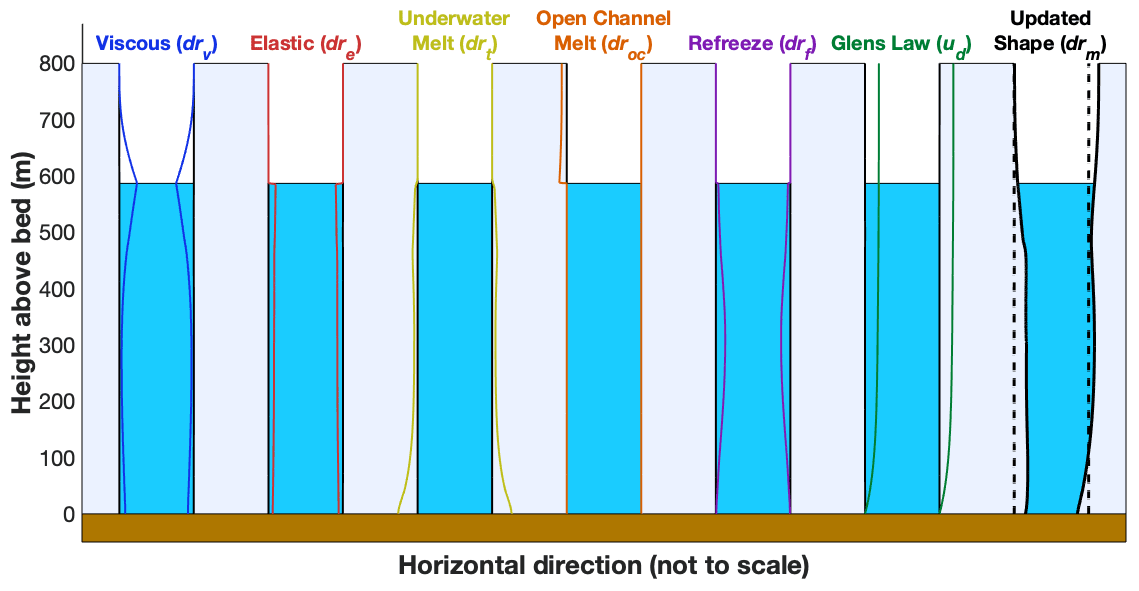
Figure 1 Processes included in the MouSh model. Black lines show a base moulin geometry that each process acts on, and colored lines show the change in moulin geometry (not to scale) due to that process alone. From left to right: changes in moulin geometry due to viscous deformation, elastic deformation, melting by turbulent energy dissipation of flowing water inside the moulin, melting by open-channel water flow, refreezing over winter inside the moulin, and deformation due to ice motion prescribed by Glen's flow law. Unlike the other components, elastic deformation is instantaneous but applied over the model time step (Sect. 2.2.1; Supplement Sect. S1). The right-most moulin shows the moulin geometry before (dashed black lines) and after (solid black lines and blue water) several hypothetical model time steps, i.e., the sum of all processes shown in the preceding panels. Changes are not to scale.

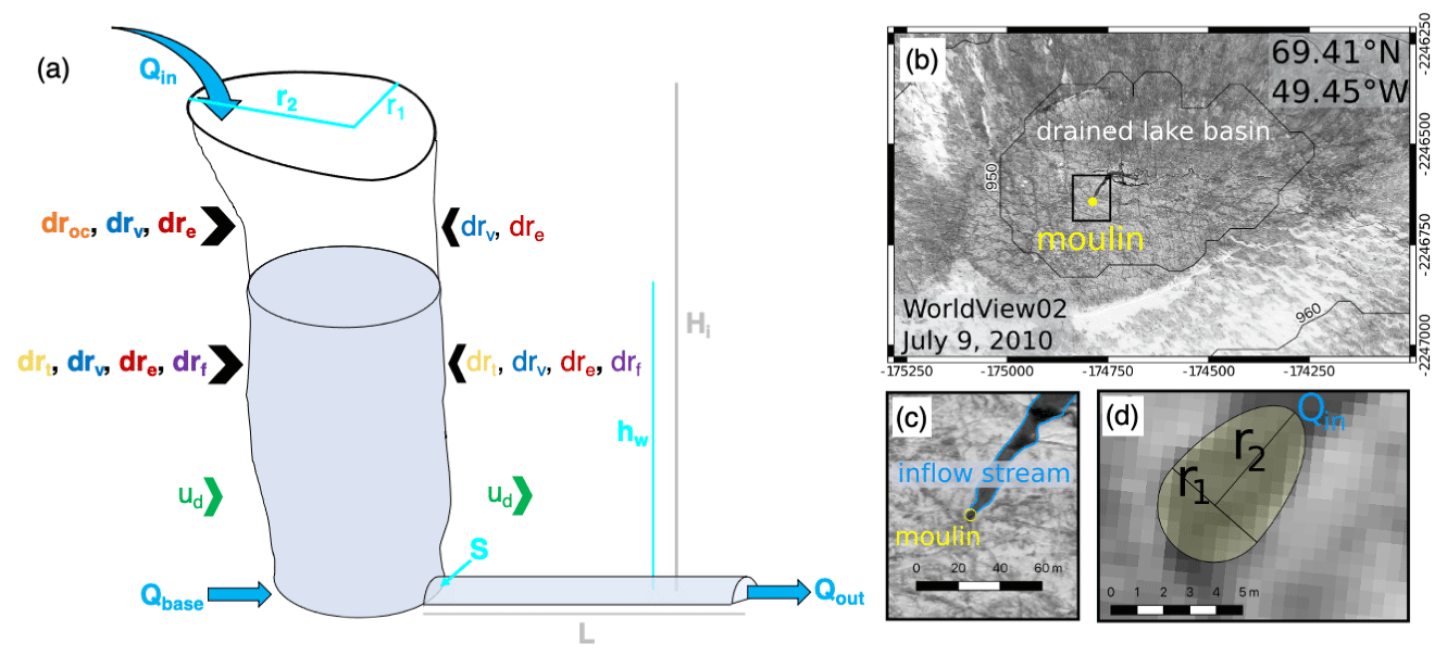
Figure 2 MouSh geometry and surface expression of a moulin and its reflection in the MouSh model. (a) Schematic of MouSh geometry and inputs. Inflow and outflow of the system are indicated by Q_in, Q_out, and Q_base. Time-evolving moulin and subglacial parameters include moulin radii (r₁,r₂), moulin water level (h_w), and subglacial cross-sectional area (S). r₁ and r₂ are evolved by dr_oc, dr_v, dr_e, dr_f, and dr_t (open-channel melting, viscous deformation, elastic deformation, refreezing, and turbulent melting, respectively; colored as in Fig. 1). u_d shears the moulin as prescribed by Glen's flow law. Ice thickness and subglacial path length are indicated by H_i and L, respectively. Ice flow is from left to right. Modified from Trunz (2021). (b) WorldView-2 scene from July 2010 of an approximately 1.2 km ×0.8 km region surrounding the example moulin (yellow) formed by a drained supraglacial lake. (c) Detail of panel (b), with the inflow stream and moulin indicated. (d) Detail of panel (c), showing the moulin minor radius r₁, major radius r₂, and water input Q_in from the inflow stream, as represented in the MouSh model. Maps generated by authors. WorldView image © 2010 DigitalGlobe, Inc.

2.1 Moulin geometry coordinate system

We discretize our model in the vertical (z) and radial (r₁ and r₂, or generally r_m) directions, treating the moulin as a stack of egg-shaped (semi-circular, semi-elliptical) holes in the ice that both change in size and move laterally relative to each other. We calculate moulin geometry (elliptical radii r₁ and r₂) and water level h_w with a 5 min time step dt. Model calculations are performed in cylindrical coordinates, where Π(z) is the perimeter of the semi-circular, semi-elliptical moulin, using Ramanujan's approximation:

$$\begin{array}{}\text{(1)}& \mathrm{\Pi }\approx \mathit{\pi }{r}_{\mathrm{1}}+{\displaystyle \frac{\mathrm{1}}{\mathrm{2}}}\mathit{\pi }\left[\mathrm{3}\right(r_{\mathrm{1}}+r_{\mathrm{2}})-\sqrt{(\mathrm{3}{r}_{\mathrm{1}}+r_{\mathrm{2}})(r_{\mathrm{1}}+\mathrm{3}{r}_{\mathrm{2}})}].\end{array}$$

Here, r₁ and r₂ are the minor and major radii, respectively, for each node in the vertical direction. The minor radius r₁ is also the radius of the half-circle.

We calculate the cross-sectional area A_m of the semi-circular, semi-elliptical moulin as follows:

$$\begin{array}{}\text{(2)}& A_{\mathrm{m}}={\displaystyle \frac{\mathit{\pi }{r}_{\mathrm{1}}}{\mathrm{2}}}(r_{\mathrm{2}}+r_{\mathrm{1}}).\end{array}$$

The plan-view orientation of the radii and the coordinate system, as detailed on a remotely sensed moulin, are indicated in Fig. 2b–d. The elliptical shape was chosen to reflect the observation that supraglacial meltwater flows into a moulin along a single side above the water line. This asymmetry leads to a nonuniform, noncircular geometry above the water level. This choice is in line with observations of a GrIS moulin becoming more elliptical over time (Röösli et al., 2016). For simplicity, MouSh also contains an option to set the moulin cross-sectional geometry to a circle, rather than an egg (see Supplement Sect. S2.2.2).

Each module is also dependent on the depth-varying hydrostatic and cryostatic pressures. We subtract the cryostatic pressure P_i from the hydrostatic pressure P_w to calculate the total depth-dependent pressure P at all vertical levels z within the moulin:

$$\begin{array}{}\text{(3a)}& {\displaystyle }{P}_{\mathrm{i}}={\mathit{\rho }}_{\mathrm{i}}g(H_{\mathrm{i}}-z),\text{(3b)}& {\displaystyle }{P}_{\mathrm{w}}={\mathit{\rho }}_{\mathrm{w}}g(h_{\mathrm{w}}-z),\text{(3c)}& {\displaystyle }P=P_{\mathrm{w}}-P_{\mathrm{i}},\end{array}$$

where H_i is the ice thickness; h_w is the height of the water above the bed (moulin water level); z is the vertical coordinate; ρ_i and ρ_w are ice and water density, respectively; and g is gravitational acceleration (Table 1). Note that P is not effective pressure, which is defined as $P=P_{\mathrm{i}}-P_{\mathrm{w}}$ (Cuffey and Paterson, 2010). In our formulation, positive pressures cause outward expansion of the moulin walls (radial growth), and negative pressures reduce the size of the moulin (radial closure). We use a flat bed at sea level for all model runs presented here; bed elevation is $z=b=\mathrm{0}$.

Table 1 MouSh model constants and parameter ranges. During realistic runs (Sect. 2.5.3) Values used during realistic model experiments are generally the median value of the sensitivity experiment.

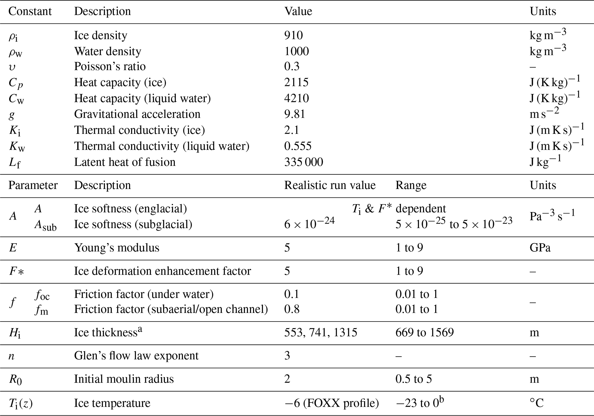
^a H_i defines distance from terminus L and surface slope α based on a perfectly plastic ice surface profile. ^b Including Iken et al. (1993), Lüthi et al. (2015), and Ryser et al. (2014).

2.2 Ice deformation modules

We represent the deformation of the ice with the simplest possible combination of elastic and viscous components: a Maxwell rheology, where elastic and viscous deformation occur independently, without interaction (Turcotte and Schubert, 2002). The Maxwell model comprises an elastic element (a spring) and a viscous element (a dashpot) in series and is standard in geophysical modeling. The response timescale in our Maxwell model is equal to ($E\times A\times {\mathit{\tau }}^{\mathrm{2}}{)}^{-\mathrm{1}}$ where E is Young's modulus, A is the viscous flow law parameter, and τ is stress (Table 1; Turcotte and Schubert, 2002). The Maxwell timescale is thus roughly 10–100 h for typical Greenland ice.

Elastic deformation is described in Sect. 2.2.1. We represent total viscous deformation in two modes: (1) radial opening and closure of the moulin, which changes the size of the moulin (Sect. 2.2.2), and (2) vertical shear of the moulin, which changes the shape but not the size of the moulin (Sect. 2.2.3).

2.2.1 Elastic deformation

Field measurements indicate that, nearly universally during the melt season, the water level in a moulin varies at a sub-hourly timescale (Andrews et al., 2014; Covington et al., 2020; Cowton et al., 2013; Iken, 1972). This variability is shorter than, but comparable to, the Maxwell timescale for ice (10–100 h); therefore, we must assume that elastic deformation plays a role in the response of the ice to variations in moulin water level.

Weertman (1971, 1973, 1996) applied dislocation fracture mechanics principles to vertical glaciological features: water-filled crevasses. These equations have applied to supraglacial lake drainages (Krawczynski et al., 2009) and slow ice hydrofracture (Poinar et al., 2017). However, these problems are Cartesian (linear), not cylindrical, so their solutions are not readily adaptable to a moulin. The stress and deformational patterns around cylindrical boreholes have been well studied in the rock mechanics literature (Amadei, 1983; Goodman, 1989; Priest, 1993). We therefore base our description of the stress field surrounding the moulin on that of a fluid-filled borehole in a porous rock medium, described by Aadnøy (1987) and based on the Kirsch equations, which describe stresses surrounding a circular hole in a rigid plate (Kirsch, 1898). We assume plane strain and approximate our moulin as a stack of such plates with analogous holes (Goodman, 1989). A subtle difference is that our moulin shape is not circular, but egg-shaped: half circular, half elliptical.

At each vertical level z in the moulin, we apply Hooke's law to the stress field to calculate the strain, in horizontal cross section, at all points on the moulin wall and in the surrounding ice for both radii r₁ and r₂. We then integrate these strains from an infinite distance (cylindrical coordinate r=∞) to the moulin wall (r_m). A full derivation, based on the stress states in a borehole described by Aadnøy (1987), is in Supplement Sect. S1. We express the total radial elastic deformation r_e of a moulin segment as

$$\begin{array}{}\text{(4)}& \begin{array}{rl}{r}_{\mathrm{e}}& ={\displaystyle \frac{r_{\mathrm{m}}}{E}}\left[\right(\mathrm{1}+\mathit{\nu }\left)\right(\mathrm{\Delta }P-{\displaystyle \frac{\mathrm{1}}{\mathrm{2}}}(\mathrm{\Delta }{\mathit{\sigma }}_x+\mathrm{\Delta }{\mathit{\sigma }}_y)\\ & +{\displaystyle \frac{\mathrm{1}}{\mathrm{4}}}(\mathrm{\Delta }{\mathit{\sigma }}_x-\mathrm{\Delta }{\mathit{\sigma }}_y)(\mathrm{1}-\mathrm{3}\mathit{\nu }-\mathrm{4}{\mathit{\nu }}^{\mathrm{2}})\\ & +{\displaystyle \frac{\mathrm{1}}{\mathrm{4}}}\mathrm{\Delta }{\mathit{\tau }}_{xy}(\mathrm{2}-\mathrm{3}\mathit{\nu }-\mathrm{8}{\mathit{\nu }}^{\mathrm{2}})].\end{array}\end{array}$$

Here, ΔP is the change in cryo-hydrostatic pressure (Eq. 3c) over a time interval; ν is Poisson's ratio; r_m is used to refer to r₁ or r₂; and Δσ_x, Δσ_y, and Δτ_xy are changes in background deviatoric and shear stresses that describe the regional setting of the moulin. The model is designed to accept user-defined deviatoric and shear stresses; however, we choose a neutral surface stress state ($\mathrm{\Delta }{\mathit{\sigma }}_x=\mathrm{\Delta }{\mathit{\sigma }}_y=\mathrm{\Delta }{\mathit{\tau }}_{xy}$ 0 kPa) for experimental simplicity and because these stresses and their changes over time are poorly constrained. This simplification reduces elastic deformation r_e:

$$\begin{array}{}\text{(5)}& r_{\mathrm{e}}={\displaystyle \frac{r_{\mathrm{m}}}{E}}(\mathrm{1}+\mathit{\nu })\mathrm{\Delta }P.\end{array}$$

Unlike viscous deformation and melting, elastic deformation is instantaneous. However, we take advantage of the observation that elastic deformation is driven by changes in the cryostatic and hydrostatic pressures (Supplement Sect. S1.5).

Therefore, we express Eqs. (4) and (5) as an elastic “deformation rate” for varying (Eq. 6) and constant (Eq. 7) surface stresses.

$$\begin{array}{}\text{(6)}& {\displaystyle }\begin{array}{rl}{\displaystyle \frac{\mathrm{d}{r}_{\mathrm{e}}}{\mathrm{d}t}}& ={\displaystyle \frac{\mathrm{1}}{E}}\left(r_{\mathrm{m}}(\mathrm{1}+\mathit{\nu }){\displaystyle \frac{\mathrm{d}P}{\mathrm{d}t}}+\left[(\mathrm{1}+\mathit{\nu })\left(-{\displaystyle \frac{\mathrm{1}}{\mathrm{2}}}\left({\displaystyle \frac{\mathrm{d}{\mathit{\sigma }}_x}{\mathrm{d}t}}+{\displaystyle \frac{\mathrm{d}{\mathit{\sigma }}_y}{\mathrm{d}t}}\right)\right.\right.\right.\\ & +{\displaystyle \frac{\mathrm{1}}{\mathrm{4}}}\left({\displaystyle \frac{\mathrm{d}{\mathit{\sigma }}_x}{\mathrm{d}t}}-{\displaystyle \frac{\mathrm{d}{\mathit{\sigma }}_y}{\mathrm{d}t}}\right)(\mathrm{1}-\mathrm{3}\mathit{\nu }-\mathrm{4}{\mathit{\nu }}^{\mathrm{2}})\\ & \left.\left.+{\displaystyle \frac{\mathrm{1}}{\mathrm{4}}}{\displaystyle \frac{\mathrm{d}{\mathit{\tau }}_{xy}}{\mathrm{d}t}}(\mathrm{2}-\mathrm{3}\mathit{\nu }-\mathrm{8}{\mathit{\nu }}^{\mathrm{2}})\right]\right)\end{array}\text{(7)}& {\displaystyle }\mathrm{d}{r}_{\mathrm{e}}={\displaystyle \frac{r_{\mathrm{m}}}{E}}(\mathrm{1}+\mathit{\nu })\left({\displaystyle \frac{\mathrm{d}P}{\mathrm{d}t}}\right)\mathrm{d}t\end{array}$$

Equations (6) and (7) assume that both effective pressure and moulin radius vary smoothly over the time interval in question, which is generally true for small time steps (5 min in our model). The dominant term in Eq. (6) is the first term, since $\frac{\mathrm{d}P}{\mathrm{d}t}$ (∼1 kPa over a typical hour during the melt season) greatly exceeds the rate of change of the surface stresses (∼1 kPa over a year), as explained in the Supplement Sect. S1. Equation (7) is commonly used for dilatometer testing in rock mechanics (Goodman, 1989).

2.2.2 Viscous radial opening and closure

Moulins close when they lose their water source at the end of a melt season (Catania and Neumann, 2010). Similarly, boreholes close if they are not filled with drilling fluid with a density like ice (Alley, 1992). Our modeled moulin is intermediate to these edge cases because it typically contains water. When the moulin is filled with water to the flotation level, it will stay open at its base and viscously close at and below the water level. The moulin will viscously open in regions where hydrostatic pressure exceeds the cryostatic pressure. When the water level is below flotation, which is the typical case, viscous deformation shrinks the moulin at all depths.

We calculate strain rate $\dot{\mathit{\epsilon }}$ from the total depth-dependent pressure P (Eq. 3c) using Glen's flow law:

$$\begin{array}{}\text{(8)}& \dot{\mathit{\epsilon }}=F^{\ast }A\left(T_{\mathrm{i}}{P}_{\mathrm{i}}\right)\cdot {\left({\displaystyle \frac{\mathrm{1}}{\mathrm{3}}}P\right)}^n,\end{array}$$

where F^∗ is the flow law enhancement factor, A(T_i,P_i) is the flow law parameter, and n is Glen's flow law exponent. For the flow law parameter, we use the standard relationship from Cuffey and Paterson (2010, Eq. 3.35), which is a function of ice temperature T_i and ice pressure P_i.

We follow borehole studies by Naruse et al. (1988) and Paterson (1977) to write strain, ε, in the radial direction as

$$\begin{array}{}\text{(9)}& \mathit{\epsilon }=\ln \left({\displaystyle \frac{r_{\mathrm{f}}}{r_{\mathrm{0}}}}\right),\end{array}$$

where a moulin with initial radius r₀ and final radius r_f underwent radial strain of ε.

We use the time derivative of Eq. (9) to calculate the change in moulin radius due to viscous deformation:

$$\begin{array}{}\text{(10)}& \mathrm{d}{r}_{\mathrm{v}}=r_{\mathrm{m}}\exp \left(\dot{\mathit{\epsilon }}\mathrm{d}t\right)-r_{\mathrm{m}},\end{array}$$

with strain rate given by Eq. (8). This is the same relationship used by Catania and Neumann (2010).

2.2.3 Shear deformation

We use Glen's flow law to calculate the change in shape of the moulin due to regional-scale ice flow. This deforms the entire moulin in bulk, shearing it in the vertical and shifting it laterally downstream, without changing its radii. Basal sliding is not currently included in the model. To represent deformation, we discretize the moulin as a stack of plates with elliptical (or circular) holes with a thickness dz and represent deformational ice flow as displacement between these plates.

We calculate the rate of deformational ice flow u_d in the downstream direction from ice temperature T_i and pressure P_i, surface slope α, a constant F^∗, and H_i, using Glen's flow law (Cuffey and Paterson, 2010):

$$\begin{array}{}\text{(11)}& u_{\mathrm{d}}=\mathrm{2}F\cdot ({\mathit{\rho }}_{\mathrm{i}}g\mathit{\alpha }{)}^n\cdot \underset{b}{\overset{H_{\mathrm{i}}}{\int }}A(T_{\mathrm{i}},P_{\mathrm{i}}\left)\right(H_{\mathrm{i}}-z{)}^n\mathrm{d}z,\end{array}$$

where b is the ice sheet bed. We obtain ice deformation rates of ∼20 m yr⁻¹, which is typical of the ablation zone in western Greenland (Ryser et al., 2014).

2.3 Phase change modules

The second mode that changes the geometry of the moulin is ice ablation from or accretion to the moulin walls. During the melt season, the flow of water into and through the moulin generates turbulence, which as it dissipates acts to melt back the moulin walls, expanding the size of the moulin. There is also a small component of melting due to temperature differences between the water and surrounding ice. Outside the melt season, conduction of latent heat into the surrounding ice causes stagnant water to freeze back onto the moulin walls, contracting the size of the moulin.

2.3.1 Refreezing

Refreezing occurs in cold ice when water flow is absent or slow enough that the rate of heat conduction into the surrounding ice drops the water temperature to the freezing point. These conditions occur primarily outside the melt season. When these conditions are met, we apply a radial freezing r_f, which is parameterized economically, following Alley et al. (2005):

$$\begin{array}{}\text{(12)}& \mathrm{d}{r}_{\mathrm{f}}=\mathrm{2}{\displaystyle \frac{T_{\mathrm{i}}-T_{\mathrm{pmp}}}{L_{\mathrm{f}}}}\sqrt{{\displaystyle \frac{K_{\mathrm{i}}{C}_p}{\mathit{\pi }{\mathit{\rho }}_{\mathrm{i}}}}}\left(\sqrt{t_{\mathrm{t}}}-\sqrt{t_{\mathrm{t}}-\mathrm{d}t}\right).\end{array}$$

Here, T_i−T_pmp is the depth-varying difference between the far-field temperature (prescribed as from borehole temperature observations) and the moulin water temperature, which is taken as the pressure melting temperature T_pmp. L_f is the latent heat of fusion, K_i is water's thermal conductivity, and C_p is the specific heat capacity of ice. The refreezing rates evolve exclusively based on the elapsed time since the cessation of turbulent flow t_t.

We calculate the change in moulin water volume from freezing, V_frz, by summing the refrozen ice thickness in a time step, dr_f, around the perimeter of the moulin at all depths, z, and converting ice volume to water volume:

$$\begin{array}{}\text{(13)}& V_{\mathrm{frz}}={\displaystyle \frac{{\mathit{\rho }}_{\mathrm{i}}}{{\mathit{\rho }}_{\mathrm{w}}}}\underset{b}{\overset{h_{\mathrm{w}}}{\int }}\mathrm{\Pi }\left(z\right)r_{\mathrm{f}}\left(z\right)\mathrm{d}z.\end{array}$$

2.3.2 Moulin wall melting

During the melt season, turbulent energy dissipation from water flowing through the moulin melts back the moulin walls. We parameterize melting due to the dissipation of turbulent energy in two separate spatial domains: (1) within the water column of the moulin, where r₁ and r₂ are evolved uniformly, and (2) above the water level along the side of the moulin, as supraglacial input falls to the water level, where only r₂ is evolved.

The parameterizations of turbulently driven melting we use in both regimes rely on three simplifications. First, the volume of water moving through each vertical model node is constant within each time step. This ensures that water mass is conserved and that all model elements below the water line are water filled; however, this eliminates the potential long-term storage of meltwater within plunge pools caused by non-uniform incision into the ice. Second, all energy generated from turbulent dissipation is instantaneously applied to melting the surrounding ice. This neglects any heat transport within the water, which is a common approximation in subglacial models (e.g., Hewitt, 2013; Schoof, 2010; Werder et al., 2013). Third, we also make the simplifying assumption that meltwater entering the moulin is at 0 ^∘C and at the pressure melting temperature T_pmp at all points below the water line, although we do not model the impact of this temperature change on melting because moulin water temperatures are unknown.

Submerged zone. Below the water line, the vertical velocity of the water is dictated by the hydraulic gradient within the system and the local cross-sectional area of the moulin. Under such conditions, head loss – the departure of the hydraulic head from that calculated by Bernoulli's equation – reflects the energy dissipated as heat. We parameterize head loss using the Darcy–Weisbach equation, which relates water velocity u_w to changes in the hydraulic gradient $\mathrm{d}{h}_{\mathrm{w}}/\mathrm{d}l$ (head loss per unit length along flow), via the hydraulic radius R_h and a dimensionless friction factor f. Because water velocity is constrained by mass balance within the system, we calculate the head loss $\mathrm{d}{h}_{\mathrm{w}}/\mathrm{d}l$ as follows:

$$\begin{array}{}\text{(14)}& {\displaystyle \frac{\mathrm{d}{h}_{\mathrm{w}}}{\mathrm{d}l}}={\displaystyle \frac{u_{\mathrm{w}}^{\mathrm{2}}f}{\mathrm{8}{R}_{\mathrm{h}}g}}.\end{array}$$

The differential element dl represents the path length over which the water experiences head loss: $\mathrm{d}l=\sqrt{\mathrm{d}{x}^{\mathrm{2}}+\mathrm{d}{z}^{\mathrm{2}}}$ for horizontal distance dx and vertical drop dz. The friction factor f is a unitless model parameter that controls the rate of head loss within the system. Its value thus directly affects the amount of melting. Most subglacial models fix the Darcy–Weisbach friction factor, with values ranging from 0.01 to 0.5 (e.g., Colgan et al., 2011; Schoof, 2010; Spring and Hutter, 1981) or use equivalent values of Manning's n (e.g., Hewitt, 2013; Hoffman and Price, 2014). Alternatively, other models parameterize channel roughness using a geometry-dependent friction factor (e.g., Boulton et al., 2007; Clarke, 2003; Flowers, 2008). Thus, MouSh has options for fixed or variable f.

The friction factor within the submerged zone is indicated by f_m and in the open channel zone by f_oc. To explore the impact of the chosen friction factor, we complete a sensitivity study (Sects. 2.5.2 and 3.2). We use a constant f_m=0.1 for all other model runs presented.

Because we approximate the moulin as a half-circular, half-elliptical cylinder with perimeter Π, the hydraulic radius R_h of a water filled node is

$$\begin{array}{}\text{(15)}& R_{\mathrm{h}}={\displaystyle \frac{A_{\mathrm{m}}}{\mathrm{\Pi }}}.\end{array}$$

To calculate moulin wall melting, we use a simple energy balance equation, following previous work (e.g., Gulley et al., 2014; Jarosch and Gudmundsson, 2012; Nossokoff, 2013):

$$\begin{array}{}\text{(16)}& {\mathit{\rho }}_{\mathrm{i}}{C}_{\mathrm{w}}(T_{\mathrm{pmp}}-T_{\mathrm{i}}){\displaystyle \frac{\mathrm{d}{A}_{\mathrm{m}}}{\mathrm{d}t}}+{\mathit{\rho }}_{\mathrm{i}}{L}_{\mathrm{f}}{\displaystyle \frac{\mathrm{d}{A}_{\mathrm{m}}}{\mathrm{d}t}}=Q_{\mathrm{out}}\left({\mathit{\rho }}_{\mathrm{w}}g{\displaystyle \frac{\mathrm{d}{h}_{\mathrm{w}}}{\mathrm{d}l}}\right),\end{array}$$

where C_w is the heat capacity of water. The first term represents the energy needed to warm the surrounding ice to the pressure melting temperature of water T_pmp. Equation (16) can be rearranged and combined with Eq. (14) to provide the area of ice melted:

$$\begin{array}{}\text{(17)}& \mathrm{d}{A}_{\mathrm{t}}=Q_{\mathrm{out}}\left({\mathit{\rho }}_{\mathrm{w}}g{\displaystyle \frac{u_{\mathrm{w}}^{\mathrm{2}}f}{\mathrm{4}{R}_{\mathrm{h}}g}}\right){\left({\mathit{\rho }}_{\mathrm{i}}{C}_{\mathrm{w}}(T_{\mathrm{pmp}}-T_{\mathrm{i}})+{\mathit{\rho }}_{\mathrm{i}}{L}_{\mathrm{f}}\right)}^{-\mathrm{1}}\mathrm{d}t,\end{array}$$

where Q_out is the discharge from the moulin–subglacial system as dictated by the subglacial model component (Sect. 2.4.2), and T_pmp−T_i is the temperature difference between the water (prescribed to be at the pressure melting point) and the surrounding ice. We vary T_i based on observations as described in Table 1 and Sect. 2.5.2. Note that Eq. (17) determines the area of ice that is removed through melting. For each time step, we reframe Eq. (17) into radial melting within an egg-shaped moulin using information about the previous geometry and the assumption that melting occurs uniformly around the perimeter:

$$\begin{array}{}\text{(18)}& \mathrm{d}{r}_{\mathrm{t}}=\mathrm{2}\mathrm{d}{A}_{\mathrm{t}}/\left[\mathit{\pi }(\mathrm{5}{r}_{\mathrm{1}}+\mathrm{3}{r}_{\mathrm{2}}-\sqrt{(\mathrm{3}{r}_{\mathrm{1}}+r_{\mathrm{2}})(r_{\mathrm{1}}+\mathrm{3}{r}_{\mathrm{2}})})\right].\end{array}$$

Equation (18) is simplified when considering a circular geometry (r₁=r₂).

Unsubmerged zone. Above the water line, a variety of complex processes drive melting. A first-principles approach would be to quantify melting due to the potential energy loss of falling water, following the work on terrestrial waterfalls (e.g., Scheingross and Lamb, 2017). However, nearly all waterfall parameterizations rely on abrasion between waterborne sediment and the substrate as the primary mechanism of erosion. Instead, we implement a simple parameterization for open-channel flow with the understanding that the complexities of thermal erosion are not completely captured. In our model, open-channel melting occurs only on the up-glacier wall of the moulin and follows two ad hoc rules based on the slope between the vertical nodes: (1) open-channel turbulent melting is applied if the slope of the upstream moulin wall allows water to flow over it, and (2) a small prescribed amount of melting is applied when the upstream wall slope is vertical or overhung, because while water cannot flow directly along the ice, spray and other processes likely drive some amount of melting. These cases are respectively (1) the open-channel zone and (2) the falling-water zone.

In the open-channel zone, we use a similar approach as for melting below the water line. However, the hydraulic radius R_h is adjusted to reflect the observation that water runs down only one wall of the moulin, and a higher friction factor is used to parameterize complex geometries. Due to the presence of a discontinuity between open-channel and water-filled regions (at the water line), we parameterize the hydraulic radius of open channel flow as $R_{{\mathrm{h}}_{\mathrm{open}}}=\mathrm{0.5}{r}_{\mathrm{2}}$. We also use a higher open channel friction factor f_oc of 0.8 to parameterize observed extensive scalloping (e.g., Gulley et al., 2014; Covington et al., 2020). We apply melting to only the elliptical side of the moulin, defined by r₂ using Eq. (18). Note that the hydraulic radius prescribed for open-channel flow is likely larger than the small region over which water is flowing in the natural system (Fig. 2). Further, the resulting open channel melt dA_oc is applied only to the major radius to calculate the change in open channel radius dr_oc.

In the falling-water zone, there is very limited interaction between the moulin walls and the water. For simplicity, we assume that a small fraction, f_p, of the potential energy lost as water falls is deposited into the moulin walls, perhaps as the kinetic energy of spray. The change in radius due to this process is as follows:

$$\begin{array}{}\text{(19)}& \mathrm{d}{r}_{\mathrm{mf}}=f_{\mathrm{p}}{\displaystyle \frac{({\mathit{\rho }}_{\mathrm{w}}/{\mathit{\rho }}_{\mathrm{i}})g{Q}_{\mathrm{out}}}{L_{\mathrm{f}}\mathrm{\Pi }}}\mathrm{d}t.\end{array}$$

We set f_p to 0.1 for all model runs presented here.

We add the volume of ice melted to the water already in the moulin, similarly to Eq. (12) for V_frz. We calculate the change in moulin water volume from melting by summing the melted ice thickness, r_mf, around the perimeter of the moulin at all depths z and converting ice volume to water volume:

$$\begin{array}{}\text{(20)}& V_{\mathrm{wallmelt}}={\displaystyle \frac{{\mathit{\rho }}_{\mathrm{i}}}{{\mathit{\rho }}_{\mathrm{w}}}}\mathrm{d}t\underset{b}{\overset{H_{\mathrm{i}}}{\int }}\left(\mathrm{\Pi }\right(z\left)\mathrm{d}{r}_{\mathrm{mf}}\right(z)+A_{\mathrm{oc}}(z)+A_{\mathrm{t}}(z\left)\right)\mathrm{d}z.\end{array}$$

2.4 Water flux into and out of the moulin (mass conservation)

Water balance within the moulin and the subglacial channel is dictated by recharge from a supraglacial stream (Q_in described below), discharge through a subglacial channel (Q_out, Q_base; described below), and any change in volume due to melting or refreezing, such that the volume of water in the system (V) is

$$\begin{array}{}\text{(21)}& {\displaystyle \frac{\mathrm{d}V}{\mathrm{d}t}}=Q_{\mathrm{in}}-Q_{\mathrm{out}}+Q_{\mathrm{base}}+{\displaystyle \frac{(\mathrm{d}{V}_{\mathrm{wallmelt}}-\mathrm{d}{V}_{\mathrm{frz}})}{\mathrm{d}t}}.\end{array}$$

The final term varies in space and time, with high rates of volume lost to melt above the water line during the melt season (when Q_in>0) and moderate rates of volume lost to melt at and below the water line during and after the melt season, when there is water flow through the moulin (Q_out>0), and refreezing below the water line throughout the winter (when $Q_{\mathrm{in}}=Q_{\mathrm{out}}=\mathrm{0}$). The MouSh model can also accept an additional prescribed baseflow Q_base directly to the subglacial module. We design baseflow as a loose approximation of additional subglacial water inputs from varied upstream sources, including other moulins on the same subglacial channel, regional basal melt, and the addition and removal of meltwater from subglacial storage. Baseflow is generally required to maintain realistic moulin water levels. In the moulin runs forced by realistic Q_in, we represent subglacial flow from about five surrounding moulins by prescribing baseflow as 5 times the running 5 d mean of Q_in. In other model runs, we do not include baseflow. The addition of baseflow is designed to represent the widespread seasonal evolution of surface melt; its inclusion maintains a slightly larger subglacial channel than would otherwise occur, which reduces otherwise unrealistically large daily swings in modeled moulin water level (Supplement Sect. S2.2.5).

2.4.1 Meltwater runoff from the ice sheet surface

We force the MouSh model with time-varying water inputs from the supraglacial environment, Q_in. We use two different Q_in scenarios: a simple diurnal cosine with a mean discharge of 5 m³ s⁻¹, in rough agreement with observations near the margins of the GrIS (Eq. 22, Chandler et al., 2013; McGrath et al., 2011; Smith et al., 2017), and realistic supraglacial discharge over a melt season, determined by using in situ surface melting data and internally drained catchment size and geometry (Yang and Smith, 2016).

We use the following cosine curve to represent our simplest form of supraglacial discharge into the moulin during sensitivity studies:

$$\begin{array}{}\text{(22)}& Q_{\mathrm{in}}=\cos \left(\mathit{\pi }\right(t-\mathrm{19.5})/\mathrm{12})+\mathrm{5}.\end{array}$$

Here, t is time in hours and Q_in is in m³ s⁻¹. This function has its daily peak at 19:30 UTC and a daily minimum at 07:30 UTC (Smith et al., 2021).

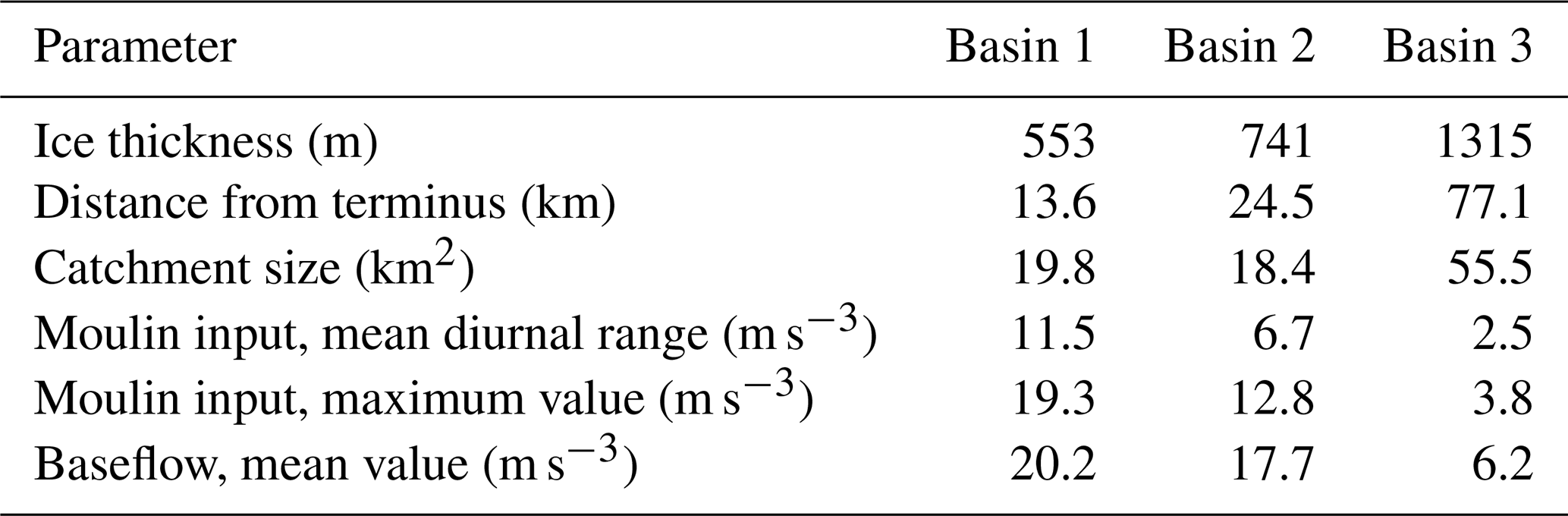
To examine a set of realistic moulins, we select three supraglacial basins from Yang and Smith (2016) and extract their size and distance from terminus from information provided therein (Basin 1–3; Table 2). We derive surface runoff from MERRA-2 reanalysis (Gelaro et al., 2017; Smith et al., 2017). Further details on supraglacial input characteristics are included in Sect. 2.5.3.

Table 2 General ice and moulin input parameters for realistic runs.

2.4.2 Water flow from the subglacial system

We couple the moulin model and a single evolving subglacial channel controlled by melt opening and creep closure (Covington et al., 2020; Schoof, 2010) using a reservoir-constriction model (Covington et al., 2012) that simulates flows between the moulin and subglacial channel. Following Covington et al. (2020), the rate of change of moulin water level h_w is

$$\begin{array}{}\text{(23)}& \mathrm{d}{h}_{\mathrm{w}}={\displaystyle \frac{\mathrm{1}}{A_{\mathrm{m}}\left(h_{\mathrm{w}}\right)}}\mathrm{d}V,\end{array}$$

with the change in water volume within the system being dV, and the volume of the moulin–subglacial system is related to the channel S and the moulin cross-sectional area A_m. The water volume is related to Q_in, Q_base, and Q_out, where Q_out is the meltwater output from the subglacial channel, defined as follows:

$$\begin{array}{}\text{(24)}& Q_{\mathrm{out}}=c_{\mathrm{3}}{S}^{\mathrm{5}/\mathrm{4}}\mathrm{\Psi }/\sqrt{\mathrm{|}\mathrm{\Psi }\mathrm{|}}.\end{array}$$

The hydraulic gradient $\mathrm{\Psi }=-{\mathit{\rho }}_{\mathrm{i}}g\frac{\mathrm{d}(h_{\mathrm{w}}-b)}{\mathrm{d}L}$ is a linear gradient in h_w to the outlet at a horizontal distance L, where the pressure head is zero. In our calculations, the bed elevation b is zero. Finally, c₃ is a flux parameter:

$$\begin{array}{}\text{(25)}& c_{\mathrm{3}}={\displaystyle \frac{{\mathrm{2}}^{\mathrm{5}/\mathrm{4}}}{{\mathit{\pi }}^{\mathrm{1}/\mathrm{4}}}}\sqrt{{\displaystyle \frac{\mathit{\pi }}{(\mathit{\pi }+\mathrm{2}){\mathit{\rho }}_{\mathrm{w}}{f}_{\mathrm{sub}}}}}.\end{array}$$

Equation (25) follows Covington et al. (2020), who corrected a small error from the original Schoof (2010) formulation.

We use an equation from Schoof (2010) for the time rate of change in subglacial channel cross-section area S, with the first part describing the turbulent melting of the subglacial channel walls and the second term describing closure due to the pressure of the overlying ice, which is dependent on effective pressure $N=P_{\mathrm{i}}-P_{\mathrm{w}}$:

$$\begin{array}{}\text{(26)}& \mathrm{d}S=(c_{\mathrm{1}}{Q}_{\mathrm{out}}\mathrm{\Psi }-c_{\mathrm{2}}{N}^{n}S)\mathrm{d}t.\end{array}$$

Here, the constant $c_{\mathrm{1}}=\frac{\mathrm{1}}{{\mathit{\rho }}_{\mathrm{i}}{L}_{\mathrm{f}}}$ and the constant $c_{\mathrm{2}}=\mathrm{2}{A}_{\mathrm{sub}}{n}^{-n}$ with Glen's flow law parameters for the subglacial component defined as $A_{\mathrm{sub}}=\mathrm{6}\times {\mathrm{10}}^{-\mathrm{24}}$ Pa⁻³ s⁻¹.

Replacing Q_out, Ψ, and N in Eq. (26) yields

$$\begin{array}{}\text{(27)}& \mathrm{d}S=c{(}_{\mathrm{1}}{c}_{\mathrm{3}}{S}^{\mathrm{5}/\mathrm{4}}{\left({\displaystyle \frac{{\mathit{\rho }}_{\mathrm{w}}g{h}_{\mathrm{w}}}{L}}\right)}^{\mathrm{3}/\mathrm{2}}-c_{\mathrm{2}}(P_{\mathrm{i}}-{\mathit{\rho }}_{\mathrm{w}}g{h}_{\mathrm{w}}{)}^{n}S)\mathrm{d}t.\end{array}$$

Equations (23) and (27) are numerically solved simultaneously, as in Schoof (2010) and Covington et al. (2020). The parameters used in the subglacial module are included in Table 1 and are the same as those used in the englacial component of MouSh, apart from the flow law parameter A_sub. In the englacial system, A is calculated from local temperature within the ice column, which can be as cold as −23 ^∘C in western Greenland (Iken et al., 1993). This contrasts with the temperature at the ice–bed interface, which must be at the melting point; the subglacial component of MouSh uses a fixed A_sub value.

In its current configuration, the subglacial module provides a single set of outputs representative of conditions at the moulin. This is primarily because this study focuses on the evolution of a moulin and is not representative of a channel running from a moulin to the terminus in a natural system. A more complex subglacial model would more accurately resolve the spatial changes in subglacial channel geometry and flow.

2.5 Suites of model experiments

To examine the sensitivity of the MouSh model to uncertain parameters, ice and meltwater characteristics, and model choices and difference from previous moulin parameterizations, we completed four suites of experiments. While these experiments do not cover the complete range of possibilities, they were designed to address primary uncertainties in the MouSh model and examine how moulin geometry might vary spatially and temporally.

2.5.1 Sensitivity diurnal supraglacial variability

Under steadily varying conditions such as a repeating diurnal variation, the modeled moulin reaches a quasi-equilibrium state independent of initial conditions with melting opposing viscous and elastic deformation and the only change being driven by shear deformation. Moulin water level and shape respond to these patterns of variability. To examine the impact of Q_in magnitude (mean) and Q_in amplitude (variability), we perform a series of model runs that vary the magnitude of a cosine curve between 1 and 20 m³ s⁻¹ with a fixed amplitude of 0.5 m³ s⁻¹ and a series of runs that vary the amplitude of a cosine curve between 0 and 2 m³ s⁻¹ with a fixed magnitude of 5.0 m³ s⁻¹. The amplitude is one-half the diurnal range. These runs use Basin 1 ice conditions (Table 2; Sect. 2.5.3). Further details can be found in Supplement Sect. S2.1 and Figs. S2–S4.

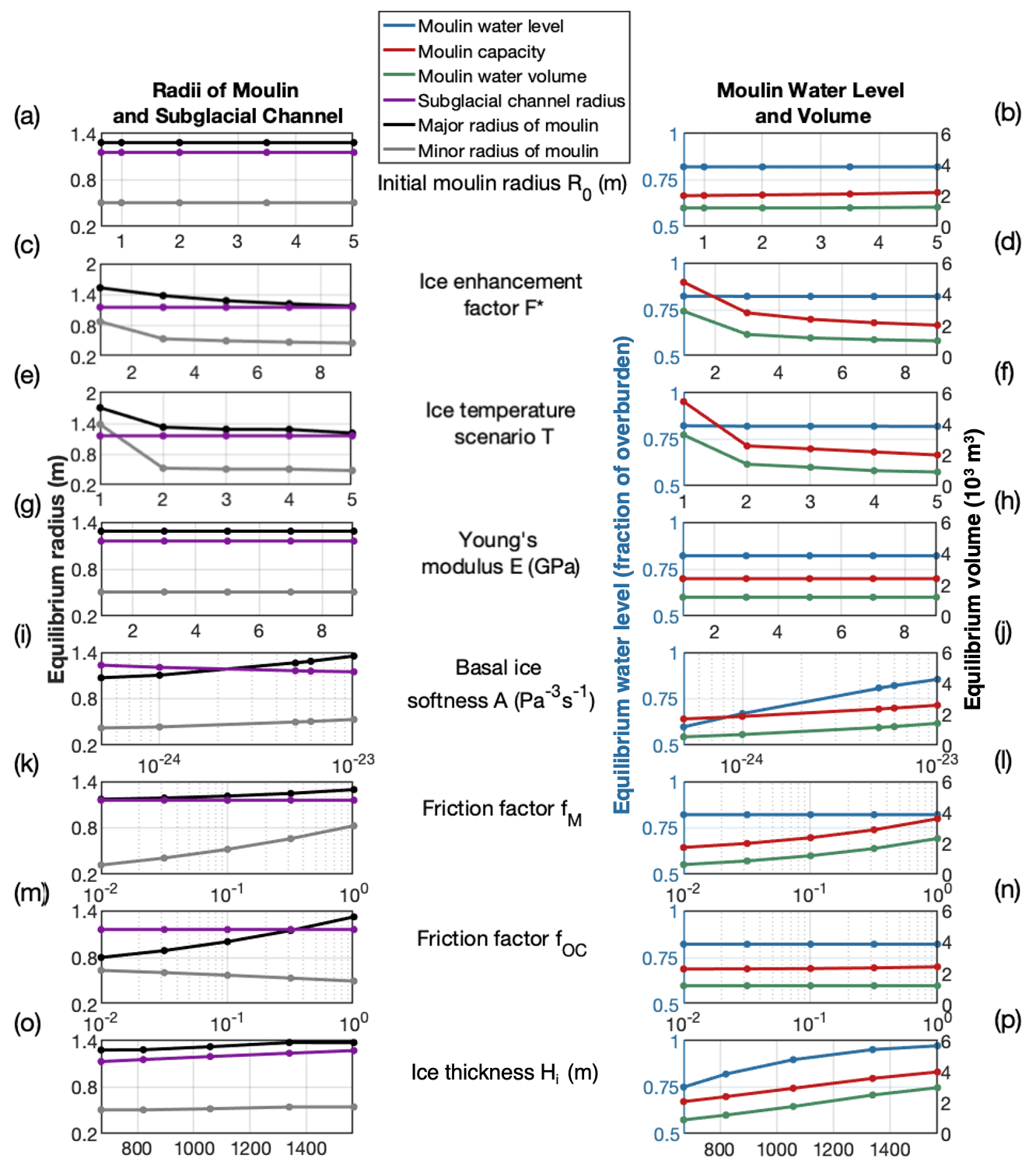
Figure 3 Results of parameter sensitivity studies for 40 d MouSh model runs. Shown are the sensitivity of moulin size to initial condition for moulin radius (a, b), enhancement factor for englacial ice (c, d), ice temperature scenario (e, f), Young's modulus (g, h), softness of basal ice (i, j), friction factor for water flow beneath the water line (k, l), friction factor for water flow above the water line (m, n), and ice thickness (o, p). The left column shows the moulin radii (black and grey) at the mean water level and the mean subglacial channel radius (purple) averaged over the final 24 h period of the 40 d model run. The right column shows the equilibrium water level (blue), moulin capacity (red), and volume of water in the moulin (green) averaged over the same 24 h period. Overall, moulin radius is most sensitive to the friction factors, while moulin water level and volume are most sensitive to ice thickness (also an indicator of the hydraulic potential gradient) and basal ice softness. Note the different y-axis range in panels (c) and (e).

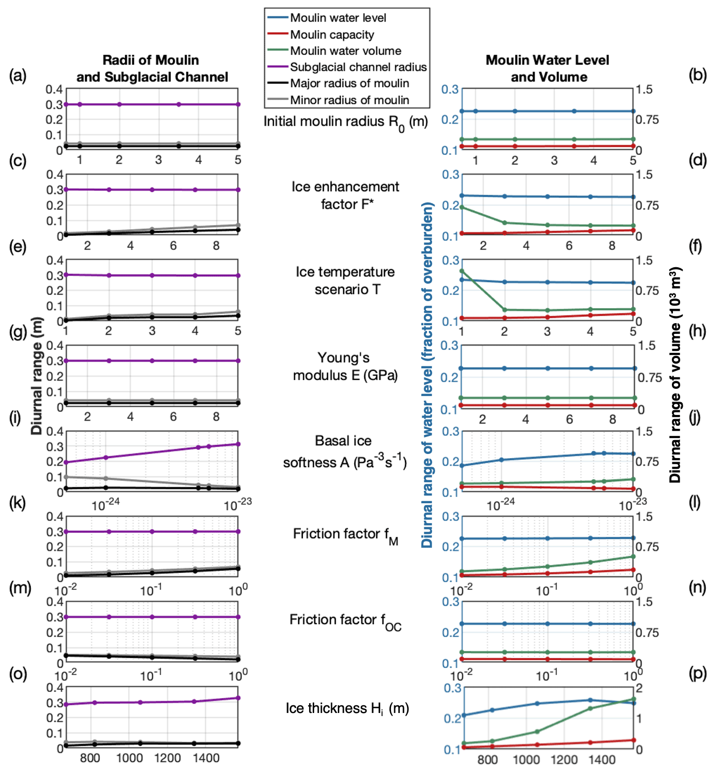
Figure 4 Diurnal variations in moulin sizes in 40 d parameter sensitivity runs. Shown are the sensitivity of diurnal variation in moulin size and water storage metrics to initial condition for moulin radius (a, b), enhancement factor for englacial ice (c, d), ice temperature scenario from coldest to warmest ice (e, f), Young's modulus (g, h), softness of basal ice (i, j), friction factor for water flow beneath the water line (k, l), friction factor for water flow above the water line (m, n), and ice thickness (o, p). The left column shows diurnal variations in moulin radii (black and grey) at the equilibrium water level and the subglacial channel radius (purple) in the final 24 h period of the 40 d model run. The right column shows the diurnal variation in water level (blue), moulin capacity (red), and volume of water in the moulin (green) within the same 24 h period. Note the right y-axis difference in panel (p).

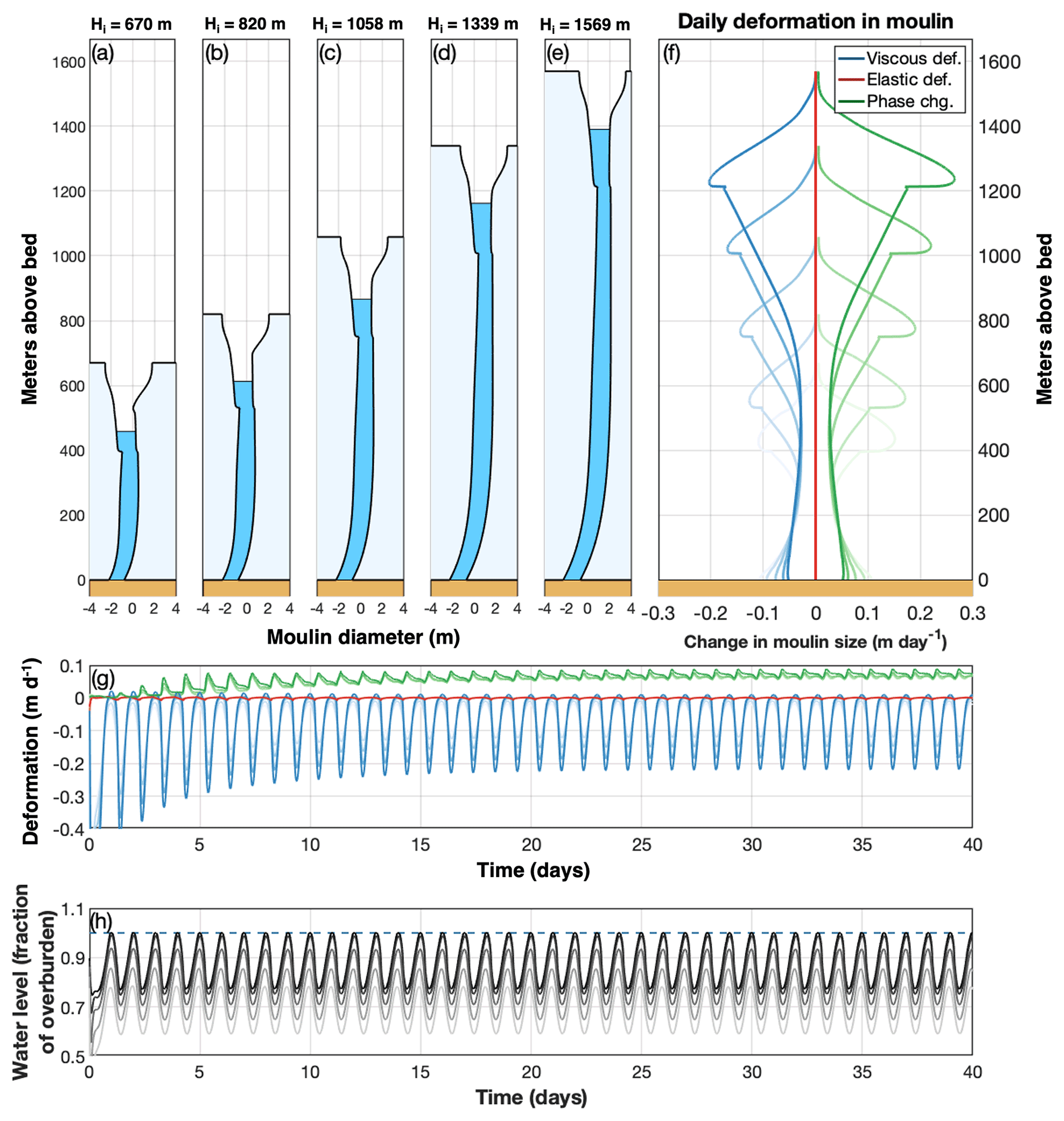
Figure 5 Contributions of viscous deformation, elastic deformation, and phase changes to moulin geometry. (a–e) Equilibrium geometries of five moulins in ice of different ice thicknesses H and different distances from the terminus (same as Fig. 6o and p) averaged over the final 24 h period of a 40 d model run. (f) Vertical variation in viscous deformation (blue), elastic deformation (red), and phase change (green) contributions to moulin geometry averaged over the same 24 h period. Negative values indicate contributions to moulin closure; positive values open the moulin. Darkening shades of each color map to moulins of increasing ice thickness. Closure and opening rates are greatest at the minimum daily water level (which is inferable by the lower notch in the moulin wall). (g) Time series of the components shown in panel (f) (colors the same) at the mean water level over the entire 40 d model run. The greater diurnal range in water level in moulins in thick ice drives the observed larger diurnal variations in viscous deformation. (h) For reference, moulin water level as a fraction of overburden for different ice thicknesses. Lighter greys indicate thinner ice; the blue dashed line indicates where fraction of overburden =1.

2.5.2 Sensitivity to uncertain parameters

We explored the sensitivity of our results to the values of seven parameters, shown in Figs. 3–5, with the prescribed ranges shown in Table 1. We examined the effect on the water level, the moulin radius at the equilibrium water level, the volume and water storage of the moulin, and the cross-sectional area of the subglacial channel at the end of a 40 d model run. These values reach equilibrium, with daily oscillations superimposed, after ∼15 d. We also tested the dependence of our results on the initial moulin radius, r₀, which we varied across an order of magnitude from 0.65 to 5.0 m.

We varied the value of a uniform deformation enhancement factor F^∗ over an order of magnitude ($F^{\ast }=\mathrm{1}$ to 9), which affects viscous flow of the ice surrounding the moulin. While the range of enhancement factors tested here cover a variety of ice conditions, including ice shelves and temperate glaciers, the GrIS likely has values between 4 and 6 (e.g., Cuffey and Paterson, 2010). Outside of testing the model sensitivity to the enhancement factor, we assigned $F^{\ast }=\mathrm{5}$. We also tested the effect of ice temperature, independent of the enhancement factor. We used five different temperature profiles: cold ice temperatures (mean $\sim -\mathrm{15}$ ^∘C, range −23.1 ^∘C to the pressure melting point) measured in the center of Jakobshavn Isbræ (Iken et al., 1993); moderate ice temperatures (mean $\sim -\mathrm{7}$ ^∘C, range −13.5 ^∘C to the pressure melting point) measured at the GULL site in Pâkitsoq (Lüthi et al., 2015; Ryser et al., 2014); warmer ice temperatures (mean $\sim -\mathrm{5}$ ^∘C, range −9.3 ^∘C to the pressure melting point) measured at the FOXX site in Pâkitsoq (Lüthi et al., 2015; Ryser et al., 2014); a hypothetical linear profile from −5 ^∘C at the surface to 0 ^∘C at the bed; and, finally, a fully temperate ice column. These different ice temperature scenarios affected the creep closure rates of ice through the temperature-dependent softness parameter A by approximately a factor of 6 from the coldest profile (Iken et al., 1993) compared to the fully temperate column.

We also examined moulin sensitivity to elastic deformation by varying Young's modulus (E) of the ice column between 1–9 GPa (Vaughan, 1995) and the sensitivity to the values of friction factors for the moulin walls. MouSh has two friction factors: f_m (below the water line) and f_oc (above the water line). We varied these friction factors across 2 orders of magnitude (0.01 to 1). We did not vary the subglacial channel friction factor. Finally, we varied values for basal ice softness A_sub over 2 orders of magnitude ($\mathrm{5}\times {\mathrm{10}}^{-\mathrm{25}}$ to $\mathrm{5}\times {\mathrm{10}}^{-\mathrm{23}}$) and independently examined moulins over a range of ice thicknesses (670–1570 m) and corresponding distance from the terminus (∼20–110 km), which in combination results in variations in hydraulic gradient.

2.5.3 Sensitivity to local conditions

We examined moulins over a range of ice thicknesses and corresponding distances from the terminus (Table 2). Each moulin is associated with a supraglacial basin derived by Yang and Smith (2016). The moulins were selected to be broadly representative of the range of ice thicknesses within the ablation zone of the western GrIS. These supraglacial drainage basin sizes and geometries are visually similar to nearby drainage basins and representative of the mean supraglacial drainage basin area for the given ice thicknesses. To derive broadly representative Q_in values for each basin, we integrate 3-hourly modeled surface melting from a downscaled version of MERRA-2 (Gelaro et al., 2017) over the surface area of each moulin surface drainage basin. We then use synthetic unit hydrograph parameters derived for a supraglacial basin from western Greenland during the middle of the 2019 melt season (Smith et al., 2017) to estimate supraglacial discharge into each moulin. Surface runoff values for the 2019 melt season were modified using a synthetic unit hydrograph derived for the ablation zone and parameters appropriate for the western GrIS (Smith et al., 2017) with manual dampening of diurnal variability to minimize long periods of no surface melt during the beginning and end of the season. We apply this dampening because the parameters for the unit hydrograph were determined during the middle of the melt season and therefore may inaccurately represent routing delays at the beginning and end of the melt season.

The supraglacial discharge curves for each moulin are only meant to capture the seasonal change in discharge rates and diurnal variability and occasional increases in runoff due to surface melt events during the 2019 melt season. The primary goal of this exercise is to examine season-long and daily differences in model outputs, the variation in each model component (viscous, elastic, and phase change), and the relative importance of each component in driving moulin geometry and water level change at different representative locations of the western GrIS (Figs. 6–9).

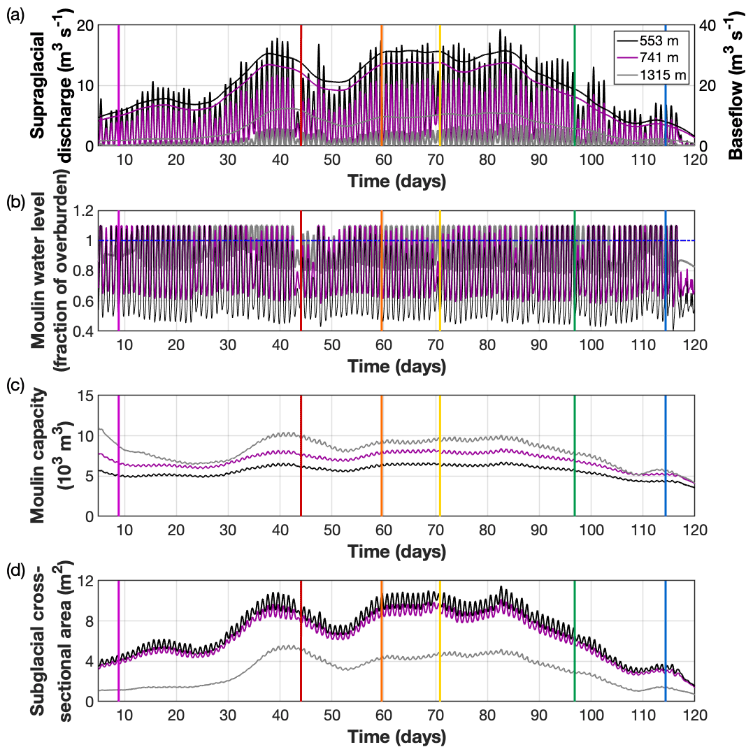
Figure 6 MouSh model runs with realistic supraglacial and ice conditions. The model runs are for a low-elevation Basin 1 (H_i=553 m; black lines), mid-elevation Basin 2 (H_i=741 m; purple lines), and high-elevation Basin 3 (H_i=1315 m; grey lines). (a) Supraglacial discharge into the moulin Q_in and prescribed base flow Q_base. (b) Moulin water level as a fraction of overburden. Note that the highest-elevation moulin exceeds the ice surface most days. (c) Moulin capacity, or the total moulin volume. (d) Subglacial channel cross-sectional area. Colored vertical lines indicate times in Fig. 7. Note x axes start on day 5.

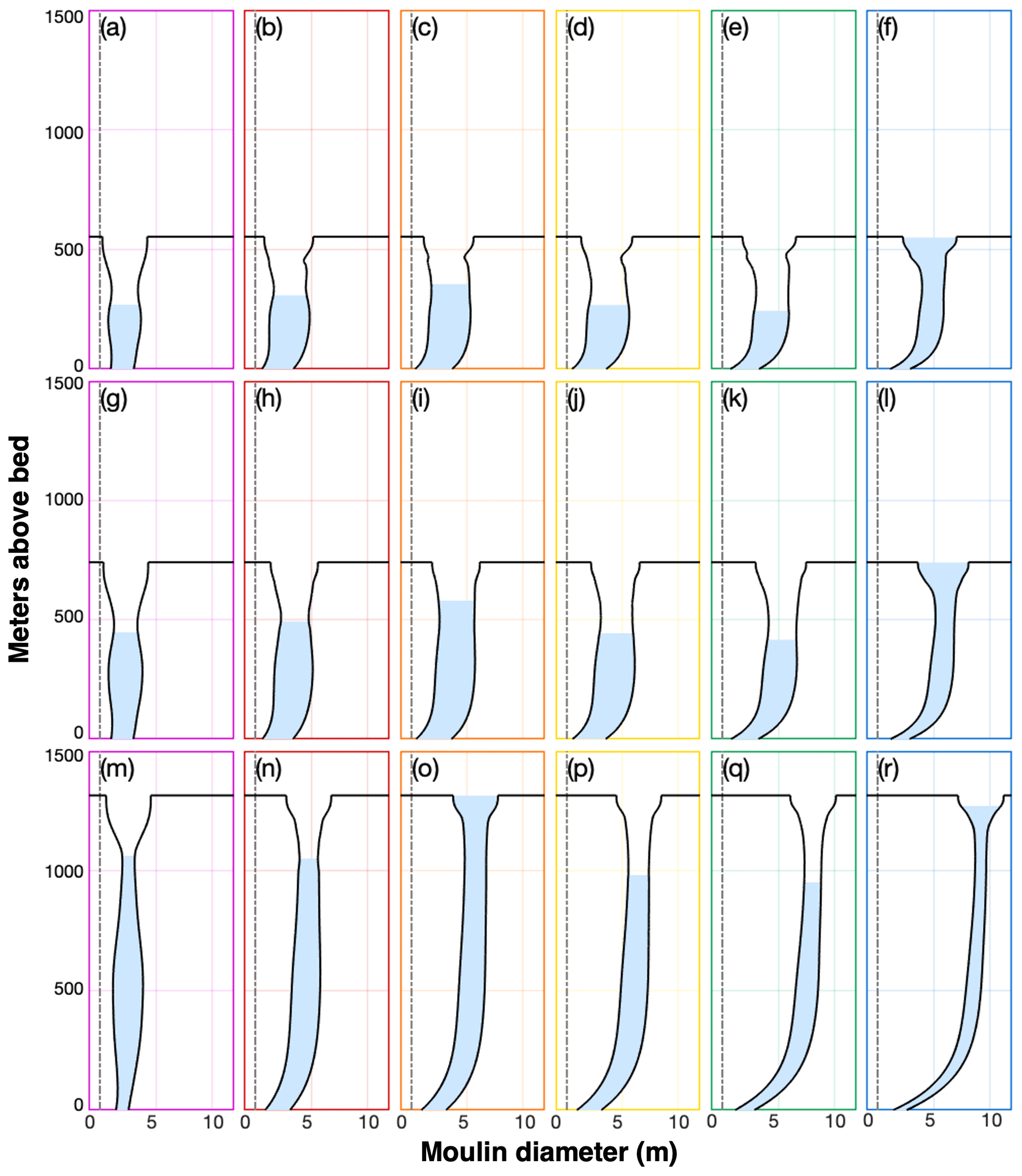
Figure 7 Evolution of moulin geometry over the melt season. Colored boxes correspond to the times indicated with colored vertical lines in Fig. 6. (a–f) Basin 1 with ice thickness of 553 m. (g–l) Basin 2 with ice thickness of 741 m. (m–r) Basin 3 with ice thickness of 1315 m. Axes are not to scale.

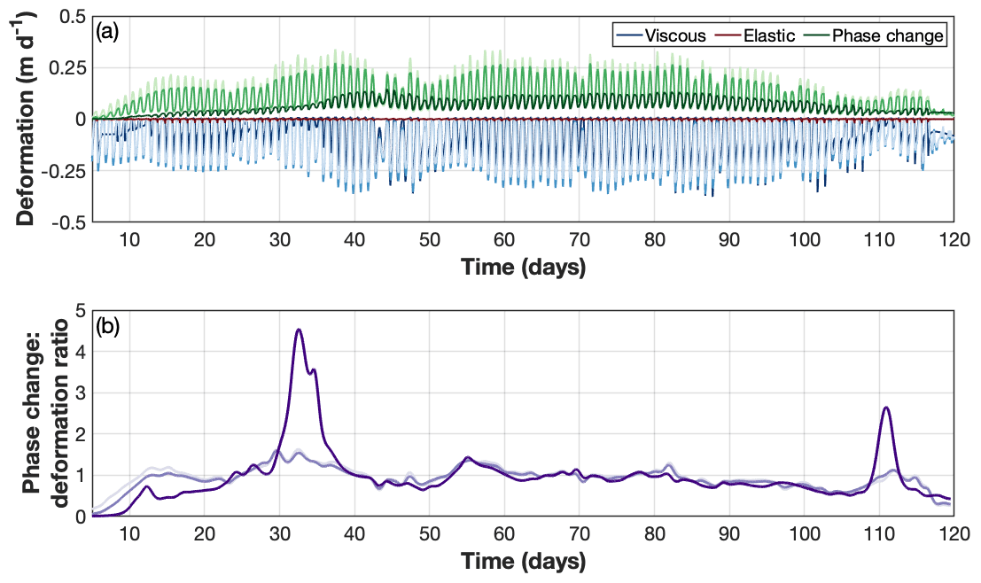
Figure 8 Time series of viscous, elastic, and phase change components of moulin evolution and their relative importance in determining moulin geometry. (a) Time-varying viscous (blues), elastic (reds), and phase change (melting, greens) components of moulin geometry. (b) The daily ratio of the total amount of phase change (melting above and below the water line) to total deformation (elastic plus viscous; shades of purple). Values above 1 indicate that melting dominates; values below 1 indicate that deformation dominates. Data are smoothed over 24 h. For both panels, light colors are for Basin 1 (H_i=553 m), medium colors for Basin 2 (H_i=741 m), and dark colors for Basin 3 (H_i=1315 m). Note x axes start on day 5.

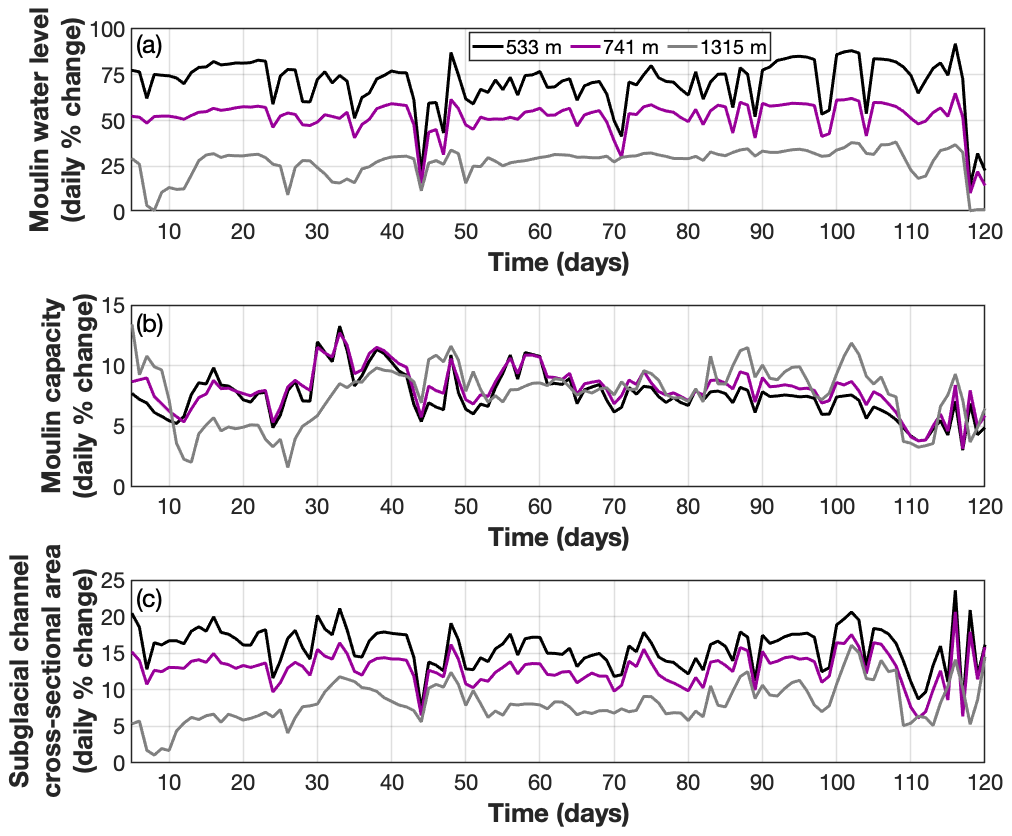
Figure 9 Daily percentage change in moulin variables relative to the daily mean value. (a) Daily percentage change in moulin water level relative to the daily mean water level for Basins 1, 2, and 3 (black, purple, and grey lines, respectively). (b) Daily percentage change in moulin capacity relative to the daily mean moulin capacity. (c) Daily percentage change in the subglacial channel cross-sectional area relative to the daily mean value. For (b) and (c), colors are as in (a).

2.5.4 Comparison to a cylindrical moulin

Subglacial models generally use a time-invariant vertical cylinder to represent moulins. To investigate and quantify the efficacy of our time-evolving moulin shape model, we drove MouSh and a static cylinder with the same meltwater inputs. We use the time-mean radius at the water level as the radius of the static cylinder; this is 1.6 and 1.4 m for Basin 1 and Basin 2, respectively. We compared the resulting moulin water level, moulin capacity, subglacial cross-sectional area, and meltwater input difference (due to melt generated within the model itself) across these runs. We compared the moulin water level values directly (cylindrical water level − variable water level) and moulin capacity by percentage difference (cylindrical − variable) $/$ (variable); differences are presented in Fig. 10.

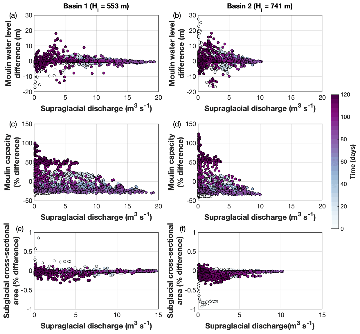
Figure 10 Difference between variable and fixed moulin geometries for Basins 1 and 2 (ice thicknesses of 553 and 741 m, respectively). The fixed moulins are cylinders with a fixed radius of 1.6 and 1.4 m for Basins 1 and 2, respectively, which are the time-mean radii at the mean water level for the variable moulins. In all instances, the difference is calculated as (cylindrical − variable) with instances of percentage difference calculated as (cylindrical − variable) $/$ (variable). (a, b) Difference in moulin water level for Basin 1 and Basin 2, respectively, plotted every hour. Negative values indicate periods where the variable moulin water levels are higher than those of the fixed cylindrical moulin. (c, d) Percentage difference in moulin capacity plotted every 2 h for clarity. When values are negative, the variable moulin is larger than the fixed cylindrical moulin.

2.5.5 Sensitivity to model choices

As part of MouSh development, we made several decisions about how to represent moulin geometry, water inputs, and the associated subglacial system that can directly impact the shape and water level of a modeled moulin. We test the impact of these decisions in a series of experiments, including (1) representing moulin cross-sectional area as a semi-elliptical, semi-circular “egg” instead of as a circle (Sect. 2.1); (2) the inclusion of elastic deformation (Sect. 2.2.1); (3) the use of a parabolic ice sheet profile to determine the surface slope and distance to terminus for a given ice thickness (Cuffey and Paterson, 2010); (4) the use of prescribed baseflow into the subglacial component of the model (Sect. 2.4); and (5) the use of a time-evolving subglacial channel (Sect. 2.4.2).

To explore the impact of our model choices for experiments 1–4, we perform a series of comparisons against a slightly modified seasonal run for Basin 1. This allows us to capture the effect of our choices during periods of increasing and decreasing Q_in. We change only the parameter of interest to isolate the effect on moulin water level and moulin capacity, the two variables that most directly affect water flow within the subglacial system. Further description of these runs is included in Supplement Sect. S2.2, and resulting differences are highlighted in Fig. S5.

The first two choices pertain to the complexity of the model, with our choices being more complex; simplification may be beneficial in some circumstances. In experiment 1, the model is initialized with the same circular geometry as the control run (Supplement Sect. S2.2.1), but melting above the water line is uniformly distributed around the moulin perimeter. Thus there is only one radius to evolve (Supplement Sect. S2.2.2). In experiment 2, we test model sensitivity to the inclusion of elastic deformation (Supplement Sect. S2.2.3).

Experiments 3–5 reflect the simplicity of the current subglacial hydrologic model and would be eliminated if MouSh were configured to function with either specific observational data or with a more comprehensive subglacial model. In experiment 4, we test using a subglacial channel length of one-half, and one and one-half the length defined in the control run (Supplement Sect. S2.2.4). In experiment 4, we prescribe a lower baseflow (Supplement Sect. S2.2.5).

In experiment 5, we examine the effect of an evolving versus a fixed-geometry subglacial channel (Supplement Sect. S2.2.6). The fixed subglacial channel cross-sectional area is set to 1.95 m². For these runs we use a simpler Q_in, the co-sinusoidally varying function described in Sect. 2.4.1. Details about this simplification are described in Supplement Sect. S2.2.6 with results in Fig. S6.

3 Results

3.1 Quasi-equilibrium and dependence on Q_in

Under a constant supraglacial input, the moulin water level, radius, and water capacity reach equilibrium within 15 d (red line, Fig. S2c). However, supraglacial inputs are rarely, if ever, uniform, so under constantly varying conditions, the moulin will reach a “quasi-equilibrium” state. This is a mean state (geometry, water level, deformation rates) with superimposed variability on the timescale of variations in Q_in alone. Therefore, if the forcing is diurnal, the moulin will exhibit diurnal variability from a mean state. The quasi-equilibrium state is also dependent on model characteristics and parameters (Sect. 3.2).

The magnitude and amplitude of Q_in alter the moulin water level and major radius at the mean water level (a proxy for moulin geometry) in predictable ways (Figs. S2 and S3). Increasing the diurnal amplitude of Q_in increases the diurnal variability and mean moulin water level (Figs. S2b, S4). This occurs due to the disparate timescales of ice deformation versus melting. The daily increase in Q_in raises the water level quickly because the moulin and subglacial channel are slow to expand by melting. Conversely, the nightly fall in Q_in is muted by a fast viscous contraction of the moulin and subglacial channel. This behavior drives the daily peak in moulin water level higher above the mean water level than the daily minimum water level falls below it (Fig. S2b). The “extra” time spent with higher water levels reduces the visco-elastic closure of the moulin while also increasing turbulent melting, resulting in a larger moulin, as indicated by the moulin radius at the mean water level (Fig. S2c). Higher diurnal amplitudes in Q_in magnify this effect.

As the Q_in magnitude increases, both the mean water level and its diurnal variability decrease (Fig. S3a and b). This occurs because the moulin becomes larger in response to increasing Q_in and subsequent increases in subglacial discharge. As the moulin and subglacial channel widen, they can readily accommodate the fluctuations in Q_in with lower variations in moulin water level. This accommodation is evident in the moulin radius at the mean water level (Fig. S3c). Higher Q_in magnitude drives a linear increase in melt rates within the moulin alongside nonlinear increases in visco-elastic deformation, causing an overall nonlinear increase in mean moulin water level (Fig. S4). However, when moulin water levels exceed flotation, the moulin grows due to both visco-elastic deformation and melting, resulting in a moulin larger than would be expected based on the equilibrium water level (blue line, Fig. S3c).

3.2 Sensitivity of MouSh to parameter values and deformational processes

A range of ice characteristics affect the time evolution of moulin geometry. These include the initial moulin size, temperature and viscosity of the ice column, viscosity of basal ice, friction factors, and ice thickness. Some of these factors are highly spatially variable (e.g., ice thickness) and others are poorly known (e.g., basal ice viscosity). We quantify the effect of these factors on moulin water level and moulin volume, moulin geometry, and subglacial channel cross-sectional area over both multi-day and diurnal timescales by performing multiple independent sensitivity studies.

We find that moulins reach a quasi-equilibrium, where the mean moulin water level and the moulin radius at this location oscillate consistently around a daily mean value, within 15–20 d of model initialization. The quasi-equilibrium value is independent of the initial moulin radius (Figs. 3a and b, 4a and b).

Two primary parameters affect the degree of viscous deformation in the moulin: the ice flow enhancement factor F^∗ and the ice temperature profile T_i(z). We tested a span of reasonable values representative of glacier and ice sheet ice (Table 1) and found a limited effect on moulin geometry. Equilibrium moulin water level, subglacial channel area, and their diurnal variabilities remain constant (<0.1 % change) over the tested range of these parameters (Figs. 3d, f, h and 4d, f, h). Moulin capacity and water storage show high sensitivity (∼100 %–150 % in equilibrium value and ∼100 %–200 % in diurnal range) across the range of F^∗ and T_i scenarios tested; a decrease in moulin capacity and water storage pair with an increase in the diurnal variability for these variables. For instance, varying F^∗ across an order of magnitude grew the equilibrium major radius by 26 % and shrank the equilibrium minor radius by 72 %, with a net effect that moulins had 65 % less volume and 58 % less water storage capacity in softer ice ($F^{\ast }=\mathrm{9}$) compared to harder ice ($F^{\ast }=\mathrm{1}$) (Fig. 3c and d). Similarly, the different ice temperature profiles we tested caused variations of 29 % in moulin major radius, 65 % in moulin minor radius, 63 % in moulin capacity, and 73 % in moulin water storage, with warmer ice hosting smaller moulins (Fig. 3e and f). We also varied Young's modulus E across 1 order of magnitude, but this affected moulin radius, water volume, and moulin capacity by ∼0.01 %. This is due to the low magnitude of elastic deformation overall compared to viscous deformation (Fig. 5g).

We find that moulin geometry is strongly sensitive to the choice of basal ice softness and the friction factors used within the moulin (f_m and f_oc). Melting due to the dissipation of turbulent energy is partially controlled by the friction factors chosen for the moulin walls. The friction factor above the water line (f_oc, “open channel”) does not significantly affect moulin water level (<0.1 % change for f_oc variations over 2 orders of magnitude), moulin volume (6 %), moulin water storage (0.1 %), or subglacial channel area (<0.1 %) over either long or diurnal timescales (Figs. 3m and n and 4m and n). However, like the deformational parameters, the open-channel friction factor does affect moulin radii, with the major radius growing by 50 % as the open-channel friction factor increases over 2 orders of magnitude, and the minor radius decreases by 24 %. This dampens the diurnal variability in the major and minor radii by 70 % and 24 %, respectively (Fig. 4m).

Increasing the friction factor below the water line (f_m) had similar effects to changing f_oc. Increasing f_m by 2 orders of magnitude increased the cross-sectional area of the moulin by 106 %, via a 10 % increase in the major radius and a 93 % increase in the minor radius. The water volume increased by 127 % and the storage capacity increased by 74 % (Fig. 3k and l) while the equilibrium water level and the subglacial channel area changed by <0.1 %. Increasing f_m also increased the diurnal variability of the moulin capacity and water storage by 130 % and 126 %, respectively, by increasing the diurnal differential melt rate (Fig. 4k and l).

The two parameters which have the largest impact on moulin water level are the basal ice softness A_sub and the moulin location on the ice sheet, described jointly by the ice thickness (H_i) and distance from the terminus (L). This sensitivity indicates an interplay among these parameters, the subglacial hydraulic gradient, and moulin water level.

We varied basal ice softness A_sub by 2 orders of magnitude. Softer basal ice increased the size and storage capacity of the moulin: the major radius by 23 %, the minor radius by 23 %, the total capacity by 41 %, and the stored water volume by 88 % (Fig. 3i and j). These changes also increased the equilibrium water level by 34 % and the subglacial channel area by 14 %, unlike tests on englacial parameters (F^∗, T_i, and E), which did not affect the water level or subglacial channel area. These changes occur because softer basal ice increases the rate of subglacial creep closure, which reduces subglacial channel cross-sectional area, which reduces water throughflow in the moulin and increases water level, which in turn reduces the amount of viscous and elastic radial closure in the moulin. Increasing the basal ice softness to approximately 10⁻²³ Pa⁻³ s⁻¹ increases the diurnal variability in the sizes of the subglacial channel and moulin (Fig. 4i and j); however, increasing A_sub above this value causes moulin water levels to rise high enough that diurnal fluctuations are truncated by the ice thickness, resulting in an observed decrease in diurnal range that would not be present in thicker ice (Fig. 4j).

We co-varied ice thickness and distance from terminus using a parabolic approximation for a perfectly plastic ice surface profile (Cuffey and Paterson, 2010); this covariance alters the hydraulic gradient of the system. Changes in ice thickness from 670 to 1570 m (80 %) increase the equilibrium subglacial channel area by 24 % and increase equilibrium water levels by 203 % (Fig. 3o and p). Increasing ice thickness and distance from the terminus increases the moulin major and minor radii by 7 %, increases moulin volume by 93 %, and increases moulin water storage by 235 % (Fig. 4p). We also find significant increases in diurnal variability in subglacial channel size (29 %), water level (178 %), moulin radii (major radius 84 % and minor radius 24 %), moulin volume (130 %), and moulin water storage (750 %) in thicker ice farther from the terminus (Fig. 4o and p).

Overall, we find that MouSh-modeled moulins are primarily sensitive to the friction factors for water flow through the moulin, basal ice softness, and location on the ice sheet (ice thickness and distance from the terminus). The results are less sensitive to englacial material factors that govern elastic and viscous deformation. The observed sensitivity to the ice thickness and distance from terminus signals that moulin geometry can vary spatially. The sensitivity to friction factors and basal ice softness indicates that the values of these poorly constrained parameters should be carefully chosen and kept in mind when interpreting model output.

3.2.1 Contributions to moulin shape

Figure 5 illustrates the role of each process, phase change, viscous deformation, and elastic deformation, in determining moulin radius under different hydraulic potential gradients with median model values (Table 1). Elastic deformation has little impact on moulin shape or variability (Fig. 5f and g) and is persistently an order of magnitude smaller than either viscous deformation or radius evolution due to phase change. Viscous deformation and phase change due to melting peak near the daily maximum water line, with the daily mean of each increasing with increasing ice thickness (Fig. 5f); however, the opposite effect is observed near the bed, where lower mean water levels in moulins in thinner ice increase viscous deformation at the bed; melting also increases in response to the higher hydraulic potential gradient.

At any given depth, viscous deformation and phase change due to melting are similar below the waterline; however, the diurnal variation in these parameters is quite different (Fig. 5g). At the mean water level, moulin growth due to melting varies less than 0.04 m d⁻¹, with the shape of the diurnal variability dependent on the parameterization of melting both above and below the water line. In contrast, viscous deformation displays diurnal variations between 0.08 m d⁻¹ in the thinnest ice and more than 0.21 m d⁻¹ in the thickest ice.

3.3 Moulin shape in different environments

We modeled the seasonal growth and collapse of moulins in a range of environments across the GrIS using realistic melt forcings derived for the 2019 melt season (Sect. 2.5.3). These model runs varied with respect to ice thickness, moulin distance from the terminus, baseflow, and magnitude, diurnal range, and seasonal evolution of supraglacial inputs (Table 2; Fig. 6a). Overall, we find that moulin setting affects the scale of diurnal and seasonal variability in the size and water capacity of moulins as well as the evolution of subglacial channels (Figs. 6 and 7).

The sizes of all three modeled moulins reach equilibrium with the melt forcing within ∼15 d of the onset of the melt season (Fig. 6b and c). As the water flux increases over the next few weeks, each moulin grows in response to increasing supraglacial inputs, both diurnally and with a long-term trend, although this growth is more significant in thicker ice (Figs. 6c and 7). The subglacial channel grows with a similar pattern, but interestingly, the setting and fluxes of Basin 1 and Basin 2 result in very similar subglacial channel cross-sectional areas despite different moulin water levels and capacities (Fig. 6d).

Although the three moulins all evolve in a similar fashion, there are differences in moulin capacity, water level (Fig. 6), overall moulin geometry (Fig. 7), and the magnitude of englacial deformation (Fig. 8). Basin 3 exhibits the largest seasonal change in moulin capacity in part because a lower supraglacial input and subglacial hydraulic gradient result in a smaller subglacial channel and periods where moulin water level is above flotation (Fig. 6). This causes substantial variability of viscous deformation while limiting variations in melt due to changing moulin water level (Fig. 8a). One of the largest periods of Basin 3 moulin growth occurs starting at day 30. During this period, supraglacial inputs experience a step change (Fig. 7a); moulin water levels stayed near flotation and were less variable for several days (Fig. 7b), keeping effective pressure near zero and retarding deformation (Fig. 8a). In this case, viscous deformation hovers around zero and causes moulin opening, resulting in a high ratio of elastic to viscous deformation and a high ratio of phase change to viscous deformation (purple line in Fig. 8b). Similar behavior also occurs around day 110. Basins 1 and 2 exhibit smaller seasonal variations in moulin capacity because the ratio of melting to deformation stays near 1 until near the end of the season (Fig. 8b). This occurs because viscous deformation in Basins 1 and 2 is only slightly lower than in Basin 3, and melt rates tend to be higher (Fig. 8a) due to increased subglacial discharge associated with a higher hydraulic gradient. Further, there are fewer periods where water levels above flotation drive viscous opening.

Each moulin has a different daily mean capacity (Fig. 7c). This, in addition to differences in supraglacial inputs, ensures that daily moulin water level variations are substantially different across moulins. Basin 1 exhibits the largest variation in daily moulin water level, followed by Basin 2 (Fig. 9a). Basin 3 shows the lowest daily change; however, this is due at least in part to the fact that water overtops the moulin nearly daily (Figs. 6b and 7m and n). Changing water levels drive changes in moulin and subglacial capacity. Over the melt season, daily change in moulin capacity can be as low as 2 % during lulls in diurnal melt variability (Basin 3) or as high as 12 % following a recovery from a low melt day (Basin 1; Fig. 9b). However, in general all moulins display a similar daily change in capacity of ∼5 %–10 %.

The subglacial system undergoes diurnal variations in channel size between 1 % and 20 % (Fig. 9c). These changes are similar in magnitude to daily capacity changes within the moulin but exhibit more variability across ice thicknesses. Like changes in moulin capacity, these variations are related to the daily changes in moulin water level (Fig. 9a). This suggests that the time evolution of moulin geometry dampens the diurnal pressure fluctuations that drive subglacial channel growth and collapse. Evidence for this can be seen in the temporal pattern of moulin water level and subglacial channel cross-sectional area (Fig. 9a and c).

3.4 Comparison to cylindrical moulins

To examine the role moulin evolution plays in modifying the subglacial hydrologic system, we compared moulin water levels, moulin capacity, and subglacial channel size between model runs with a fully evolving moulin and runs with a static cylindrical moulin. We performed these tests with realistic melt inputs based on the 2019 melt season (Sect. 2.5.3), at moulins with low and moderate ice thicknesses (553 m – Basin 1 and 741 m – Basin 2). We defined the radius of the static cylinder as the mean radius at the mean water level: 1.6 and 1.4 m for Basins 1 and 2, respectively. This results in fixed moulin cross-sectional areas (∼6 to 8 m²) within the range of spatially invariant moulin cross-sectional areas ∼2–10 m² often prescribed in subglacial models (e.g., Andrews et al., 2014; Banwell et al., 2013; Bartholomew et al., 2012; Cowton et al., 2016; Meierbachtol et al., 2013; Werder et al., 2013).

Comparison of moulin water level and capacity between static cylindrical and evolving moulins shows differences on both the diurnal and seasonal timescales (Fig. 10). The differences in moulin water level (both positive and negative) are generally greatest during lower supraglacial inputs at the beginning and end of the melt season, with the relatively limited differences occurring during the highest discharges (Fig. 10a and b). These values are both positive, indicating that the static radius moulin has higher water levels, and negative, indicating that the evolving moulin has higher water levels. Differences in moulin water level can reach nearly 20 m but are most commonly below 10 m. The seasonal mean water level difference between the static cylindrical and evolving moulin in both basins is less than 1 m.

Moulin capacity also displays a clear seasonal pattern; in both basins, the static cylindrical moulin is larger than the evolving moulin at the beginning of the melt season, with the evolving moulin gradually growing larger as the melt season progresses (Fig. 10c and d). After peak melt (day ∼60), the evolving moulin begins to viscously close and gradually becomes smaller than the static cylindrical moulin. The static cylindrical moulin can be more that 100 % larger than the variable moulin during the tails of the melt season, with the evolving moulin becoming 36 % (Basin 1) and 42 % (Basin 2) larger than the static cylindrical moulin during mid-melt season. Overall, the mean capacity difference between the static cylindrical and evolving moulin is less than 5 %, with the static cylindrical moulin being slightly larger.

The radii of the cylindrical moulins were chosen to minimize differences with the evolving moulins. This is evident by the limited long-term differences between the two moulins in both Basin 1 and Basin 2. As such, there are limited differences (<1 %) between the modeled subglacial channels. We expect the difference in moulin water level, moulin capacity, and subglacial geometry to change if the static cylindrical moulin geometry is poorly chosen, if the different or different experimental parameters are used, or if the setting changes (e.g., different hydraulic gradients). For example, we use commonly used values of ice softness for both the moulin and subglacial channel; however, these values are poorly known, and their choice can directly impact the relative importance of moulin shape in dictating moulin water levels and subglacial channel size (Fig. 4).

3.5 Impact of model choices on moulin geometry

Chosen parameterizations have the potential to impact the representation of moulin water level and capacity (Supplement Sect. S2). Overall, we find that a circular geometry has limited impact on moulin water level, with the circular moulin exhibiting water levels that are less than 3 m higher than the egg-shaped moulin, although in nearly all instances the difference is less than 0.5 m (Fig. S5a); however, the impact on capacity is slightly larger (the circular moulin is up to 31 % smaller) and displays a seasonal trend as the egg-shaped moulin elongates along its elliptical axis (Fig. S5b).

Elastic deformation within the moulin is small (Supplement Sects. S1 and S2.2.3; Fig. 8a). Excluding elastic deformation has a negligible impact on moulin water levels and moulin capacity (<1 %; Fig. S5c and d).

In contrast to the previous choices, the distance from the terminus L and the prescribed baseflow Q_base can have a substantial impact on moulin water level and capacity (Fig. S5e–h). Distance from the terminus is defined by the position of a given moulin on the ice sheet and as such is not a choice or parameter per se; however, it does directly influence the hydraulic gradient. A shorter L increases the hydraulic gradient and reduces both moulin water levels and capacities (Fig. S5e and f). Baseflow is used here to mitigate the use of a simplistic subglacial hydrology model. Reducing the baseflow within the subglacial system increases moulin water levels and reduces moulin capacity (Fig. S5g and h).

Finally, we examine the impact of fixing the subglacial channel cross-sectional area S. Experimental results using a fixed S and a seasonally evolving melt curve resulted in unrealistically low or zero water levels during low, early season Q_in and complete viscous collapse of the moulin if the subglacial channel size was prescribed to be too large, or persistently high (always above the ice thickness) water levels and runaway moulin growth if the subglacial channel was prescribed to be too small. Therefore, we explore the impact of fixing S using a constant mean Q_in with an overlaid diurnal variability (Supplement Sect. S2.2.6). With constant variability, we can easily prescribe the fixed S to be the mean value of the time-varying subglacial channel S (1.95 m). In this instance, the fixed S experiment displays a similar mean moulin water level but lower diurnal variability than the experiment with a time-varying S (Fig. S6). Further details are included in the Supplement Sect. S2.

4 Discussion

4.1 Timescales of moulin formation and evolution

We consider the formation timescales of moulins in the context of the shape evolution of a mature moulin. Using MouSh, we find that in the absence of external forcing, such as time-variable Q_in, the size of a moulin reaches its equilibrium value in ∼15 d depending on ice and supraglacial input conditions and initial moulin geometry (Figs. 5g, S2 and S3). This relaxation time is comparable to the Maxwell time for ice (10–100 h), as expected for a linear visco-elastic system. Our relaxation time also compares well to the equilibration timescale defined by Covington et al. (2020) for their modeled moulin–subglacial conduit system, which Trunz (2021) found to be 1–20 d. The most realistically sized moulins in Trunz (2021) had relaxation times closer to 1 d. Their modeled system was governed solely by melt and viscous deformation; however, elastic deformation in MouSh is small, explaining why our relaxation times are comparable.

If the process of moulin formation occurs on a timescale shorter than the 15 d relaxation time, the formation process likely will not influence the overall form of the englacial system at equilibrium. This time range includes hydrofracture during rapid lake drainage (∼2 h) and slow lake drainage ($<\sim \mathrm{6}$ d, e.g., Selmes et al., 2011) and likely also the reactivation of existing moulins in ensuing melt seasons, which, based on the timing difference between surface melt onset and ice acceleration, occurs over multiple days (Andrews et al., 2018; Hoffman et al., 2011). On the other hand, moulin formation by cut-and-closure occurs over years to decades (Gulley et al., 2009), well above the MouSh relaxation time and the Maxwell time for ice, is more likely to create subvertical englacial channels. The interdependence of formation and evolution of these moulins gives us less confidence in applying our model to moulins with cut-and-closure origins. Those moulins primarily occur in temperate near-surface ice within polythermal glaciers (Gulley et al., 2009) and have not been reported on the GrIS.

4.2 Comparison of modeled and observed moulin geometries

Field observations suggest that moulin geometry evolves a high degree of complexity. Observations include anecdotes of difficulty deploying sensors to the bottom of a moulin, which suggests the presence of kinks, ledges, knickpoints, and other twists (Andrews et al., 2014; Covington et al., 2020; Cowton et al., 2013). Complex geometry revealed during mapping moulins above the water line further suggests that moulins are not simply vertical cylindrical shafts (Covington et al., 2020; Moreau, 2009).

The MouSh model suggests that the energy transfer from turbulent meltwater entering the moulin to the surrounding ice drives highly spatially variable melt rates above the water line. We incorporated the open-channel melt module to allow a large opening to emerge above the water line (Figs. 5a–e and 7). When we run MouSh without the open-channel module, the surface expression of the moulin becomes dependent on surface stresses and can in some instances pinch closed. The open-channel module also permits the development of an egg-shaped geometry, which is supported by seismic observations and a resonance model of a moulin, which suggests that moulins may increase in ellipticity over time (Röösli et al., 2016).

The value of the open-channel friction factor and the portion of the moulin perimeter over which melting occurs directly affect the size of the upper, air-filled chamber of the moulin. This is distinctly different from when the moulin is modeled as circular and open-channel melting is applied uniformly around the perimeter (Fig. S5b). MouSh can predict ledges at the top and bottom of a consistent diurnal range in water level. Thus, we infer that energetic subaerial water flow drives formation of moulin complexity above the water line, and diurnal fluctuations around a steady multi-day water level drive ledge formation through a differential in melting and viscous deformation above and below the water line. Energetic water flow is commonly observed at stream-fed moulins near the peak of the melt season (Pitcher and Smith, 2019) or during and immediately following rapid lake drainage (Chudley et al., 2019). This suggests that complex moulin geometries form during periods of relatively consistent water supply. Conversely, multi-day rises in water level, driven by either the surface water supply or the basal water supply (baseflow), can erase geometric complexities such as ledges, as seen in MouSh results during a melt event (Fig. 7).

Above the water line, explored moulins in Greenland show highly variable shapes from moulin to moulin (e.g., Covington et al., 2020). Some moulins, for example the FOXX moulin, are nearly cylindrical within the explored depth (∼ 100 m), with radii comparable to what we model (∼1.5 m). Others open some tens of meters below the surface to large caverns with radii approaching 10 m, a similar morphology to karst caves with narrow entrance shafts (Covington et al., 2020). MouSh can produce large openings above the water line if we use a suitably large open-channel friction parameter, although we lack a narrow entrance shaft and substantial vertical variability. These differences are due to the inability of model parameterizations to represent complex geometries such as scalloping, plunge pools, and knickpoint migration (Gulley et al., 2014; Mankoff et al., 2017). Indeed, instead of modeling processes above the water line as turbulent open flow, they could, in the future, be modeled using geomorphic parameterizations to model waterfall migration, perhaps resulting in the clearer development of steps and plunge pools. This would require development and inclusion of a supraglacial channel model as well.

Below the water line, MouSh results indicate that a cylinder is a reasonable representation for newly formed moulins in Greenland. However, there are two caveats. First, moulin cross-sectional area, and thus water storage capacity, can vary substantially over the course of a day or season (Figs. 6c and 9b), and features such as englacial crevasses and reservoirs may be present (e.g., McQuillan and Karlstrom, 2021). Second, in instances where moulins are reactivated over multiple melt seasons (Chu, 2014; Smith et al., 2017), there may be substantial deformation, as suggested by cable breakage in boreholes (Ryser et al., 2014; Wright et al., 2016).

Observations show a wide range of moulin volumes above the water line, and moulin volumes predicted by MouSh are sensitive to the consideration of turbulent melting and associated parameter choices. Given the flexibility of model results, we should continue to rely on field exploration to measure moulin size and geometry above the water line and make efforts to constrain the parameters that affect sub-seasonal growth and collapse. MouSh results below the water line are less sensitive to uncertain parameter values, so direct observations of underwater geometry would be less relevant for model validation than subaerial observations. Overall, results from the MouSh model demonstrate that moulin geometry evolves substantially over diurnal to seasonal timescales and varies with ice conditions.

4.3 Diurnal water level oscillations and moulin size

Moulin geometry can directly alter the relationship between meltwater inputs and moulin water level changes – the primary driver of subglacial channel evolution (Andrews et al., 2014; Cowton et al., 2013). Field measurements of moulin water levels indicate diurnal oscillations of 3 %–12 % (Covington et al., 2020), ∼25 % (Andrews et al., 2014), and >20 % (Cowton et al., 2013) of overburden pressure, with mean water levels of ∼70 % of overburden. These diurnal fluctuations are larger than those observed in boreholes, which are generally, though not always, thought to sample inefficient components of the subglacial hydrologic system (Andrews et al., 2014; Meierbachtol et al., 2013; Wright et al., 2016).

Our model results agree well with observations of moulin water level: diurnal fluctuations of approximately 25 % to 50 % of overburden pressure, with larger absolute oscillations occurring in thicker ice. To explain larger-than-expected daily oscillations (∼10 %) in thinner ice, Covington et al. (2020) incorporated moulin cross-sectional area as a free parameter into their model. Matching field measurements of water level required a modeled moulin radius of ∼5 m (∼75 m² cross-sectional area) at ice thickness of 500 m and a much larger moulin (radius ∼20 m and cross-sectional area ∼1500 m²) at ice thickness of 700 m (Covington et al., 2020). For comparison, MouSh predicts average radii ∼1.4 m (∼6 m² cross-sectional area) in similar ice thicknesses using parameters described in Table 2, including substantially larger meltwater inputs compared to Covington et al. (2020). The drastic differences in moulin size despite similar variations in diurnal water level between our study and Covington et al. (2020) cannot easily be attributed to a single factor but may be explained by our limited ability to model processes above the water line, our inclusion of baseflow (Fig. S5f and g), substantial differences in meltwater input (e.g., Figs. S2 and S3), fluctuations in moulin capacity (Covington et al., 2020, use a fixed moulin geometry), or that their measured water levels were not from the same moulin they mapped englacially. However, our results suggest that an evolving moulin capacity may be important to represent realistic moulin water levels and capacity (Fig. 10). Thus, to match observed moulin water level fluctuations without evolving the moulin geometry, a fixed cross-sectional area substantially larger than the associated subglacial channel may be necessary, as reported in Covington et al. (2020).

4.4 Magnitude of viscous moulin deformation

Viscous and elastic deformation drive moulin closure. The role of elastic deformation in the glacial hydrologic system is discussed below; viscous deformation is the primary closure mechanism of moulins, boreholes, and subglacial channels (e.g., Catania and Neuman, 2010; Paterson, 1977; Shreve, 1972), with viscous deformation dependent on local effective pressure, ice characteristics, and the geometry of the feature of interest (Flowers, 2015). Viscous deformation within our moulin varies in response to meltwater inputs (Figs. 5g and 8a) with the highest deformation rates occurring at the water line (Fig. 5f) because at the water line, inward cryostatic pressure is least offset by outward hydrostatic pressure (see Eq. 3).

During our realistic runs, viscous deformation can exceed 0.25 m d⁻¹ for short periods of the day at all three moulin locations (Fig. 8a). These deformation rates are substantially larger than measured borehole deformation rates for the primary reasons that boreholes are often at or above flotation due to high subglacial water pressures (e.g., Ryser et al., 2014) or because creep measurements are recorded in much smaller boreholes in colder ice (e.g., Paterson, 1977).

A previous moulin modeling effort focused on understanding moulin closure rates (Catania and Neumann, 2010). Their results indicate that an air-filled moulin will close within a single day at the bed. However, in this instance there is no opposing hydrostatic pressure. While our modeled closure rates are similar to those calculated by Catania and Neuman (2010) near the surface, the moulins modeled here always contain water even at the end of the melt season (Fig. 6b). This continued retention of meltwater is in line with borehole observations that subglacial pressures tend to be highest outside the melt season (Downs et al., 2018) and preclude the presence of completely air-filled moulins in areas where viscous deformation rapidly shuts down the hydrologic system as supraglacial inputs fall.

4.5 The role of elastic deformation in ice sheet hydrology

Our model results indicate that the equilibrium moulin geometry is dictated by a balance of visco-elastic deformation and turbulence-driven melting (Figs. 5 and 8). In both the sensitivity study and realistic model experiments, visco-elastic deformation generally closes the moulin, while melting of the surrounding ice consistently opens the moulin. The exception is when moulin water levels exceed flotation, in which case all three mechanisms open the moulin. In all model runs, we find that the rates of viscous deformation exceed elastic deformation by 3 to 4 orders of magnitude (Figs. 5g and 8). Elastic deformation rates are greatest near the water line and at the bottom of the ice column, where stress conditions are similar to those in subglacial models, at a few centimeters per year of closure within a moulin of radius ∼1 m. This moulin size is comparable to that of a typical subglacial channel in our model (A∼2 m², or radius 1.1 m), implying that elastic closure of a subglacial channel would also amount to a few centimeters per year. Elastic closure rates scale linearly with moulin radius; thus, larger moulins or channels would undergo commensurately faster elastic closure. The contribution of elastic deformation relative to viscous deformation increases with increasing ice thickness (Fig. 5f); at H_i=670 m, viscous deformation is 4000 times larger than elastic deformation at the water line, while at H_i=1570 m, it is 2000 times larger.

Current subglacial hydrology models represent subglacial channel development (opening) by turbulent energy dissipation and destruction (closing) by viscous deformation alone. However, work involving elastically responding storage elements or elastic flexure of the ice sheet has occurred (Clarke, 1996; Dow et al., 2015), and there have been efforts to use elastic deformation or fluid compressibility to improve numeric stability of channel equations (Clarke, 2003; Spring and Hutter, 1981, 1982). Interestingly, Clarke (2003) chose to use fluid compressibility due to model integration times. Yet, elastic deformation has generally been omitted from current models of glacial hydrology, even when modeling rapid changes in meltwater inputs (<1 d; e.g., Hewitt, 2013; Hoffman et al., 2016; Werder et al., 2013). Our investigation of the role of elastic deformation in diurnally closing moulins, particularly in thicker ice (Figs. 8b and S5c and d), suggests that its exclusion from subglacial channel models should cause errors of <0.1 % and is warranted. On length scales considerably larger than ∼1 m moulins, as well as in problems where elastic flexure is more central to the geometry, elastic deformation remains important. These applications include ice shelves (e.g., Reeh et al., 2003; Walker et al., 2016), large marine-terminating glaciers (Christmann et al., 2021), crevasse opening (Poinar et al., 2017), and rapid supra- and subglacial lake drainage (Dow et al., 2016, 2015; Lai et al., 2021).

4.6 Moulin geometry and the englacial void ratio

Subglacial hydrology models use an englacial void ratio parameter to represent bulk storage and release of meltwater in the englacial system (see Flowers and Clarke, 2002, for the best description). Because the englacial void ratio acts as short-term, pressure-dependent storage for subglacial models, it can improve the representation of diurnal water pressure fluctuations in subglacial models (Flowers and Clarke, 2002). This parameter represents bulk behavior and is usually tuned by comparing to local observations (e.g., Bartholomaus et al., 2011; Hoffman et al., 2016; Werder et al., 2013). The inclusion of time-varying moulin geometry, potentially in addition to time-varying representation of englacial fractures (Gajek et al., 2021), which evolve in response to meltwater inputs and subglacial pressures, could reduce subglacial model dependence on this parameterized englacial storage, particularly in light of observations of time-varying englacial features (Church et al., 2020) and meltwater content (e.g., Vanková et al., 2018).

MouSh demonstrates that moulin capacity can vary both seasonally and during large variations in supraglacial input. Moulin growth rates are largest particularly when water levels are above flotation, when both melting and viscous deformation work to increase moulin capacity. Our results show that moulin capacity changes by up to 13 % daily under realistic conditions (Fig. 9b) and 87 % to 138 % over the melt season (Fig. 6c). These variations in moulin shape and size may explain difficulties with modeling subglacial behavior during melt events (Cowton et al., 2016), which are sometimes addressed by temporarily increasing englacial storage (Hoffman et al., 2016). Our results with MouSh suggest that modeling moulin shape alongside the evolution of the subglacial system could potentially improve the representation of subglacial pressures, especially during periods of large meltwater variability; however, additional development is necessary to explore the impact of multiple moulins evolving along with the subglacial system.

Practical limits on model complexity or computational costs may preclude fully time-evolving moulin geometries. While not ideal, an arbitrary static shape may be preferable to a static cylinder (Trunz, 2021). Therefore, we interpret our moulin shape results (Fig. 7) to recommend a representative shape for a static moulin. Below the water line, a cylinder is a reasonable approximation, especially in thinner ice or for newly made moulins, for which full-column ice deformation is minimized. Above the water line, moulin shape is widely variable in time, by location, and across parameter combinations. It is especially sensitive to the friction parameter for open-channel flow (Figs. 3m and 4m), with low friction values making bottle-shaped moulins that have narrow necks above the water line and larger chambers below the water line and high friction values making goblet-shaped moulins with open rooms and amphitheaters above the water line atop a narrower geometry below the water line. Exploration of Greenland moulins to date has uncovered multiple goblet-shaped moulins and a few instances of near-cylindrical moulins but no bottle-shaped moulins (Covington et al., 2020; Moreau, 2009; Trunz, 2021). Overall, our MouSh results support goblet-shaped moulins, although with great variation in the height and width of the upper chamber.

4.7 Limitations of the current MouSh englacial – subglacial model

Moulins are a dynamic component of the channelized englacial–subglacial system; therefore, explicitly modeling their evolution can improve the fidelity of glacial hydrology models. MouSh currently uses a single subglacial channel to represent the entire subglacial system, limiting its accuracy. An optional baseflow term, which parametrizes subglacial water flow from surrounding regions, improves MouSh performance. This baseflow, added directly to the subglacial channel, is necessary to produce realistic equilibrium water levels with the realistic supraglacial inputs we prescribed (Fig. 6a). The baseflow value we used does not explicitly represent any specific process because our model runs resolve only a single moulin connected to a single channel, whereas in the real world, multiple moulins feed a network of channels. The idealized baseflow term conceptually connects to multiple potential water sources, including (1) basal melting from geothermal and frictional heating, (2) supraglacial water delivered via nearby moulins that are connected to the same subglacial channel, and (3) water that moves from the channelized system to the surrounding inefficient system at high pressures and then flows back into the subglacial channel at lower water pressures (Hoffman et al., 2016; Mair et al., 2001, 2002; Tedstone et al., 2015).

The addition of baseflow maintains a larger, less variable subglacial channel. This can alternately be achieved by lessening the local hydraulic gradient, thus increasing the mean water pressure along a given reach. Such behavior may locally occur where one subglacial channel enters another in an arborescent network (Fountain and Walder, 1998). MouSh currently does not have an interconnected network of channels; however, this is under development (Trunz, 2021).

We use a highly simplified model of the subglacial hydrology system: a single channel that connects the moulin to the ice sheet margin. Yet, MouSh results clearly indicate that including and evolving a moulin can alter the hydraulic gradient of the subglacial system via time-varying storage in the moulin (Fig. 10), though in our current single-moulin configuration, there is limited impact on subglacial channel geometry. Further, MouSh currently lacks a distributed system, which limits its fidelity for assimilating daily meltwater volumes into the subglacial system; realistically, the channelized subglacial system cannot always accommodate the full volume of meltwater produced during summer days, and a portion of this water goes into the distributed system (e.g., Mair et al., 2001, 2002). In our model, however, when the system is overwhelmed, the water level in the moulin rises above what is typically observed, and sometimes even exceeds the height of the ice (Figs. 6b and S4b). The melt-driven opening and creep closure processes in the subglacial model explain this behavior: a lower water input to the moulin (Q_in) lowers the water flux into the subglacial system (Q_out), which lowers the melt rates that keep subglacial channels open, reducing the size of the subglacial channels and thus further reducing the subglacial water flux. This increases the water level in the moulin. Thus, a reduced rate of surface melt can counterintuitively raise the modeled water level (Fig. 6, ∼ day 30), whereas in reality, much of that water would enter the inefficient subglacial hydrologic system when moulin water levels exceed flotation. If the moulin model were coupled to a two-component subglacial model that represents the inefficient system alongside the channelized system, we would anticipate a much-improved ability to assimilate a wide range of meltwater input rates.

5 Conclusions

Results from the MouSh model show that moulins are not static cylinders. Daily fluctuations in moulin capacity change the water volume held in the englacial hydrologic system, which in turn influences the evolution of the subglacial channels that moulins feed. When we represent a moulin as a static cylinder in our englacial–subglacial hydrology model, these daily fluctuations can be overestimated or underestimated, affecting the volume of water stored englacially and the hydraulic gradient of the subglacial system. Modeled moulin size and shape may provide a more realistic representation of moulin water level and the englacial void ratio commonly used in subglacial hydrology models, particularly with future efforts to improve the parameterization of moulin development above the water line. This could be achieved by using an englacial hydrology–channelized subglacial system model, such as the MouSh model we present here, to characterize variability in moulin size and shape, or by coupling moulin models to more complete models of the subglacial system (channelized, distributed, and optionally weakly connected) to make a unified englacial–subglacial hydrology model system. Improving the representation of the englacial–subglacial system to explicitly include moulins would have the greatest efficacy during periods of rapidly varying supraglacial input (e.g., during the beginning and end of the melt season and during melt events) and in inland areas with thick ice and high overburden pressures. These situations are coincident with where subglacial models without moulins, or with implicitly static moulins, tend to perform poorly.