Proper orthogonal decomposition of ice velocity identifies drivers of flow variability at Sermeq Kujalleq (Jakobshavn Isbræ)

The increasing volume and spatio-temporal resolution of satellite-derived ice velocity data have created new exploratory opportunities for the quantitative analysis of glacier dynamics. One potential technique, proper orthogonal decomposition (POD), also known as empirical orthogonal functions, has proven to be a powerful and flexible technique for revealing coherent structures in a wide variety of environmental flows. In this study we investigate the applicability of POD to an openly available TanDEM-X/TerraSAR-X-derived ice velocity dataset from Sermeq Kujalleq (Jakobshavn Isbræ), Greenland. We find three dominant modes with annual periodicity that we argue are explained by glaciological processes. The primary dominant mode is interpreted as relating to the stress reconfiguration at the glacier terminus, known to be an important control on the glacier's dynamics. The second and third largest modes together relate to the development of the spatially heterogenous glacier hydrological system and are primarily driven by the pressurisation and efficiency of the subglacial hydrological system. During the melt season, variations in the velocity shown in these two subsidiary modes are explained by the drainage of nearby supraglacial melt ponds, as identified with a Google Earth Engine Moderate Resolution Imaging Spectroradiometer (MODIS) dynamic thresholding technique. By isolating statistical structures within velocity datasets and through their comparison to glaciological theory and complementary datasets, POD indicates which glaciological processes are responsible for the changing bulk velocity signal, as observed from space. With the proliferation of optical- and radar-derived velocity products (e.g. MEaSUREs, ESA CCI, PROMICE), we suggest POD, and potentially other modal decomposition techniques, will become increasingly useful in future studies of ice dynamics.

1 Introduction

The surface flow of glaciers is one of the most important measurements to assess the health of the cryosphere and is critical to understand its mass balance and changing dynamics. It is an emergent property resulting from the complex interaction of numerous processes occurring on a variety of spatial and temporal scales. Prising apart the influence of the physical processes responsible for ice dynamic patterns has been a key aim in glaciology for decades and remains challenging for researchers. Technological advances and a growing appreciation of the need to resolve a wider range of glacier behaviour has led to satellite-derived ice velocity images being acquired with increasing regularity (Joughin et al., 2020a; Vijay et al., 2019; Lemos et al., 2018; Fahnestock et al., 2016), which, in turn, has allowed for the development of new analytical techniques and treatments of datasets (Riel et al., 2021; Greene et al., 2020).

One potential technique, proper orthogonal decomposition (POD), also known as empirical orthogonal functions (EOFs) within meteorology and oceanography, has proven to be a powerful and flexible technique for revealing coherent structures in a wide variety of environmental flows. POD may have value in glaciology because it exactly describes a series of snapshots from a flow field with the product of ranked spatially orthogonal “modes” of spatial weighting and one-dimensional “temporal” coefficients (eigenvectors). Importantly, in many cases the variance of the flow field is well described by just a few dominant orthogonal modes which, potentially, relate to distinct glaciological flow mechanisms. In this paper we explore the applicability of this eigen-decomposition technique to a series of colocated satellite-derived ice velocity images for the first time. We use openly available ice velocity datasets and focus on the exceptionally well-sampled trunk of a major marine-terminating glacier in West Greenland.

Greenlandic marine-terminating (“tidewater”) glaciers are an intriguing test area for our analysis because they account for the majority of the ice sheet's contribution to global sea level rise (Mouginot et al., 2019), and anticipating their future behaviour is critical to improving our understanding of the health of the ice sheet (Choi et al., 2021; Catania et al., 2019). However, understanding the spatio-temporal dynamics of marine-terminating glaciers remains challenging in part due to the competing and potentially interrelated atmospheric, geological, oceanographic, and glaciological factors affecting glacier geometry, flow, and frontal ablation (e.g. Fahrner et al., 2021; King et al., 2020; Slater et al., 2019; Brough et al., 2019; Bevan et al., 2019; Felikson et al., 2017; Straneo et al., 2010; Holland et al., 2008). In addition to the widespread, averaged multi-year trend of terminus retreat, the seasonal velocity patterns of these glaciers are often classified as being dominated by one of three types (Vijay et al., 2019; Moon et al., 2014), each relating to a specific dominant mechanism (e.g. Howat et al., 2010): (1) systems that are dominated by frontal stress reconfigurations, and summer velocity is strongly linked to terminus position; (2) systems where the supply of meltwater to the ice–bed interface increases subglacial water pressure and enhances basal motion, and peak velocity occurs close to peak melt; and (3) where the subglacial drainage system adapts to the influx of subglacial water and develops from an inefficient, high-pressure, low-transit-time drainage system to an efficient, channelised system, and velocity tends to decrease throughout the melt season. This exemplifies the challenge of separating the relative importance of different flow mechanisms and forcings from the observed bulk signal usually examined as points on a centreline or averaged over a region of interest.

Through the analysis presented in this paper we find that distinct spatial and seasonal patterns of ice velocity exist within the ice velocity dataset. We interpret the most dominant mode as being primarily due to glacier stress reconfiguration due to variations in frontal ablation. We then hypothesise that the smaller, subtler second modal signal is due to glacier hydrological forcing. By analysing time series of nearby supraglacial melt ponds, several published glaciological and environmental datasets, and errors associated with the input data, we build a case for this interpretation and, therefore, the broader applicability of POD to ice velocity datasets.

2 Data and methods

2.1 Proper orthogonal decomposition

POD is based on the decomposition of a geophysical field into a series of ranked eigenvectors, spatially orthogonal modes, and singular values (related to eigenvalues) that each partially explain the dataset variance, analogous to principal component analysis. The technique was originally derived to identify coherent structures, i.e. zones in which velocity fluctuations are correlated, in turbulent flow (Lumley, 1967). More recently, however, the ability of a POD to extract spatial pictures of regions of coherence has resulted in successes in relatable fields, e.g. fluvial hydrodynamics (Higham et al., 2017), granular rheology (Higham et al., 2020), and solar flare magnetohydrodynamics (Albidah et al., 2020).

The principle of a POD is that a series of snapshots of a centred (i.e. temporal mean removed) flow field can be exactly reconstructed by the product of spatially orthogonal “modes” of spatial weighting by their singular values and one-dimensional “temporal” coefficients (eigenvectors). A POD places no restriction on the temporal coefficients such that these can be periodic, aperiodic, and with amplitudes which vary over time. Typically, in a fully converged dataset, a large proportion of the variance of the flow field can be explained by a few dominant modes. The orthogonal nature of each mode means that spatially coherent forcing mechanisms on glacier motion may be identifiable by examining each mode individually. Strongly recurrent spatial structures relating to a consistent forcing typically manifest clearly in POD modes; however more spatially variable dynamics are commonly captured with POD but “split” over two or more modes. If the time period over which the POD is performed is long, then these signals are likely to be uninterpretable due to being spread over many modes that individually appear incoherent. If the process is split over just two modes, these are described as “paired” quasi-conjugate modes. These pairs are identifiable by displaying common but phase-shifted features within their eigenvectors and similarly valued eigenvalues that disrupt the otherwise typical, smooth decay of eigenvalues with increasing mode number. Incoherent low-magnitude signals due to, for example, measurement or environmental noise are accommodated for in higher-order modes. For a more detailed discussion readers are directed to several detailed reviews of POD and related techniques: Weiss (2019), Jolliffe and Cadima (2016), Navarra and Simoncini (2010).

Previously, POD has been applied to a variety of polar science problems and dynamic fields: daily melt maps of the Antarctic Peninsula (Datta et al., 2019), the mass of the Greenland Ice Sheet as measured by the GRACE satellite mission (Bian et al., 2019), ablation stake measurements of surface mass balance (Mernild et al., 2017), and accumulation from a regional climate model to inform estimates of glacial isostasy (Nield et al., 2012). In ice dynamic studies, however, the technique has been underutilised. To our knowledge its only published application to a time series of ice surface velocity is by Mair et al. (2002) who decomposed measurements of ice velocity from a network of survey stakes on Haut Glacier d'Arolla during the 1995 melt season. Their analysis clearly indicated that although variations in the local driving stress dominated spatial variation in surface velocity, hydrologically induced flow patterns were identified that defined the declining spatial extent of enhanced basal sliding in response to meltwater inputs as the subglacial drainage system's hydraulic efficiency evolved. In particular, they found that the second largest mode corresponded to the known location of an incipient subglacial drainage channel. The timing of a change in sign of the coefficient of this mode corresponded to the timing of a switch from inefficient, distributed drainage to efficient, channelised drainage, as deduced from results of multiple dye tracing experiments (following Nienow et al., 1998). This second mode was therefore interpreted to represent the changing basal sliding response to meltwater inputs to an evolving subglacial drainage system, switching from a high-pressure, high-basal sliding response to a low-pressure, low-sliding response. This early work provides a strong scientific motivation to explore the applicability of POD to modern, high-resolution satellite-derived ice velocity datasets.

To determine the POD modes we calculate the eigenvectors and singular values (related to the eigenvalues) using an economy singular value decomposition (SVD) (i.e. only solving for the number of time steps, T, eigenvectors). We create a collection of column vectors X(n,t) by column vectorising each of the individual i×j image snapshots where $n=\mathrm{1},\mathrm{2},\mathrm{\dots }N=ij$ and $t=\mathrm{1},\mathrm{2},\mathrm{\dots }T$ are the number of equally spaced time-ordered snapshots. The SVD of the matrix X is given by

$$\begin{array}{}\text{(1)}& \mathbf{X}={\mathbf{USV}}^{*},\end{array}$$

where,

$$\begin{array}{}\text{(2)}& {\displaystyle }{\mathbf{X}}^{*}\mathbf{X}=\mathbf{V}\left({\mathbf{S}}^{*}\mathbf{S}\right){\mathbf{V}}^{*},\text{(3)}& {\displaystyle }{\mathbf{XX}}^{*}=\mathbf{U}\left({\mathbf{SS}}^{*}\right){\mathbf{U}}^{*},\end{array}$$

and

$$\begin{array}{}\text{(4)}& {\mathbf{U}}^{*}\mathbf{U}={\mathbf{V}}^{*}\mathbf{V}=\mathbf{I},\end{array}$$

where ^* is a conjugate transpose and I is the identity matrix. From this decomposition $\mathbf{U}\in {\mathbb{R}}^{N\times T}$ relates to the orthogonal spatial modes, each row of $\mathbf{V}\in {\mathbb{R}}^{T\times T}$ (the eigenvectors) relates to the temporal evolution of the spatial modes, and both the spatial modes and temporal coefficients are ordered by the ordered singular values contained by the diagonal of $\mathbf{S}\in {\mathbb{R}}^{T\times T}$. The eigenvalues associated with each mode are diag(S)². As such we describe the relative importance of each mode as the percentage variance explained by each mode:

$$\begin{array}{}\text{(5)}& \text{Var}\left(\mathit{\%}\right)=\mathrm{100}{\displaystyle \frac{\text{diag}(\mathbf{S}{)}^{\mathrm{2}}}{{\sum }_{i=\mathrm{1}}^T\text{diag}(\mathbf{S}{)}^{\mathrm{2}}}}.\end{array}$$

If we now transform each column of U back to image coordinates, these can be interpreted as the spatial patterns of uncorrelated weighting which partially explain the geophysical field. We provide a visual representation of POD for a series of flow snap shots in Fig. 1 and outline in Sect. 2.2.2 how POD is applied in this study to ice velocity data.

Figure 1 Schematic summarising the application and outputs of POD to a series of flow snapshots.

2.2 Application

2.2.1 Study area and ice velocity data

For this exploratory study, the selection of a study site and the availability of ice velocity data are interlinked. To increase the likelihood of revealing statistical structure through POD the study area must show clear seasonal variability and its velocity be well sampled. With these criteria we selected Sermeq Kujalleq in West Greenland, also known as Jakobshavn Isbræ (Fig. 2). Herein, we refer to this glacier with the initialism “SK-JI” to distinguish it from other Greenlandic glaciers with the same official name. SK-JI is covered by the “W69.10N” sub-region of the MEaSUREs Greenland Ice Velocity: Selected Glacier Site Velocity Map Version 3 archive (Joughin et al., 2020a, b, 2010). The primary data for this study are colocated ice surface velocity magnitude rasters from this sub-region. The dataset has a nominal 100 m x and y resolution, is derived from synthetic aperture radar (SAR) imagery from 2008–2019, and is hosted by the National Snow and Ice Data Center.

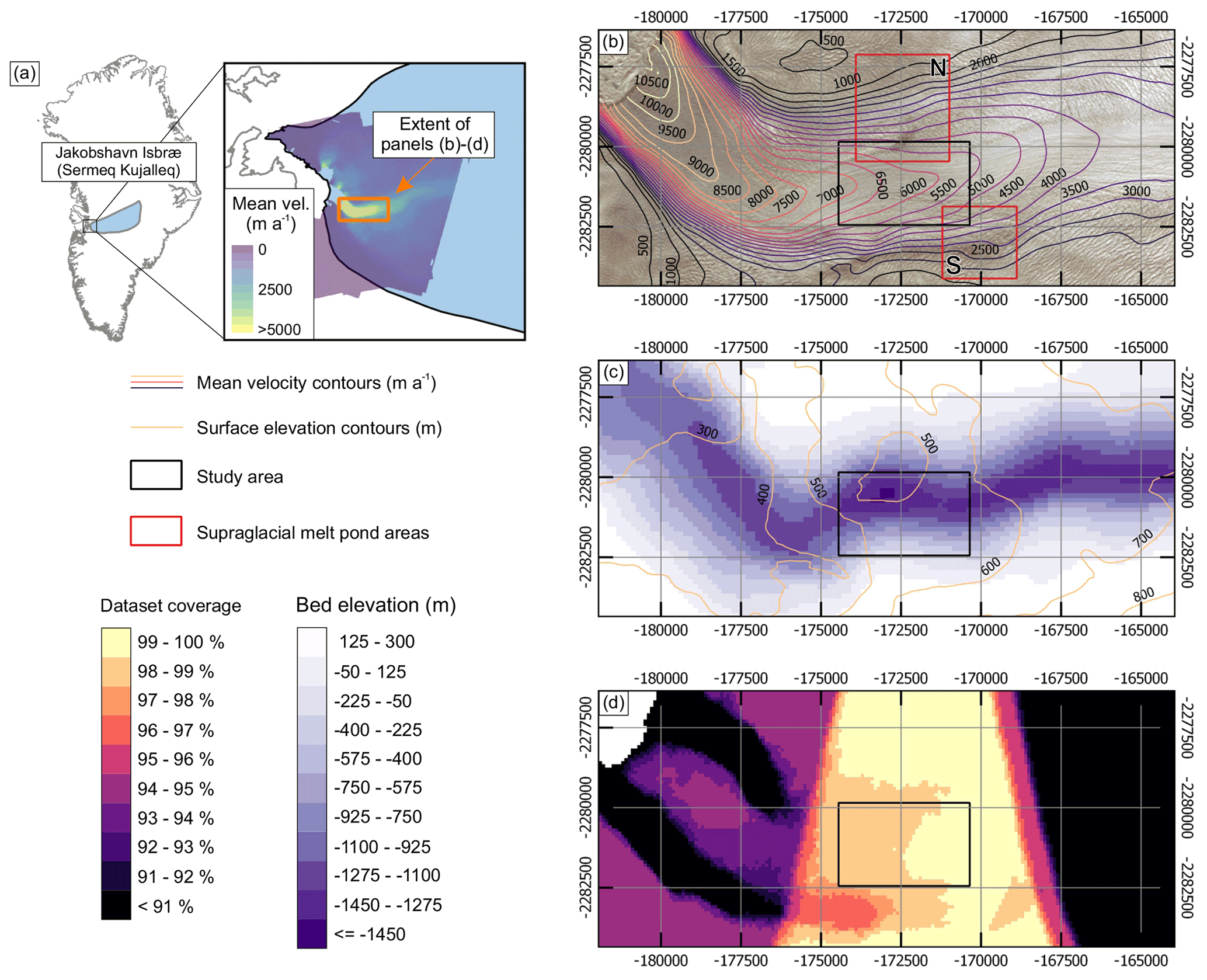
Figure 2 Summary of SK-JI and study area. (a) Location of SK-JI and mean velocity of “W69.10N” (Joughin et al., 2020b) v3 dataset. (b) Landsat image of the most retreated SK-JI position (September 2013), contours of the Joughin et al. (2020b) velocity dataset, study area of this study (black box), and the extent of the two boxes (red) used to characterise local meltwater pond behaviour. (c) Basal and surface topography (Morlighem et al., 2017). (d) Spatial coverage of SAR ice velocity dataset of Joughin et al. (2020b). Projection for (b–c) is epsg: 3413.

The ice velocity of this MEaSUREs sub-region is frequently measured with small image-pair separations and is therefore likely to capture the most complete range of glacier behaviour possible. Error associated with each pixel is approximately ± 10–20 m a⁻¹ but may be subject to geolocation errors up to 100 m, as outlined by Joughin et al. (2020a). We assign each velocity image the centre date from the image pairs used to derive it and record the image pair separation. In total 562 velocity magnitude images, and corresponding error maps, with centre dates from 17 June 2008 to 20 December 2019 were accessed.

From this dataset we select spatial and temporal limits in which the applicability of POD can be best assessed. Spatially, this selection is driven by data coverage as expressed on a pixel-by-pixel basis as a percentage of those 562 velocity images which contain a measurement (Fig. 2d). Riel et al. (2021) identified travelling waves in the trunk of SK-JI with a propagation speed of up to 400 m d⁻¹. To minimise the potential effect of this manifesting in POD modes and potentially limiting the identification of signals due to subglacial hydrology, we further limit our study to a 4 km long section such that any travelling wave within an 11 d image-pair velocity image will not be resolved. Furthermore, the travelling wave amplitude decreases sharply at 10 km from the terminus position (Riel et al., 2021, their Fig. 2), and so we seek to identify a region upstream of this. Temporally, this selection is driven by our requirement to identify a multi-year period in which fluctuations in velocity are primarily annual, in which no, or very little, multi-year trend is observed, and thus in which stationarity of the dataset is approached. We therefore select an exceptionally well sampled region of the SK-JI trunk (Fig. 2) and an analysis period of summer 2012 (1 June) to end of winter 2016 (1 March). The inter-annual velocity variability of SK-JI is strongly related to its terminus position (Lemos et al., 2018; Bondzio et al., 2017), and this period corresponds to a time of relatively stable frontal position with only a minor multi-year slowdown, contrasting to after 2016 when the rate of slowdown increases markedly (Lemos et al., 2018). Our study area contrasts to previous studies which have investigated the velocity of SK-JI with high temporal resolution at the near-terminus (Cassotto et al., 2015; Sundal et al., 2013). A total of 232 velocity images are available covering the study period and area, 229 of which have an image-pair separation of 11 d, two (centre dates: 7 August 2013; 9 June 2015) have a separation of 22 d, and one (centre date: 1 August 2013) has a separation of 33 d. The median difference between velocity image centre dates is 5 d, the 25th percentile 1 d, and the 75th percentile 10 d.

2.2.2 Data processing and POD

We prepare the dataset by reading in each ice velocity raster and saving a “stack” of colocated images, as well as a table of relevant metadata including raw filename, image pair dates, separation, and centre dates. In MATLAB R2020a the $i-j-t$ stack is then rearranged into the form of X (Eq. 1). Some small gaps exist in the satellite-derived velocity data, in the very southwest corner of our study area four measurements are missing in the pixel time series, and over the vast majority of the study area only one measurement is missing. To fill in these minor gaps we interpolate temporally the satellite-derived ice velocity measurements using D'Errico (2020). We then resample the velocity measurements using a piecewise, non-overshooting cubic interpolation (Akima spline) to be regularly spaced according to the median measurement gap (5 d). A SVD of this matrix is then calculated and a three-value moving average taken of rows of V to dampen very high-frequency fluctuations, following the best practice of Higham et al. (2016). These fluctuations are potentially due to some measured velocities being derived from image pairs closely spaced in time but collected with ascending and descending orbits, noted to result in velocity discrepancies in some areas by Riel et al. (2021). The velocity matrix is then reconstructed (i.e. the inverse of Eq. 1), and the mean of each pixel time series subtracted to find the velocity anomaly of the whole dataset. The POD is then performed as in Sect. 2.1 and Fig. 1. A MATLAB script for this procedure is provided with this paper.

2.3 Characterisation of surface hydrology

To test whether melt-season velocity fluctuations can be attributed to surface-to-bed glacial hydrology, as in Mair et al. (2002), we use satellite imagery within Google Earth Engine to characterise daily supraglacial meltwater pond behaviour. We focus on two immediately upstream sub-regions (Fig. 2) where ponds form quasi-annually. These correspond to the “saturated crevasses” CV2 and CV5 identified by Lampkin et al. (2013) as forming in 2007 and delivering enough meltwater during drainage to enhance basal sliding in a distributed subglacial hydrological system. We assume that rapid changes in ponded water extent correspond to spatially and temporally focussed delivery of meltwater to the ice bed.

To begin, we derive outlines of the maximum annual supraglacial melt pond extent for the melt season (1 May to 30 September, 2009–2019) from daily Moderate Resolution Imaging Spectroradiometer (MODIS) Terra images within Google Earth Engine (Gorelick et al., 2017). Level-2 MOD09GQ band 1 surface-reflectance data (250 m resolution) were cloud masked where coincident band 7 (500 m resolution resampled to 250 m resolution) reflectance values exceeded 0.09. Supraglacial melt ponds were defined using a dynamic threshold approach (Selmes et al., 2011; Williamson et al., 2017), in which a central pixel's value had a reflectance of less than 0.65 against the mean reflectance within a moving 21-by-21 pixel window.

These daily supraglacial melt pond area masks were subsequently summed to create annual composites of maximum melt pond extent, and false positives were removed where the ponded water either did not appear twice within 6 successive days from first appearance, was not observed during a period of 5 cloud-free days before the third occurrence, did not appear on three or more occasions over the melt season, or was observed on more than 50 % of cloud free days, acting to remove land or protruding bedrock (Cooley and Christoffersen, 2017; Liang et al., 2012).

We then create the two study areas around the maximum melt pond extents of 2009–2019 for high-resolution temporal analysis (Fig. 2b). Here we analyse daily MODIS imagery within these two subregions using the thresholding method above, recording the cloud cover and the “melt pond” area within each box. Importantly, we are unable to perform the same stringent quality control procedures on the daily record as on the annual record as it is limited by cloud cover and, potentially, shadows due to the rough crevassed terrain. We reject all measurements when cloud cover over each subregion is >10 %. We identify potential drainages qualitatively when no melt pond area is consistently detected after a period of consistent melt pond detection. Comparison of these dates with available corresponding 30 m spatial resolution Landsat-7 and Landsat-8 imagery demonstrates we accurately bracket major melt pond drainage events (Appendix A).

In addition to the remote sensing approach outlined above, we use runoff output from the Modèle Atmosphérique Régional (MAR) v3.11 (ftp://ftp.climato.be/fettweis/MAR/, last access: 2 April 2020) extracted from the SK-JI catchment (Mouginot and Rignot, 2019) and portioned into 500 m elevation bands using the dataset's surface height layer to characterise the seasonal runoff in, and upstream, of our study region.

2.4 Ancillary data

We draw upon several open datasets to aid interpretation of POD results: dates where rigid melange is present in front of SK-JI and its relative terminus position from Joughin et al. (2020b), and topographic datasets from BedMachine v3 (Morlighem et al., 2017). From these topographic datasets we estimate the subglacial water flow paths by calculating subglacial flow accumulations (using Schwanghart and Scherler, 2014) from the Shreve (1972) hydraulic potential surface where ice-bed effective pressure is zero. In our study area subglacial flow paths are strongly constrained by subglacial topography, nevertheless we also calculate Shreve flow paths with varying subglacial water pressures (ρ_w), expressed as a fraction of ice overburden (ρ_i) following Wright et al. (2016). We find subglacial water confluences and flow paths do not show major changes unless ${\mathit{\rho }}_{\mathrm{w}}/{\mathit{\rho }}_{\mathrm{i}}<\mathrm{0.5}$; such extreme low values are not observed in the boreholes of Wright et al. (2016), and as such we consider our simple modelling of flow paths robust and appropriate for this area.

3 Results and interpretation

3.1 POD

The decomposed dataset is shown in Fig. 3. The spatial weighting of Mode 1 broadly reflects the mean ice velocity pattern (Fig. 3b), and its temporal coefficient peaks annually in late summer and reaches its minimum in spring. This is confirmed by the power spectral density (Fig. 3c) showing an almost exclusive annual periodicity. The autocorrelation of Mode 1 results in an integral length scale of 20 image stack time steps, confirming that for our purposes this dataset is fully converged following the criterion of Tropea et al. (2007). There is no negative spatial weighting, meaning the entire study area increases (spring to summer) and decreases (autumn and winter) in phase, with a higher seasonal amplitude in the downstream of the study area.

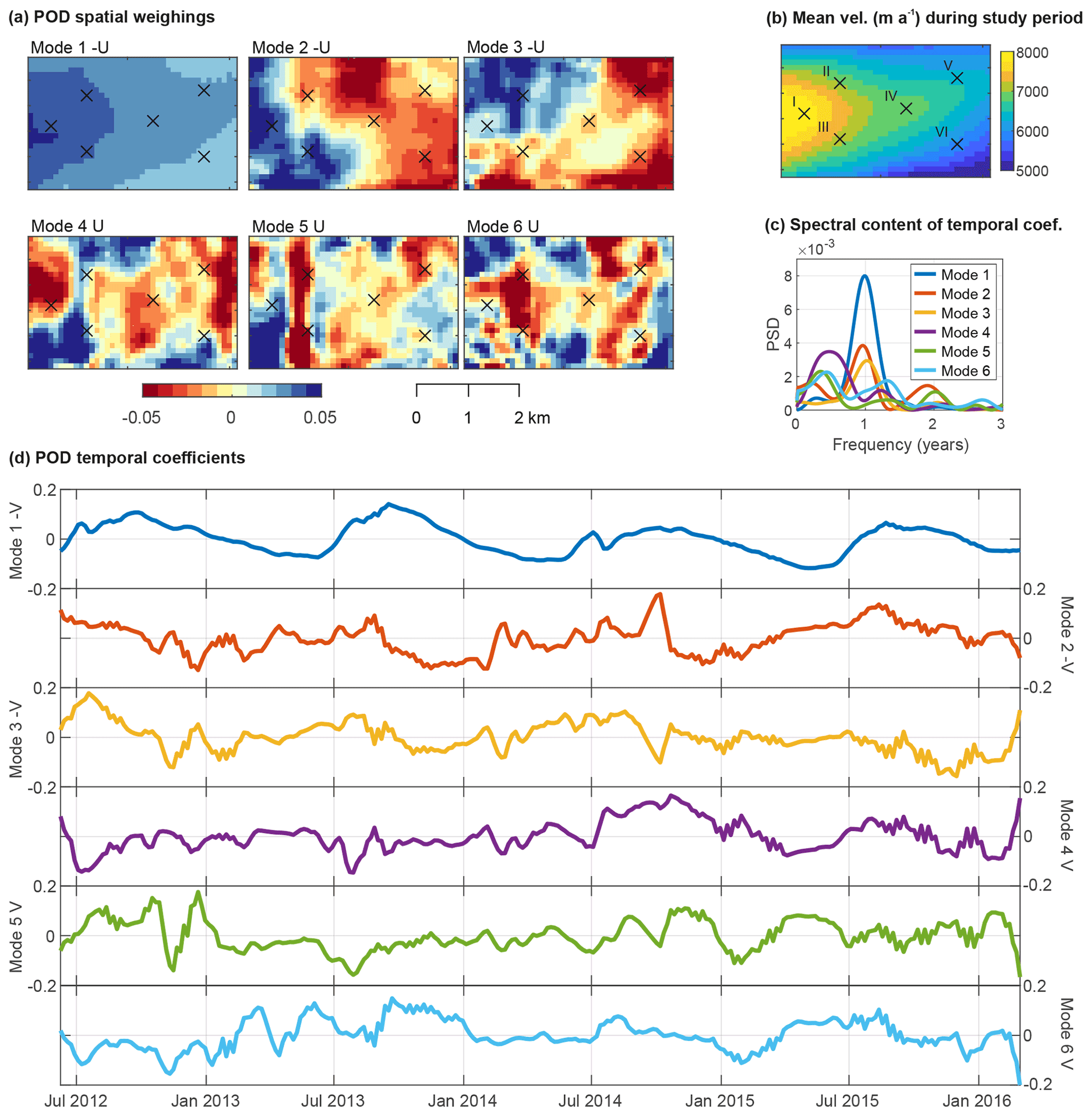
Figure 3 (a) The spatial weightings U for Modes 1–6. (b) Mean velocity of decomposed dataset and locations of representative points discussed later in this paper. Note that this is overall higher than the mean of the whole SAR-derived dataset, which is not resampled, and includes years of lower average velocity. (c) Power spectral density, or PSD, of the POD temporal coefficients. (d) The temporal coefficients, V, for Modes 1–6. To aid the interpretation of seasonality the sign ($+/-$) of Modes 1–3 are reversed such that V peaks in summer, and because this is applied to both U and V, this has no effect on the results.

Modes 2 and 3 show similar spatial structures with positive weighting to the west (down-glacier) of the study area and negative weighting to the east of the study area (up-glacier). This indicates a switching velocity differential across our study area, in which one area shows above average velocities due to this mode, while another shows below average velocities. Their temporal coefficients show annual periodicity and, generally, peak temporally in summer and have troughs during winter. Importantly, the temporal coefficients resemble quasi-conjugate pairs in that they have similar Var(%) values, and higher-frequency components appear mirrored in one another, for example, during the series of peaks in winter 2012 to spring 2013 and the major signal excursion in autumn 2014. Higham et al. (2018) showed that similar modal pairs in decomposed particle image velocimetry datasets relate to the formation of the von Karmen street in the lee of a flow obstacle. This indicates a common, but spatially variable or moving, process is responsible for Modes 2 and 3 in our dataset. When summed, these quasi-conjugate pairs may provide a picture of the overall distribution of the process responsible, and we investigate this further during POD interpretation (Sect. 3.2).

Modes 4 and 5 show some common spatial structures but no clear periodicity. Broadly spatial weightings are negative in the central east–west axis of the study area and negative towards the study area margins. The most prominent feature is the north–south narrow band of very high absolute values to the west of the study area. Mode 6 and lower modes show no discernible spatial structure either temporally or spatially, and they account for a very small amount of the dataset variance.

In Fig. 4 we plot the percentage of variance explained by each mode, calculated from the decomposition singular values. As expected, the variance is strongly dominated by Mode 1 (Var(%) =98.1). When plotted on a logarithmic axis, we see a distinct “kink” at Modes 2 (Var(%) =0.9) and 3 (Var(%) =0.5), which disrupts the otherwise smooth decay of eigenvalues characteristic of incoherent signals and noise in the higher modes. This is evidence that Modes 2 and 3 contain some physically meaningful information and that they are paired in some manner and warrant further investigation.

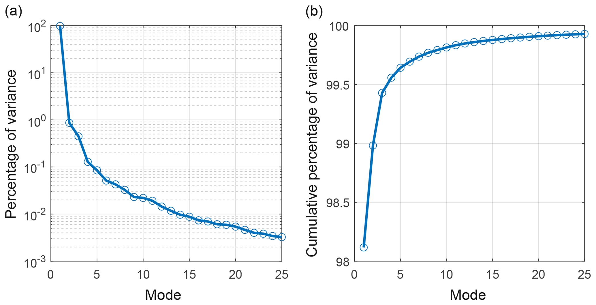
Figure 4 Plot of the percentage variance, Var(%), explained by each mode as calculated from Eq. (5) on (a) logarithmic and (b) cumulative scales.

3.2 Interpretation

The modes extracted from the decomposed dataset are purely statistical features and do not necessarily bear any relation to glaciological processes. In this subsection we compare the spatial modes and temporal coefficients with complementary glaciological and environmental datasets to assess whether the forcing from particular glaciological and environmental processes may contribute to the patterns revealed by the POD analyses. With this approach we explicitly do not assign glaciological meaning to the short wavelength features in the spatial modal weighting, U. This is important following our initial observation that Modes 2 and 3 appear paired and as such must be combined before any inference of broad forcing mechanism can be made. We also discuss the published errors of the original ice velocity dataset to ensure that we do not attach unwarranted glaciological significance to features in the decomposed dataset.

3.2.1 Glaciological and environmental factors

In Fig. 5 we compare the temporal coefficients (V; Fig. 5a) with a variety of potential glaciological forcing mechanisms. Mode 1 has a strong seasonal cycle that tracks the advance and retreat of the terminus position (Fig. 5e), following the increase in seasonal velocity amplitude observed in 2012 and 2013, before starting to decrease (Lemos et al., 2018). The peak value of the coefficient in each year coincides with the minimum terminus position in late summer. Annual peaks occur on 26 September 2012, 16 September 2013, 6 October 2014, and 22 August 2015. Even small fluctuations in the terminus position are reflected in Mode 1-V; for example, in mid December 2012 and late August 2015 short-term retreats in terminus position correspond with small positive deflections in Mode 1-V. Mode 1 does lag slightly behind terminus position change (Fig. 5e) – likely the adjustment time for the stress perturbation to reach our upstream study area. This supports an interpretation that Mode 1 reflects the dynamic enhancement and adjustment due to the changes in terminus stress associated with variations in calving or grounding line position. This physical interpretation of Mode 1 explains its dominance (Var(%) =98.1) and the increase in the positive spatial weighting in the direction of the calving terminus. This is expected as several other authors have also noted that stress reconfiguration due to frontal ablation dominates the bulk velocity signal of SK-JI (e.g. Joughin et al., 2020a; Khazendar et al., 2019; Lemos et al., 2018; Bondzio et al., 2017). Figure 6 shows two distinct, secondary, early summer peaks in the velocity at Points I–VI (most obvious in 2012 and 2014) also reflected in Mode 1. The causes of these peaks are not simply attributable to terminus position change or any forcing mechanism. Both occur in the highest 2 melt years and so may be due to meltwater input. That these are in Mode 1 indicates a widespread decoupling of the bed due to early season melting and subsequent pressurisation of the subglacial hydrological system, similar to “spring events” first seen on valley glaciers (Mair et al., 2003; Iken et al., 1983).

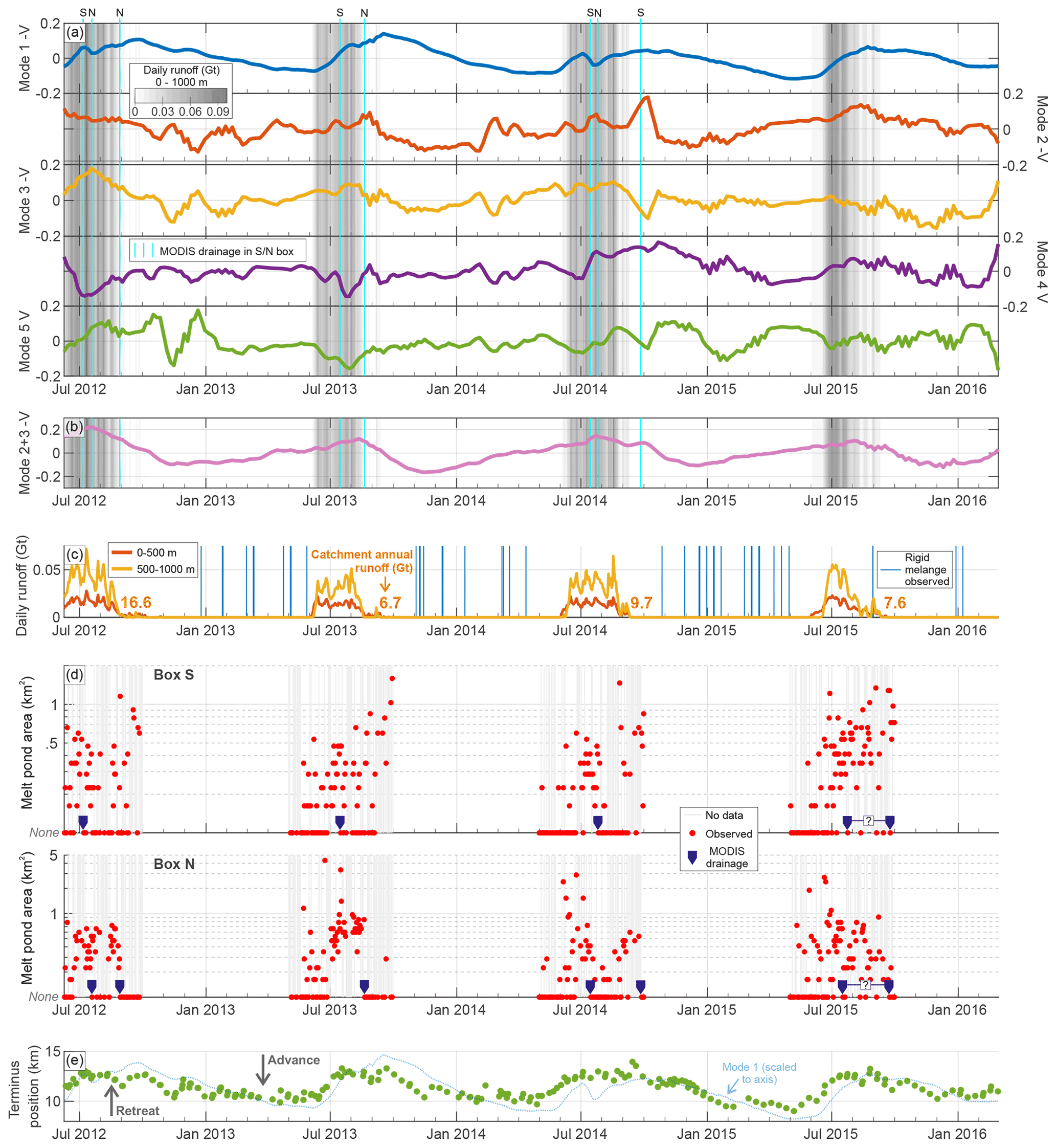
Figure 5 Temporal comparison of POD modes and environmental forcing. (a) Temporal coefficients, V, of Modes 1–5, which show some identifiable temporal or spatial coherence. Shading is level of runoff (see panel c), and light blue lines indicate potential supraglacial melt point drainages (see panel d). (b) V of Modes 2 and 3 summed showing a strong seasonal underlying process that peaks in the mid–late runoff period. (c) Runoff output from MAR v3.11 (ftp://ftp.climato.be/fettweis/MAR/, last access: 2 April 2020) for two elevation bands and for the total catchment; blue bars indicate observed periods of rigid melange following Joughin et al. (2020b). (d) Area of box S and N (Fig. 2b) covered by a melt pond and where rapid and consistent drops in meltwater area are interpreted as melt pond drainages; grey bars denote rejected data impacted by cloud cover (see Sect. 2.3). (e) SK-JI terminus position from Joughin et al. (2020b) with higher (lower) values indicating a more retreated (advanced) position; for illustrative purposes Mode 1-V is scaled and overlain.

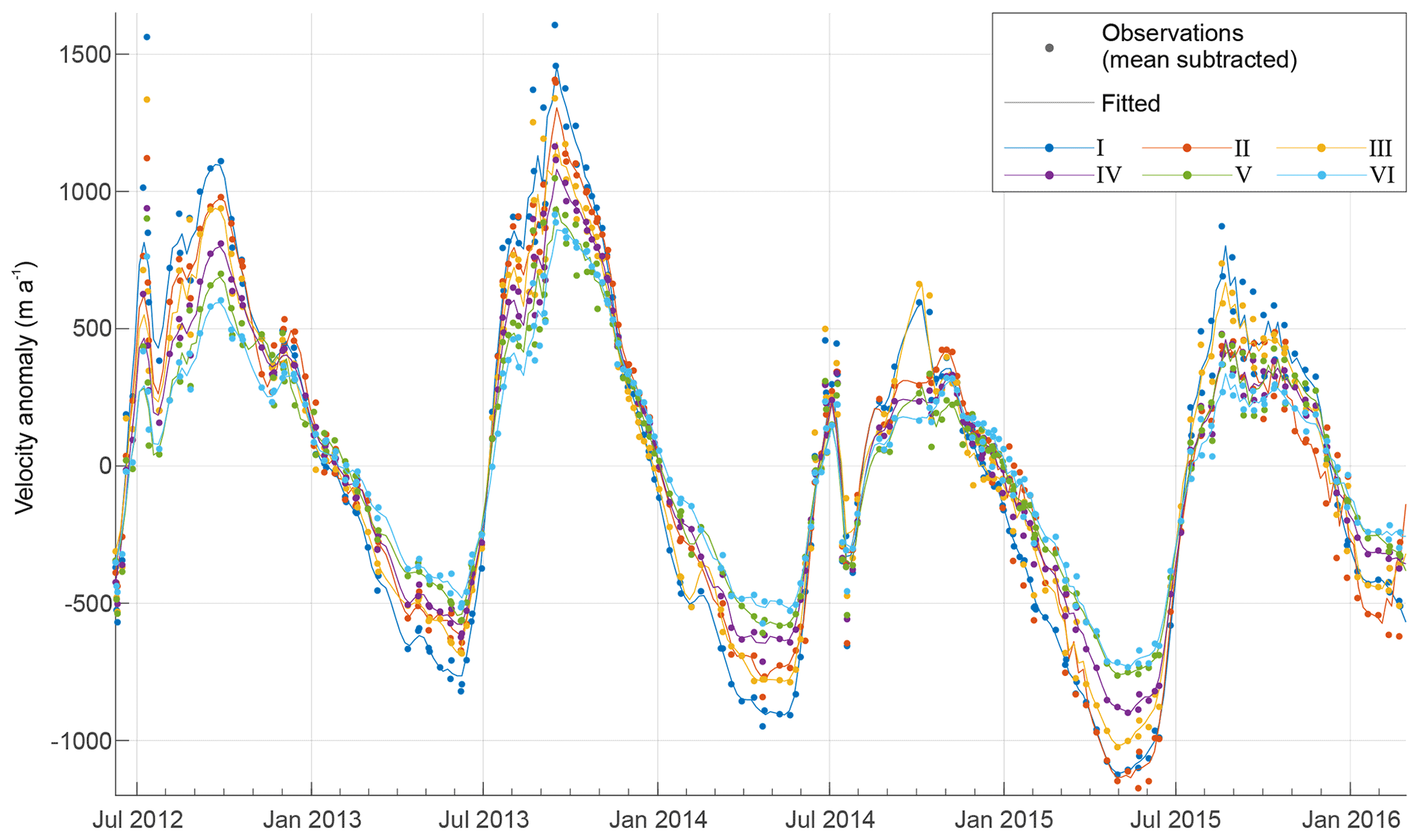
Figure 6 Measured and resampled velocity anomaly time series at Points I–VI referred to in Fig. 3.

Following from our interpretation that Modes 2 and 3 are quasi-conjugate pairs, i.e. that they are strongly related by a common process but with features shifted in phase, in Fig. 5b we sum Modes 2 and 3 (herein referred to as Mode 2+3) to gain an overall picture of the timing of the process responsible. Higham et al. (2018) discuss the occurrence of paired modes in the POD of natural flows in detail. The pattern of Mode 2+3 is strongly seasonal indicating that it is due to a recurrent glaciological process. The timing of the seasonality contrasts with Mode 1, however, with Mode 2+3 peaking on 18 July 2012, 12 August 2013, 23 July 2014, and 2 August 2015, meaning Mode 2+3 peaks, on average, 50 d before Mode 1. Temporal coefficient, V, for Mode 2+3 is most positive during mid-summer when both localised and catchment-wide runoffs reach their highest values and when supraglacial drainage events occur. V is most negative in November/December. These patterns indicate that Mode 2+3 may be strongly influenced by dynamic responses to melt-induced, subglacial hydrological forcings. However, hydrological forcing is complex as it will reflect temporal and spatial variability in the following:

1. different dominant modes of delivery of meltwater to the bed (e.g. Colgan et al., 2011), i.e.

   • a.

     short-term, spatially focussed, stochastic injections of large volumes of meltwater resulting from and typically immediately down-glacier from supraglacial drainage events or large moulins, versus

   • b.

     temporally dampened, spatially distributed routing of catchment-wide melt, typically captured by crevasse fields and directed along subglacial pathways determined by subglacial hydraulic potential;

2. different dominant subglacial drainage system types (e.g. Andrews et al., 2014), i.e.

   • a.

     hydraulically efficient, channelised drainage systems predominantly experiencing low water pressures, versus

   • b.

     hydraulically inefficient, distributed drainage systems predominantly experiencing high water pressures.

In Fig. 6 we plot the point velocity series for each of the representative points (I–VI). The annual peak SAR-derived measurements are on 27 September 2012, 14 September 2013, 3 October 2014, and 18 August 2015, very closely matching the Mode 1 peaks on 26 September 2012, 16 September 2013, 6 October 2014, and 22 August 2015. On close inspection of Fig. 6 the mid-melt-season secondary peak is observable in 3 of the 4 years and occurs on 11 July 2012, 1 August 2013, and 26 June 2014, close to the Mode 2+3 peaks. This suggests Modes 2 and 3 are related to these features in the non-decomposed velocity record; however, as noted above, these mid-melt-season peaks are also partially represented in Mode 1, suggesting that each mode does not completely reflect distinct glaciological processes.

One powerful use of POD is the ability to reconstruct the dataset using only selected modes, allowing us to see the combined effect of Modes 2 and 3 on ice velocity. In Fig. 7a–c we compare Modes 2 and 3 U, as well as the locations of persistent surface meltwater ponds and simple subglacial flow paths following Shreve (1972). In Fig. 7e the velocity due to Modes 2 and 3 is reconstructed at representative Points I–VI and compared to the temporal variation in supraglacial hydrology from Fig. 5. This approach offers a manageable way of interpreting the large POD result dataset in detail. Points I–VI were chosen to sample to the domain approximately evenly in space and prior to subsequent analysis. The significance of this lies not in explaining the detail of temporal and spatial glacier dynamics within a relatively small area, but rather lies in assessing the extent to which the POD modes are capable of discerning hydrological forcings, even on a glacier where glacier geometry, mass balance regime, and calving processes are more dominant.

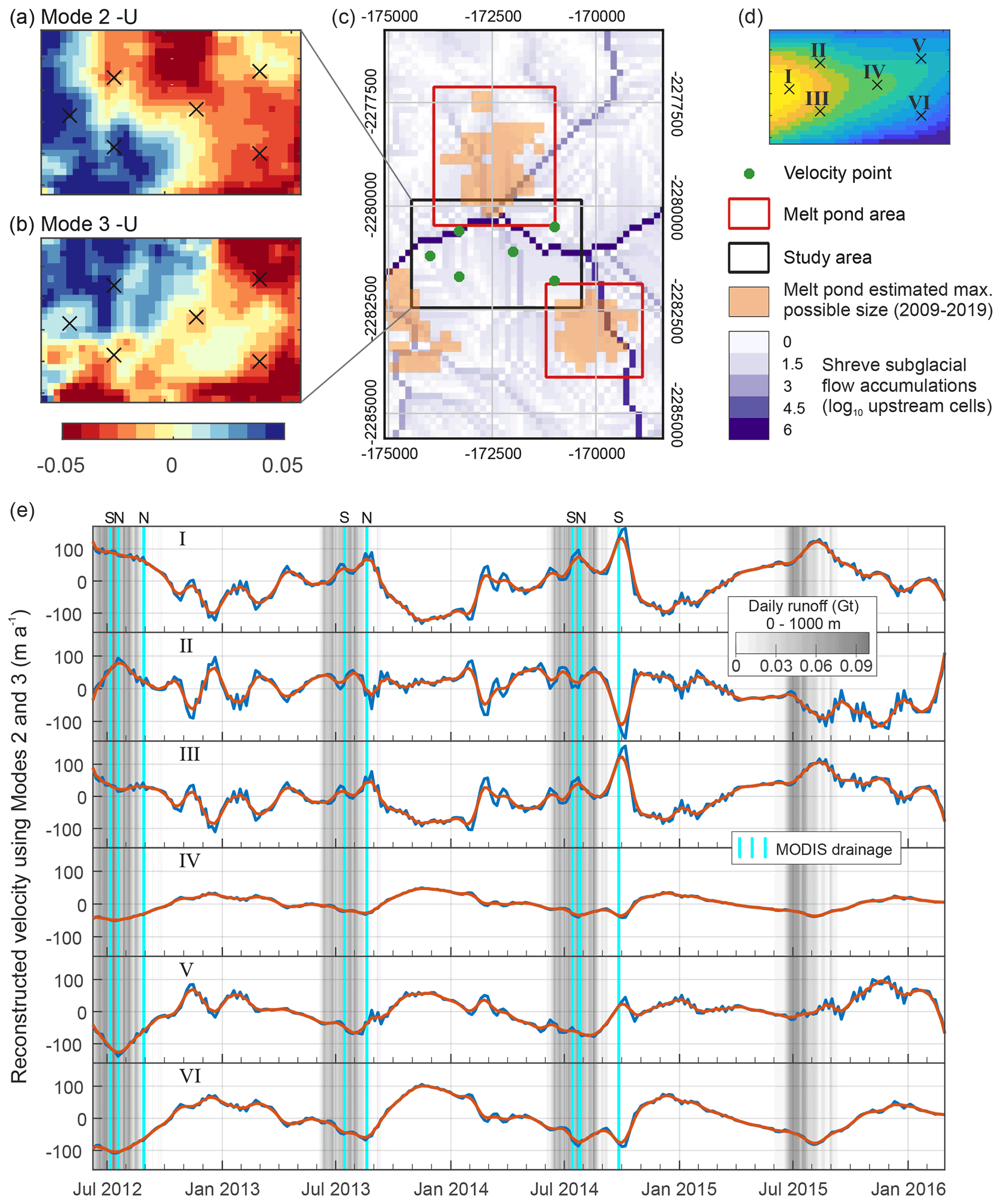
Figure 7 (a) Mode 2-U. (b) Mode 3-U. (c) Supraglacial melt pond locations and estimated subglacial hydrological routing (projection is epsg: 3413). (d) Representative point locations with mean SAR-derived velocity. (e) Comparison of reconstructed velocity from Modes 2 and 3, runoff and drainage displayed in (a) as in Fig. 5. Three-value (15 d) smoothed velocities are in orange.

We firstly discuss how different modes of delivery of water to the bed may influence the dynamic patterns revealed by Modes 2 and 3. Figure 7 reveals contrasting dynamic patterns between Points I–III, which display high-frequency variations superimposed on a broad annual cycle, and Points IV–VI, which show fewer high-frequency variations but a clearer annual cycle (Fig. 7e). Points I, II, and III are located down-glacier of all the supra-glacial melt ponds and are most proximal to the northern area, N, where the data indicate that ponded areas are larger and drainage events more frequent than the southern area, S (Figs. 5d, A1). Consequently, these locations will be most influenced by hydrological forcing as described in type 1a above which would explain pronounced fluctuations in velocity anomalies, some of which are clearly coincident with identifiable meltwater drainage events. Points IV–VI display less short-term velocity variability as they sit downstream of the less active area S. The different locations also vary in the sign of their dynamic response to potential melt pond drainage events, as identified in Fig. 5d. For example, Points I and III show an increase in velocity coincident with potential drainage events, whilst Point II shows a decrease in velocity coincident with these events. To explain this and other patterns we secondly discuss how subglacial drainage system structure affects dynamics, invoking conceptual models of their spatial and temporal evolution.

Shreve's subglacial flow accumulations (Fig. 7c), derived from hydraulic equipotential mapping, indicate the likely preferential drainage axes (PDAs) within the study area. These are the broad axes along which temporally dampened, catchment-wide melt from up-glacier will be directed during summer (i.e. type 1b above) and where base-level water flow, generated from frictional melting, will flow throughout the year. Bearing in mind that, in this region, subglacial flow paths are strongly constrained by topography (Sect. 2.4), we are cautious to not over-interpret their precise location and refer to reconstructed PDAs in conjunction with other independent data sources. Furthermore, uncertainties in basal topography create uncertainties in the exact locations of PDAs (MacKie et al., 2021); hence in areas where multiple PDAs are confluent, we have higher confidence that these are areas of high hydrological activity. Shorter-term dynamism and transients will undoubtably result in subglacial flow paths outside of these axes (Stevens et al., 2018; Wright et al., 2016), but given that the velocity dataset analysed here are 11 d image pairs, we would be unlikely to be able to resolve any such higher-temporal- and higher-spatial-resolution hydro-dynamic coupling. The dynamic response to hydrological forcing will vary through time as the drainage system evolves. Following Röthlisberger (1972), when discharge through these regions is consistently high (as would be likely during the summer melt season), turbulent flow will develop which may result in the development of hydraulically efficient, possibly channelised, low-pressure subglacial flow (i.e. type 2a above) with minimal impact on basal sliding and ice velocity. This would explain why Points IV, V, and VI, which are located close to major confluences in flow accumulation, show negative velocity anomalies during the summer melt seasons. The development of efficient drainage at Point II (located directly over a PDA) also explains the negative velocity anomalies during drainage lake drainage events, as noted above. Conversely, during the rest of the year, all drainage axes will have closed by ice deformation, and the glacier will likely be underlain by an inefficient, distributed drainage system (i.e. type 2b above). During these periods, the areas with confluent PDAs will become the most likely areas of the bed to experience low-magnitude, base-level water flows which will promote higher water pressures and enhanced basal sliding. Consequently, Points IV, V, and VI show positive velocity anomalies during the winter. The annual cycle of Points I and III shows negative velocity anomalies during the winter which likely reflects their isolation from flow confluences and hence that they are likely to be located over unconnected regions of the glacier bed where there is minimal hydrological forcing in the winter (following Hoffman et al., 2016). In summer, the forcings from high-magnitude melt pond drainage events discussed above create positive velocity anomalies at Points I and III since short-term, high-magnitude discharge is forced into inefficient drainage systems, hence provoking high basal water pressures. Notable fluctuations in velocity seen at Points I–III in December 2012 may be due to release of stored water from englacial or subglacial sources (Pitcher et al., 2020).

Despite the complex temporal and spatial modal patterns described by Modes 2 and 3 we propose that together these modes do define the component of dynamic variability that is strongly influenced by changing patterns of subglacial hydrological forcings. The seemingly complex behaviour can be explained with recourse to long-standing hydrological theory and simple conceptual models for meltwater delivery mechanisms and drainage system structures. If the POD analyses could be performed over a larger spatial scale, or across a glacier that was less directly dominated by calving dynamics, then POD modes might be defined that more obviously reflect subglacial hydrological forcing, similar to Mair et al. (2002). This will become possible as the temporal resolution and spatial extent of satellite-derived glacier and ice sheet dynamics continue to improve.

3.2.2 SAR-derived velocity error analysis

In this subsection we consider the published errors of the SAR velocity product of Joughin et al. (2020b) itself and their likely effect, if any, on our POD mode results. In our domain and study period the median error for individual pixels is 11–19 m a⁻¹, with maximum (minimum) values of 18–21 (5–10) m a⁻¹. Importantly, these values relate to the bulk, non-decomposed velocity record and not individual modal components of the velocity as identified with POD. The velocity fluctuations in the reconstructed velocity series using only Modes 2 and 3 (Fig. 7) vary by an order of magnitude more, typically from −100 to +100 m a⁻¹ with extreme values almost twice this. As such, even if we were to make the simplistic assumption that Modes 2 and 3 experience all the error, rather than some portion of it, our interpretation would remain unchanged. The time series of velocity error magnitudes at Points I–VI are highly variable measurement-to-measurement and do not show a seasonal pattern, unlike Modes 2 and 3. A relevant study of POD and measurement errors comes from Wang et al. (2015) who showed that errors in a particle image velocimetry dataset are accommodated in the higher-order modes, not the lower modes, due to physical processes. This study, along with the above discussion, lead us to conclude similar behaviour in this study. Nevertheless, to check the robustness of our decomposition, we create an “error envelope” for the reconstructed velocities of Modes 2 and 3 shown in Fig. 7. We do this by repeating the POD with the published error added to the velocity field and then with the error subtracted. This results in variations in the velocity anomalies shown in Fig. 7 of around ±1 m a⁻¹ which are negligible in the context of the velocity fluctuations due to Modes 2 and 3, as well as our interpretation that they are dominated by glacio-hydrological-induced ice motion.

3.2.3 Interpretation summary

To summarise, Mode 1 relates strongly to the terminus-driven variability that is known to strongly dictate the bulk observed velocity signal of SK-JI. Modes 2 and 3 together describe the seasonal development of the spatially variable subglacial hydrological system influenced by episodic input of meltwater and the changing efficiency of subglacial hydrological drainage axes. Mode 4 and lower modes show no interpretable spatial or temporal patterns and therefore likely do not contain useful statistical information.

4 Discussion

The work presented here is an important contribution to efforts to explain how patterns of ice motion, observed from space, can reveal different glaciological forcing mechanisms. As the outlet glaciers of Greenland retreat, and their geometry and flow evolves, it is likely that the relative importance of processes governing their ice dynamics will also evolve, though this is less easily assessed. This study acts as a proof of concept, building on the work described by Mair et al. (2002), that the eigen-decomposition of ice velocity can detect the influence of changes in glacial hydrology on ice dynamics. Figure 7 shows that hydrologically forced flow contributes to velocity variabilities of approximately ±100 m a⁻¹ to the ice flow in our study area of SK-JI. This contribution varies seasonally but also in response to sudden inputs of meltwater.

Our study area within SK-JI was chosen owing to the excellent and openly available ice velocity dataset, but it is arguably not the ideal place to test the applicability of POD to ice velocity due to the dominance of stress patterns created by changing terminus geometry on the overall seasonal velocity, as outlined by previous work (Joughin et al., 2020a; Lemos et al., 2018; Bondzio et al., 2017). The application of POD analyses to a velocity record from a marine-terminating glacier with seasonal behaviour more influenced by subglacial hydrology such as Kangiata Nunaata Sermia (e.g. Davison et al., 2020; Sole et al., 2011) or a land-terminating section of the ice sheet, especially one with complementary discharge measurements such as Russell and Leverett glaciers (e.g. Davison et al., 2019; Chandler et al., 2013), might yield more insights into their hydro-dynamic coupling behaviour. This underlines the importance of continued production of high-resolution, all-year SAR datasets of ice velocity in key, dynamic areas. Practically this involves the continued exploitation of Sentinel 1 and TerraSAR-X/TanDEM-X for ice velocity and, looking forward, to future missions such as NASA-ISRO SAR (NISAR).

In this analysis we only characterise supraglacial melt pond drainages in the immediate locality of our study area. We find, however, that the identified drainages appear to explain the major excursions in velocity reconstructed with Modes 2 and 3. At Sermeq Kujalleq (Store Gletsjer), the drainage of supraglacial lakes has been shown to rapidly increase the efficiency of the subglacial drainage system and decrease ice velocity at a point near the terminus (Howat et al., 2010), strengthening our interpretation in this study that the drainage of supraglacially ponded water can both slow and enhance ice velocity. The interpretation of decomposed surface velocity fields presents a potential method for comparing field data to model output in a more developed manner than straightforward correlations. We propose comparing low-dimensional representations of measured ice velocity (i.e. separated POD modes) with ice sheet model outputs calculated with differing parameterisations of subglacial hydrology and basal motion. This would provide a means of assessing the efficacy of models to account for spatially and temporally variable hydro-dynamic coupling, ultimately leading to more physically robust predictions of future ice sheet behaviour.

The POD technique applied here is complementary to that of Riel et al. (2021), who also decomposed the ice velocity record of SK-JI as imaged by TanDEM-X and TerraSAR-X from Joughin et al. (2020b, 2010). In that study the velocity time series of a wider area is decomposed into the seasonal cycle and transient multi-annual parts to show the propagation of a kinematic wave emanating from the glacier terminus. In this study we have isolated years when data stationarity can be reasonably argued, essentially removing the multi-annual transient. Consequently, our Mode 1, primarily due to seasonal terminus fluctuations, is broadly analogous to their seasonal velocity signal. Our Modes 2 and 3, which apparently relate to glaciohydrological processes, occur on shorter timescales than the seasonal signal extracted by Riel et al. (2021). Riel et al. (2021) show that their B-spline approach can be used to detrend multi-annual velocity variations. This raises the prospect of applying POD to the reconstructed seasonal velocity only. This could address the issue of stationarity that limits the applicability of POD to datasets with long-term trends, a common feature of ice velocity time series. One consideration that might complicate this, however, is that in the 4 years analysed in this study, the influence of subglacial hydrology appeared to be split into a set of quasi-conjugate pairs of modes (Sect. 3.1). Therefore, over a longer time period, one may expect that the influence of hydrological forcing on spatial patterns of ice motion may be divided across many more separate modes which would make physical interpretations more difficult. One factor to be considered in further use of POD is the length scales over which basal variability is transferred to the ice surface velocity and modal components of that surface velocity. This study, and Mair et al. (2002), offers empirical evidence that changes in basal hydrology are reflected in modal components of the velocity field on length scales close to the limit where “bridging stresses” might obscure the velocity response of basal hydrology had the bulk velocity signal been interpreted alone. Future work could investigate these effects further, potentially using POD to focus on key glaciological features (e.g. supraglacial lakes, subglacial lakes, patterns of basal drag, and/or ice stream sticky spots) over timescales and length scales that capture their dynamism.

5 Conclusions and outlook

In this study we have presented the first application of proper orthogonal decomposition (POD) to a series of satellite-derived maps of ice velocity. By focussing on an exceptionally well-sampled area of the SK-JI trunk from 2012–2016 (Joughin et al., 2020b), we significantly develop the POD/EOF analysis using survey stake observations of ice velocity on Haut Glacier d'Arolla by Mair et al. (2002) and apply it to a Greenlandic marine-terminating glacier.

We explored statistical structures or “modes” in the data that partially explain dataset variance. The first, Mode 1, clearly relates to the bulk velocity signal that previous researchers have shown links strongly to terminus-driven stress reconfiguration, transferred upstream rapidly due to low bed and lateral resistance (Joughin et al., 2020a; Bondzio et al., 2017). However, a second seasonal pattern exists which we hypothesise is due to glacio-hydrological processes. We present independent evidence from remote sensing and several published datasets to support this interpretation and explain the observations in terms of proximity to the confluences of subglacial preferential drainage axes and the input of meltwater to the subglacial environment from two nearby supraglacial melt ponds. Short-term dynamism of glaciers is often explained in the context of evolving subglacial drainage systems and with respect to the manner of water delivery to the bed. Our POD analysis offers a powerful means to disentangle such complex influences from other higher-order drivers of ice dynamics. The decomposed modes may contain some small artefacts that relate to the original dataset and its errors. Modes do not necessarily relate to a single glaciological process, and signals due to spatially variable processes may be split between modes. However, we have shown that with careful interpretation these effects can be accommodated for. As ice velocity measurements continue to increase in spatio-temporal resolution and continuity, these will likely reduce in the future.

POD and potentially related decomposition techniques such as dynamic mode decomposition (Schmid, 2010) are flexible, powerful, and quick techniques that can be applied to other colocated measurements of ice surface velocity, derived from satellites, time-lapse imagery, or GPS stake networks. The next step is to apply POD to other high-resolution records of ice surface velocity from glacier systems with a different balance of processes with contrasting propagation speeds. Where hydrology is a more important control on the overall velocity pattern, its associated modal expression would be more dominant. We have applied POD only to the ice velocity magnitude; however, extending the analysis to polar stereographic grid x and y components is relatively simple and may provide insights to explain ice velocity patterns in the vicinity of key glacio-hydrological features. Furthermore, POD may offer a low-dimensional method of comparing surface velocity measurements with coupled glacier hydrology and ice dynamics models that simulate hydrological and ice dynamic processes explicitly and coincidently. We assert that computationally lightweight modal decomposition techniques such as POD can become a key method in illuminating the effects of individual glacial processes on combined emergent patterns of ice dynamics.

Appendix A

To evaluate the results of the daily MODIS dynamic thresholding method as outlined in Sect. 2.3, we compare US Geological Survey Landsat-7 ETM+ band 4 and Landsat-8 OLI band 5 scenes with <30 % cloud cover either side of, and close to, the drainage dates detected using the daily MODIS thresholding method as shown in Fig. 5. This acts as a validation of the automated Google Earth Engine approach and a validation that the daily, but relatively low-resolution, MODIS can detect melt pond drainages in this setting. It is important to note that the time between identified drainage and a suitable Landsat-7/Landsat-8 image acquisition varies considerably, and this must be considered when comparing the two datasets. Furthermore, due to the large contrast in spatial resolution between MODIS (250 m) and Landsat-7 and Landsat-8 (30 m), we expect some disparity between the two approaches. The overall aim here is to increase confidence that the timing of the delivery of meltwater from the surface to englacial and ultimately the subglacial environment is correctly bracketed.

Figure A1 Satellite images of the south (S) and north (N) melt pond study regions, outlined in red (Fig. 1b). Pooled water is indicated by flat, black regions. Imagery from (a)–(j) is from Landsat-7 ETM+ band 4 (0.77–0.90 µm), and stripes of missing data are due to the well-known scan line corrector error. Imagery from (k)–(t) is from Landsat-8 OLI band 5 (0.85–0.88 µm). Dates of image acquisition are shown in panel title, and dates of drainages (Fig. 5) as identified through daily MODIS dynamic thresholding method (Sect. 2.3) are shown in table insert. Landsat-7 and Landsat-8 imagery is used courtesy of the US Geological Survey.

Results are shown in Fig. A1. In the less active southern melt pond area one drainage event is identified per year, occurring in July. For the 2012 and 2013 drainages, S1 and S2 in Fig. A1, the available images show a slightly smaller ponded area, indicating that only a partial drainage took place or refilling partially occurred in the days after drainage and before the Landsat acquisition. The 2013 drainage, S3, however is well identified by our technique. In 2012 and 2013 a secondary drainage (Fig.  A1c–d and A1j–k) takes place. These are visible in Fig. 5d as a short return to zero melt pond area conditions after short periods of consistent meltwater detection, but these were not judged to be clear enough for identification as a potential drainage event during analysis (Sect. 2.3). In both these cases, however, drainage corresponds closely to the drainage of the larger, more active northern melt pond area which is, in all cases, well-identified with the MODIS-derived record. In totality, this comparison increases our confidence in our approach to correctly identify melt water leaving the ice surface and, in turn, our interpretation that Modes 2 and 3 are strongly influenced by glacier hydrology.