the Creative Commons Attribution 4.0 License.
the Creative Commons Attribution 4.0 License.
 | 05 May 2022
Understanding monsoon controls on the energy and mass balance of glaciers in the Central and Eastern Himalaya
Catriona L. Fyffe
Simone Fatichi
Evan Miles
Michael McCarthy
Thomas E. Shaw
Baohong Ding
Wei Yang
Patrick Wagnon
Walter Immerzeel
Francesca Pellicciotti
The Indian and East Asian summer monsoons shape the melt and accumulation patterns of glaciers in High Mountain Asia in complex ways due to the interaction of persistent cloud cover, large temperature ranges, high atmospheric water content and high precipitation rates. Glacier energy- and mass-balance modelling using in situ measurements offers insights into the ways in which surface processes are shaped by climatic regimes. In this study, we use a full energy- and mass-balance model and seven on-glacier automatic weather station datasets from different parts of the Central and Eastern Himalaya to investigate how monsoon conditions influence the glacier surface energy and mass balance. In particular, we look at how debris-covered and debris-free glaciers respond differently to monsoonal conditions. The radiation budget primarily controls the melt of clean-ice glaciers, but turbulent fluxes play an important role in modulating the melt energy on debris-covered glaciers. The sensible heat flux decreases during core monsoon, but the latent heat flux cools the surface due to evaporation of liquid water. This interplay of radiative and turbulent fluxes causes debris-covered glacier melt rates to stay almost constant through the different phases of the monsoon. Ice melt under thin debris, on the other hand, is amplified by both the dark surface and the turbulent fluxes, which intensify melt during monsoon through surface heating and condensation. Pre-monsoon snow cover can considerably delay melt onset and have a strong impact on the seasonal mass balance. Intermittent monsoon snow cover lowers the melt rates at high elevation. This work is fundamental to the understanding of the present and future Himalayan cryosphere and water budget, while informing and motivating further glacier- and catchment-scale research using process-based models.
- Article
(3591 KB) - Full-text XML
-
Supplement
(1551 KB) - BibTeX
- EndNote


High Mountain Asia (HMA) holds the largest ice volume outside the polar regions (Farinotti et al., 2019) and due to the large elevation range and vast geographic extent, HMA glaciers are highly diverse in character and hydro-climatic context (Yao et al., 2012). Several large-scale weather patterns interact with the region's topography (Bookhagen and Burbank, 2010), causing glaciers to contrast in terms of hypsometry (Scherler et al., 2011a) and accumulation and ablation seasonality (Maussion et al., 2014). The Indian Summer Monsoon dominates the Central Himalaya and the southeastern Tibetan Plateau during summer, and gradually loses strength moving towards the Karakoram, Pamir and Kunlun ranges in the west, where the influence of westerlies is particularly strong. A more continental regime, influenced by both monsoon and westerlies, controls the Central Tibetan Plateau (Yao et al., 2012; Mölg et al., 2014), while the East Asia Monsoon influences the eastern slopes of the Tibetan Plateau (Yao et al., 2012; Maussion et al., 2014). These major modes of atmospheric circulation control the surface processes and runoff regimes of glaciers (e.g. Kaser et al., 2010; Mölg et al., 2012, 2014) and lead to distinct responses of glaciers to climate change (Scherler et al., 2011b; Yao et al., 2012; Sakai and Fujita, 2017; Kraaijenbrink et al., 2017). Mass losses are high throughout most of HMA, and are particularly pronounced on the southeastern Tibetan Plateau, while glaciers exhibit a near-neutral mass-balance regime throughout the Karakoram, Pamir and Kun Lun (Gardelle et al., 2012; Brun et al., 2017; Farinotti et al., 2020; Shean et al., 2020).
Accurate glacier mass-balance modelling is essential for assessing glacier meltwater contribution to mountain water resources, and for predicting future glacier states and catchment runoff. Physically based models of glacier energy and mass balance represent surface and subsurface energy fluxes using physical equations to calculate the energy available for melt and the glacier runoff. Summer-accumulation glaciers in HMA experience simultaneous accumulation and ablation. Using an energy-balance model, Fujita and Ageta (2000) found that the mass balances of this type of glacier is highly sensitive to climatic variability during the monsoon season, when warm air temperatures and high precipitation rates coincide. Using energy-balance modelling for an interannual study at the Central Tibetan Zhadang glacier, Mölg et al. (2012) demonstrated that the timing of monsoon onset and the associated albedo variability can change melt rates considerably in subsequent years. At the same time, they observed a decoupling of the glacier mass balance from the Indian Summer Monsoon during the main monsoon season. Mölg et al. (2014) explain the mass-balance variability of the Zhadang Glacier as being controlled by both the Indian Summer Monsoon onset and mid-latitude westerlies. Combining energy balance with weather forecast modelling, Bonekamp et al. (2019) identify the timing and quantity of snowfalls as the main source of differences in mass-balance regimes between the Shimshal Valley in the Karakoram and the Langtang Valley in the Central Himalaya. Similarly, Zhu et al. (2018) attribute mass-balance differences of three glaciers on the Tibetan Plateau mainly to different local rain/snow precipitation ratios and timing.
The presence of debris cover, a widespread characteristic of HMA glaciers, (e.g. Scherler et al., 2011b; Kraaijenbrink et al., 2017; Herreid and Pellicciotti, 2020), adds additional complexity to understanding and modelling the processes leading to (sub-debris) glacier melt. In recent years, much effort has gone into developing energy-balance models for debris-covered glaciers (e.g. Nicholson and Benn, 2006; Reid and Brock, 2010; Lejeune et al., 2013; Fujita and Sakai, 2014; Collier et al., 2014; Rounce et al., 2015; Evatt et al., 2015; Steiner et al., 2018). Yang et al. (2017) compared the energy balance of a debris-covered and a clean-ice glacier on the southeastern Tibetan Plateau and found the main differences, beside the differences in melt rates, is their climatic sensitivity and the important role of turbulent fluxes on debris-covered glaciers. Studies with observational data on two Indian glaciers showed that thick debris is a more important control on melt rates than elevation (Pratap et al., 2015; Shah et al., 2019) and it also dampens and delays glacier melt in the diurnal cycle (Shrestha et al., 2020). Ablation is often expected to be higher on glaciers with debris around or below the critical thickness (site dependent, 1–5 cm) (Nakawo and Rana, 1999) than both at clean-ice sites and at sites with thicker debris cover, as shown experimentally (Östrem, 1959; Reznichenko et al., 2010) and by means of modelling (e.g. Nakawo and Rana, 1999; Reid and Brock, 2010), with humidity being a determining factor for this enhancement (Evatt et al., 2015). Moisture in debris is an important factor under monsoonal conditions, controlling the debris thermal properties and thus ablation (Sakai et al., 2004; Nicholson and Benn, 2006) and has been the focus of dedicated modelling studies (Collier et al., 2014; Giese et al., 2020). Moreover, the representation of latent heat due to evaporation (Steiner et al., 2018; Giese et al., 2020) and atmospheric stability correction for turbulent fluxes were shown to be important for improving the simulation of sub-debris melt (Reid and Brock, 2010; Mölg et al., 2012). Previous studies explicitly dealing with the imprint of the monsoon on the surface thermal properties of glaciers remained limited to individual clean-ice glaciers in the Central Tibetan Plateau (Mölg et al., 2012, 2014).
Our main goal is to improve the understanding of monsoon controls on glaciers of various surface types in the Central and Eastern Himalaya. Applying the glacier energy- and mass-balance module of a land surface model suited to both debris-covered and clean-ice glaciers, and leveraging seven on-glacier automatic weather station (AWS) records from the region, we answer the following questions: (1) Which energy and mass fluxes dominate the seasonal mass balance of Himalayan glaciers? (2) How does debris cover modulate the energy balance in comparison with clean-ice surfaces? (3) How does the monsoon change the glacier surface energy balance? Answering these questions allows us to infer how these glaciers will respond to the possible future changes of the monsoons in the region. We apply the model at the point scale of individual AWSs, driven by high-quality in situ meteorological observations that guarantee accurate energy-balance simulations, not affected by extrapolation of the meteorological forcing. By identifying the key surface processes of glaciers and their dynamics under monsoonal conditions, this study promotes their appropriate representation in models of glacier mass balance and the hydrology of glacierised catchments.
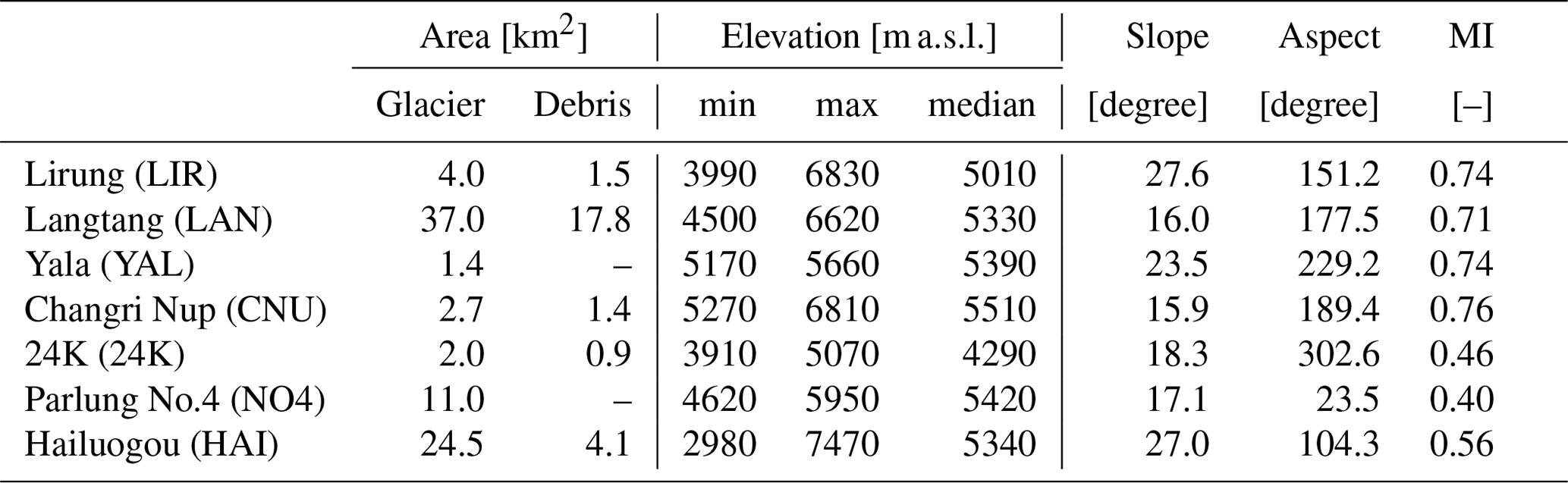
In situ observations from seven on-glacier AWSs in different environments along the climatic gradient of the Himalaya were gathered and used for forcing and evaluation of the model (Fig. 1 and Table 1). Our study sites are located in the Central and Eastern Himalaya and cover a range of glacier types and local climates (Figs. 1, 2 and Table 2). The seven sites include both spring- (24K, Parlung No.4) and summer-accumulation glaciers (all others) as indicated by the proportion of monsoon precipitation to the annual precipitation (Fig. S1 in the Supplement). Langtang, Lirung and Yala are neighbouring glaciers found in the Langtang Valley (Fig. 1). The Langtang Valley is strongly influenced by the Indian Summer Monsoon (∼ June to October), during which more than 70 % of the annual precipitation occurs (Fig. S1 and Table 2), while the period from November to May is a drier season (Immerzeel et al., 2012; Collier and Immerzeel, 2015). The valley has been a site of extensive glaciological (e.g. Fujita et al., 1998; Stumm et al., 2020), meteorological (Immerzeel et al., 2014; Collier and Immerzeel, 2015; Heynen et al., 2016; Steiner and Pellicciotti, 2016; Bonekamp et al., 2019) and hydrological (e.g. Ragettli et al., 2015) investigations. On-glacier AWSs were installed during the ablation season on Lirung (2012–2015) and Langtang (2019) glaciers, and year-round on Yala (2012–ongoing) (Table 1). Both Lirung and Langtang are valley glaciers that have heavily debris-covered tongues, but the tongue of Lirung has disconnected from the accumulation zone (Fig. 2). Yala is a considerably smaller clean-ice glacier, with most of its ice mass located at comparably high elevation. It is oriented to the southwest and has a gentle slope (Fujita et al., 1998) (Fig. 2 and Table 2).
North Changri Nup Glacier (hereafter Changri Nup Glacier) is a debris-covered valley glacier located in the Everest region in Nepal (Fig. 1). The southeast-oriented, avalanche-fed glacier discharges into the Koshi River system. The local climate is similar to that of the Langtang Valley, with 70 %–80 % of precipitation falling during monsoon (Vincent et al., 2016) (Figs. 2, S1 and Table 2).
24K and Parlung No.4 glaciers are located on the southeastern Tibetan Plateau, feeding water into the upper Parlung Tsangpo, a major tributary to the Yarlung Tsangpo–Brahmaputra River. The summer climate is characterised by monsoonal air masses reaching the Gangrigabu mountain range from the south through the Yarlung Tsangpo Grand Canyon. 24K Glacier is an avalanche-fed valley glacier with a debris-covered tongue, located 24 km from the town of Bome (Yang et al., 2017). It is small, oriented to the northwest and surrounded by shrubland (Figs. 1, 2 and Table 2). Parlung No.4 is a debris-free valley glacier, which is north-east oriented, considerably larger than 24K and located 130 km to the south-east of Bome (Yang et al., 2011) (Fig. 1 and Table 2). Full automatic weather stations were installed in the ablation zones of both glaciers in 2016 and in subsequent years (Table 1).
Hailuogou Glacier, the second-largest of our study sites (Fig. 2), is located on the eastern slope of Mt. Gongga in the easternmost portion of the southeastern Tibetan Plateau (Fig. 1). It is located at low elevation and large parts of its ablation zone are continuously covered with a thin layer of fine clasts and scattered with coarser clasts, leading to high annual ablation rates (Fig. 2 and Table 2). The local climate is influenced by the East Asia Monsoon with typically only 50 %–60 % of the annual precipitation arriving during the monsoon period (Figs. 1 and S1). The debris-covered tongue is connected to a steep and extensive accumulation zone via a large icefall, but avalanching is the primary mass supply mechanism through the icefall to the valley tongue (Liao et al., 2020), and a dynamic disconnect is expected to occur in the near future. Weather stations were installed at three nearby off-glacier locations and one on-glacier site during 2008, while precipitation was measured at the Alpine Ecosystem Observation and Experiment Station of Mt. Gongga, within 1.5 km of the glacier terminus (Table 1).
We use the monthly averaged ERA5-Land re-analysis data (Muñoz Sabater, 2019) to evaluate the representativeness of the AWS records in terms of seasonal variability (Figs. S2 to S8), and to provide an overview of the long-term climatic patterns, e.g. the average monsoonal regime from June through to September (Fig. S1). We thereby focus on the qualitative aspects, given that the absolute values from the re-analysis dataset are not representative for the AWS location at the glacier surfaces. A detailed description is given in the Supplement Sect. S1.
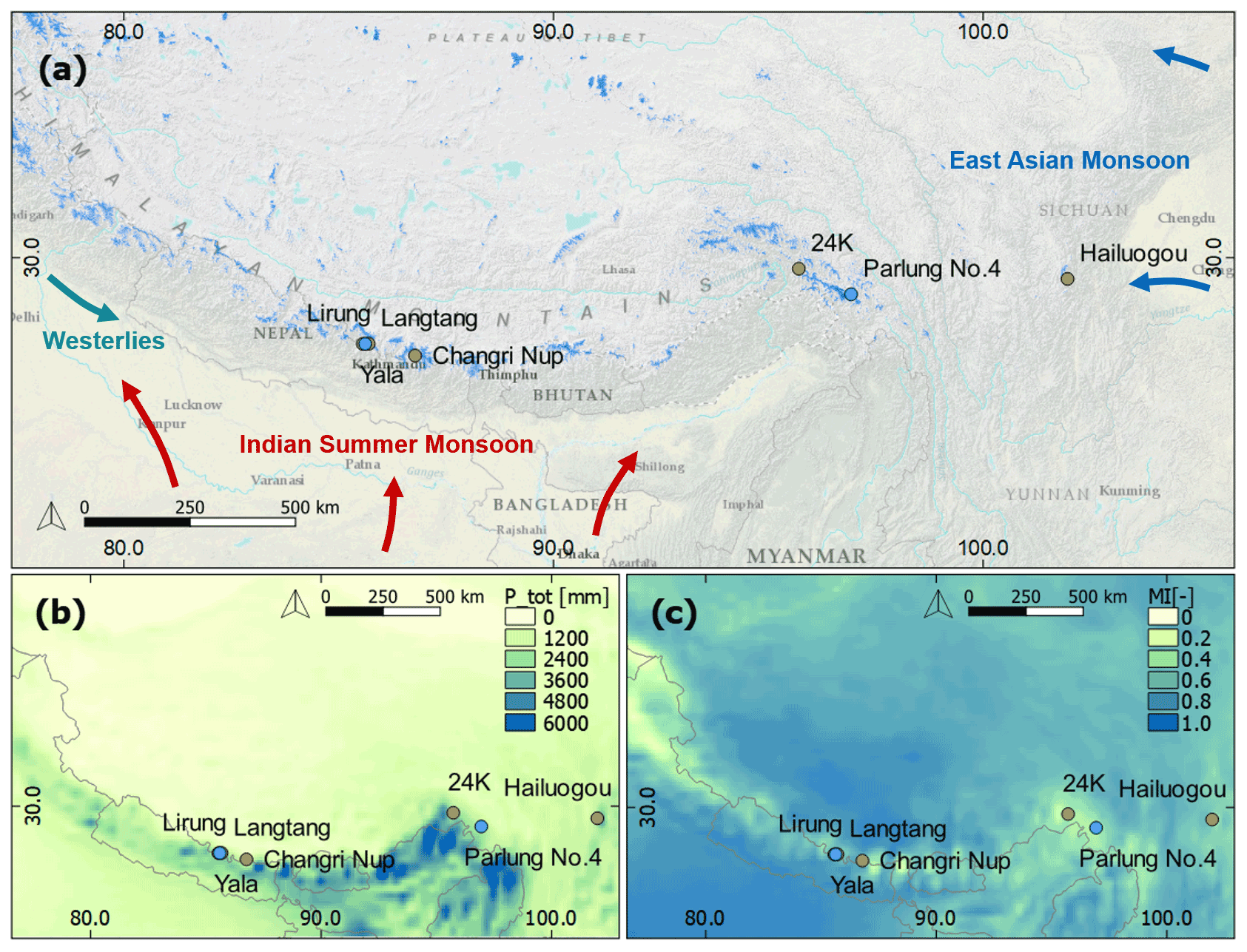
Figure 1(a) The context of study sites with respect to large-scale weather patterns, topography and glacier distribution (blue, source: Randolph Glacier Inventory 6.0). Blue dots indicate clean-ice study glaciers and brown dots indicate debris-covered study glaciers. (b) The spatial pattern of average annual precipitation from ERA5-Land (1981–2019). (c) The monsoonal (June–September) portion of the ERA5-Land total annual precipitation (MI). Background map source: ESRI, U.S. National Park Service.
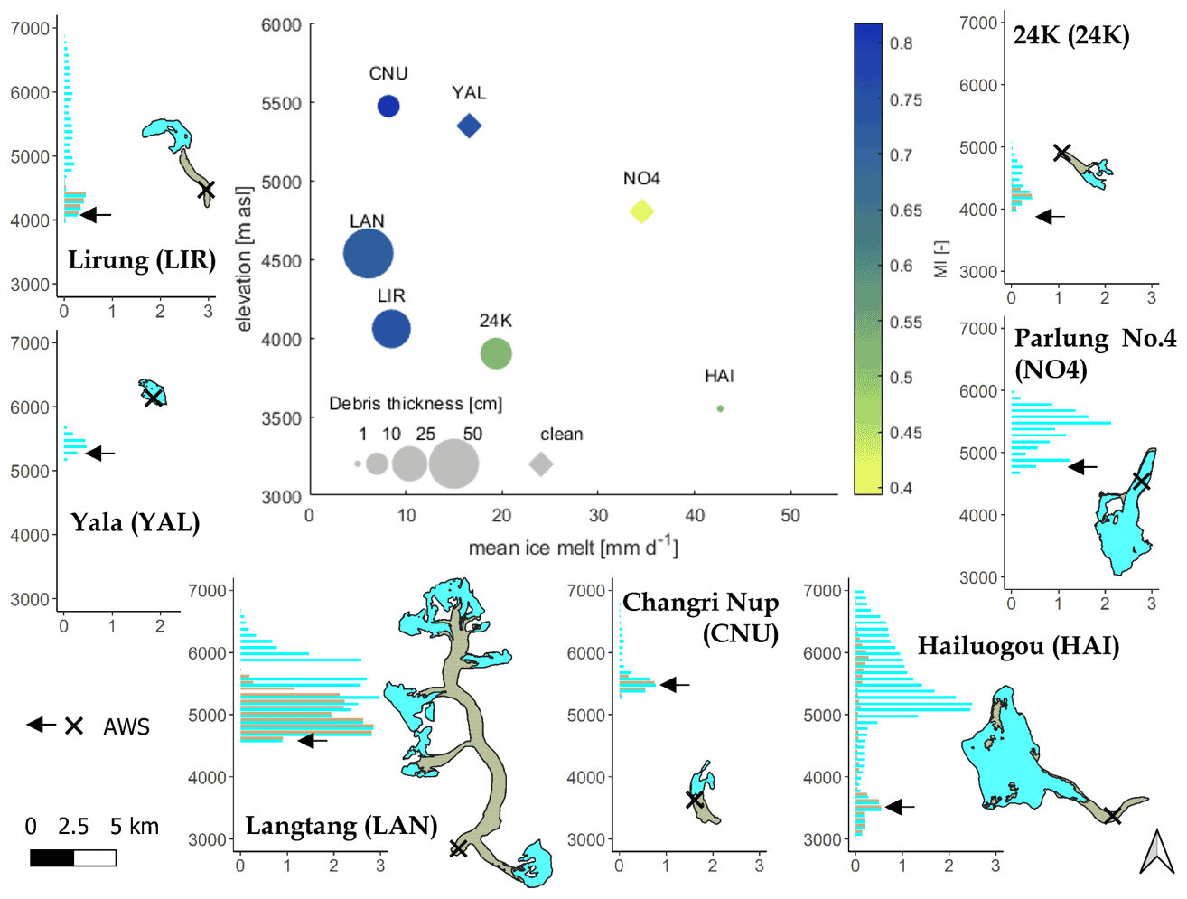
Figure 2Characteristics of study sites, summarised (centre) in terms of elevation, mean measured ice melt rate, measured debris thickness and JJAS contribution to the ERA5-Land total annual (1981–2019) precipitation (monsoon index; MI). For each site, we also show glacier (bars in aqua) and debris (bars in olive) hypsometry, with area on the x-axis [km2] and altitude on the y-axis [m a.s.l.], and glacier and supraglacial debris extents.
Table 1Summary of available meteorological and ablation observations at each site, as well as each site's model period. Variables indicated by * were transferred from neighbouring weather station. Variables with were reconstructed based on other variables measured at the same station.
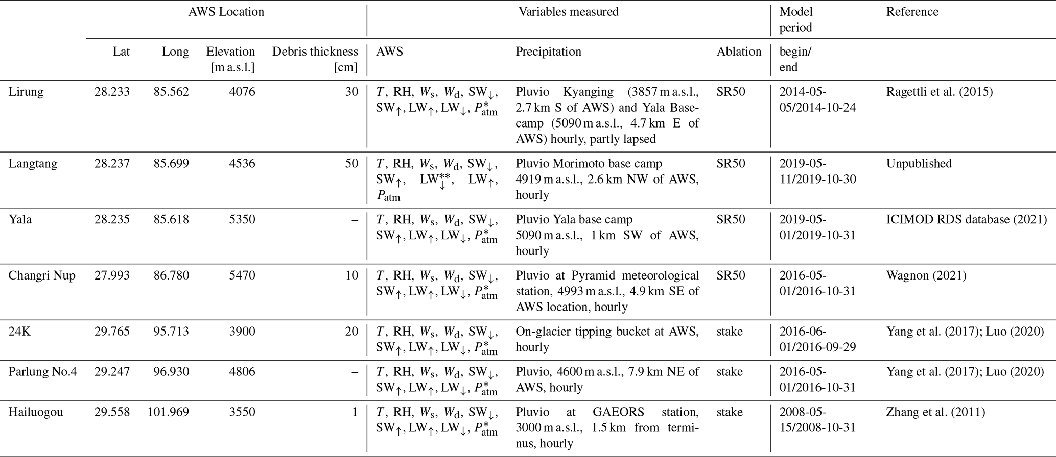
Table 2Characteristics of the study sites. Planimetric glacier and debris surface areas, mean elevation, slope and aspect were calculated using the updated Randolph Glacier Inventory 6.0 by Herreid and Pellicciotti (2020) and the USGS GTOPO30 digital elevation model. Slope (mean) and aspect (vectorial average) for the whole glacier. MI (monsoon index) is the mean June–September portion of the ERA5-Land total annual precipitation (1981–2019); for Lirung, where the ablation zone has dynamically disconnected from the accumulation zone, the glacier characteristics represent both zones together.
3.1 Tethys–Chloris energy-balance model
We use the hydrological, snow and ice modules of the Tethys–Chloris (T&C) land surface model (Fatichi et al., 2012; Paschalis et al., 2018; Mastrotheodoros et al., 2020; Botter et al., 2020) to simulate the mass and energy balance of the seven study glaciers. The T&C model simulates, in a fully distributed manner, the energy and mass budgets of a large range of possible land surfaces, including vegetated land, bare ground, water, snow and ice. Here, we apply the model at the point scale of the AWS locations to simulate the energy fluxes of the underlying surface and subsurface, which can comprise snow, ice and supraglacial debris cover layers, according to the local and dynamic conditions. The melt and accumulation of ice and snow, and the ice melt under debris, are also explicitly simulated. The surface energy balances for the three different possible surfaces are, for snow,
for debris cover,
and for ice,
where Rn [W m−2] is the net radiation absorbed by the snow/debris/ice surface, Qv [W m−2] is the energy advected from precipitation, Qfm [W m−2] is the energy gained or released by melting or refreezing the frozen or liquid water that is held inside the snow pack, H [W m−2] is the sensible energy flux and λE [W m−2] the latent energy flux for any of the surfaces, and G [W m−2] is the conductive energy flux from the surface to the subsurface. In ice, the conduction of energy is represented in the model down to a depth of 2 m after which it is assumed the ice pack is isothermal. Finally, M [W m−2] is the energy available for snow or ice melt. For debris on top of ice, and snow on top of debris or ice, the in-/outgoing fluxes towards/from the ice are adjusted according to the respective interface type. The sign convention is such that fluxes are positive when directed towards the surface. To close the energy balance, a prognostic temperature for the different surface types (Tsno, Tdeb, Tice) is estimated for each computational element. Iterative numerical methods are used to solve the non-linear energy budget equation until convergence for the ice and snow surface, and the heat diffusion equation for the debris surface, while concurrently computing the mass fluxes resulting from snow and ice melt and sublimation. In the case of snow, debris and ice surfaces, either of which is simulated to always fully cover a computational element, Tsno, Tdeb or Tice are equivalent to the element's overall surface temperature Ts. In the following, we use the surface type specific symbol for surface-specific equations, while we use Ts for equations that are valid for all three surface types.
3.1.1 Radiative fluxes
Rn is calculated as the sum of incoming and outgoing shortwave and longwave fluxes as
where SW↓ [W m−2] is the incoming shortwave radiation, α [−] is the surface albedo, LW↓ [W m−2] and LW↑ [W m−2] are the incoming atmospheric and outgoing longwave radiation components, respectively. In this study α is given as an input to the model based on the AWS observations. We prescribe α for all surface types as the daily cumulated albedo, which is the 24 h sum of SW↑ divided by the sum of SW↓ centred over the time of observation (van den Broeke et al., 2004).
3.1.2 Incoming energy with precipitation
For calculating the incoming energy with precipitation, rain is assumed to fall at air temperature (Ta) when positive, with a lower boundary of 0 ∘C. Snow is assumed to fall at negative Ta with an upper boundary of 0 ∘C. Here, Qv is the energy required to equalise the precipitation temperature with the surface temperature Ts and is therefore calculated as:
where cw=4196 [J kg−1 K−1] is the specific heat of water, ci=2093 [J kg−1 K−1] the specific heat of ice, ρw=1000 [kg m−3] is the density of water and Prliq [mm], Prsno [mm] are the rain- and snowfall intensities, respectively.
3.1.3 Phase changes in the snow pack
The snow pack has a water-holding capacity Spwc described in Sect. 3.2.2. The energy flux gained/released by melting/refreezing the frozen/liquid water that is held inside the snow pack is calculated as:
where [–] with is the fraction of the snowpack water equivalent (SWE [mm w.e.]) involved in either melting or freezing. This choice was made in order to mimic refreezing in the upper portion of the snowpack, while the snowpack is otherwise represented as a single layer. λf=333 700 [J kg−1] is the latent energy of melting and freezing of water, t stands for time, dt [s] is the time step, and the unit for Tsno is [∘C].
3.1.4 Turbulent energy fluxes
Over snow, debris and ice surfaces, the sensible energy flux is calculated as:
where Ts [∘C] is the surface temperature (generalised term for Tsno, Tdeb, Tice), [J kg−1 K−1] is the specific heat of air at constant pressure, and ρa [kg m−3] is the density of air. The aerodynamic resistance rah [s m−1] is calculated using the simplified solution of the Monin–Obukhov similarity theory proposed by Mascart et al. (1995) and implemented in Noilhan and Mahfouf (1996); for details see also Supplement Sect. S3. The roughness lengths of heat (z0h [m]) and water vapour (z0w [m]) used in the calculation of the aerodynamic resistance are equal in the T&C model (z0h=z0w), and (), with further details on these choices provided in the Supplement Sect. S3. The roughness length of momentum (z0m) is set to 0.001 m for snow and ice surfaces (Brock et al., 2000), while we optimise it against the surface temperature for debris (see Sect. 3.3).
Correct estimates of the latent energy flux due to water phase changes at the surface are important for accurately modelling glacier melt, especially under moist conditions (Sakai et al., 2004). Phase changes between the water and gas phase and the resulting energy fluxes are considered over all surfaces. The latent energy is limited by the availability of water in the form of ice and snow, or in the case of a debris surface, by the amount of water intercepted (interception storage capacity is set to 2 mm). The latent energy flux is estimated from:
where λs is the latent energy of sublimation defined as , with [J kg−1] as the latent energy of vaporisation. qsat is the surface specific humidity at saturation at Ts, qa is the specific humidity of air at the measurement height and raw the aerodynamic resistance to the vapour flux, which we assume equals rah.
3.1.5 Ground energy flux
The definition of the ground energy flux G [W m−2] differs based on the surface type. When there is snow, it is equal to the energy transferred from the snowpack to the underlying ice or debris surface. The snow pack is represented as a single layer. In the assumption of a slowly changing process, G can be approximated with the temperature difference of the previous time step (t−1), which allows us to solve for G outside the numerical iteration to find the snow surface temperature of the current time step:
where ksno [W K−1 m−1] is the thermal conductivity of snow and dsno [m] is the snow depth. For ice, in the absence of snow and debris, it is the energy flux from the ice pack to the underlying surface or to the ice at a depth of 2 m:
where kice [W K−1 m−1] is the thermal conductivity of ice, Tgrd [∘C] is the temperature of the underlying ice, and dice [m] is the relevant ice thickness. The ice pack was not discretised into sub-layers. For debris, which was discretised into eight layers at all debris-covered sites, G is the energy flux conducted into the debris layers. Its calculation for a given time t and depth z is
where kd [W K−1 m−1] is the debris thermal conductivity (see Sect. 3.3) and Tdeb(z,t) [∘C] is the debris temperature at time t and depth z. G(z,t) can be included in the heat diffusion equation as such:
where cvd is the debris heat capacity. Under the assumption of homogeneous debris layers, κ [m2 s−1] as the debris heat diffusivity replaces the term and Eq. (12) can be written as:
The heat diffusion equation (Eq. 13) is solved using iterative numerical methods. This way, the debris temperature profile Tdeb(z,t) is solved together with G(z,t) at any depth and time. The conductive energy flux at the base of the debris is used to heat the ice and to calculate ice melt once above the melting point.
Note, that G can also act in the opposite direction, i.e. when energy is conducted from the snow pack/debris/ice towards the surface. In our results, G sums up all types of conductive energy fluxes in the snow–debris–ice column.
3.2 Mass balance in the T&C model
3.2.1 Precipitation partition
Precipitation is partitioned into solid Prsno and liquid Prliq precipitation, because of the differing impacts of snow and rain on the energy and mass balance. For this study, the precipitation partition method described by Ding et al. (2014) was implemented into the T&C model. This parameterisation has been developed specifically for High Mountain Asia based on a large dataset of rain, sleet and snow observations, and does not require recalibration. It determines the precipitation partition based on the wet-bulb temperature, station elevation and relative humidity and allows for sleet events, as a mixture between liquid and solid precipitation. Ding et al. (2014) found the wet-bulb (Twb) to be a better predictor than Ta of the precipitation type. They also found that the temperature threshold between snow and rain increases at higher elevations, and that the probability of sleet is reduced in conditions of low relative humidity.
3.2.2 Water content of the snow, ice and debris layers
The water content of ice is approximated with a linear reservoir model. The liquid water outflow is proportional to the ice pack water content Ipwc [mm w.e.], which is initiated when Ipwc exceeds a threshold capacity, prescribed as 1 % of the ice water equivalent (IWE [mm w.e.]). The Ipwc is the sum of ice melt and liquid precipitation, minus the water released from the ice pack. The water released is the sum of the ice pack excess water content plus the outflow from the linear reservoir, given as , where Kice is the reservoir constant which is proportional to the ice pack water equivalent. Unlike within snow packs, Qfm is not accounted for within the ice pack, since water is presumed to be evacuated quickly from the ice due to runoff without refreezing.
The water content of the snow pack Spwc [mm w.e.] is approximated using a bucket model, in which outflow of water from the snow pack occurs when the maximum holding capacity of the snow pack is exceeded. Following the method of Bélair et al. (2003), the maximum holding capacity of the snow pack is based on SWE, a holding capacity coefficient and the density of snow ρsno. Snowmelt plus liquid precipitation, minus the water released from the snow pack gives the current Spwc. If Tsno is greater than 0 ∘C then the snow pack water content is assumed to be liquid, whereas otherwise it is assumed to be frozen.
For supraglacial debris, both observations and methods for modelling its water content are lacking. We thus use a simplified scheme for moisture at the surface of the debris, in order to mimic the drying process of the debris surface: We assume debris to have a dynamic interception storage sIn, which can hold a maximum of mm water at all debris-covered sites and can be refilled by snowmelt or liquid precipitation. The evaporative flux from the debris is limited by the state of this interception storage and LE can only result from evaporation if sIn>0. The term In [%] (used in Sect. 4.5 and Fig. 9b) is the percentage of time during which this condition is met.
3.2.3 Snow and ice mass balance
The mass-balance calculation of snow and ice is somewhat similar, and therefore they are described together here. Calculations are performed for snow if there is snow precipitation during a time step or the modelled SWE at the surface is greater than zero. Net input of energy to the snow or ice pack will increase its temperature, and after the temperature has been raised to the melting point, additional energy inputs will result in melt. The change in the average temperature of the ice or snowpack dT is controlled using
where dt is the time step [h] and WEb [mm w.e.] is IWE or SWE before melting and limited to a maximum of 2000 mm, assumed to be the water equivalent mass exchanging energy with the surface. Energy inputs into an iso-thermal ice/snow pack result in melt m [mm w.e.] as
The water equivalent mass of the snow/ice pack after melting WE(t) [mm w.e.] is updated conserving the mass balance following:
Here [mm] is the sublimation from ice and snow. The snow density is assumed to be constant with depth, and calculations are performed assuming one single snow pack layer. The snow density evolves over time using the method proposed by Verseghy (1991) and improved by Bélair et al. (2003). In this parameterisation the snow density increases exponentially over time due to gravitational settling and is updated when fresh snow is added to the snowpack. Two parameters are required in this scheme, and [kg m−3], which represent the maximum snow density under melting and freezing conditions, respectively. The depth of the ice pack can be increased through the formation of ice from the snow pack (ice accumulation), which is prescribed to occur if the snow density increases to greater than 500 kg m−3 (a density associated with the firn-to-ice transition) and at a rate of 0.037 mm h−1 (Cuffey and Paterson, 2010). The density of ice is assumed constant with depth and equal to 916.2 kg m−3.
3.3 Debris parameters
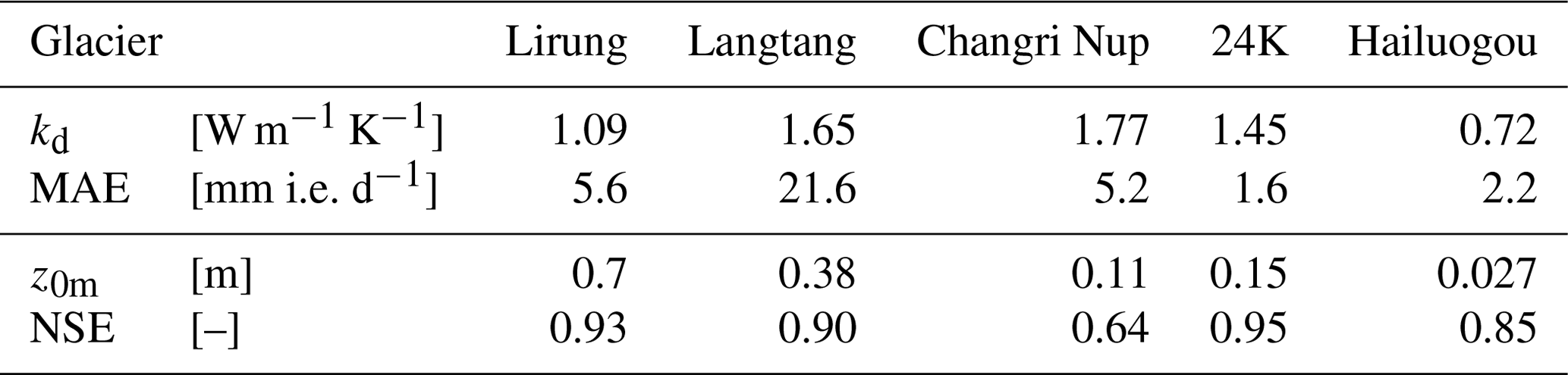
A major challenge in physically based mass-balance modelling of debris-covered glaciers is the selection of appropriate debris properties. In addition to the debris thickness, which was measured at the AWS location, values are needed for the thermal conductivity kd, the aerodynamic roughness lengths z0m, z0h and z0w of the debris surface, the surface emissivity ϵd, the debris volumetric heat capacity cvd and the debris density ρd. While the last three can be quantified using values from the literature, there is more uncertainty about kd and the roughness lengths, which are highly variable quantities that are difficult to measure in the field. We thus choose to optimise them, since our primary requirement is an accurate representation of the energy and mass balance: (1) in a first step, we optimise kd simulating only the conduction of energy through the debris during snow-free conditions, with the LW↑-derived surface temperature Ts,LW as an input, the ice melt as the target variable and the Nash–Sutcliffe Efficiency (NSE [–]) as performance metric. (2) Next, we run the whole energy-balance model and optimise z0m, and with it z0h and z0w, which are linked to z0m via a fixed ratio (for details, see Sect. S3). We use the AWS records for snow-free conditions, with all required meteorological inputs, and the optimal kd from step (1), while comparing modelled Ts against Ts,LW, using NSE as performance metric. The resulting parameters are given in Table 3. All optimised values fall within the expected range based on prior energy-balance studies of debris-covered glaciers (Nicholson and Benn, 2006; Reid and Brock, 2010; Lejeune et al., 2013; Rounce et al., 2015; Collier et al., 2015; Evatt et al., 2015; Yang et al., 2017; Miles et al., 2017; Quincey et al., 2017; McCarthy, 2018; Rowan et al., 2020).
Table 3Optimum debris parameters kd and mean absolute error (MAE) from optimisation step 1 (modelled vs measured melt); z0m and Nash–Sutcliffe Efficiency (NSE) from optimisation step 2 (modelled vs measured surface temperature).
3.4 Uncertainty estimation
We calculate the uncertainty associated with all energy- and mass-balance components by performing 103 Monte Carlo simulations for each study site at the AWS location. We perturb three debris parameters (kd, z0m, ϵd), debris thickness hd, as well as six measured model input variables: air temperature Ta, the vapour pressure at reference height ea [Pa], SW↑, SW↓, LW↓, the total precipitation before partition Pr, and the wind speed Ws. Measured outgoing shortwave radiation SW↑ was included into the Monte Carlo set, as it determines our input α, as discussed in Sect. 3.1.1. While the parameter uncertainty range was defined based on previously published values for debris (e.g. Yang et al., 2017; Rounce et al., 2015; Evatt et al., 2015; Reid and Brock, 2010; Nicholson and Benn, 2006; Rowan et al., 2020; Lejeune et al., 2013; Collier et al., 2015; Miles et al., 2017; Quincey et al., 2017; McCarthy, 2018), the debris thickness measurement uncertainty was given with a range of 1 cm and the range for the meteorological inputs was set based on the respective sensor uncertainties (see Table 4). All uncertainties were equally distributed around the standard parameter values and observations. Uncertainties are given as one standard deviation of the error of the Monte Carlo runs against the standard run.
Table 4Uncertainty ranges of parameters and input variables used for Monte Carlo runs. Where units are indicated with [–], the parameter or variable was perturbed by the fractional value shown.
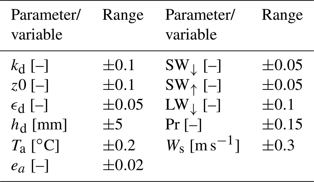
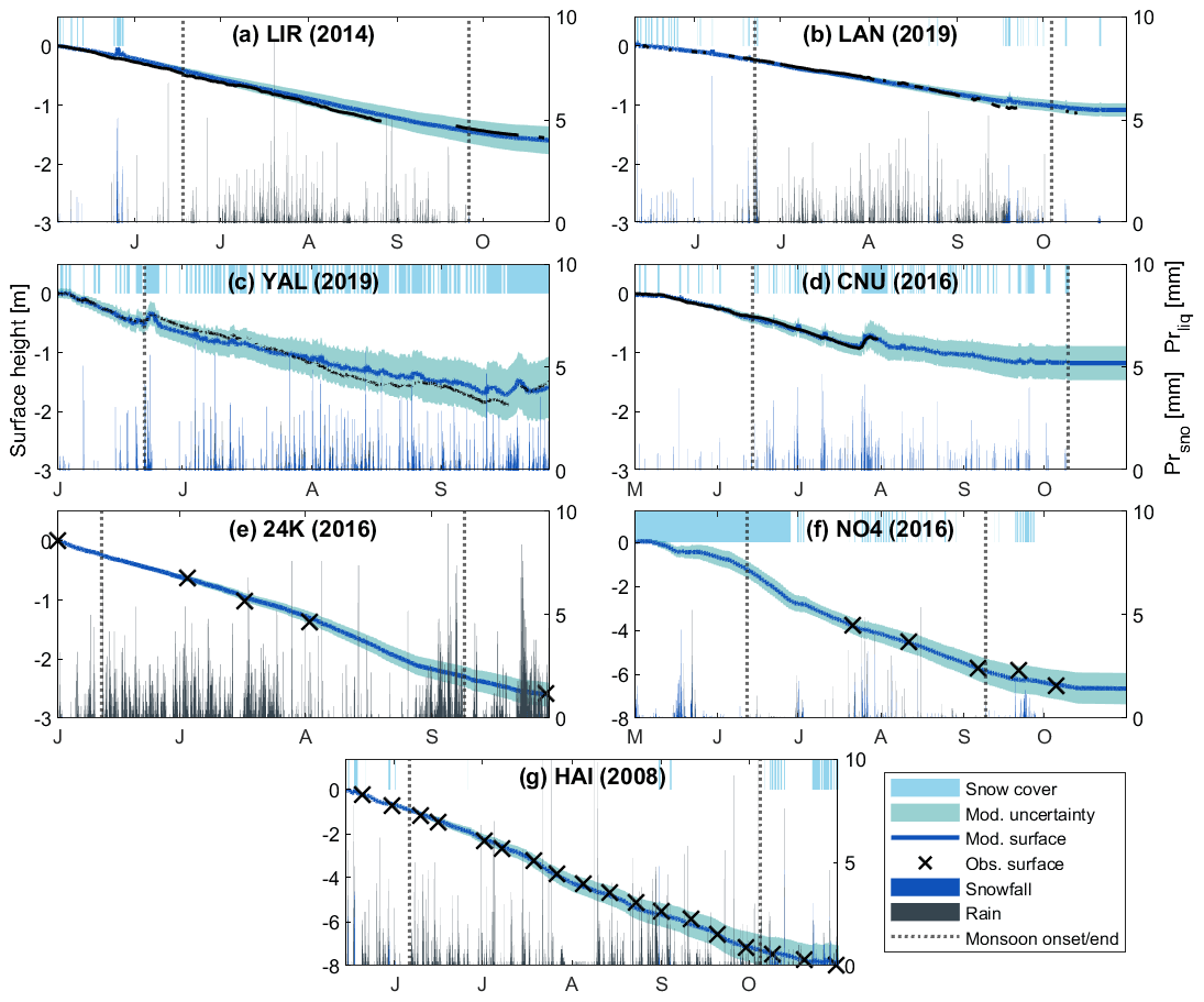
Figure 3(a–g) Observed vs modelled surface change at all study sites, precipitation phase and snow cover timing. Measured melt is either from ablation stakes (black crosses) or ultrasonic depth gauges (black lines). Vertical dotted lines indicate monsoon onset and end.
3.5 Model evaluation
The model accurately reproduces the measured surface height change (ablation and accumulation) at both debris-covered and clean-ice glaciers (Fig. 3). The maximum uncertainties associated with each model output ranges from ±11 % (Parlung No.4, Fig. 3f) to ±33 % (Yala, Fig. 3c). Where ultrasonic depth gauge (UDG) records are available (Lirung, Langtang, Yala, Changri Nup), the deviations of the simulations from the observations remain within the uncertainty range (Fig. 3a–d). We decided to not consider the UDG record from Changri Nup after a large August snowfall, as variables describing the surface state (e.g. α, LW↑) following this event indicate a discontinuous snow cover at the AWS location, while the UDG, which is some metres away from the AWS, shows continuous snow cover with depths of tens of centimetres. This discrepancy was also confirmed by observation of the site from October 2016. It was thus not possible to match the UDG record with the model for the late ablation period on Changri Nup, but the model closely reproduces observed surface height change for the pre-monsoon and early monsoon (Fig. 3d), when AWS and UDG observations agree in terms of surface state. The deviation to measured melt stays within the uncertainty range at 24K, Parlung No.4 and Hailuogou (Fig. 3e, f). For Parlung No.4 there are no stake measurements available before 21 July due to the long-lasting snow cover.
4.1 Modelled mass balance
The ablation season average melt rates vary considerably across sites: The highest value of 42.7 mm d−1 is reached at the low-lying site with thin debris cover, Hailuogou, and the lowest value of 6.1 mm d−1 is evident at Langtang, a site at moderate elevation but with the thickest debris cover out of all study sites (Fig. 4). The largest average seasonal mass loss component at all sites is ice melt, with a minimum of 65.8 % of the mass losses at Changri Nup (Fig. 4c) and up to 95.4 % at Hailuogou, (Fig. 4g). This is followed by snowmelt, accounting for only 0.1 % at 24K (Fig. 4e) but as much as 33.1 % at Yala (Fig. 4c) of the seasonal mass losses. Sublimation from ice and snow represents a very small share of the seasonal mass losses, and ranges from 0.01 % (Lirung, Fig. 4a) to 1.2 % (Changri Nup, Fig. 4d). It mostly occurs under dry conditions during pre-monsoon at the highest sites (Changri Nup, Yala).
The timing of snow cover is an important control both of the amounts and of the patterns of ice melt, as ice melt rates are close to zero during periods of snow cover. This becomes clear in Fig. 4, where ice melt rates are low during weeks when also snowmelt takes place. A long-lasting pre-monsoonal snowpack can delay the onset of ice melt considerably, e.g. at Parlung No.4, where ice melt is delayed until the end of June (Figs. 3f and 4f). Similarly, intermittent snow cover protects the ice from melting at the two highest sites (Yala and Changri Nup) during the summer months (Figs. 3c–d and 4c–d).
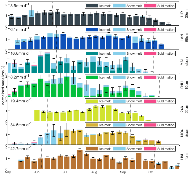
Figure 4Melt rates of ice and snow (stacked) as weekly averages at each site. Vertical dotted lines indicate monsoon onset and end. Error bars depict the uncertainty (standard deviation) of the estimates. Melt rates are normalised to the mean of the ice melt over the entire period (value in the upper left of each panel).
4.2 Modelled energy balance
The largest components in the energy balance are LW↑, LW↓ and SW↓ (Fig. S9). The two longwave fluxes counteract and offset each other in large parts resulting in a moderate, melt-reducing LWnet, which reaches its highest values during the pre- and post-monsoon periods (Fig. 5). SW↓ and its reflected counterpart SW↑ result in a net shortwave flux SWnet, which at all sites contributes the overall largest amount of energy available for melt M (Fig. 5). M is additionally increased or reduced by the turbulent fluxes H and LE, while the energy advected to the glacier surface by precipitation (Qv) remains small (<2 W m−2, Table S3). G links the snow/debris/ice surface to the subsurface, and is a result of all surface fluxes and the subsurface conditions. Before ice melt occurs, depending on the season and site, a part dG of G between 0 and 17.8 W m−2 is invested into warming the debris or ice pack to the melting point (Table S3). dG tends to be larger during pre-monsoon and at the higher sites (Yala, Changri Nup), where air temperatures frequently fall below 0 ∘C.

Figure 5(a–g) Stacked energy fluxes weekly averages at each site, depicting the components SWnet, LWnet, H, LE, Qv, Qfm, G and M. Energy fluxes are negative fluxes when directed away from the surface and positive when directed towards the surface.
4.3 Impact of debris cover
Debris cover modulates the energy balance in several ways: With the albedo of the snow-free debris surface ranging between 0.05 (24K) and 0.22 (Changri Nup), a much larger amount of SW↓ is absorbed by the surface than on clean ice glaciers, where the albedo typically ranges between 0.3 and 0.6. In contrast to clean-ice glaciers, however, where the main flux re-emitting absorbed energy is LW↑ (Fig. 5c and f), a large part of the debris-absorbed energy is also returned to the atmosphere by the turbulent fluxes H and LE (Fig. 5a, b, d and e). As a result of this insulating effect of debris, the seasonal average melt rate of debris-covered 24K is considerably lower (19.4 mm d−1) than that of clean-ice Parlung No.4 (34.6 mm d−1), despite the latter site being 900 m lower in elevation than the former (Fig. 4e and f), and despite their geographical proximity (Fig. 1). On Hailuogou, the site with very thin debris, however, the turbulent fluxes act in the opposite direction, i.e. contributing energy for melt. Summed up, they can reach weekly averages of 150 W m−2 (Fig. 5g).
4.4 Impact of the monsoon
During monsoonal conditions, increased cloudiness results in SW↓ decreasing its melt contribution at all sites compared to pre-monsoonal conditions (Fig. 6) with changes ranging between −41.8 (Hailuogou, pre-monsoon: 178.2; monsoon: 136.4) and −135 (Yala, pre-monsoon: 307.7; monsoon: 172.7) at the seven sites (all values in W m−2, from Table S3). Note that we express fluxes in terms of the net energy absorbed by, or removed from, the snow/debris/ice surface (with positive and negative fluxes indicating energy absorbed and removed from the surface, respectively). Reflected shortwave radiation SW↑, which removes energy from the surface, and which is controlled by the surface albedo, becomes less negative (Fig. 6), by +5.4 (24K, pre-monsoon: −18.5, monsoon: −13.8) and up to +164.8 (Parlung No.4, pre-monsoon: −219.6, monsoon: −54.8) between sites. An exception to this is Changri Nup, where SW↑ becomes more negative by −12.1 W m−2 (pre-monsoon: −60.6, monsoon: −72.7), as a consequence of the high albedo of ephemeral monsoonal snow cover (Fig. 3e, Table S3). On the other hand, the melt contribution of LW↓ increases at all sites (Fig. 6), by at least +15.7 (Hailuogou, pre-monsoon: 314.6, monsoon: 330.3) and up to +57.0 (Yala, pre-monsoon: 248.5, monsoon: 305.5) (Table S3). Its counterpart LW↑ further reduces melt, but to a lesser extent, by −1.0 (Changri Nup, pre-monsoon: −318.7, monsoon: −319.7) to −13.5 W m−2 (Langtang, pre-monsoon: −339.3, monsoon: −352.8) (Table S3). This balancing of the two LW components changes LWnet in the same direction at all sites over the diurnal cycle, with greater changes during the sunlit hours and smaller changes during the dawning and night-time hours (Fig. 7). As a result, LWnet plays only a minor role in cooling the glaciers at all sites during monsoon (Fig. 5).
4.4.1 Impact of the monsoon on clean-ice sites
We observe opposite changes in M at the two clean-ice glaciers in the transition from pre-monsoon to monsoon: M becomes less negative (implying less melt) at Yala by +10.2 (pre-monsoon: −74.8, monsoon: −64.6) and more negative at Parlung No.4 (implying more melt) by −130.4 (pre-monsoon:−32.3, monsoon: −162.6) (all values in W m−2, from Table S3). The difference in M is largely caused by the variability in SWnet, which almost entirely controls the melt of the clean-ice glaciers during monsoon. On Parlung No.4 the SWnet changes are dominated by variations in SW↑, whereas on Yala, SW↓ dominates. Hence, the bulk of changes in the diurnal melt cycle happen during the sunlit hours (Fig. 7b, d). Both H and LE remain comparably small energy fluxes at the clean-ice sites with highest averages of at Parlung No.4 and of at Yala during the pre-monsoon period (Table S3). At Parlung No.4, as much as 12.3 is added to the surface in the form of H during monsoon. Interestingly, LE changes from being a melt-reducing energy flux, emerging from sublimation during pre-monsoon, to a small melt-contributing energy flux from condensation (< 4) at both clean-ice sites (Table S3).
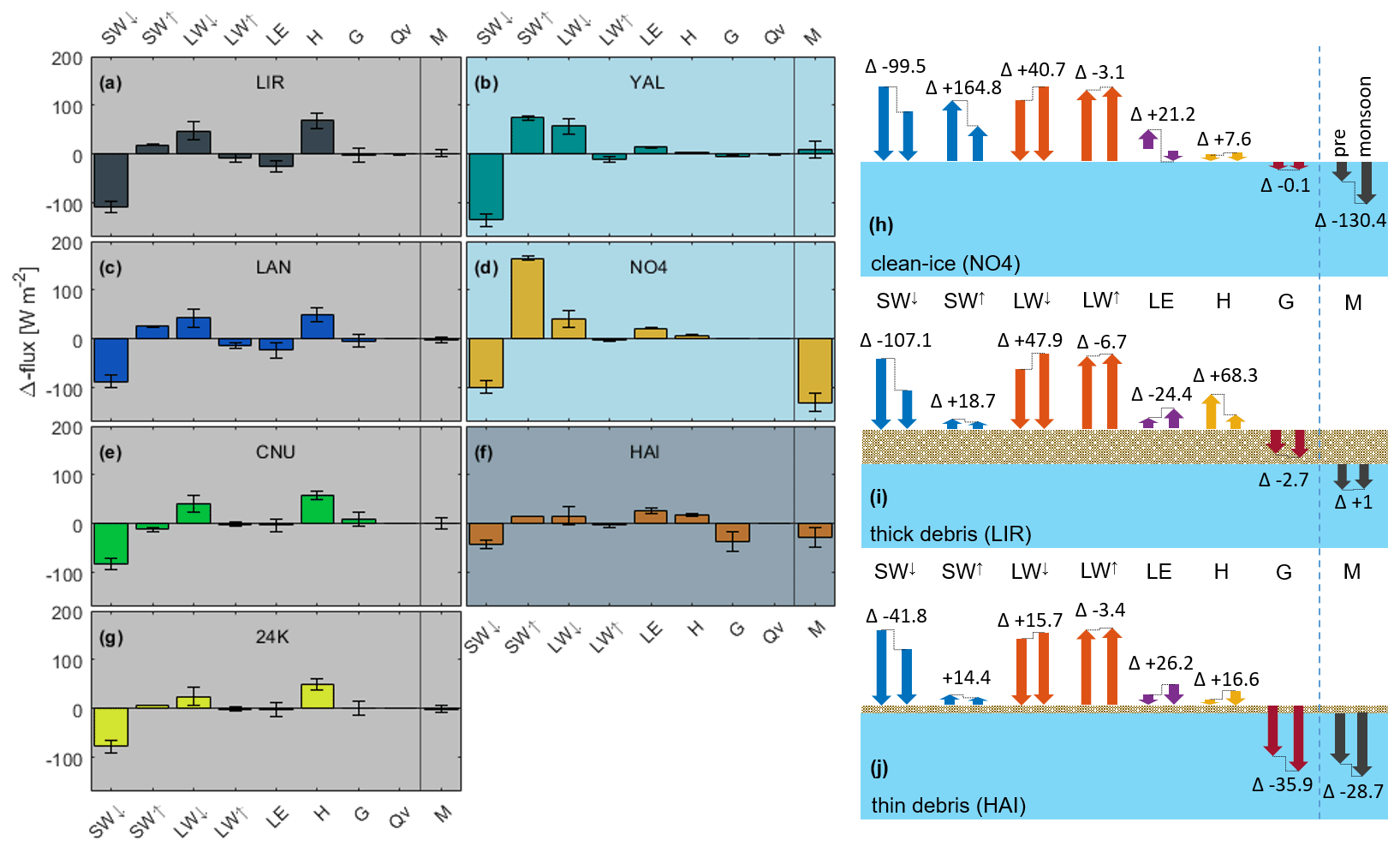
Figure 6(a–g) Differences in energy-balance components from pre-monsoon to monsoon at each site including their uncertainties (error bars). The direction of change is to be considered relative to the sign of the original flux (x-axis). Due to the sign convention mentioned in Sect. 4.3, the changes presented here reflect whether the surface receives more energy (positive change) or less energy (negative change). Background indicates the surface type of the site: grey indicates thick debris cover, light blue indicates clean-ice sites, and grey-blue indicates thin debris. (h–j) Alternative depiction of the changes from (a)–(f), summarising surface types. Example Δ-flux numbers in [W m−2] refer to (h) Parlung No.4, (i) Lirung and (j) Hailuogou; numbers for the remaining glaciers can be looked up in Table S3.
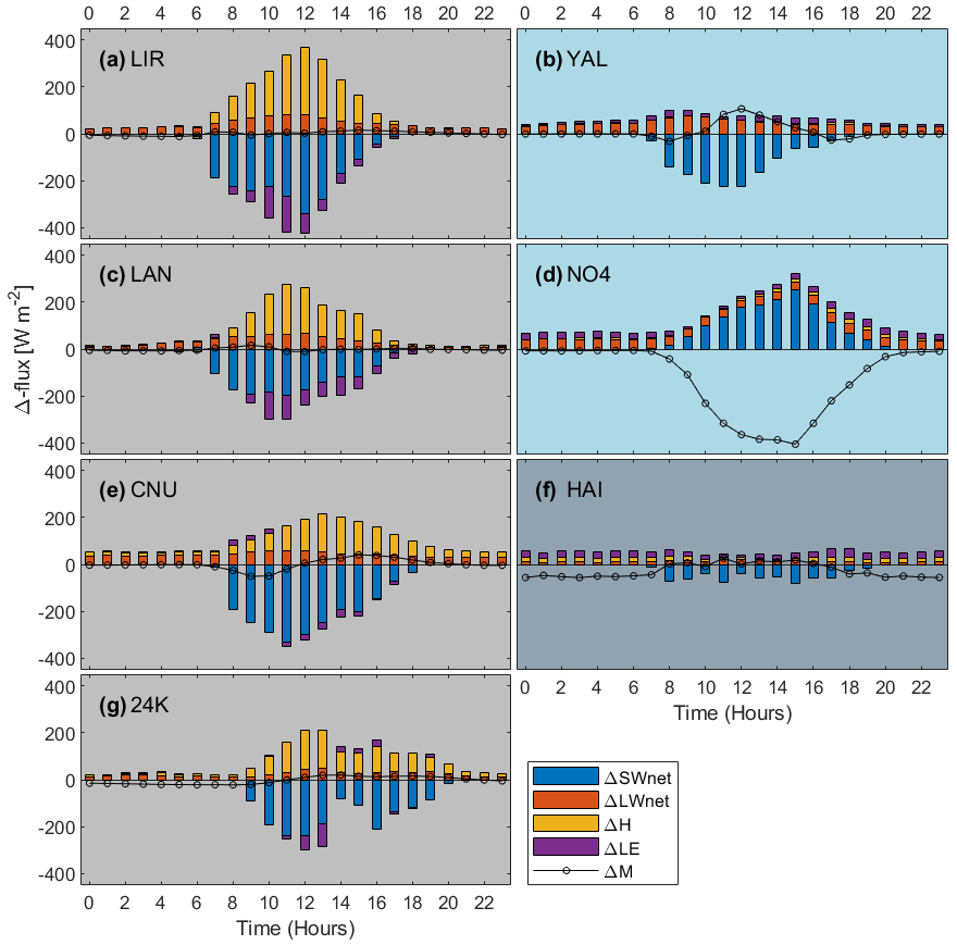
Figure 7Energy flux differences in the diurnal cycle (stacked) between pre-monsoon and monsoon. The direction of change is to be considered relative to the sign of the original flux. Positive and negative sign corresponds to energy added or removed from the glacier, respectively; grey background indicates debris-covered site, light blue indicates clean-ice sites and grey-blue indicates 1 cm debris site
4.4.2 Impact of the monsoon on glaciers with thick debris
Average M remains similar between pre-monsoon and monsoon at the sites with thick debris cover, as the energy-balance components adjust to monsoonal conditions: the changes in M, ranging between +1.0 (Lirung, pre-monsoon: −37.5, monsoon: −36.5) and −2.1 (24K, pre-monsoon: −79.5, monsoon: −81.6), stay below uncertainty levels (all values in W m−2, Fig. 6a, c, e, g and Table S3). Similar to the other surface types, LWnet reduces melt to a lesser degree during the monsoon period (Sect. 4.4). There is a considerable reduction in the melt contribution of SWnet, and the glacier-cooling H becomes less negative by 49.0 (24K, pre-monsoon: −99.8, monsoon: −50.8) up to 68.3 (Lirung, pre-monsoon: −116.7, monsoon: −48.4) (Table S3). The change in LE partly offsets the changes in H, with LE becoming more negative, from −2.1 (24K, pre-monsoon: −50.6, monsoon: −52.7) to −24.4 (Lirung, pre-monsoon: −16.0, monsoon: −40.4) (Fig. 6a, c, e and g, and Table S3). Therefore, the changes in the average fluxes from pre-monsoon to monsoon tend to balance each other out (reduced SW↓ and more negative LE are balanced by increased LW↓ and less negative H), so that overall melt rates remain similar. This balancing is also visible in the diurnal cycle of changes at Lirung, Changri Nup and 24K, where there is an increase in M during the night-time and morning hours, but a decrease in the afternoon hours (Fig. 7a, e, g). At Changri Nup (Fig. 7e), the pattern is accompanied by a lag of around 4 h between the peak changes of the radiative and turbulent fluxes.
An interruption of the monsoon at 24K occurred in August 2016, possibly associated with an El Niño event (Kumar et al., 2006). During this interruption the energy balance returned to a pre-monsoonal regime (Fig. 5e) due to clearer skies, more pronounced diurnal temperature amplitudes, low precipitation rates and lower relative humidity (Fig. S6). This left a clear imprint in the diurnal cycle of changes (absence of heavy afternoon overcast in comparison with the other sites, Fig. 7g) and resulted in higher melt rates during that period (Fig. 4e).
4.4.3 Impact of the monsoon on a glacier with thin debris
In contrast to the glaciers with thick debris, during the monsoon, M becomes considerably more negative (more melt) at Hailuogou Glacier. Although SWnet contributes less energy for melt during the monsoon and LWnet remains overall small at this site (Fig. 5), M became more negative by −28.7 (pre-monsoon: −158.1, monsoon: −186.8) on average (all values in W m−2, from Table S3), and mostly during the nights (Fig. 7f). The increase in melt energy is mostly driven by the turbulent energy fluxes: H increases by 16.6 (pre-monsoon: 9.1, monsoon: 25.7) and LE increases by 26.6 (pre-monsoon: 5.4 monsoon: 31.6) (Fig. 5 and Table S3), with higher increases during the night-time than during the daytime (Fig. 7f). While they act to reduce melt at the glaciers with thick debris cover, here the turbulent fluxes drive additional melt during the monsoon.
4.4.4 Sensitivity of seasonal flux changes to elevation and debris thickness
Our results are derived from simulations at one location (AWS) on each glacier. To understand how representative our results are of conditions across the glacier ablation zone at each site, and across the possible range of debris thicknesses in particular (Table S4), we conduct a sensitivity experiment to evaluate the transferability of our results across the glaciers' ablation areas (see detailed explanation in Supplement Sect. S5). This experiment shows that even accounting for the range of conditions across each glacier ablation area, the pattern of pre-monsoon to monsoon difference in flux components, and importantly the equalising effect on M, remains similar at the glacier scale at all sites with thick debris cover (Fig. 8).

Figure 8Changes in the individual fluxes when moving from pre-monsoon to monsoon. Colour dots indicate `standard' runs with AWS site-specific conditions. Black bars indicate the uncertainty range on the standard runs. Grey indicates the sensitivity of flux changes (Δ-range) to elevation and debris thickness (debris-covered glaciers only). Ranges of elevation and debris thicknesses used here are given in Table S4. Positive and negative sign corresponds to energy added or removed from the glacier, respectively.
4.5 Controls on the turbulent fluxes
Our results show the importance of the turbulent fluxes in the energy balance of debris-covered glaciers, their varying role as melt-enhancing or melt-reducing fluxes depending on the debris thickness, and how the monsoon modulates them.
To assess the controls on the turbulent fluxes, we regressed the modelled values of H and LE against climatic variables (see Supplement Sect. S6). We find that H is largely controlled by the temperature gradient between surface and air (δT) on glaciers with thick debris: between 72 (Lirung, pre-monsoon) and 97 % (24K, pre-monsoon) of the variability of H is explained by δT (Fig. 9a), and δT decreases during monsoonal conditions by −0.05 (Langtang) to −1.44 ∘C m−1 (Changri Nup) (Table S1). It becomes clear that a smaller temperature gradient between surface and air during the monsoon weakens the melt-reducing effect of H. By contrast, Ws emerges as the most important control of H and LE at the glacier with thin debris, explaining up to 91 % and 65 % of the variability, respectively (Fig. 9a). The mean magnitude of Ws increases at this site from 1.23 in pre-monsoon to 2.15 m s−1 in monsoon (Table S1). A cold surface in combination with a wind-enhanced turbulence and fast turnover of warm and moist air masses results in both H and LE becoming powerful drivers of melt on Hailuogou, the glacier with thin debris cover (Fig. 5).
Across the sites with thick debris, vpd has somewhat more power than Ws in explaining LE (Fig. 9a), but combined, their explanatory power does not exceed 52 % (Lirung). An exception is the pre-monsoon at Changri Nup, where the combination of vpd and Ws explains 71 % of the variability. Yet, LE increases consistently from pre-monsoon to monsoon together with an increase in the duration of moisture availability at the surface of those glaciers, with increases ranging between 22.3 % at 24k and 63.1 % at Changri Nup (Table S1). In fact, evaporation and its melt-reducing LE flux tend to be water-limited during the pre-monsoon, but energy-limited during the monsoon (Fig. 9b). This implies that the availability of additional moisture drives the increase of LE from pre-monsoon to monsoon.
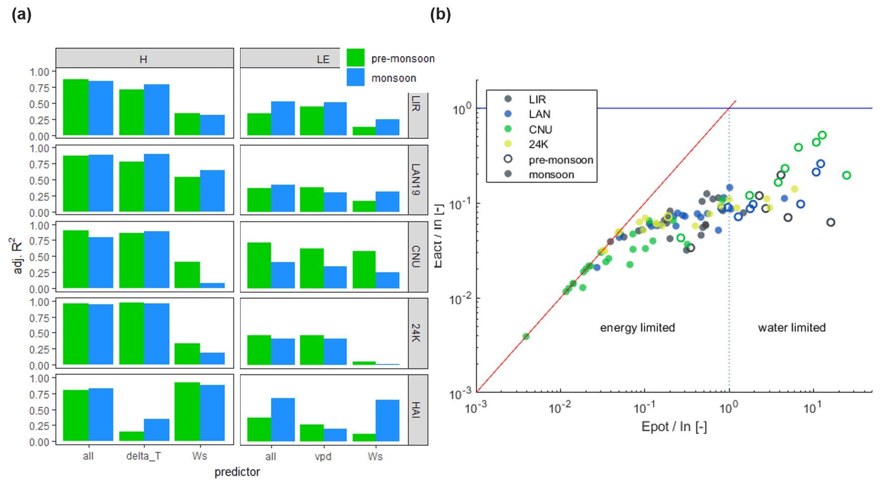
Figure 9(a) Left: Predictive power of temperature gradient between surface and air (δT) and wind speed (Ws) and their combination (`all') for determining H. (a) Right: Predictive power of temperature gradient between surface and air (vpd) and wind speed (Ws) and their combination (`all') for determining LE. Details on the predictors and regression models used are given in Sect. S6. (b) Budyko-like diagram with the 5 d mean potential evaporation rate during snow-free conditions (Epot) relative to the mean available intercepted water (In) on the x-axis, and the actual evaporation rate during snow-free conditions (Eact) relative to In on the y-axis. Only debris-covered glaciers where LE is a glacier-cooling flux are shown.
5.1 Which mass and energy fluxes determine the seasonal mass balance of glaciers in the Central and Eastern Himalaya?
We apply our model in a systematic way to seven glaciers in a variety of environments in the Central and Eastern Himalaya. We force the model with in situ station data and constrain and evaluate it against observations of surface height change, lending great confidence to the energy flux components. Previous energy-balance studies in the region were limited to two (Lejeune et al., 2013; Yang et al., 2017; Bonekamp et al., 2019) or three (Zhu et al., 2018) study sites, and partly relied on re-analysis products or atmospheric modelling for forcing (Zhu et al., 2018; Bonekamp et al., 2019), without the possibility to evaluate the model performance. At all our study sites, ice melt is the largest mass loss component during the ablation season, followed by snowmelt, while sublimation plays only a small role early and late in the season (Sect. 4.1). Similar to several previous studies (Kayastha et al., 1999; Aizen et al., 2002; Yang et al., 2011; Sun et al., 2014), we find that the largest energy source for snow and ice melt is SWnet (Sect. 4.2). Thus, major controls on the energy and mass balance of all glaciers are the snow cover dynamics (Zhu et al., 2018) and the associated variations in albedo, which in turn are modulated by the timing of precipitation and the partition of precipitation into rain and snow (Ding et al., 2017; Bonekamp et al., 2019). For example, in the case of Parlung No.4, the onset of glacier melt was delayed until well after monsoon onset, until all snow had disappeared (Sect. 4.1). After snow has melted out, ephemeral snow cover from monsoonal precipitation increased surface albedo and raised SW↑, protecting the ice and suppressing melt rates throughout the summer (Fujita and Ageta, 2000) (Sect. 4.1). This was especially true at the highest sites (Yala, Changri Nup), highlighting the importance of observations of high-elevation surface conditions for constraining seasonal glacier mass balance.
5.2 How does debris cover modulate the energy balance in comparison with clean-ice surfaces?
Previous energy-balance studies of debris-covered glaciers were limited to one or two study sites (e.g. Lejeune et al., 2013; Collier et al., 2014; Rounce et al., 2015; Steiner et al., 2018). Applying the model at five sites with debris cover allows us to identify processes that are likely to be common for a large population of debris-covered glaciers in High Mountain Asia. At the four sites with thick debris, our work confirms that debris protects the ice by returning energy to the atmosphere in the form of turbulent fluxes H and LE in addition to LW↑ (Yang et al., 2017) and that the turbulent fluxes can be a major component in the energy balance during both dry and wet conditions (Steiner et al., 2018) (Sect. 4.3). We also find a melt-enhancing effect of thin debris (Östrem, 1959; Reznichenko et al., 2010; Reid and Brock, 2010) at Hailuogou Glacier (Sect. 4.4.3), and that the turbulent fluxes `work against' this glacier (Sect. 4.5). Our analysis extends beyond most prior representations, however, by including a water interception storage (Sect. 3.2.2), which is capable of mimicking the drying process of the debris (Steiner et al., 2018). Representing this process, which was often neglected in previous studies, enables a more realistic estimation of LE, which is crucial in its role as a glacier-cooling flux at the glaciers with thick debris, and as a control of potential melt enhancement of thin debris (Evatt et al., 2015). Uncertainty remains around the size of the interception storage – for this study it was fixed to 2 mm – and investigations on the water interception and holding capacity of debris are needed in order to elucidate this process. Its representation, however, allows us to extend the short-period results of Steiner et al. (2018) to multiple sites and across distinct meteorological conditions, emphasising the importance of turbulent fluxes for debris-covered glacier energy balance.
5.3 How does the monsoon change the glacier surface energy balance?
The ablation period occurs between April and November at all sites, and all sites are affected by the Indian and East Asian summer monsoons during this period (Figs. S2 to S8). A long-term average of 71 %–76 % of precipitation arrives during the summer months (June–September) at the Central Himalayan sites (Lirung, Lantang, Yala and Changri Nup, Fig. 2) in contrast to 40 %–56 % at the eastern sites (24K, Parlung No.4 and Hailuogou, Fig. 2). SW↓ is reduced at all glacier surfaces due to the reflection and scattering by persistent, heavy clouds (Fig. 10). Overcast conditions caused by monsoon also increase LW↓ at all sites (Fig. 10). Our analysis shows that some effects of monsoon are common for all surface types, while the presence or absence of debris and its thickness control how the incoming energy is absorbed and transmitted to the ice (Fig. 10). We therefore provide a synthesis of the changes based on surface types:
5.3.1 Glaciers with thick debris
Overcast cloud cover, increased air temperatures and additional moisture modify the energy balance of debris-covered glaciers, to result in a melt-equalising effect between pre-monsoon and monsoon (Sect. 4.3): Warm clouds emit additional amounts of energy towards the glacier in the form of LW↓ (Fig. 10, Sect. 4.4). H reduces its cooling effect as a consequence of a smaller average temperature gradient between surface and air (Fig. 10, Sect. 4.5). On the other hand, additional evaporative cooling in the form of LE takes place at the wet debris surface, balancing out the other, melt-enhancing changes (Fig. 10, Sect. 4.3). Trade-offs between the first and second halves of the day are likely to play a role in this balancing: Melt rates increase between the two seasons owing to warmer conditions in the morning hours, but decrease as a result of a strong reduction in energy inputs and enhanced evaporative cooling due to moisture availability during the afternoon hours (Fig. 7, Sect. 4.4.2). The drying of the debris surface shifts from a water-limited process during pre-monsoon to an energy-limited one during monsoon (Sect. 4.5 and Fig. 9). We account for the debris water content through the inclusion of a simple interception storage (Sect. 3.2.2). This allowed us to identify the importance of the glacier-cooling LE coming from the evaporation of liquid water from the debris.
5.3.2 Clean-ice glaciers
In contrast to debris-covered glaciers, when clean-ice glaciers are snow-free and the ice has been heated to the melting point, almost all net radiation goes into ice melt (Sect. 4.4.1). Outside of the monsoon, LE removes some energy due to the sublimation of snow and ice. However, when entering the monsoon period, LE tends to switch sign (Fig. 10), changing from sublimation/evaporation to condensation, which adds energy to the surface instead of removing it (Sect. 4.4.1). This behaviour has not been indicated for the drier conditions on the Tibetan Plateau (Mölg et al., 2012; Sun et al., 2014), but has previously been observed at Himalayan sites with a `southern influence' (Azam et al., 2014; Yang et al., 2017). Similarly, a small H flux is added to the surface at both sites during monsoon. In contrast to the glaciers with thick debris, the energy balance of clean-ice glaciers is highly sensitive to elevation, as shown in our sensitivity experiment (Sect. S5)
5.3.3 Glacier with thin debris
At the site with thin debris, we observe a melt-enhancing effect during monsoon conditions. The dark debris surface absorbs almost 90 % of SW↓ in the case of Hailuogou (Table S3), and with a short conduction length (1 cm), the energy influx goes almost entirely to melt. As higher wind speeds enhance turbulence resulting in an increase in H (Sect. 4.5 and Table S1), warmer and more humid air increases LE inputs from condensation at the cold surface (Table S1 and Fig. S8). While these increases in the turbulent fluxes are balanced with regard to M during the day by reductions in SWnet, both turbulent fluxes become important sources of additional melt energy during the night (Fig. 7 and Sect. 4.4.3). This adds detailed insights to prior observations and modelling inferences that debris around or below the critical thickness causes higher melt rates than at both clean-ice sites and sites with thicker debris cover (Östrem, 1959; Nakawo and Rana, 1999; Reznichenko et al., 2010; Reid and Brock, 2010; Evatt et al., 2015; Fyffe et al., 2020). Artificially applying thick debris to Hailuogou, while acknowledging the limitations of this experiment (Sect. S5), results in the same change pattern as the one observed on the other debris-covered glaciers: Melt rates remain almost unchanged when going from pre-monsoon to monsoon (Sect. S5).
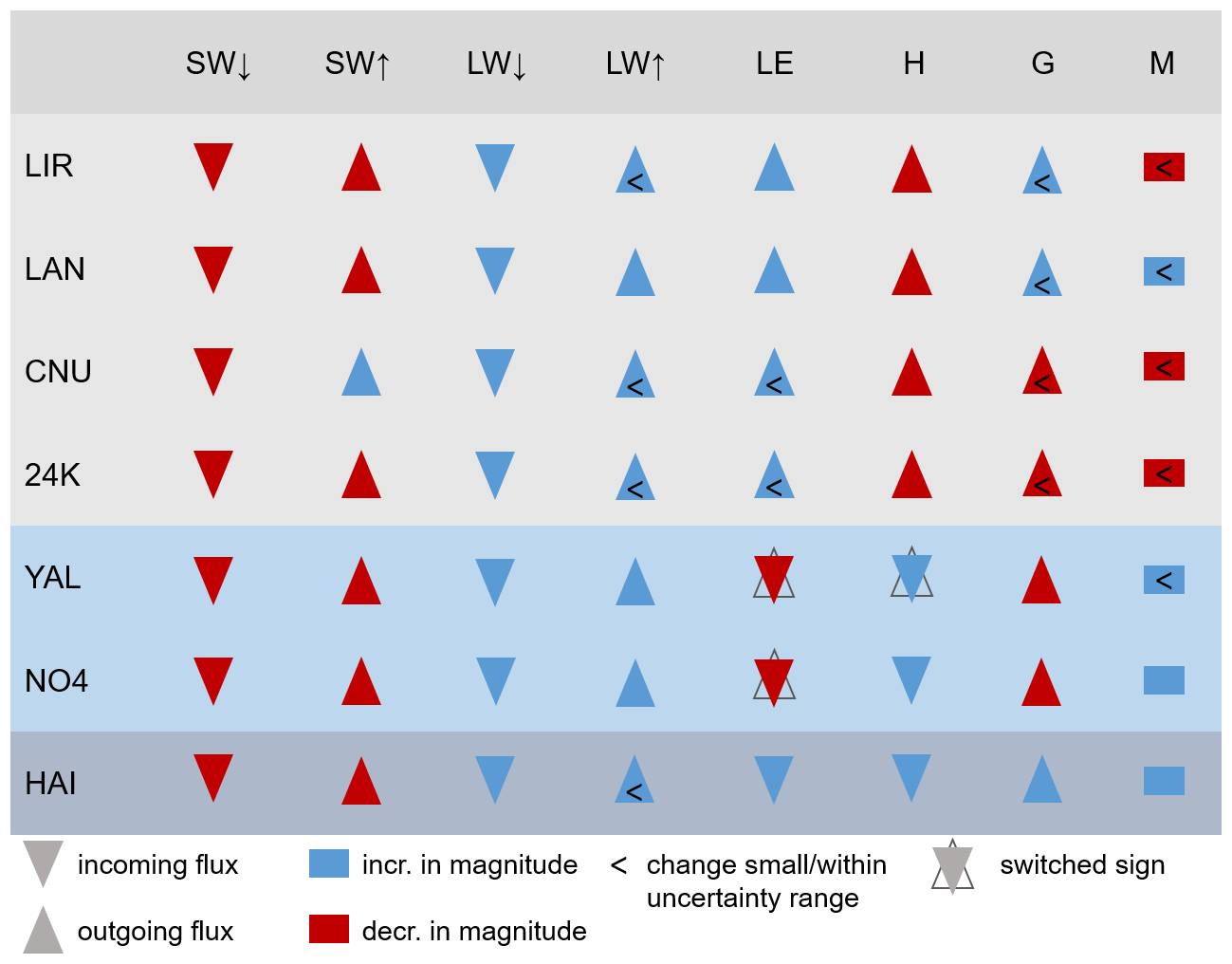
Figure 10Symbolic representation of changes in energy-balance components from pre-monsoon to monsoon. Triangles pointing down/up indicate a positive/negative flux with regard to our sign convention, where positive/negative means a flux towards/away from the surface, respectively. Red/blue indicate an increasing/decreasing value, respectively, of the flux when moving from pre-monsoon to monsoon. When signs switch, the underlying, empty triangles indicate the pre-monsoonal direction of the flux, while the overlying, coloured ones indicate the monsoonal flux.
5.4 Implications for Himalayan glaciers in a changing climate
Monsoon-influenced, summer-accumulation glaciers (such as Langtang, Lirung, Yala and Changri Nup) have been previously shown to be especially vulnerable to warming due to a decrease in accumulation and an enhancement of ablation due to reduced albedo (Fujita and Ageta, 2000), and our results confirm that SWnet is the key control on monsoon-period melt rates for clean-ice glaciers (Sect. 4.4.1). Our results also emphasise that the longevity of pre-monsoon snow cover into the monsoon period is a key control on melt rates (Sect. 4.1), supporting past findings that the strength and timing of the monsoon onset has a profound impact on small mountain glaciers (Mölg et al., 2014, 2012) through the phase change of precipitation in the transition to monsoon conditions (Fujita and Ageta, 2000; Ding et al., 2017; Zhu et al., 2018). Importantly, our insights into the differential response of glaciers with different surface types to the monsoon and its onset offer keys to interpret their future response under a changing climate:
All future climate scenarios agree on continued warming during the 21st century over High Mountain Asia (IPCC, 2021), together with a strengthening of elevation-dependent warming (Palazzi et al., 2017) and increases in moisture availability (IPCC, 2021). An analysis of the ensemble estimates of regionally downscaled CMIP5 projections (CORDEX) for the Himalaya (Sanjay et al., 2017) shows that total summer precipitation is projected to increase for the period 2036–2065 (2066–2095) by 4.4 % (10.5 %) in the Central Himalaya and by 6.8 % (10.4 %) in the Eastern Himalaya under RCP4.5 scenarios, relative to the period 1976–2005. While there is broad model consensus on the increase in future precipitation, there is little consensus on the future variability, frequency and spatial distribution of precipitation across High Mountain Asia (Kadel et al., 2018; Sanjay et al., 2017). A slight shift towards an earlier monsoon onset of <5 d over the coming century together with an increasing shift towards a later retreat by 5–10 d (mid-century) and 10–15 d (end-century) might increase the length of the monsoon period, with stronger lengthening in the Eastern Himalaya (Moon and Ha, 2020).
The prospect of warmer temperatures together with increased precipitation would (1) cause a shift in the precipitation partition from snow to rain in the monsoon, resulting in snow cover shifting to higher elevations and increasing total melt; (2) potentially lead to an increase in early spring snowfall, which would delay the onset of ice melt; (3) increase the likelihood of ephemeral monsoonal snow cover but move it to higher elevations, thus leaving more of the lower ablation zones exposed; and (4) increase the wet-bulb temperature together with humidity to result in a further reduction of the solid fraction of precipitation during monsoon. Overall it is likely that glacier ablation zones will be exposed for longer periods under future monsoon climate due to a net decrease of the snow covered duration, with a resulting increase in total ablation. A lengthening of the monsoon into autumn, on the other hand, Moon and Ha (2020) would somewhat offset warmer air temperatures with regard to the late-season melt for all glacier types.
The expected warmer and wetter monsoonal conditions, including increased cloudiness, will likely result in an overall increase of melt rates on clean-ice and glaciers with debris cover around or below the critical thickness. This is because (1) they are more directly controlled by net radiation (comprising both short- and long-wave fluxes), which is likely to increase in magnitude (Sect. 4.4.1); (2) the turbulent fluxes towards cold surfaces are also likely to increase in magnitude, and they tend to `work against' these types of glaciers (Sect. 4.4.1 and 4.4.3). Melt rates might increase to a lesser degree on debris-covered glaciers, since the turbulent fluxes `work for' the glaciers with debris above the critical thickness, and the melt-equalising effect of debris under monsoon (Sect. 4.4.2) might remain in place. These components could sum up to have an overall protective effect on glaciers with thick debris, allowing them to potentially resist the projected changes in the monsoonal summer longer into the future. Previous studies hypothesised that the mass balance of debris-covered glaciers might be less sensitive to climate warming compared with clean-ice glaciers (e.g. Anderson and Mackintosh, 2012; Wijngaard et al., 2019; Mattson, 2000). Here we additionally suggest that this difference in sensitivity could even be stronger in the monsoonal environments of the Central and Eastern Himalaya. Similarly, we suggest that glaciers with debris under the critical thickness might be even more sensitive to future monsoons than clean-ice glaciers. New energy-balance modelling studies incorporating similar datasets and future projections might provide answers to these still open questions.
5.5 Limitations
By applying an energy-balance model to seven sites across the Central and Eastern Himalaya, we have identified monsoon effects on the ablation season energy and mass balance of glaciers, common for the debris-covered and clean-ice glaciers studied here. A list of criteria used for choosing our modelling periods at each site is given in the Supplement Sect. S2. Applying these criteria, we chose one summer season record for each site, for which all required variables were available at a high level of data quality. As a result of this selection process, our analysis remained limited to one summer season at each site. Our work has also highlighted knowledge gaps which require further study: First, the influence of spring and monsoonal snow cover (its timing and amount) on the seasonal glacier mass balance is currently difficult to discern due to the paucity of multi-annual datasets in High Mountain Asia. Second, the timing and quantity of post-monsoon and winter precipitation influence the annual mass balance; however, even fewer datasets exist for the winter half-year in HMA, preventing a year-round analysis of similar detail. Third, all our sites are located in glacier ablation areas, and surface and energy mass fluxes will change with elevation. While we have tested how representative our point-scale results are for the entire ablation area of the glaciers considered, the response of glacier accumulation areas to monsoon remains to be investigated. Meteorological data from accumulation areas are scarce, however, limiting our current understanding. Future work should establish new year-round and multi-year records, including datasets from accumulation areas, in order to extend some of our findings. Future work could also target the spatial distribution of forcing data and parameters necessary to run energy-balance models at the glacier scale.
We model the energy and mass balance of seven glaciers in the Central and Eastern Himalaya at seven on-glacier weather stations. We find that:
-
At all sites, the largest mass loss component during the ablation season is ice melt, followed by snowmelt and sublimation, while the latter only plays a role at our highest sites and outside of the core monsoon. We find that the seasonal energy and mass balance is strongly controlled by variations of absorbed shortwave radiation, a result of the prevalence of spring snow cover and the occurrence of ephemeral monsoonal snow accumulation.
-
Debris cover above the critical thickness returns most of the energy it absorbs back to the atmosphere via longwave emission and turbulent heat fluxes. While H is primarily controlled by the temperature gradient between surface and air, LE is controlled by the availability of liquid water at the debris surface. When debris is around or under the critical thickness, the melt is more directly radiation-driven. In this case, however, melt is additionally increased by the turbulent fluxes H and LE, for which wind speed is the primary control. The cold surface favours condensation rather than evaporation as well as sensible heat exchange into the glacier surface.
-
The response of the glacier mass and energy balance to the monsoon depends on the surface type: Melt rates tend to increase compared to the pre-monsoon at the clean-ice glaciers and the glacier with thin debris cover (with the exception of Yala), while they stay similar at the glaciers with thick debris cover. We attribute these differences to the role the turbulent fluxes play for each surface type. At the glaciers with thick debris cover, where the turbulent fluxes `work for' the glacier, evaporation of the additionally available moisture (LE) provides extra cooling during the monsoon. The evaporation of liquid water is a moisture limited process during the pre-monsoon and turns into an energy-limited process during the monsoon. The monsoonal decrease in SW↓ is further offset by an increase in LW↓ and a decrease in cooling induced by H, with the result of unchanged available melt energy M during monsoon. In a sensitivity experiment, we confirm that these results are representative of the entire ablation zones of the thickly debris-covered glaciers. At the clean-ice sites, by contrast, the melt is mostly radiation controlled throughout the ablation season and varies greatly over the elevation profile of the ablation zone. The turbulent fluxes play a subordinate role there, but can switch from melt-reducing to melt-enhancing in the seasonal transition into the monsoon. At the thin debris-covered site, on the other hand, the turbulent fluxes always `work against' the glacier and intensify during the monsoon.
Given these findings, under projected future monsoonal conditions, namely warmer and possibly longer and wetter monsoons (Sanjay et al., 2017; Moon and Ha, 2020; IPCC, 2021), the summer season mass balance of glaciers with thick debris cover might react less sensitively than the one of clean-ice glaciers and glaciers with thin debris. We encourage future research to answer this still open question.
All AWS datasets for the modelling periods considered in the analysis, together with ablation measurements, pre-processed forcing data, T&C model codes, outputs and scripts for analysing outputs are available under the following link: https://doi.org/10.5281/zenodo.6280986 (Fugger et al., 2022). When previously published elsewhere, references and links to the full, original datasets are provided in the data repository.
The supplement related to this article is available online at: https://doi.org/10.5194/tc-16-1631-2022-supplement.
StF, FP and EM designed the study. StF carried out the analysis with the help of CLF, MM and SiF. StF interpreted the results, created the figures and wrote the paper with the help of CLF, EM, MM, TES and FP. SiF, PW, WI, and QL reviewed the paper. WY and BD facilitated field data collection and provided parameterisations for albedo and precipitation phase. WY, PW and WI also contributed datasets.
The contact author has declared that neither they nor their co-authors have any competing interests.
Publisher's note: Copernicus Publications remains neutral with regard to jurisdictional claims in published maps and institutional affiliations.
We would like to thank our four anonymous reviewers, who's comments greatly helped to improve the paper. We would also like to thank Jakob Steiner and ICIMOD for hosting and contributing datasets. Our special thanks go to Marin Kneib for organising the field campaigns, and the Langtang and 24K field teams for making the data collection possible.
This research has been supported by the European Research Council, H2020 European Research Council (RAVEN (grant no. 772751)). The National Natural Science Foundation of China (41961134035) financially supported the data collection on 24K and Parlung No.4 glaciers.
This paper was edited by Marie Dumont and reviewed by four anonymous referees.
Aizen, V., Aizen, E., and Nikitin, S.: Glacier regime on the northern slope of the Himalaya (Xixibangma glaciers), Quatern. Int., 97, 27–39, 2002. a
Anderson, B. and Mackintosh, A.: Controls on mass balance sensitivity of maritime glaciers in the Southern Alps, New Zealand: the role of debris cover, J. Geophys. Res.-Earth, 117, https://doi.org/10.1029/2011JF002064, 2012. a
Azam, M. F., Wagnon, P., Vincent, C., Ramanathan, AL., Favier, V., Mandal, A., and Pottakkal, J. G.: Processes governing the mass balance of Chhota Shigri Glacier (western Himalaya, India) assessed by point-scale surface energy balance measurements, The Cryosphere, 8, 2195–2217, https://doi.org/10.5194/tc-8-2195-2014, 2014. a
Bélair, S., Crevier, L.-P., Mailhot, J., Bilodeau, B., and Delage, Y.: Operational implementation of the ISBA land surface scheme in the Canadian regional weather forecast model. Part I: Warm season results, J. Hydrometeorol., 4, 352–370, 2003. a, b
Bonekamp, P. N., de Kok, R. J., Collier, E., and Immerzeel, W. W.: Contrasting meteorological drivers of the glacier mass balance between the Karakoram and central Himalaya, Front. Earth Sci., 7, https://doi.org/10.3389/feart.2019.00107, 2019. a, b, c, d, e
Bookhagen, B. and Burbank, D. W.: Toward a complete Himalayan hydrological budget: Spatiotemporal distribution of snowmelt and rainfall and their impact on river discharge, J. Geophys. Res.-Earth, 115, https://doi.org/10.1029/2009JF001426, 2010. a
Botter, M., Zeeman, M., Burlando, P., and Fatichi, S.: Impacts of fertilization on grassland productivity and water quality across the European Alps under current and warming climate: insights from a mechanistic model, Biogeosciences, 18, 1917–1939, https://doi.org/10.5194/bg-18-1917-2021, 2021. a
Brock, B. W., Willis, I. C., and Sharp, M. J.: Measurement and parameterization of albedo variations at Haut Glacier d’Arolla, Switzerland, J. Glaciol., 46, 675–688, 2000. a
Brun, F., Berthier, E., Wagnon, P., Kääb, A., and Treichler, D.: A spatially resolved estimate of High Mountain Asia glacier mass balances from 2000 to 2016, Nat. Geosci., 10, 668–673, 2017. a
Collier, E. and Immerzeel, W. W.: High-resolution modeling of atmospheric dynamics in the Nepalese Himalaya, J. Geophys. Res.-Atmos., 120, 9882–9896, 2015. a, b
Collier, E., Nicholson, L. I., Brock, B. W., Maussion, F., Essery, R., and Bush, A. B. G.: Representing moisture fluxes and phase changes in glacier debris cover using a reservoir approach, The Cryosphere, 8, 1429–1444, https://doi.org/10.5194/tc-8-1429-2014, 2014. a, b, c
Collier, E., Maussion, F., Nicholson, L. I., Mölg, T., Immerzeel, W. W., and Bush, A. B. G.: Impact of debris cover on glacier ablation and atmosphere–glacier feedbacks in the Karakoram, The Cryosphere, 9, 1617–1632, https://doi.org/10.5194/tc-9-1617-2015, 2015. a, b
Cuffey, K. M. and Paterson, W. S. B.: The physics of glaciers, Academic Press, 4th Edition, ISBN 9780123694614, 2010. a
Ding, B., Yang, K., Qin, J., Wang, L., Chen, Y., and He, X.: The dependence of precipitation types on surface elevation and meteorological conditions and its parameterization, J. Hydrol., 513, 154–163, 2014. a, b
Ding, B., Yang, K., Yang, W., He, X., Chen, Y., Guo, X., Wang, L., Wu, H., and Yao, T.: Development of a Water and Enthalpy Budget-based Glacier mass balance Model (WEB-GM) and its preliminary validation, Water Resour. Res., 53, 3146–3178, 2017. a, b
Evatt, G. W., Abrahams, I. D., Heil, M., Mayer, C., Kingslake, J., Mitchell, S. L., Fowler, A. C., and Clark, C. D.: Glacial melt under a porous debris layer, J. Glaciol., 61, 825–836, 2015. a, b, c, d, e, f
Farinotti, D., Huss, M., Fürst, J. J., Landmann, J., Machguth, H., Maussion, F., and Pandit, A.: A consensus estimate for the ice thickness distribution of all glaciers on Earth, Nat. Geosci., 12, 168–173, 2019. a
Farinotti, D., Immerzeel, W. W., de Kok, R. J., Quincey, D. J., and Dehecq, A.: Manifestations and mechanisms of the Karakoram glacier Anomaly, Nat. Geosci., 13, 8–16, 2020. a
Fatichi, S., Ivanov, V. Y., and Caporali, E.: A mechanistic ecohydrological model to investigate complex interactions in cold and warm water-controlled environments: 1. Theoretical framework and plot-scale analysis, J. Adv. Model. Earth Sys., 4, https://doi.org/10.1029/2011MS000086, 2012. a
Fugger, S., Fyffe, C., Fatichi, S., Miles, E., McCarthy, M., Shaw, T. E., Ding, B., Yang, W., Wagnon, P., Immerzee, W., and Liu, Q.: Understanding monsoon controls on the energy and mass balance of glaciers in the Central and Eastern Himalaya, Zenodo [data set and code], https://doi.org/10.5281/zenodo.6280986, 2022. a
Fujita, K. and Ageta, Y.: Effect of summer accumulation on glacier mass balance on the Tibetan Plateau revealed by mass-balance model, J. Glaciol., 46, 244–252, 2000. a, b, c, d
Fujita, K. and Sakai, A.: Modelling runoff from a Himalayan debris-covered glacier, Hydrol. Earth Syst. Sci., 18, 2679–2694, https://doi.org/10.5194/hess-18-2679-2014, 2014. a
Fujita, K., Takeuchi, N., and Seko, K.: Glaciological observations of Yala Glacier in Langtang Valley, Nepal Himalayas, 1994 and, B. Glacier Res., 16, 75–8, 1998. a, b
Fyffe, C. L., Woodget, A. S., Kirkbride, M. P., Deline, P., Westoby, M. J., and Brock, B. W.: Processes at the margins of supraglacial debris cover: quantifying dirty ice ablation and debris redistribution, Earth Surf. Proc. Land., 45, 2272–2290, https://doi.org/10.1002/esp.4879, 2020. a
Gardelle, J., Berthier, E., and Arnaud, Y.: Slight mass gain of Karakoram glaciers in the early twenty-first century, Nat. Geosci., 5, 322–325, 2012. a
Giese, A., Boone, A., Wagnon, P., and Hawley, R.: Incorporating moisture content in surface energy balance modeling of a debris-covered glacier, The Cryosphere, 14, 1555–1577, https://doi.org/10.5194/tc-14-1555-2020, 2020. a, b
Herreid, S. and Pellicciotti, F.: The state of rock debris covering Earth’s glaciers, Nat. Geosci., 13, 621–627, https://doi.org/10.1038/s41561-020-0615-0, 2020. a, b
Heynen, M., Miles, E., Ragettli, S., Buri, P., Immerzeel, W. W., and Pellicciotti, F.: Air temperature variability in a high-elevation Himalayan catchment, Ann. Glaciol., 57, 212–222, 2016. a
ICIMOD RDS database: AWS Yala Glacier, ICIMOD [data set], https://doi.org/10.26066/RDS.1972507, 2021. a
Immerzeel, W. W., Van Beek, L., Konz, M., Shrestha, A., and Bierkens, M.: Hydrological response to climate change in a glacierized catchment in the Himalayas, Climatic Change, 110, 721–736, 2012. a
Immerzeel, W. W., Kraaijenbrink, P. D., Shea, J., Shrestha, A. B., Pellicciotti, F., Bierkens, M. F., and de Jong, S. M.: High-resolution monitoring of Himalayan glacier dynamics using unmanned aerial vehicles, Remote Sens. Environ., 150, 93–103, 2014. a
IPCC: Climate Change 2021: The Physical Science Basis. Contribution of Working Group I to the Sixth Assessment Report of the Intergovernmental Panel on Climate Change, edited by: Masson-Delmotte, V., Zhai, P., Pirani, A., Connors, S. L., Péan, C., Berger, S., Caud, N., Chen, Y., Goldfarb, L., Gomis, M. I., Huang, M., Leitzell, K., Lonnoy, E., Matthews, J. B. R., Maycock, T. K., Waterfield, T., Yelekçi, O., Yu, R., and Zhou, B., Cambridge University Press, in press, 2021. a, b, c
Kadel, I., Yamazaki, T., Iwasaki, T., and Abdillah, M. R.: Projection of future monsoon precipitation over the central Himalayas by CMIP5 models under warming scenarios, Clim. Res., 75, 1–21, 2018. a
Kaser, G., Großhauser, M., and Marzeion, B.: Contribution potential of glaciers to water availability in different climate regimes, P. Natl. Acad. Sci. USA, 107, 20223–20227, 2010. a
Kayastha, R. B., Ohata, T., and Ageta, Y.: Application of a mass-balance model to a Himalayan glacier, J. Glaciol., 45, 559–567, 1999. a
Kraaijenbrink, P., Bierkens, M., Lutz, A., and Immerzeel, W.: Impact of a global temperature rise of 1.5 degrees Celsius on Asia’s glaciers, Nature, 549, 257–260, 2017. a, b
Kumar, K. K., Rajagopalan, B., Hoerling, M., Bates, G., and Cane, M.: Unraveling the mystery of Indian monsoon failure during El Niño, Science, 314, 115–119, 2006. a
Lejeune, Y., Bertrand, J.-M., Wagnon, P., and Morin, S.: A physically based model of the year-round surface energy and mass balance of debris-covered glaciers, J. Glaciol., 59, 327–344, 2013. a, b, c, d, e
Liao, H., Liu, Q., Zhong, Y., and Lu, X.: Landsat-based estimation of the glacier surface temperature of Hailuogou glacier, Southeastern Tibetan Plateau, between 1990 and 2018, Remote Sensing, 12, 2105, https://doi.org/10.3390/rs12132105, 2020. a
Luo, L.: Basic meteorological data of glacier moraine area at 24K in Galongla, Southeast Tibet station, Chinese Academy of Sciences (2018–2019), National Tibetan Plateau Data Center [data set], https://doi.org/18406.11.Meteoro.tpdc.271131, 2020. a, b
Mascart, P., Noilhan, J., and Giordani, H.: A modified parameterization of flux-profile relationships in the surface layer using different roughness length values for heat and momentum, Bound.-Lay. Meteorol., 72, 331–344, 1995. a
Mastrotheodoros, T., Pappas, C., Molnar, P., Burlando, P., Manoli, G., Parajka, J., Rigon, R., Szeles, B., Bottazzi, M., Hadjidoukas, P., and Fatichi, S.: More green and less blue water in the Alps during warmer summers, Nat. Clim. Change, 10, 155–161, 2020. a
Mattson, L. E.: The influence of a debris cover on the mid-summer discharge of Dome Glacier, Canadian Rocky Mountains, IAHS-AISH Publication, 25–34, 2000. a
Maussion, F., Scherer, D., Mölg, T., Collier, E., Curio, J., and Finkelnburg, R.: Precipitation seasonality and variability over the Tibetan Plateau as resolved by the High Asia Reanalysis, J. Climate, 27, 1910–1927, 2014. a, b
McCarthy, M. J.: Quantifying supraglacial debris thickness at local to regional scales, PhD thesis, Scott Polar Research Institute and British Antarctic Survey, 2018. a, b
Miles, E. S., Steiner, J. F., and Brun, F.: Highly variable aerodynamic roughness length (z0) for a hummocky debris-covered glacier, J. Geophys. Res.-Atmos., 122, 8447–8466, 2017. a, b
Mölg, T., Maussion, F., Yang, W., and Scherer, D.: The footprint of Asian monsoon dynamics in the mass and energy balance of a Tibetan glacier, The Cryosphere, 6, 1445–1461, https://doi.org/10.5194/tc-6-1445-2012, 2012. a, b, c, d, e, f
Mölg, T., Maussion, F., and Scherer, D.: Mid-latitude westerlies as a driver of glacier variability in monsoonal High Asia, Nat. Clim. Change, 4, 68–73, 2014. a, b, c, d, e
Moon, S. and Ha, K.-J.: Future changes in monsoon duration and precipitation using CMIP6, npj Clim. Atmos. Sci., 3, 1–7, 2020. a, b, c
Muñoz Sabater, J.: ERA5-Land monthly averaged data from 1981 to present Copernicus Climate Change Service (C3S) Climate Data Store (CDS), https://doi.org/10.24381/cds.68d2bb30, 2019. a
Nakawo, M. and Rana, B.: Estimate of ablation rate of glacier ice under a supraglacial debris layer, Geogr. Ann. A, 81, 695–701, 1999. a, b, c
Nicholson, L. and Benn, D. I.: Calculating ice melt beneath a debris layer using meteorological data, J. Glaciol., 52, 463–470, 2006. a, b, c, d
Noilhan, J. and Mahfouf, J.-F.: The ISBA land surface parameterisation scheme, Global Planet. Change, 13, 145–159, 1996. a
Östrem, G.: Ice melting under a thin layer of moraine, and the existence of ice cores in moraine ridges, Geogr. Ann., 41, 228–230, 1959. a, b, c
Palazzi, E., Filippi, L., and von Hardenberg, J.: Insights into elevation-dependent warming in the Tibetan Plateau-Himalayas from CMIP5 model simulations, Clim. Dynam., 48, 3991–4008, 2017. a
Paschalis, A., Fatichi, S., Pappas, C., and Or, D.: Covariation of vegetation and climate constrains present and future T/ET variability, Environ. Res. Lett., 13, 104012, https://doi.org/10.1088/1748-9326/aae267, 2018. a
Pratap, B., Dobhal, D., Mehta, M., and Bhambri, R.: Influence of debris cover and altitude on glacier surface melting: a case study on Dokriani Glacier, central Himalaya, India, Ann. Glaciol., 56, 9–16, 2015. a
Quincey, D., Smith, M., Rounce, D., Ross, A., King, O., and Watson, C.: Evaluating morphological estimates of the aerodynamic roughness of debris covered glacier ice, Earth Surf. Proc. Land., 42, 2541–2553, 2017. a, b
Ragettli, S., Pellicciotti, F., Immerzeel, W. W., Miles, E. S., Petersen, L., Heynen, M., Shea, J. M., Stumm, D., Joshi, S., and Shrestha, A.: Unraveling the hydrology of a Himalayan catchment through integration of high resolution in situ data and remote sensing with an advanced simulation model, Adv. Water Resour., 78, 94–111, 2015. a, b
Reid, T. D. and Brock, B. W.: An energy-balance model for debris-covered glaciers including heat conduction through the debris layer, J. Glaciol., 56, 903–916, 2010. a, b, c, d, e, f, g
Reznichenko, N., Davies, T., Shulmeister, J., and McSaveney, M.: Effects of debris on ice-surface melting rates: an experimental study, J. Glaciol., 56, 384–394, 2010. a, b, c
Rounce, D. R., Quincey, D. J., and McKinney, D. C.: Debris-covered glacier energy balance model for Imja–Lhotse Shar Glacier in the Everest region of Nepal, The Cryosphere, 9, 2295–2310, https://doi.org/10.5194/tc-9-2295-2015, 2015. a, b, c, d
Rowan, A. V., Nicholson, L. I., Quincey, D. J., Gibson, M. J., Irvine-Fynn, T. D., Watson, C. S., Wagnon, P., Rounce, D. R., Thompson, S. S., Porter, P. R., and Glasser, N. F.: Seasonally stable temperature gradients through supraglacial debris in the Everest region of Nepal, Central Himalaya, J. Glaciol., 67, 170–181, https://doi.org/10.1017/jog.2020.100, 2020. a, b
Sakai, A. and Fujita, K.: Contrasting glacier responses to recent climate change in high-mountain Asia, Sci. Rep., 7, 1–8, 2017. a
Sakai, A., Fujita, K., and Kubota, J.: Evaporation and percolation effect on melting at debris-covered Lirung Glacier, Nepal Himalayas, 1996, B. Glaciol. Res., 21, 9–16, 2004. a, b
Sanjay, J., Krishnan, R., Shrestha, A. B., Rajbhandari, R., and Ren, G.-Y.: Downscaled climate change projections for the Hindu Kush Himalayan region using CORDEX South Asia regional climate models, Adv. Clim. Change Res., 8, 185–198, 2017. a, b, c
Scherler, D., Bookhagen, B., and Strecker, M. R.: Hillslope-glacier coupling: The interplay of topography and glacial dynamics in High Asia, J. Geophys. Res.-Earth, 116, https://doi.org/10.1029/2010JF001751, 2011a. a
Scherler, D., Bookhagen, B., and Strecker, M. R.: Spatially variable response of Himalayan glaciers to climate change affected by debris cover, Nat. Geosci., 4, 156–159, 2011b. a, b
Shah, S. S., Banerjee, A., Nainwal, H. C., and Shankar, R.: Estimation of the total sub-debris ablation from point-scale ablation data on a debris-covered glacier, J. Glaciol., 65, 759–769, 2019. a
Shean, D., Bhushan, S., Montesano, P., Rounce, D., Arendt, A., and Osmanoglu, B.: A systematic, regional assessment of High Mountain Asia Glacier mass balance, Front. Earth Sci., 7, 363, https://doi.org/10.3389/feart.2019.00363, 2020. a
Shrestha, R., Kayastha, R., and Kayastha, R.: Effect of debris on seasonal ice melt (2016–2018) on Ponkar Glacier, Manang, Nepal, Sci. Cold Arid Reg., 12, 261–271, 2020. a
Steiner, J. F. and Pellicciotti, F.: Variability of air temperature over a debris-covered glacier in the Nepalese Himalaya, Ann. Glaciol., 57, 295–307, 2016. a
Steiner, J. F., Litt, M., Stigter, E. E., Shea, J., Bierkens, M. F., and Immerzeel, W. W.: The importance of turbulent fluxes in the surface energy balance of a debris-covered glacier in the Himalayas, Front. Earth Sci., 6, 144, https://doi.org/10.3389/feart.2018.00144, 2018. a, b, c, d, e, f
Stumm, D., Joshi, S. P., Gurung, T. R., and Silwal, G.: Mass balances of Yala and Rikha Samba glaciers, Nepal, from 2000 to 2017, Earth Syst. Sci. Data, 13, 3791–3818, https://doi.org/10.5194/essd-13-3791-2021, 2021. a
Sun, W., Qin, X., Du, W., Liu, W., Liu, Y., Zhang, T., Xu, Y., Zhao, Q., Wu, J., and Ren, J.: Ablation modeling and surface energy budget in the ablation zone of Laohugou glacier No. 12, western Qilian mountains, China, Ann. Glaciol., 55, 111–120, 2014. a, b
van den Broeke, M., van As, D., Reijmer, C., and van de Wal, R.: Assessing and improving the quality of unattended radiation observations in Antarctica, J. Atmos. Ocean. Tech., 21, 1417–1431, 2004. a
Verseghy, D. L.: CLASS – A Canadian land surface scheme for GCMs. I. Soil model, Int. J. Climatol., 11, 111–133, 1991. a
Vincent, C., Wagnon, P., Shea, J. M., Immerzeel, W. W., Kraaijenbrink, P., Shrestha, D., Soruco, A., Arnaud, Y., Brun, F., Berthier, E., and Sherpa, S. F.: Reduced melt on debris-covered glaciers: investigations from Changri Nup Glacier, Nepal, The Cryosphere, 10, 1845–1858, https://doi.org/10.5194/tc-10-1845-2016, 2016. a
Wagnon, P.: IACS working group on debris-covered glaciers, AWS North Changri Nup Glacier [data set], https://glacioclim.osug.fr/IACS-working-group-on-debris-covered-glaciers-Data (last access: 1 April 2022), 2021. a
Wijngaard, R. R., Steiner, J. F., Kraaijenbrink, P. D., Klug, C., Adhikari, S., Banerjee, A., Pellicciotti, F., Van Beek, L. P., Bierkens, M. F., Lutz, A. F., and Immerzeel, W. W.: Modeling the Response of the Langtang Glacier and the Hintereisferner to a Changing Climate Since the Little Ice Age, Front. Earth Sci., 7, https://doi.org/10.3389/feart.2019.00143, 2019. a
Yang, W., Guo, X., Yao, T., Yang, K., Zhao, L., Li, S., and Zhu, M.: Summertime surface energy budget and ablation modeling in the ablation zone of a maritime Tibetan glacier, J. Geophys. Res.-Atmos., 116, https://doi.org/10.1029/2010JD015183, 2011. a, b
Yang, W., Yao, T., Zhu, M., and Wang, Y.: Comparison of the meteorology and surface energy fluxes of debris-free and debris-covered glaciers in the southeastern Tibetan Plateau, J. Glaciol., 63, 1090–1104, 2017. a, b, c, d, e, f, g, h, i
Yao, T., Thompson, L., Yang, W., Yu, W., Gao, Y., Guo, X., Yang, X., Duan, K., Zhao, H., Xu, B., and Pu, J.: Different glacier status with atmospheric circulations in Tibetan Plateau and surroundings, Nat. Clim. Change, 2, 663–667, 2012. a, b, c, d
Zhang, Y., Fujita, K., Liu, S., Liu, Q., and Nuimura, T.: Distribution of debris thickness and its effect on ice melt at Hailuogou glacier, southeastern Tibetan Plateau, using in situ surveys and ASTER imagery, J. Glaciol., 57, 1147–1157, 2011. a
Zhu, M., Yao, T., Yang, W., Xu, B., Wu, G., and Wang, X.: Differences in mass balance behavior for three glaciers from different climatic regions on the Tibetan Plateau, Clim. Dynam., 50, 3457–3484, 2018. a, b, c, d, e