the Creative Commons Attribution 4.0 License.
the Creative Commons Attribution 4.0 License.
 | 12 Apr 2022
Mass evolution of the Antarctic Peninsula over the last 2 decades from a joint Bayesian inversion
Andrew Zammit-Mangion
Jonathan Rougier
Geoffrey Dawson
Jonathan L. Bamber
The Antarctic Peninsula has become an increasingly important component of the Antarctic Ice Sheet mass budget over the last 2 decades, with mass losses generally increasing. However, due to the challenges presented by the topography and geometry of the region, there remain large variations in mass balance estimates from conventional approaches and in assessing the relative contribution of individual ice sheet processes. Here, we use a regionally optimized Bayesian hierarchical model joint inversion approach that combines data from multiple altimetry studies (ENVISAT, ICESat, CryoSat-2 swath), gravimetry (GRACE and GRACE-FO), and localized DEM differencing observations to solve for annual mass trends and their attribution to individual driving processes for the period 2003–2019. This is first time that such localized observations have been assimilated directly to estimate mass balance as part of a wider-scale regional assessment. The region experienced a mass imbalance rate of Gt yr−1 between 2003 and 2019, predominantly driven by accelerations in ice dynamic mass losses in the first decade and sustained thereafter. Inter-annual variability is driven by surface processes, particularly in 2016 due to increased precipitation driven by an extreme El Niño, which temporarily returned the sector back to a state of positive mass balance. In the West Palmer Land and the English Coast regions, surface processes are a greater contributor to mass loss than ice dynamics in the early part of the 2010s. Our results show good agreement with conventional and other combination approaches, improving confidence in the robustness of mass trend estimates, and in turn, understanding of the region's response to changes in external forcing.
- Article
(4370 KB) - Full-text XML
-
Supplement
(12534 KB) - BibTeX
- EndNote


Over the last 2 decades, the Antarctic Peninsula (AP) and Bellingshausen Sea sector of West Antarctica have experienced increased mass loss (Martín-Español et al., 2016; McMillan et al., 2014; Sutterley et al., 2014; Wouters et al., 2015), grounding line migration (Christie et al., 2016), and increases in ice sheet velocity (Gardner et al., 2018; Mouginot et al., 2014). The collapse of the Larsen A and near-full collapse of Larsen B ice shelves in 1995 and 2002, respectively, and the subsequent reduction in buttressing they provide to the grounded ice sheet, resulted in rapid thinning (Rott et al., 2018; Scambos et al., 2014) and increased glacier flow velocities (Scambos et al., 2004) in the northern AP. These events are seen as potential analogues for a future response of the West Antarctic Ice Sheet (WAIS) to further ice shelf thinning or collapse, particularly over areas susceptible to marine ice sheet instability (Schoof, 2007). Continuous long-term monitoring of the AP is important as it can help us better understand the multi-decadal ice sheet response to external oceanic and atmospheric forcing, subsequently improving process representation in ice sheet models. Additionally, the AP has accounted for an increasingly significant component of the ice sheet's contribution to global sea level rise over recent decades (Bamber et al., 2018; WCRP Global Sea Level Budget Group, 2018; Shepherd et al., 2018). Robust estimates of its mass changes are imperative to provide sea-level budget closure. The AP is difficult to monitor using conventional mass balance approaches. The high relief of the peninsula makes it a particularly poor region to monitor with satellite altimetry, interferometric SAR-derived (InSAR) velocities, and ice thickness data. In addition, the sharp topography and large climatic gradient across the AP provide significant challenges for regional climate models. Finally, the more northerly latitude increases the across-track spacing between orbits for satellite altimetry, which decreases the available measurements in the region.
These coverage issues have made it difficult to reconcile mass balance estimates for the AP from conventional approaches, with altimetry and mass budget techniques not agreeing within error for the period 2003–2010 (Shepherd et al., 2018). At the individual basin scale, even estimates from the conventional approaches using the same observations do not agree within error for common time periods (McMillan et al., 2014; Wouters et al., 2015). This suggests uncertainties and biases in the methodological assumptions and model corrections are being propagated into the resulting mass balance estimates. By contrast, data-driven approaches which can simultaneously assimilate the diverse observations available allow us to exploit their individual advantages, whilst reducing the sources of uncertainty and assumptions required by single-technique approaches (Martin-Español et al., 2016). Robustly combining these observations, however, is challenging due to their markedly different spatio-temporal characteristics and sources of common error.
To address this issue, we apply a Bayesian hierarchical model (BHM) framework (Zammit-Mangion et al., 2014, 2015a, b) to resolve for the spatio-temporal mass trends and component parts for the AP from 2003 to 2019, an approach which has been previously demonstrated at the ice sheet scale for a shorter time period (Martín-Español et al., 2016). We develop and optimize the BHM framework for this high-relief region of Antarctica by both improving the spatial resolution and including new observation datasets. An advantage of the BHM approach is its ability to incorporate irregular data in both space and time, while explicitly accounting for error propagation in the results. This means we can exploit localized datasets such as elevation change from high-resolution digital elevation model differencing (dDEM), as well as addressing the gap in the gravimetry record between the decommissioning of GRACE in 2017 and the launch of GRACE-FO in 2018. The combination of a diverse range of observations enables us to constrain the mass balance of the region with high confidence and provide insights into the driving processes. We use these mass trend estimates and their component parts to explore the discrepancies between different approaches for the West Palmer Land region in the southern AP, one of the most challenging regions of the ice sheet to observe and the source of the greatest divergence in previous mass balance estimates.
For the 2003 to 2019 period of this study, observations of ice sheet elevation and mass change from multiple missions are used as inputs to the BHM framework. The spatial domain of our study is shown in Fig. 1a, with altimetry dataset coverage shown in Fig. 1b and region specific datasets for the northern AP in Fig. 1c. An overview of datasets in the framework is additionally given in Table 1. As our framework solves for the rate of elevation change in each ice sheet process at a calendar year resolution, our datasets represent the rate of change in either elevation or mass. All datasets are processed to represent calendar year trends, with differing methodological approaches given the variations in the spatio-temporal sampling of each dataset. All datasets were then converted to a common Antarctic Polar Stereographic Projection (EPSG:3031). The sections below focus on the processing methodologies for each category of observation.
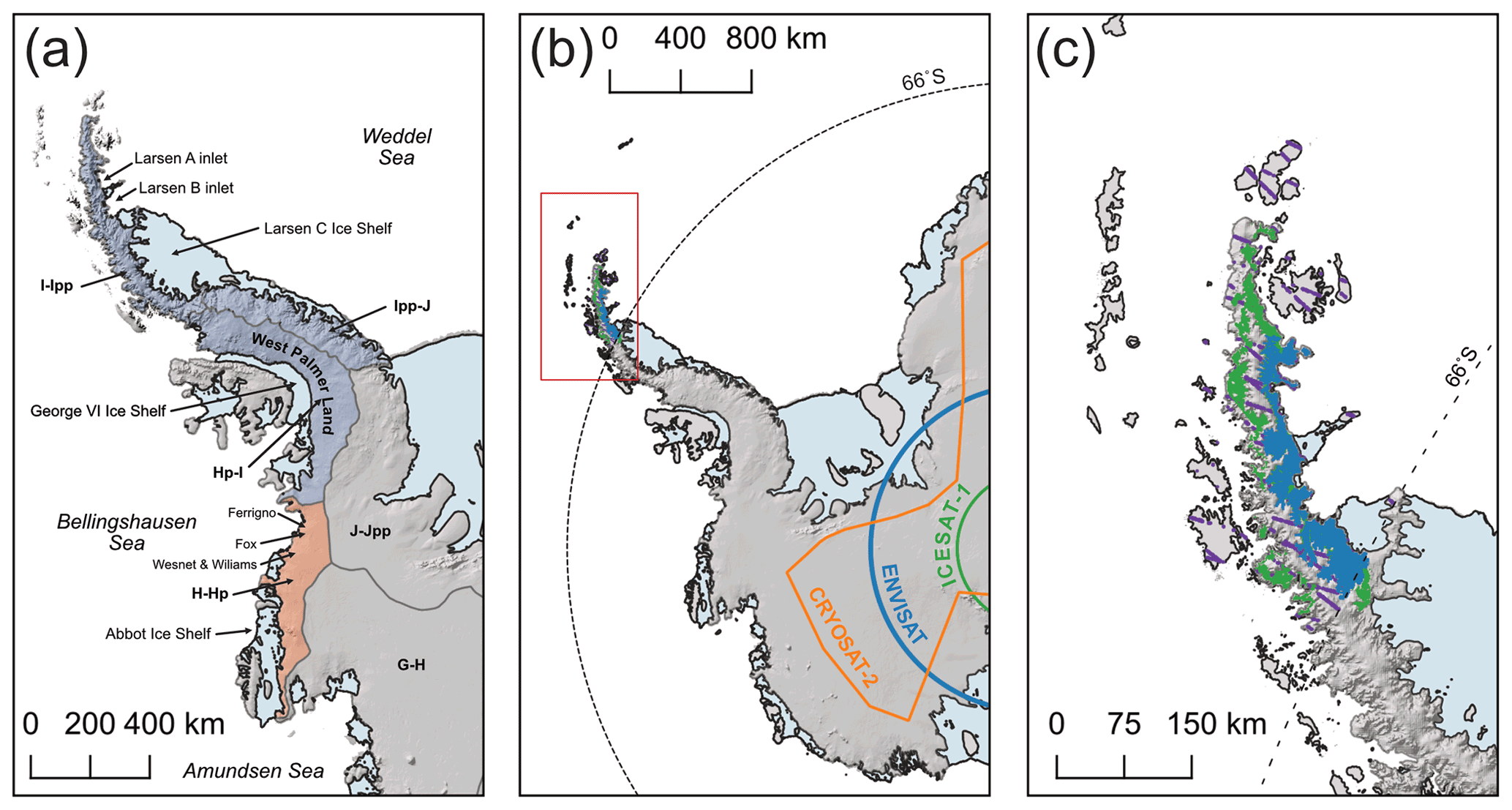
Figure 1(a) Region of interest for this study, overlain with drainage basin definitions (Rignot et al., 2011b, 2013). Basins included in the Ice Sheet Mass Balance Intercomparison Exercise (IMBIE) (Shepherd et al., 2018) definition of the AP are shaded in purple, with orange basins indicating those outside the AP but included in this study. (b) Spatial coverage of altimetry and DEM datasets for the region. The latitudinal limits of ICESat and ENVISAT are shown in green and blue, respectively. The orange line indicates the CryoSat-2 POCA/swath to low-resolution mode (LRM) transition (with LRM coverage south of the orange delineation). The dashed latitudinal line at 66∘ S indicates the separation between ICESat data used over the interior of the ice sheet (Martín-Español et al., 2016) and the optimized data over the northern AP (Scambos et al., 2014). (c) Zoomed spatial coverage of the red bounding box in (b), indicating the datasets used over the northern AP. Purple and green regions indicate coverage of the optimized ICESat data and dDEM data, respectively, from Scambos et al. (2014). Blue regions indicate coverage of dDEM data from Rott et al. (2018). All data are overlain on the hill shade of the reference elevation model of Antarctica REMA DEM (Howat et al., 2019).
Table 1Summary of observations and prior auxiliary datasets used in this study, including their spatio-temporal coverage and latent processes they observe.

n/a: not applicable.
2.1 Gravimetry
In this study we use the NASA Jet Propulsion Laboratory (JPL) RL06_v02 global monthly mascon product to provide observations of mass change from the GRACE and GRACE-FO mission for the time period 2003 to 2019 (Landerer et al., 2020; Watkins et al., 2015; Wiese et al., 2016, 2018). The dataset consists of monthly mass change anomalies with respect to a 2004–2009 time-mean baseline, posted on a global grid interpolated from equal-area 3∘ diameter spherical caps. We use the product which has not been processed using the Coastline Resolution Improvement (CRI) filter, as the BHM accounts for partitioning of signals within an areal observation using other available observations such as altimetry. Therefore, the inclusion of a CRI-filtered product could introduce inconsistencies between observations that are a result of dataset processing choices as opposed to differences in the actual geophysical signals that are being observed. The ICE6G-D (Peltier et al., 2018) GIA model correction is also restored to the observations prior to trend determination, as we explicitly account for mass changes due to GIA as a process in our framework (see methods).
Whilst the observations are provided at a grid resolution, equal-area spherical cap mass concentrations were used to estimate the gravity fields in the JPL processing, and this determines the native resolution of the product. Our framework benefits from the assumption of uncorrelated uncertainties in each observation dataset (Martín-Español et al., 2016). Therefore, the high-spatial-resolution mascons were aggregated, by combining any neighbouring mascons with the same observed values, so that the measurement error in this product can be assumed to be spatially uncorrelated (mascons delineations are available from JPL). For each aggregated mascon time series, annual trends were determined through the fit of a piecewise linear trend to the de-seasoned time series, with knots at 1 January of each calendar year to ensure consistency at the year boundary. Uncertainties on the observed trends were calculated as the regression error of the piecewise fit. Due to the temporal gap between degradation of the GRACE satellite in October 2016 and the launch of GRACE-FO in May 2018, trends for the calendar years 2017 and 2018 were not estimated. Additionally, GRACE-FO observations are expected to be more uncertain due to issues with the instrument's accelerometer.
2.2 Altimetry
2.2.1 ICESat
We use two ICESat products, for the period 2003–2009. One processing chain is optimized for the mountainous geography of the northern AP (<66∘ S) (Scambos et al., 2014), while the other processing chain used in previous implementations of the BHM framework for the Antarctic continent (Martín-Español et al., 2016) is optimized for ice sheets with lower surface slopes (Fig. 1b).
For regions >66∘ S ICESat release data 633 were used, following the same processing methodology as the previous BHM implementation (Martín-Español et al., 2016). These data are corrected for the centroid-versus-Gaussian offset (Borsa et al., 2014) and inter-campaign biases (ICBs) (Hofton et al., 2013). An along-track plane regression approach (Howat et al., 2008; Moholdt et al., 2010) was used to determine annual elevation change rates ( from a 3-year monthly rolling window. After determination of elevation rates, potential outliers with a plane-fit uncertainty of >2 m yr−1 were removed. This is larger than the threshold used in Martín-Español et al. (2016) but was selected to increase the data availability over regions of more heterogenous terrain such as the southern AP and the Abbot region of West Antarctica. The elevation rates and uncertainties were averaged on a 20 km grid.
For the northern AP (<66∘ S) we use ICESat elevation trends from Scambos et al. (2014), which uses a regional high-resolution DEM to perform outlier filtering and slope correction for each campaign to the reference track (Cook et al., 2012). Only elevation rates from campaign combinations that are near whole-year separation were used (to reduce potential seasonality effects in the calculation of ), in addition to any campaign combination with a time separation greater than 4 years being removed. Since the BHM calculates mass trends at annual (calendar year) time steps, an annual trend is only assigned if the ICESat trends cover more than 75 % of any given calendar year, to reduce the influence of temporal seasonality being erroneously incorporated into the linear trend signal. Uncertainties of 0.15 and 0.30 m yr−1 were used for elevation rates calculated >1000 and <1000 m a.s.l. with respect to the Cook et al. (2012) DEM, respectively (Scambos et al., 2014).
The original along-track 43.75 m postings (Scambos et al., 2014) of rates were downscaled through averaging onto a quasi-regular grid at 1 km resolution, separately for each campaign combination. Uncertainties of the lower-resolution rates were calculated through error propagation of the original uncertainty with the standard deviation of elevation rates within each downscaled grid cell. For rates calculated from repeat tracks separated by multiple years, we inflate the uncertainties as follows (Martín-Español et al., 2016):
where σ is the measurement uncertainty and n is the number of years the observations represent. These trends and inflated errors are then used as the observation for each year that the trend covers in the framework (e.g. assuming no variation in elevation rate over the time span of trend calculation). The error inflation has the practical impact of reducing the influence of observations that represent multiple years in the BHM, as whilst they provide useful information on the ice sheet state they will not be as informative for short temporal length scale processes as observations derived over shorter temporal baselines.
2.2.2 ENVISAT
Surface elevation trends from ENVISAT are utilized in the framework for the period 2003–2010, providing complementary coverage to ICESat trends over the same period. ENVISAT provides higher-spatial-density observations at lower latitudes, but with reduced accuracy in regions of high ice sheet gradients, such as near the grounding line. Elevation trends follow the processing used in the previous Antarctic-wide model implementation (Flament and Rémy, 2012; Martín-Español et al., 2016), where trends are estimated along the satellite ground track using a 10-parameter plane-fitting algorithm at 1 km intervals. Annual trends were determined using a 3-year moving window on the time series and were then subsequently aggregated into 20 km grid cell spacings.
2.2.3 CryoSat-2
CryoSat-2 has provided high-resolution observations of ice sheet elevation change since 2010, with its SARIn mode of operation around the ice sheet periphery increasing coverage and accuracy compared to conventional radar altimetry. Recent developments in swath processing of the SARIn waveforms has resulted in orders of magnitude more data coverage around these key ice sheet regions (Gourmelen et al., 2017; Gray et al., 2013), increasing the temporal and spatial resolution at which surface elevation changes can be determined.
In this study we use the ESA CryoSat-2 CryoTempo-EOLIS swath point observation data product from September 2010 to December 2019 (Gourmelen et al., 2018). All swath observations that met the quality criteria of the CryoTempo-EOLIS product are utilized. Rates of elevation change were determined through a plane-fitting approach at regular grid spacing across a polar stereographic grid (McMillan et al., 2014), using the following linear model within each grid cell:
where z is the surface elevation, is the mean surface elevation at the grid cell centre t0 (temporal midpoint of fit), x and y are the spatial co-ordinates, t is time, and ε is the observation noise. A grid resolution of 5 km is used (McMillan et al., 2014; Shepherd et al., 2019), with annual trends calculated using a 3-year moving window centred on the year midpoint (t0) for which the trend is determined. To eliminate potentially poorly fitted models, grid cells were removed from further analysis if any of the following conditions were met: an absolute m yr−1, surface slopes >3∘, or an elevation rate σ>1 m yr−1. In addition, a median absolute deviation (MAD) kernel was used to remove outlier values >2 MAD with respect to neighbouring cells.
2.3 dDEM
High-spatial-resolution observations derived from stereo-photogrammetry and DEM differencing (dDEM) (Fig. 1c) are available over the northern AP (Rott et al., 2018; Scambos et al., 2014) and provide the capability to measure localized changes in glacier elevation in mountain valley regions which are typically poorly resolved by satellite altimetry. The ability of the BHM approach to assimilate spatially irregular data means that, for the first time, these small-scale local observations can be used as part of a regional assessment. We used two different dDEM datasets in this study (Rott et al., 2018; Scambos et al., 2014), derived from Advanced Spaceborne Thermal Emission and Reflectance Radiometer (ASTER), Satellite Pour l'Obervation de la Terre 5 (SPOT-5), and TanDem-X observations.
For the 2003–2010 period, elevation trends from a combination of 16 ASTER and SPOT-5 images from Scambos et al. (2014) are used. The data product provides multi-annual elevation trends at 50 m postings for the northern AP (<66∘ S) region, with an uncertainty in elevation rate of 0.3 m yr−1 when compared with ICESat elevation trends at co-incident locations (Scambos et al., 2014). As an initial step, all estimates calculated in regions >1000 m a.s.l. were removed from the dataset, due to the lack of high-contrast features in heterogenous topographic regions causing image correlation issues (Scambos et al., 2014). We then aggregated all remaining data to a 1 km resolution through averaging of the rates and calculation of the mean absolute error (MAE) for each new low-resolution grid cell (Pogson and Smith, 2015). We then propagated the uncertainties of the original resolution observations with the MAE values of the down-sampled 1 km grid cells to attain representative uncertainties for each aggregated value. As the trends represent the multi-annual linear rate of change between two SAR stereo-photogrammetry acquisitions, we inflate the trend uncertainty using the approach of Eq. (1).
Ice sheet trends from Rott et al. (2018), calculated through differencing of repeat TanDEM-X acquisitions, were used for the 2011–2016 period. observations were available for the 2011–2013 period over the Larsen A region, with two sets of observations (2011–2013 and 2013–2016) covering the Larsen B region of the northern AP at a spatial resolution of 12 m2. The advance of the coastline between 2013–2016 over the Hektoria, Green, and Crane glaciers has resulted in the presence of a large ice-thickening trend in these observations at the outlets of these glaciers. As these features are not situated on grounded ice, therefore playing no role in the mass balance of the ice sheet, they are removed from the dataset using a threshold of >+5 m yr−1 elevation change. This ensures this thickening pattern was not included in the subsequent down-sampling and aggregation processing for pixels at the grounding line boundary.
To use the TanDEM-X dataset in the framework, observations were resampled to a 1 km grid by calculating the mean and MAE per grid cell. The uncertainties on these down-sampled observations were calculated through error propagation of the uncertainties of the original observations (Rott et al., 2018) with the MAE of each grid cell (Pogson and Smith, 2015). Any down-sampled values within 5 km of the grounding line (Depoorter et al., 2013) were subsequently removed to ensure no values at the ice sheet margin, where grounding line migration could be present, were included in the framework. Finally, due to these observations being representative of multi-annual trends, the observation uncertainties were scaled in magnitude by the length of their temporal coverage in accordance with Eq. (1).
2.4 GPS
We use elastically corrected GPS observations of vertical land motion for the period 2003–2009 from Martín-Español et al. (2016) as an observation constraint for the temporally invariant GIA process in the framework. Details of the processing, including trend estimation and the elastic correction processing approach, are outlined in Martín-Español et al. (2016). It is important to note that we are not solving for GIA in this study but instead using the Martín-Español et al. (2016) spatial solution as a hard constraint on the process (see Sect. 3.2). As these GPS observations are the same as those used to produce the data-driven GIA solution, they act to provide an extra constraint on this process in the framework.
A BHM approach has been developed for use over the whole Antarctic Ice Sheet for determining both time-invariant mass balance (Schoen et al., 2015; Zammit-Mangion et al., 2014, 2015a, b) and time-evolving mass balance (Martín-Español et al., 2016) of the constituent-driving processes. Here, we adapt the framework used in Martín-Español et al. (2016), by addressing the limitations of that study in determining mass trends in the AP. The main limitation we address is the model of temporal evolution of the ice dynamics process that was used. In Martín-Español et al. (2016), a simple linear or quadratic trend was used, which is less justifiable in this case due to the longer time period we consider. We also refine the mesh resolution for each ice sheet process over the AP, and we use prior distributions that are more representative and derived from products optimized for the region (e.g. the RACMO 5.5 km surface mass balance (SMB) model). In the following sections we outline the conceptual overview of the framework and these methodological developments.
3.1 Finite element meshes
The smaller geographical area (Fig. 1) we consider, when compared to the previous time-evolving continental-scale study (Martín-Español et al., 2016), allows for higher-density finite element meshes (FEMs) in regions where there is likely to be higher spatial heterogeneity in ice sheet processes (e.g. small topographically constrained outlet glaciers in the AP). The internal boundary of each process mesh is prescribed from the grounding line and island extents of Rignot et al. (2013) and an external boundary of 600 km outwards from the grounding line. The lengths of the edges in the ice mesh range from 5 to 100 km, with higher mesh density near the grounding line and in regions of ice flow velocity >200 m yr−1 (Mouginot et al., 2012; Rignot et al., 2011c, 2017). The surface process mesh has a minimum and maximum vertex length of 20 and 100 km, respectively, with higher resolution closer to the grounding line. The glacial-isostatic adjustment (GIA) mesh is constructed without the internal grounding line boundary as it is a process that is present across the whole spatial domain, with a minimum mesh resolution of 20 km.
3.2 Bayesian hierarchical model (BHM)
The BHM framework consists of three layers: the observation layer, the latent physical process layer, and the parameter layer, which contains prior information about unknown parameters (Fig. 2). The observation layer establishes the links between the observations used in the framework and the ice sheet processes they observe. The latent physical process layer describes how each ice sheet process evolves both spatially and temporally across the FEMs, represented as elevation trends per process for each calendar year time step. The prior layer provides information on spatio-temporal wavelengths of each ice sheet process, which is derived from analysis of forward geophysical models and auxiliary datasets. Whilst this means the approach is not completely independent of forward geophysical models, only the spatio-temporal properties of the forward models (e.g. spatial and temporal length scales, which are broadly accurately represented) are used to aid source separation and not the specific outputs, as in the case of conventional approaches to mass balance. Therefore, the approach is largely independent of potential biases and uncertainties in the forward models, which are, in general, difficult to determine.
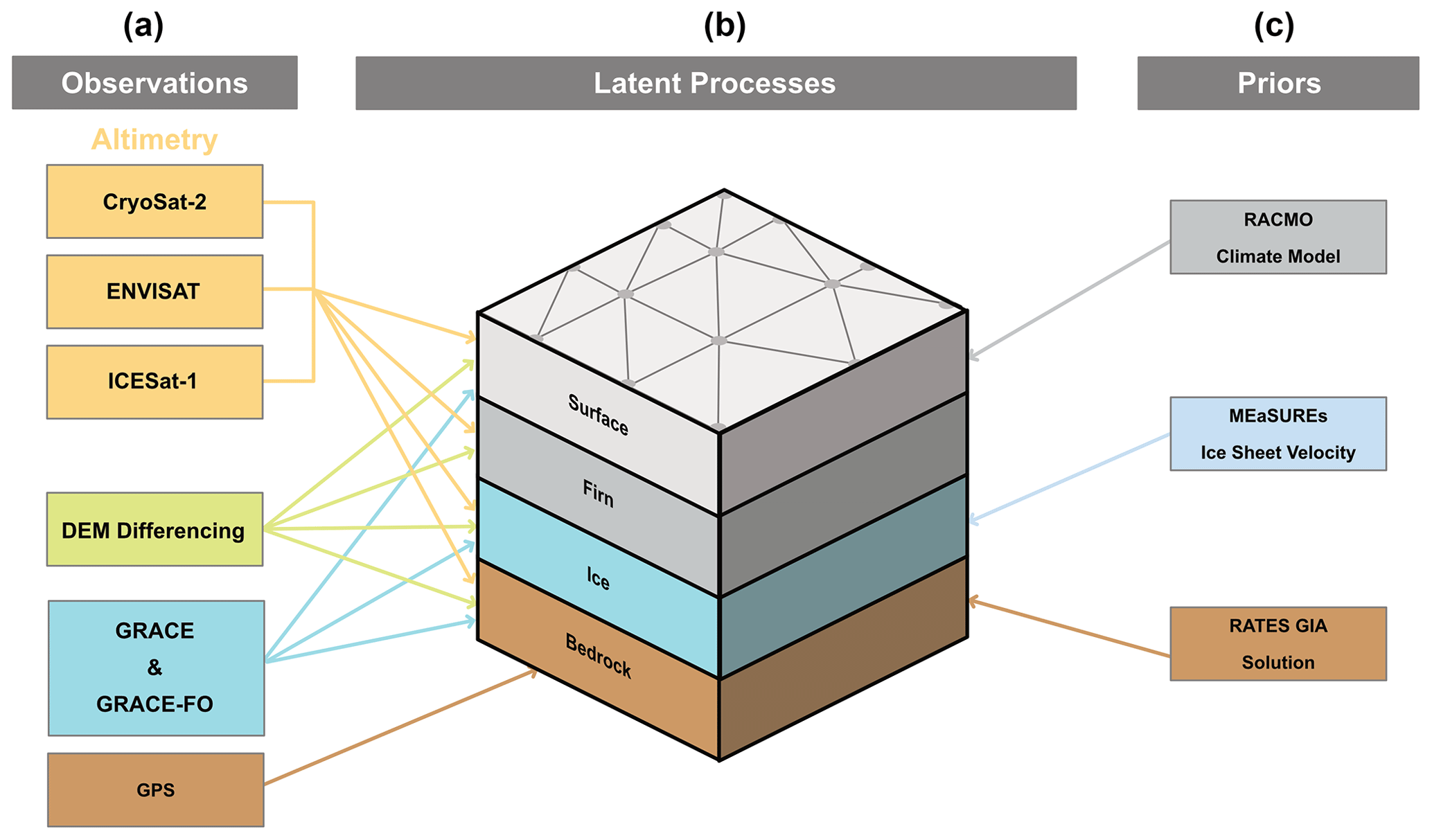
Figure 2Conceptual overview of the BHM framework. Panel (a) shows the observations used in the framework, with arrows linking the observations to the latent processes they observe. Panel (b) outlines the ice sheet processes being solved for in the BHM using the FEMs (grey triangles and circular mesh nodes). Panel (c) shows the prior information used to aid source separation of the observations into the latent processes.
The large-scale ice sheet solution of Martín-Español (2016) produced a data-driven temporally invariant estimate of vertical land uplift rates due to GIA. We use this GIA solution as an informative prior (i.e. as the prior mean field) on the GIA latent process in this model, additionally constrained by the GPS observations in Martín-Español (2016). This means we are not solving for a new GIA solution but instead enforcing a hard constraint on the latent process and following the iterative solution approach of Martín-Español (2016).
Recently, satellite remote sensing observations of ice sheet behaviour have shown complex spatio-temporal evolution patterns in ice dynamics, such as Pine Island Glacier (Bamber and Dawson, 2020). As a result, the linear and quadratic functions used to describe the temporal evolution of ice dynamics in previous studies using this framework (Martín-Español et al., 2016) may not adequately represent the complexity of the dynamic signal over longer (multi-decadal) time series. In the BHM we therefore allow for a less restrictive temporal evolution of mass change due to ice dynamics. Specifically, we use a first-order autoregressive (AR(1)) process to describe the temporal evolution of ice dynamics. We fix the autoregression coefficient to 0.8, which implies a strong temporal dependence in time and consistent with marine ice sheet models operating at the same temporal resolution (Robel et al., 2018). Model analysis of response times of glaciers draining into West Antarctica to instantaneous forcing range from 6.4 years (Ferrigno Ice Stream) to 18.3 years (Thwaites) (Williams et al., 2012), equating to AR(1) coefficients of 0.73–0.90 (Storch and Zwiers, 1999). Therefore, the selection of 0.8 for the AR(1) coefficient provides an appropriate prior description of the smoothness of the process, whilst allowing for sufficient flexibility to capture changes that may occur in response to variations in ocean forcing. This new latent process behaviour also allows the framework far greater flexibility over longer timescales, future-proofing the approach for multi-decadal studies.
3.2.1 MEaSUREs V2 velocity product
The velocity field used to help inform the spatial variance in the ice dynamics process (Schoen et al., 2015) has also been updated to the MEaSUREs V2 composite velocity product (Mouginot et al., 2012; Rignot et al., 2011c, 2017). The 99.6 % Antarctic Ice Sheet coverage in the updated product (Mouginot et al., 2017) precludes the need for balance velocities to be used to fill missing data regions. This is particularly beneficial in the mountainous interior of the southern AP, where coverage from InSAR data was previously limited.
3.2.2 RACMO SMB product
To determine the spatio-temporal length scales of surface mass balance over the mountainous terrain in the AP, we use the RACMO2.3p2 5.5 km model. Its higher resolution improves its capability to resolve large SMB gradients from west to east over the northern AP, in addition to the narrow outlet glaciers feeding into the ice shelves, when compared to the ice-sheet-scale ∼27 km resolution model (van Wessem et al., 2016). We use RACMO 5.5 km SMB anomalies with respect to the 1979–2002 baseline for drainage sectors incorporated in the AP (Fig. 1) as outlined in the most recent Ice Sheet Mass Balance Inter-comparison Exercise (IMBIE) assessment (Shepherd et al., 2018). For sectors outside the AP, the ice-sheet-wide RACMO 27 km 2.3p2 model is used. As only spatio-temporal spectral properties are determined from the regional climate models (RCMs), the use of models at two different resolutions does not bias or create discontinuity in our prior for the surface latent process field. This is an advantage of our approach: by not using the raw model output, we are able to incorporate prior information for each region without introducing discontinuities.
Our results indicate that over the 17-year period of our study (2003–2019), the AP has experienced a mean mass imbalance of Gt yr−1, with the largest rates of mass changes occurring between 2008 and 2015 (Fig. 3 and Table 2). In the last 3 years of our study, reductions in mass imbalance are seen across all basins, primarily because of an extreme snowfall event in 2016. The underlying driver of region-wide mass imbalance is dynamic mass losses across the sector ( Gt yr−1), with no emergent trend in the surface processes present over the study period. As can be seen from Fig. 3, however, the large inter-annual variability in mass balance is a result of the superposition of the SMB changes in the total signal, which are large enough to temporarily change the mass balance state of the whole sector for an individual year (e.g. 2016 and 2017). Therefore, the use of time average mean mass balance estimates over short temporal baselines for this sector can be misleading.
Table 2Mean mass trends for the 2003–2019 period of the study and over various epochs for the AP region and individual basins (see Fig. 1 for drainage basin and region definitions; Rignot et al., 2011a, 2013) All uncertainty states as 1σ.
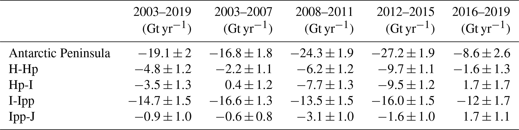
At the individual drainage basin scale (Fig. 4), the same spatio-temporal pattern of process behaviour is evident across the northern AP (basin I-Ipp), West Palmer Land region (Hp-I), and Abbot sector (H-Hp), with ice dynamics in the northern AP region forming a larger proportion of the overall total imbalance in comparison to the other AP basins (Fig. 4). In contrast, the eastern portion of the southern AP (Ipp-J) has remained in a steady state of dynamic balance for the entirety of the study period, with mass trend fluctuations driven wholly by SMB.
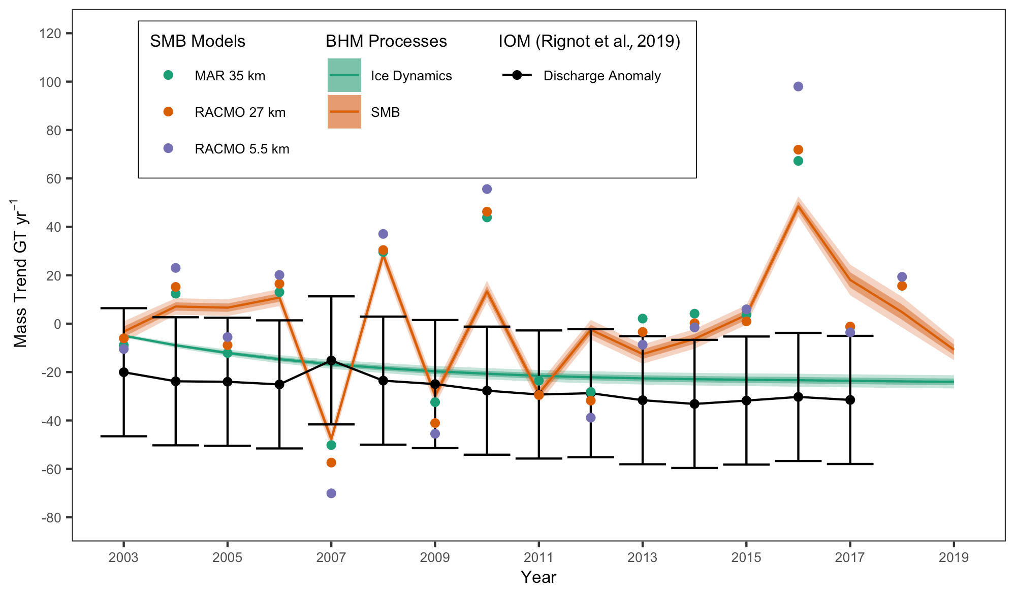
Figure 3SMB and ice dynamic mass trends for the AP region (line plots, with shaded ribbons representing 1σ and 2σ uncertainties). Scatter points represent RCM mass anomalies with respect to a 1979–2002 baseline (Agosta et al., 2019; van Wessem et al., 2016, 2018), and the black line represents the annual ice discharge anomaly with respect to a 1979–2002 baseline value, with the 1σ uncertainty on the discharge represented by the crossbars as stated in Rignot et al. (2019). See Sect. S1 for methodologies used for dataset intercomparison.

Figure 4BHM mass trends and constituent processes for each individual drainage basin in the study region (Rignot et al., 2011b, 2013); see Fig. 1 for drainage basin locations. Dark and light ribbons represent the 1σ and 2σ uncertainty of mass trends, respectively.
4.1 Ice dynamics
The temporal pattern of ice dynamic mass changes is similar across the northern AP (I-Ipp), West Palmer Land (Hp-I), and the Abbot sector (H-Hp) (Fig. 4). Between 2003 and 2010 there is an acceleration in mass loss due to ice dynamics, whereas in the last decade the rate of acceleration either slows or reaches a new state of disequilibrium. As can be seen from Fig. 3, for the AP as a whole, comparisons of the BHM ice dynamics mass trend estimated with the ice discharge component of an input–output method (IOM) approach (Rignot et al., 2019) show a similar temporal evolution, albeit with slight negative bias in discharge anomaly with respect to the BHM trends. The congruent nature of the ice dynamics response for basins draining into the Bellingshausen Sea sector implies an external oceanic forcing mechanism is the likely driver. This is supported by observations showing rapid ice shelf thinning and therefore reduced buttressing capability to the grounded ice sheet since 1994, with the Venable Ice Shelf in the Bellingshausen Sea sector showing some of the largest rates of thinning across Antarctica (Paolo et al., 2015). In contrast the eastern side of the AP (basin Ipp-J), draining into the Weddell Sea shows no change in ice dynamics signal according to our BHM estimates. This is consistent with observed deep ocean water temperatures of several degrees above the seawater freezing point in the Bellingshausen Sea sector, as opposed to the Weddell Sea where they have stayed near freezing point (Adusumilli et al., 2020). Our ice dynamic trends reflect these contrasting patterns in ocean forcing between the east and west sides of the AP.
In the northern AP, the temporal evolution of ice dynamic imbalance for the period 2001–2010 is consistent with the rapid acceleration and increases in ice discharge of outlet glaciers after the collapse of the Larsen A and B ice shelves in 1998 and 2002, respectively (Scambos et al., 2014), and subsequent deceleration in mass loss (Rott et al., 2018). The Hektoria and Green glaciers draining into the Larsen B embayment show some of the largest thinning rates across the AP, with an estimated m yr−1 of the total elevation change signal in 2010 near the grounding line attributed to ice dynamics.
In the West Palmer Land drainage basin (Hp-I), ice dynamic mass loss is concentrated in outlet glaciers draining the English coast into the George VI ice shelf, the Nitikin Glacier, and the Berg and Thompson ice streams, in addition to the dynamic thinning of glaciers draining into the Wordie ice shelf after its collapse in 1990s (Fig. 5). Towards the interior of the drainage basin, there is an emergence of a small ice dynamic thickening signal, which is notable due to the slow ice flow in this region. Elevation changes from satellite altimetry have shown the same pattern of thickening over the higher-elevation regions of this basin since 2003 (Schröder et al., 2019; Smith et al., 2020). Any long-term temporal trend in ice thickening due to a sustained increase in precipitation may be partially misattributed as an ice dynamic signal by the framework, due to it being a temporally smooth and sustained increase in mass over time. Over the course of the 20th century there have been sustained large increases in precipitation over the AP, providing an explanation for this misrepresentation (Medley and Thomas, 2019; Wang et al., 2017).
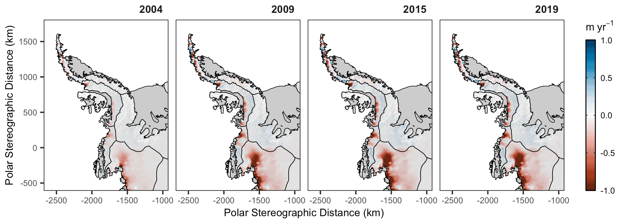
Figure 5Temporal evolution of height changes due to ice dynamics for 4 years over the course of the 17-year study period. The colour scale is saturated at end points for plot clarity. The basin outlines and grounding line are overlain in black (Rignot et al., 2011b, 2013). Dark grey regions represent ice shelves (Depoorter et al., 2013). Data are overlain on the hill shade of the REMA DEM (Howat et al., 2019).
To the west of the AP along the Bellingshausen coastline, the Abbot sector has experienced an increase in ice dynamic mass loss over the period of the study, driven primarily by the Fox, Ferrigno, Wiesnet, and Williams ice streams (Fig. 1a). The ice shelves buttressing these ice streams have seen nearly a one-fifth reduction in ice thickness since 1994 (Paolo et al., 2015), which supports the dynamic thinning behaviour seen in the BHM output. This is in direct contrast to the rest of the glaciers in this basin draining into the Abbot Ice Shelf, which has experienced no dynamic induced thinning over the course of the last 2 decades. This corroborates with other mass budget studies (Chuter et al., 2017) and the absence of grounding line retreat over several decades (Christie et al., 2016).
4.2 Surface processes
Changes in surface processes are the major drivers of inter-annual variability in mass balance, with the total contribution to the mass trend ranging between Gt yr−1 in 2007 and 48.5±2.1 Gt yr−1 in 2016 (Fig. 3). The largest positive trends in surface processes, in 2016 and 2017, coincide with the extreme El Niño–Southern Oscillation event, which resulted in increased precipitation, most noticeably across the western AP (Bodart and Bingham, 2019). This temporarily restored the total mass trend of the sector to a state of positive balance after sustained negative surface process mass trends between 2010 and 2015. Over the whole AP sector, our trends in surface mass on the whole follow the inter-annual variations in the output of three RCMs (Fig. 3), with the BHM solution generally showing a weaker signal compared to the RCM output for some years (e.g. 2010 and 2016).
In 2016 and 2017, the BHM allocates the majority of SMB increase in the West Palmer Land region of the southern AP (basin Hp-I), with minimal SMB gains observed on the eastern side (Fig. 6). This is in good agreement with the output from the RACMO 2.3p2 5.5 km climate model for 2016, although the RCM output reports much greater and widespread height change. Significant surface-process-driven height changes are also partially resolved in the northern AP, although without the same clear separation in signal characteristics along its mountain spine. This is most likely due to the paucity of altimetry observations available in this region, despite the increase in observational coverage provided by the CryoSat-2 Swath data, inhibiting localization of the smooth signal representation that would be shown by GRACE. Additionally, the very small width of the region (largely less than 100 km in width) limits the ability of GRACE to observe mass changes in this part of the AP.
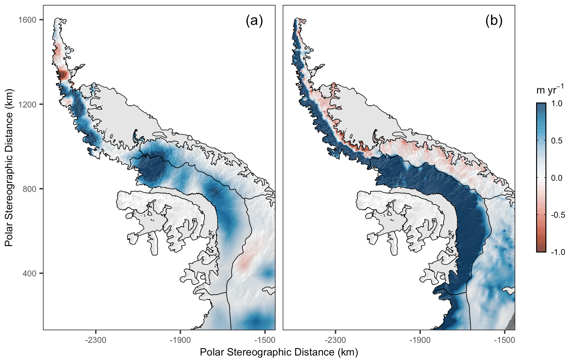
Figure 6Changes in ice sheet elevation due to SMB from the (a) BHM and (b) RACMO2.3p2 5.5 km RCM (van Wessem et al., 2016) for the year 2016. The colour scale is saturated at end points for clarity. The basin outlines and grounding line are overlain in black (Rignot et al., 2011b, 2013). Dark grey regions represent ice shelves (Depoorter et al., 2013). Data are overlain on the hill shade of the REMA DEM (Howat et al., 2019).
At the individual basin scale, Fig. 7 shows that the BHM surface process output generally follows the temporal variability in the suite of RCMs used for comparison across all basins. This is particularly evident between 2007 and 2011, where the BHM posterior replicates the large positive to negative inter-annual variations in surface processes that are present in all the RCM solutions, albeit with a wide variation in absolute magnitude between both the BHM and each regional RCM. This is expected due to the varying spatial resolutions of the climate models, which govern their capability to resolve small-scale orographically driven processes, in addition to the BHM posterior being driven by observations rather than a physical model of climate processes. The mismatch of magnitude is most prominent in the Hp-I basin, where the RCM output in large anomaly years appears to be consistently either more positive or negative than that of the BHM output. The basin-aggregated SMB posterior magnitudes are more certain than the marginal (spatial pointwise) posterior standard deviations, due in part to the relative smoothness of the process and the large spatial resolution of some of the observations. An example of the posterior standard deviations associated with our predictions for SMB and ice dynamics for the year 2010 is shown in Fig. S1 and in dataset S2.
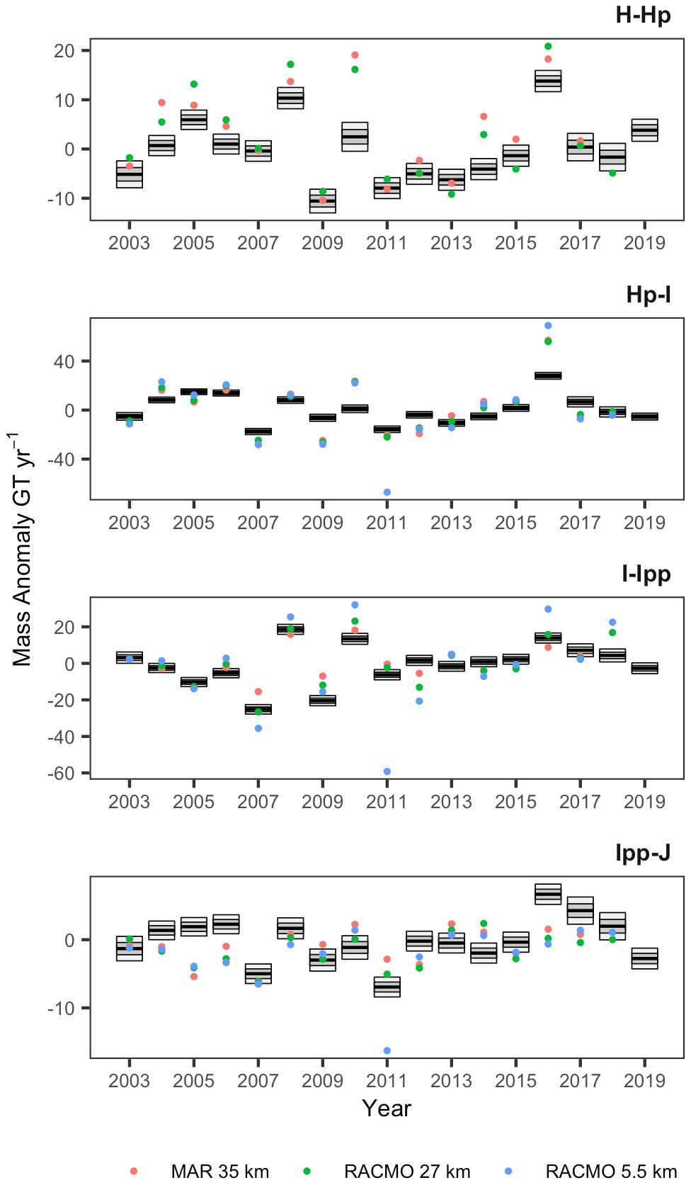
Figure 7Comparison of BHM SMB posterior mass trends with RCM output for each year of the study, at the individual basin scale. Black lines represent BHM posterior mean, with dark and light grey boxes representing the 1σ and 2σ uncertainty, respectively, on the latent process. Points represent the output from different RCMs (Agosta et al., 2019; van Wessem et al., 2016, 2018). Note that spatial coverage of the RACMO2.3p2 5.5 km model does encompass the full area of basin H-Hp (Abbot sector) and is therefore excluded from analysis in this region. Methodology used for dataset comparison is outlined in Sect. S1.
Our annual mass trend time series for the AP sector shows good general agreement with a variety of time-mean mass balance estimates from different approaches in addition to the IMBIE assessment (Shepherd et al., 2018) (Fig. 8). Our time-mean results are in best agreement with altimetry- and gravimetry-based approaches, though they tend to give more positive mass balance trends than those previously calculated using IOM approaches. This can be partially explained by the fact that our BHM solution is driven primarily by gravimetry and altimetry observations, so it would be expected that the results would be in better general agreement with these approaches. We also find good overall agreement between our time series and IMBIE for the period 2003–2017 (Shepherd et al., 2018) in terms of the temporal mass trend evolution, showing large variations in mass between 2006 and 2010 and the extreme El Niño-driven precipitation event in 2016. On average, our BHM estimate of mass imbalance is slightly more positive than that of the IMBIE time series, which we attribute to the fact that the latter approach gives equal weighting to estimates from mass budget techniques (which tend to suggest more negative mass balance) in the combined time series. Between 2003 and 2010, the IMBIE study reports negative trends from mass budget approaches that are more than double those calculated using either altimetry or gravimetry, which would propagate into a more negative combined trend (Shepherd et al., 2018). However, the general overall agreement between the two studies demonstrates the value that multiple independent combination approaches can have in improving confidence in mass balance assessments for this challenging region.
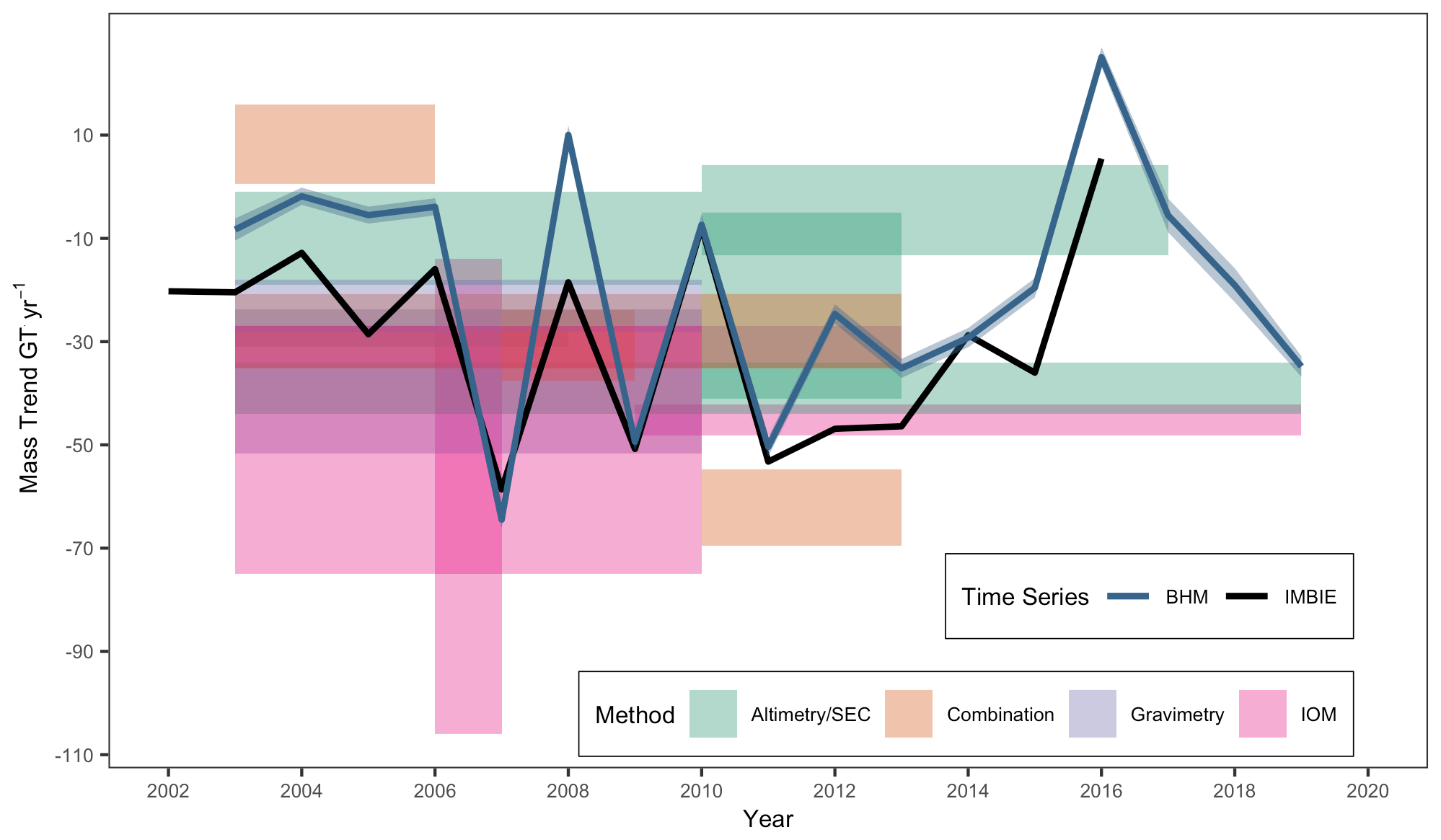
Figure 8Comparison of total mass trends for the AP from the BHM (blue line, with 1σ uncertainty ribbon) with time-averaged epoch studies for the same sector (colour shaded boxes – see Table S1 for list of studies) and the annual mass trends from the IMBIE exercise (Shepherd et al., 2018). Details of the processing for the comparison datasets can be found in Sect. S1.
When looking at the individual drivers of mass change for the sector as a whole, IOM studies show that the AP has exhibited increases in ice discharge over the last 2 decades, with an estimated increase in discharge of 14 Gt yr−1 between 2003 and 2017 (Rignot et al., 2019) and 7±6 Gt yr−1 between 2008 and 2015 (Gardner et al., 2018). Our ice dynamics solution shows a similar magnitude of ice mass loss over the same period, with an estimated 19.1 Gt yr−1 increase between 2003 and 2017 and an estimated 4.8 Gt yr−1 increase between 2008 and 2015. Whilst our rates of change in discharge are generally in agreement with IOM studies, there are differences of over 100 Gt yr−1 in the absolute annual ice discharge for contemporaneous time periods over the AP basin (Gardner et al., 2018; Rignot et al., 2019). As a result, calculation of total mass balance using an IOM approach is highly conditional on the choice of baseline. Additionally, it highlights the importance for continuing improvements in the determination of ice thickness and ice velocity at the grounding line. An advantage of the BHM approach is that it does not require assumptions regarding the balance state of the ice sheet, therefore negating the potential for biases and uncertainties that can occur in the IOM approach.
At the basin scale, reconciling mass balance estimates over the western part of the southern AP (basin Hp-I) for the last 2 decades has been challenging. For example, two mass balance studies utilizing CryoSat-2 radar altimetry and covering the same period (albeit with differing volume-to-mass conversion philosophies) do not agree within error. The first, using an ice dynamic imbalance mask conversion approach (McMillan et al., 2014), estimated a mass loss of 11±11 Gt yr−1, while the second, using the output of regional climate models, estimated a mass loss of 34±12 Gt yr−1 (Wouters et al., 2015). For the same 2011–2014 period, our study gives a total mass loss of 13.8±1.2 Gt yr−1, consisting of an ice dynamics contribution of Gt yr−1 (38 %) and a surface process contribution of Gt yr−1 (62 %). This time period coincides with the consistent negative BHM surface process trend between 2010 and 2015, as shown in Fig. 9a, and is in agreement with the negative mass anomalies from RCMs for the same time period. The presence of an ice dynamic thinning signal on the southern sections of the West Palmer Land basin in our solution is consistent with the largest rates of basal-melt-driven ice shelf thinning over the George VI ice shelf of 7±2 m yr−1 for the period 1994–2016 (Adusumilli et al., 2018) (Fig. S2a), supporting a joint ice sheet mass loss forcing mechanism for this period of time. Our results suggest that surface processes were the largest contributor to total mass imbalance between 2011 and 2014, as opposed to ice dynamics. Therefore, it is likely that the use of a dynamic imbalance mask underestimates the ice dynamics contribution (as no areas of this basin were defined a priori to be in an ice dynamics imbalance state), whereas potential biases in the SMB and firn model correction may have underestimated the surface process contribution. This challenge is demonstrated when we compare our time series with other studies over the 17-year period (Fig. 9b), for which there is large divergence between time mean mass balance studies since 2010. Whilst our time series is situated in the middle of the spread of results, different altimetry studies disagree on the sign of mass balance for overlapping periods. This is due in combination to outlined methodological challenges using altimetry observations and to time mean studies not being able to represent the large inter-annual surface-process-driven variability we see in our mass trend after 2010.
The separation of ocean and ice mass change signals in gravimetry approaches can greatly affect the resultant mass anomaly time series, in particular for the AP and Hp-I basin (Bodart and Bingham, 2019). In terms of basin leakage impacts, other combination approaches with altimetry and gravimetry have shown that the inclusion of the former reduces the correlation in mass change signal between neighbouring basins compared to using gravimetry alone (Sasgen et al., 2019). Considering the Hp-I basin is surrounded by large mass losses from the Abbot and Amundsen Sea sector to the south and west, in addition to mass losses over the northern AP, the leakage of signals from neighbouring basins is likely to impact gravimetry mass changes in this locality. Additionally, the Sasgen et al. (2019) combination study noted the ability for altimetry to observe small spatial mass gain signals due to increased snowfall, which cannot be resolved by gravimetry alone. As we see in our results for 2016 for this basin (Fig. 6), its susceptibility to large variations in mass from extreme snowfall events may limit agreement between the two observational approaches. Agreement between the two approaches is also possible as the result of a cancellation of errors.
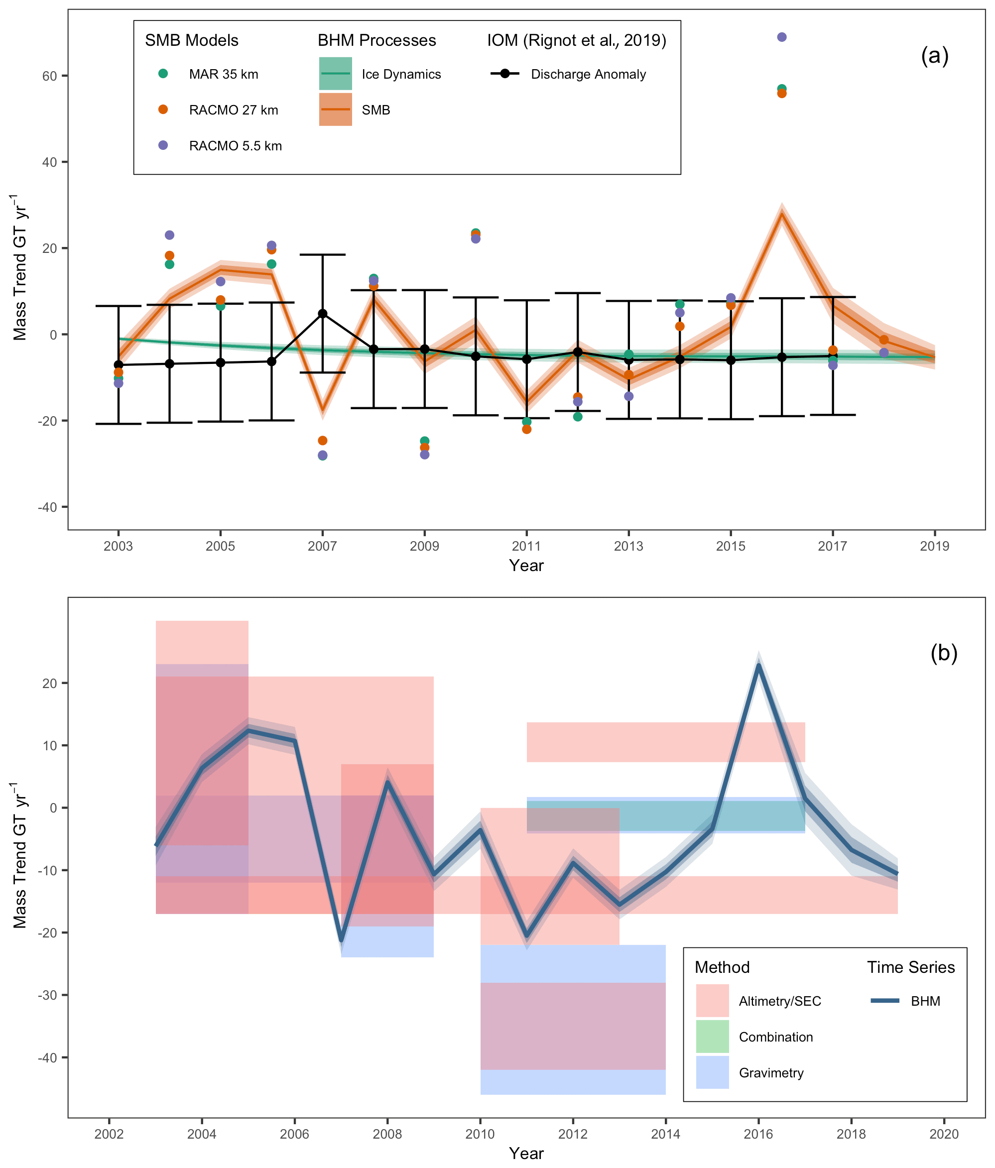
Figure 9(a) Surface processes and ice dynamics mass trends for the Hp-I drainage basin (West Palmer Land and English Coast region) line plots, with shaded ribbons representing 1σ and 2σ uncertainties on the process posterior from the BHM. Scatter points represent RCM mass anomalies with respect to a 1979–2002 baseline (Agosta et al., 2019; van Wessem et al., 2016, 2018), and the grey line represents the annual ice discharge anomaly with respect to a 1979–2002 baseline value, with one 1σ uncertainty on the discharge represented by the crossbars (Rignot et al., 2019). (b) Comparison of total mass trends for basin Hp-I from the BHM (blue line, with 1σ uncertainty ribbon) with time-averaged epoch studies for the same sector (colour shaded boxes – see Table S2 for list of studies). Details of the processing for the comparison datasets can be found in Sect. S1.
Mass budget studies of this basin suggest that the magnitude of ice discharge has been relatively constant, with increases in ice discharge of up to 15 km3 yr−1 over 3 decades (Gardner et al., 2018; Hogg et al., 2017). This small increase is reflected in our results, which show an acceleration of ice dynamic mass losses up until 2008, with little change thereafter. This temporal evolution is supported by Gardner et al. (2018), who find an increase of 2±3 Gt yr−1 in ice discharge between 2008 and 2015, in addition to the agreement of our results with ice discharge anomalies from Rignot et al. (2019) as seen in Fig. 9a. An analysis of velocity change for 2005–2011 to 2011–2017 (Sect. S2 and Fig. S2b) shows minimal changes across the basin, with highly localized accelerations near the grounding line of some individual outlet glaciers. Whilst this would suggest that mass losses due to dynamic imbalance should increase, the thinning of these outlet glaciers could be offsetting expected increases in discharge. These independent assessments support the magnitude of ice dynamic mass losses we see from the BHM approach in this basin. It should be noted that, unlike in our study, the Wordie Ice Shelf is not included in these IOM basin definitions, and our ice dynamic trends may, therefore, show a slight underestimation for the basin. The slight ice dynamic thickening signal we see in our solution in the interior of the basin as result of a long-term snowfall accumulation trend may, in part, be misrepresented as an ice dynamic process and be partially responsible for this discrepancy.
The previous implementation of the BHM framework over this region showed total mass losses between 2010 and 2013 of 39±5 Gt yr−1, primarily driven by ice dynamics (Martín-Español et al., 2016). Whilst the basins used in that study included the eastern side of the southern AP, minimal mass fluctuations in this region are not expected to significantly compromise comparisons with our study. We believe the discrepancy between our study and the previous implementation is due in part to the linear temporal ice dynamics constraint applied in previous iterations of the framework. The use of a linear model would not be able to capture accelerations in dynamic thinning in the early 2000s followed by a slowdown in ice discharge imbalance after 2008 that we, and other independent approaches (Gardner et al., 2018; Rignot et al., 2019), have detected in this region. This demonstrates the new ice dynamics process implementation's suitability for multi-decadal studies.
Another benefit of our approach can be seen in 2017 and 2018, when gravimetry observations are not available due to the gap in coverage between the GRACE and GRACE-FO missions. Gravimetry is a key observation in our framework as it is the only available direct observation of mass change and, when combined with altimetry, is critical in aiding source separation of driving processes. However, despite the BHM being solely driven by CryoSat-2 altimetry data during this period, the BHM ice dynamics posterior trend over this period retains its smooth variation. Surface process mass trends also remain in good general agreement with temporal variations in RCM output (Figs. 3 and 7), albeit with slightly larger uncertainty bounds. The ability to successfully bridge this gap is a key practical demonstration of one of the major benefits of our BHM approach for the first time. It provides confidence that our combination approach can handle future potential unforeseen gaps or other changes in either the altimetry or gravimetry observation record, maintaining the long-term continuous time series required to ascertain the driving forces of ice sheet mass balance.
Despite the considerable progress made in this study, we can identify several limitations and potential future improvements with our implementation of a BHM framework. First, the validity of the BHM approach in mass balance studies largely hinges on our assumptions about the underlying latent processes and priors being representative of the geophysical processes being solved. In previous implementations of the BHM framework, assuming a linear or quadratic temporal variation in ice dynamics was generally adequate due to the short length of the time series (<10 years). The change in implementation to an AR(1) process with drift for ice dynamics in this study addresses a potential issue with extending the time series over multiple decades. However, the high coefficient used on the AR(1) process means the underlying assumption remains that the process is temporally smooth, similar to what we observe in the output of ice sheet models. Therefore, any sudden changes in ice dynamics (sub-annual to annual), such as resulting from sudden ice shelf collapse, may not be represented immediately in this latent process and may take several years to be appropriately attributed. This modelling assumption is apparent in the temporal smoothness properties of our ice dynamics mass trends in comparison with variability seen in the ice discharge component of mass budget approaches (Figs. 3 and 9a) (Rignot et al., 2019). Future priors can address this by taking advantage of recent ice-sheet-wide repeat velocity measurements (Fahnestock et al., 2015) and allowing for the implementation of a spatio-temporal prior linking ice dynamics to velocity.
Second, despite the increases in observation coverage and mesh density, challenges remain separating latent processes in the northernmost sectors of the AP. This is in part due to the basin's latitudinal position reducing the spatial density of coverage available from satellite altimetry, as well as its small spatial scale relative to the native resolution of GRACE. The incorporation of dDEM data into the framework, although spatially limited in its coverage, alleviates this issue somewhat and demonstrates the potential for improving mass change estimates in the future, as exemplified over the Hektoria and Green glaciers. Additionally, it should be noted that the dDEM data pre-processing exclusion of elevation trends in regions of grounding line migration may introduce a small bias with the GRACE data where large mass change signals occur in this vicinity. Whilst this bias is reduced compared to conventional altimetry techniques alone, it is still potentially present. The recent launch of ICESat-2, in addition to more widespread repeat dDEM data from the REMA project, should greatly enhance our ability to monitor the mass balance of this key region into the next decade. The spatial length scale of the processes we solve for is limited by the resolution of the prior information used in the model. Therefore, in regions as heterogenous as the northern AP, improved-resolution climate models and statistical downscaling approaches (Noël et al., 2016) will aid small-spatial-scale process separation. An additional future model development could be the introduction of a barrier model to enforce spatial independence in regions which, whilst in close spatial proximity, are largely spatio-temporally independent. This would be useful to capture, for example, the differing SMB characteristics between the east and west sides of the Antarctic Peninsula mountain range.
Third, many of the observations used in the framework are from multi-year trends, necessitated by the satellite repeat revisit time and to ensure robust trend estimation. However, this can, in effect, apply a low-pass filter to the observations, which may reduce inter-annual changes in SMB seen by the framework. Whilst the inter-annual patterns in surface process mass trend variation are similar between the model outputs and geophysical models (Fig. 7), the BHM posterior field appears to have a reduced amplitude compared to that of the geophysical models in some basins (e.g. Basin Hp-I), which would be indicative of the observations being used. This caveat should therefore be considered in the interpretation of these fields. Whilst higher-temporal-resolution sensors will allow multi-annual trend estimation, it still present a challenge when combining diverse observations with differing spatio-temporal observation characteristics (Shepherd et al., 2018).
Finally, recent advances in our understanding of the much more rapid than previously assumed (decadal length scales) viscous response of the mantle to changes in ice mass loading for certain sectors of Antarctica (Barletta et al., 2018; Nield et al., 2014) presents a future opportunity for the framework. Incorporation of a temporally evolving latent process for GIA, coupled with GPS observations over the whole study period, could provide the opportunity for a temporally varying data-driven inverse GIA field. Although GIA is not a major contributor to mass changes in the AP, and therefore not a significant source of uncertainty in this study, such a solution would provide insights into the solid Earth response and its potential impact on both ice sheet stability (Larour et al., 2019) and variations in local sea level change around the globe.
In this study we estimate the mass evolution of the AP, in addition to its driving constituent processes, at an annual resolution for the period 2003–2019 using a BHM framework. Our results indicate that the sector experienced an overall mean mass loss of 19.1±2 Gt yr−1 in this time, driven by an acceleration in ice dynamic imbalance over the first decade of this century and continuing at a lower rate thereafter until present. In contrast, no trends in surface processes are evident over the period of the study, although at annual timescales, they still govern the mass balance state of the region. Our solution provides good agreement with a range of RCM SMB estimates at both the sector and individual basin scales, reflecting the main inter-annual variability of the surface process mass trends. Additionally, our ice dynamic mass losses support the general trends in ice discharge seen in independent mass budget studies. We find in the West Palmer Land region (Hp-I) our solution indicates that surface processes are a more likely driver of the large mass losses seen between 2011 and 2014, highlighting the challenges and improvements in the necessary assumptions that need to be made in the volume-to-mass conversion when using conventional altimetry approaches, particularly when multiple driving processes are occurring in spatially coincident locations. Additionally, addressing the GRACE/GRACE-FO gap highlights the benefit of a combination approach in ensuring the continuation of high-resolution mass change time series over the course of multiple decades, which is crucial for attributing the role of differing external forcing in driving ice sheet mass change. The enhanced BHM framework presented in this study, in combination with emerging state-of-the-art high-resolution Earth observations such as WorldView and ICESat-2, lays the foundation for the extension of the approach over the next decade.
Finite element meshes used in this study were constructed using the R-INLA software package (https://www.r-inla.org, last access: 11 August 2020; Rue et al., 2009, https://doi.org/10.1111/j.1467-9868.2008.00700.x). Bayesian inference was undertaken using the freely available MVST(V2.0) R package developed by AZM & SJC (https://github.com/andrewzm/MVST, last access: 1 November 2018; Zammit-Mangion et al., 2015a, https://doi.org/10.3189/2015AoG70A021; Zammit-Mangion et al., 2015b, https://doi.org/10.1002/env.2323).
The Bayesian hierarchical model annual mass trends, including constituent processes, are provided in supplementary Dataset S1. The spatial fields used for the visualizations in this paper are provided in Dataset S2. CryoSat-2 Swath data used in this study were processed by CryoTEMPO-EOLIS (https://www.cryotempo-eolis.org, last access: 10 December 2020, ESA, 2020) and distributed by ESA (https://science-pds.cryosat.esa.int/, last access: 10 December 2020; Gourmelen et al., 2018, https://doi.org/10.1016/j.asr.2017.11.014). Ice shelf net mass balance data from Adusumilli et al. (2018) are available from https://sealevel.nasa.gov/data/dataset/?identifier=SLCP_AP_iceshelf_mass_balance_1 (last access: 15 April 2021; Adusumilli et al., 2018, https://doi.org/10.1002/2017GL076652). The MEaSUREs annual velocity maps used are available at https://doi.org/10.5067/9T4EPQXTJYW9.
The supplement related to this article is available online at: https://doi.org/10.5194/tc-16-1349-2022-supplement.
SJC conceptualized the study, undertook the analyses, and wrote the manuscript. AZM developed the original MVST R software package and assisted SJC in implementation of model improvements. GD provided significant discussions on altimetry processing and swath data analysis. JR advised on the statistical inference framework and the methodology. JLB assisted in methodological discussions and the analysis of results. All authors discussed the results and provided comments on the manuscript.
The contact author has declared that neither they nor their co-authors have any competing interests.
Publisher’s note: Copernicus Publications remains neutral with regard to jurisdictional claims in published maps and institutional affiliations.
We would like to thank the two anonymous reviewers for their valuable comments and improvements to the manuscript. We would like to thank Ted Scambos for providing the dDEM and ICESat data used in this study over the northern AP. We also acknowledge Melchior Van Wessem for providing the RACMO2.3p2 SMB and surface density products used in this study.
This work was supported by European Research Council (ERC) under the European Union's Horizon 2020 research and innovation programme under grant no. 694188 (GlobalMass). Jonathan Bamber was also funded by the German Federal Ministry of Education and Research (BMBF) international future AI lab “AI4EO – Artificial Intelligence for Earth Observation” (grant no. 01DD20001). Andrew Zammit-Mangion's research was supported by ARC Discovery Early Career Research Award (DECRA) DE180100203 and by ARCRIEAS grant no. SR200100005, Securing Antarctica's Environmental Future. Geoffrey Dawson was supported by the UK Natural Environment Research Council (NERC) grant no. NE/N011511/1.
This paper was edited by Stef Lhermitte and reviewed by two anonymous referees.
Adusumilli, S., Fricker, H. A., Siegfried, M. R., Padman, L., Paolo, F. S., and Ligtenberg, S. R. M.: Variable Basal Melt Rates of Antarctic Peninsula Ice Shelves, 1994–2016, Geophys. Res. Lett., 45, 4086–4095, https://doi.org/10.1002/2017GL076652, 2018 (data available at: https://sealevel.nasa.gov/data/dataset/?identifier=SLCP_AP_iceshelf_mass_balance_1 (last access: 15 April 2021).
Adusumilli, S., Fricker, H. A., Medley, B., Padman, L., and Siegfried, M. R.: Interannual variations in meltwater input to the Southern Ocean from Antarctic ice shelves, Nat. Geosci., 13, 616–620, https://doi.org/10.1038/s41561-020-0616-z, 2020.
Agosta, C., Amory, C., Kittel, C., Orsi, A., Favier, V., Gallée, H., van den Broeke, M. R., Lenaerts, J. T. M., van Wessem, J. M., van de Berg, W. J., and Fettweis, X.: Estimation of the Antarctic surface mass balance using the regional climate model MAR (1979–2015) and identification of dominant processes, The Cryosphere, 13, 281–296, https://doi.org/10.5194/tc-13-281-2019, 2019.
Bamber, J. L. and Dawson, G. J.: Complex evolving patterns of mass loss from Antarctica's largest glacier, Nat. Geosci., 13, 127–131, https://doi.org/10.1038/s41561-019-0527-z, 2020.
Bamber, J. L., Westaway, R. M., Marzeion, B., and Wouters, B.: The land ice contribution to sea level during the satellite era, Environ. Res. Lett., 13, 063008, https://doi.org/10.1088/1748-9326/aac2f0, 2018.
Barletta, V. R., Bevis, M., Smith, B. E., Wilson, T., Brown, A., Bordoni, A., Willis, M., Khan, S. A., Rovira-Navarro, M., Dalziel, I., Smalley, R., Kendrick, E., Konfal, S., Caccamise, D. J., Aster, R. C., Nyblade, A., and Wiens, D. A.: Observed rapid bedrock uplift in amundsen sea embayment promotes ice-sheet stability, Science, 360, 1335–1339, https://doi.org/10.1126/science.aao1447, 2018.
Bodart, J. A. and Bingham, R. J.: The Impact of the Extreme 2015–2016 El Niño on the Mass Balance of the Antarctic Ice Sheet, Geophys. Res. Lett., 46, 13862–13871, https://doi.org/10.1029/2019GL084466, 2019.
Borsa, A. A., Moholdt, G., Fricker, H. A., and Brunt, K. M.: A range correction for ICESat and its potential impact on ice-sheet mass balance studies, The Cryosphere, 8, 345–357, https://doi.org/10.5194/tc-8-345-2014, 2014.
Christie, F. D. W., Bingham, R. G., Gourmelen, N., Tett, S. F. B., and Muto, A.: Four-decade record of pervasive grounding line retreat along the Bellingshausen margin of West Antarctica, Geophys. Res. Lett., 43, 5741–5749, https://doi.org/10.1002/2016GL068972, 2016.
Chuter, S. J., Martín-Español, A., Wouters, B., and Bamber, J. L.: Mass balance reassessment of glaciers draining into the Abbot and Getz Ice Shelves of West Antarctica, Geophys. Res. Lett., 44, 7328–7337, https://doi.org/10.1002/2017GL073087, 2017.
Cook, A. J., Murray, T., Luckman, A., Vaughan, D. G., and Barrand, N. E.: A new 100-m Digital Elevation Model of the Antarctic Peninsula derived from ASTER Global DEM: methods and accuracy assessment, Earth Syst. Sci. Data, 4, 129–142, https://doi.org/10.5194/essd-4-129-2012, 2012.
Depoorter, M. A., Bamber, J. L., Griggs, J., Lenaerts, J. T. M., Ligtenberg, S. R. M., van den Broeke, M. R., and Moholdt, G.: Synthesized grounding line and ice shelf mask for Antarctica, Supplement to Depoorter, M. A., Bamber, J. L., Griggs, J., Lenaerts, J. T. M., Ligtenberg, S. R. M., van den Broeke, M. R., and Moholdt, G., Calving fluxes basal melt rates Antarct. ice shelves, Nature, 502, 89–92, https://doi.org/10.1594/PANGAEA.819151, 2013.
ESA: CryoTEMPO-EOLIS: Elevation Over Land Ice from Swath, ESA [data set], https://www.cryotempo-eolis.org, last access: 10 December 2020.
Fahnestock, M., Scambos, T., Moon, T., Gardner, A., Haran, T., and Klinger, M.: Rapid large-area mapping of ice flow using Landsat 8, Remote Sens. Environ., 185, 84–94, https://doi.org/10.1016/j.rse.2015.11.023, 2015.
Flament, T. and Rémy, F.: Dynamic thinning of Antarctic glaciers from along-track repeat radar altimetry, J. Glaciol., 58, 830–840, https://doi.org/10.3189/2012JoG11J118, 2012.
Gardner, A. S., Moholdt, G., Scambos, T., Fahnstock, M., Ligtenberg, S., van den Broeke, M., and Nilsson, J.: Increased West Antarctic and unchanged East Antarctic ice discharge over the last 7 years, The Cryosphere, 12, 521–547, https://doi.org/10.5194/tc-12-521-2018, 2018.
Gourmelen, N., Goldberg, D. N., Snow, K., Henley, S. F., Bingham, R. G., Kimura, S., Hogg, A. E., Shepherd, A., Mouginot, J., Lenaerts, J. T. M., Ligtenberg, S. R. M., and van de Berg, W. J.: Channelized Melting Drives Thinning Under a Rapidly Melting Antarctic Ice Shelf, Geophys. Res. Lett., 44, 9796–9804, https://doi.org/10.1002/2017GL074929, 2017.
Gourmelen, N., Escorihuela, M. J., Shepherd, A., Foresta, L., Muir, A., Garcia-Mondéjar, A., Roca, M., Baker, S. G., and Drinkwater, M. R.: CryoSat-2 swath interferometric altimetry for mapping ice elevation and elevation change, Adv. Sp. Res., 62, 1226–1242, https://doi.org/10.1016/j.asr.2017.11.014, 2018 (data availabe at: https://science-pds.cryosat.esa.int/, last access: 10 December 2020).
Gray, L., Burgess, D., Copland, L., Cullen, R., Galin, N., Hawley, R., and Helm, V.: Interferometric swath processing of Cryosat data for glacial ice topography, The Cryosphere, 7, 1857–1867, https://doi.org/10.5194/tc-7-1857-2013, 2013.
Hofton, M. A., Luthcke, S. B., and Blair, J. B.: Estimation of ICESat intercampaign elevation biases from comparison of lidar data in East Antarctica, Geophys. Res. Lett., 40, 5698–5703, https://doi.org/10.1002/2013GL057652, 2013.
Hogg, A. E., Shepherd, A., Cornford, S. L., Briggs, K. H., Gourmelen, N., Graham, J. A., Joughin, I., Mouginot, J., Nagler, T., Payne, A. J., Rignot, E., and Wuite, J.: Increased ice flow in Western Palmer Land linked to ocean melting, Geophys. Res. Lett., 44, 4159–4167, https://doi.org/10.1002/2016GL072110, 2017.
Howat, I. M., Smith, B. E., Joughin, I., and Scambos, T. A.: Rates of southeast Greenland ice volume loss from combined ICESat and ASTER observations, Geophys. Res. Lett., 35, L17505, https://doi.org/10.1029/2008GL034496, 2008.
Howat, I. M., Porter, C., Smith, B. E., Noh, M.-J., and Morin, P.: The Reference Elevation Model of Antarctica, The Cryosphere, 13, 665–674, https://doi.org/10.5194/tc-13-665-2019, 2019.
Landerer, F. W., Flechtner, F. M., Save, H., Webb, F. H., Bandikova, T., Bertiger, W. I., Bettadpur, S. V., Byun, S. H., Dahle, C., Dobslaw, H., Fahnestock, E., Harvey, N., Kang, Z., Kruizinga, G. L. H., Loomis, B. D., McCullough, C., Murböck, M., Nagel, P., Paik, M., Pie, N., Poole, S., Strekalov, D., Tamisiea, M. E., Wang, F., Watkins, M. M., Wen, H. Y., Wiese, D. N., and Yuan, D. N.: Extending the Global Mass Change Data Record: GRACE Follow-On Instrument and Science Data Performance, Geophys. Res. Lett., 47, e2020GL088306, https://doi.org/10.1029/2020GL088306, 2020.
Larour, E., Seroussi, H., Adhikari, S., Ivins, E., Caron, L., Morlighem, M., and Schlegel, N.: Slowdown in Antarctic mass loss from solid Earth and sea-level feedbacks, Science, 364, eaav7908, https://doi.org/10.1126/science.aav7908, 2019.
Martín-Español, A., Zammit-Mangion, A., Clarke, P. J., Flament, T., Helm, V., King, M. A., Luthcke, S. B., Petrie, E., Rémy, F., Schön, N., Wouters, B., and Bamber, J. L.: Spatial and temporal Antarctic Ice Sheet mass trends, glacio-isostatic adjustment, and surface processes from a joint inversion of satellite altimeter, gravity, and GPS data, J. Geophys. Res.-Earth, 121, 182–200, https://doi.org/10.1002/2015JF003550, 2016.
McMillan, M., Shepherd, A., Sundal, A., Briggs, K., Muir, A., Ridout, A., Hogg, A., and Wingham, D.: Increased ice losses from Antarctica detected by CryoSat-2, Geophys. Res. Lett., 41, 3899–3905, https://doi.org/10.1002/2014GL060111, 2014.
Medley, B. and Thomas, E. R.: Increased snowfall over the Antarctic Ice Sheet mitigated twentieth-century sea-level rise, Nat. Clim. Chang., 9, 34–39, https://doi.org/10.1038/s41558-018-0356-x, 2019.
Moholdt, G., Nuth, C., Hagen, J. O., and Kohler, J.: Recent elevation changes of Svalbard glaciers derived from ICESat laser altimetry, Remote Sens. Environ., 114, 2756–2767, https://doi.org/10.1016/j.rse.2010.06.008, 2010.
Mouginot, J., Scheuch, B., and Rignot, E.: Mapping of ice motion in antarctica using synthetic-aperture radar data, Remote Sens., 4, 2753–2767, https://doi.org/10.3390/rs4092753, 2012.
Mouginot, J., Rignot, E., and Scheuchl, B.: Sustained increase in ice discharge from the Amundsen Sea Embayment, West Antarctica, from 1973 to 2013, Geophys. Res. Lett., 41, 1576–1584, 2014.
Mouginot, J., Rignot, E., Scheuchl, B., and Millan, R.: Comprehensive Annual Ice Sheet Velocity Mapping Using Landsat-8, Sentinel-1, and RADARSAT-2 Data, Remote Sens., 9, 364, https://doi.org/10.3390/rs9040364, 2017.
Nield, G. A., Barletta, V. R., Bordoni, A., King, M. A., Whitehouse, P. L., Clarke, P. J., Domack, E., Scambos, T. A., and Berthier, E.: Rapid bedrock uplift in the Antarctic Peninsula explained by viscoelastic response to recent ice unloading, Earth Planet. Sci. Lett., 397, 32–41, https://doi.org/10.1016/j.epsl.2014.04.019, 2014.
Noël, B., van de Berg, W. J., Machguth, H., Lhermitte, S., Howat, I., Fettweis, X., and van den Broeke, M. R.: A daily, 1 km resolution data set of downscaled Greenland ice sheet surface mass balance (1958–2015), The Cryosphere, 10, 2361–2377, https://doi.org/10.5194/tc-10-2361-2016, 2016.
Paolo, F. S., Fricker, H. A., and Padman, L.: Volume loss from Antarctic ice shelves is accelerating, Science, 348, 327–331, https://doi.org/10.1126/science.aaa0940, 2015.
Peltier, W. R., Argus, D. F., and Drummond, R.: Comment on “An Assessment of the ICE-6G_C (VM5a) Glacial Isostatic Adjustment Model” by Purcell et al., J. Geophys. Res. Sol.-Ea., 123, 2019–2028, https://doi.org/10.1002/2016JB013844, 2018.
Pogson, M. and Smith, P.: Effect of spatial data resolution on uncertainty, Environ. Model. Softw., 63, 87–96, https://doi.org/10.1016/j.envsoft.2014.09.021, 2015.
Rignot, E., Velicogna, I., van den Broeke, M. R., Monaghan, A., and Lenaerts, J. T. M.: Acceleration of the contribution of the Greenland and Antarctic ice sheets to sea level rise, Geophys. Res. Lett., 38, L05503, https://doi.org/10.1029/2011GL046583, 2011a.
Rignot, E., Mouginot, J., and Scheuchl, B.: Antarctic grounding line mapping from differential satellite radar interferometry, Geophys. Res. Lett., 38, L10504, https://doi.org/10.1029/2011GL047109, 2011b.
Rignot, E., Mouginot, J., and Scheuchl, B.: Ice Flow of the Antarctic Ice Sheet, Science, 333, 1427–1430, 2011c.
Rignot, E., Jacobs, S., Mouginot, J., and Scheuchl, B.: Ice-Shelf Melting Around Antarctica, Science, 341, 266–270, https://doi.org/10.1126/science.1235798, 2013.
Rignot, E., Mouginot, J., and Scheuchl, B.: MEaSUREs InSAR-Based Antarctica Ice Velocity Map, Version 2, Boulder, Colorado, USA, NASA Natl. Snow Ice Data Cent. Distrib. Act. Arch. Cent. [data set], https://doi.org/10.5067/D7GK8F5J8M8R, 2017.
Rignot, E., Mouginot, J., Scheuchl, B., van den Broeke, M., van Wessem, M. J., and Morlighem, M.: Four decades of Antarctic Ice Sheet mass balance from 1979–2017, P. Natl. Acad. Sci. USA, 116, 1095–1103, https://doi.org/10.1073/pnas.1812883116, 2019.
Robel, A. A., Roe, G. H., and Haseloff, M.: Response of Marine-Terminating Glaciers to Forcing: Time Scales, Sensitivities, Instabilities, and Stochastic Dynamics, J. Geophys. Res.-Earth, 123, 2205–2227, https://doi.org/10.1029/2018JF004709, 2018.
Rott, H., Abdel Jaber, W., Wuite, J., Scheiblauer, S., Floricioiu, D., van Wessem, J. M., Nagler, T., Miranda, N., and van den Broeke, M. R.: Changing pattern of ice flow and mass balance for glaciers discharging into the Larsen A and B embayments, Antarctic Peninsula, 2011 to 2016, The Cryosphere, 12, 1273–1291, https://doi.org/10.5194/tc-12-1273-2018, 2018.
Rue, H., Martino, S., and Chopin, N.: Approximate Bayesian inference for latent Gaussian models by using integrated nested Laplace approximations, J. Roy. Stat. Soc. B, 71, 319–392, https://doi.org/10.1111/j.1467-9868.2008.00700.x, 2009 (data available at: https://www.r-inla.org, last access: 11 August 2020).
Sasgen, I., Konrad, H., Helm, V., and Grosfeld, K.: High-Resolution Mass Trends of the Antarctic Ice Sheet through a Spectral Combination of Satellite Gravimetry and Radar Altimetry Observations, Remote Sens., 11, 144, https://doi.org/10.3390/rs11020144, 2019.
Scambos, T. A., Bohlander, J. A., Shuman, C. A., and Skvarca, P.: Glacier acceleration and thinning after ice shelf collapse in the Larsen B embayment, Antarctica, Geophys. Res. Lett., 31, L18402, https://doi.org/10.1029/2004gl020670, 2004.
Scambos, T. A., Berthier, E., Haran, T., Shuman, C. A., Cook, A. J., Ligtenberg, S. R. M., and Bohlander, J.: Detailed ice loss pattern in the northern Antarctic Peninsula: widespread decline driven by ice front retreats, The Cryosphere, 8, 2135–2145, https://doi.org/10.5194/tc-8-2135-2014, 2014.
Schoen, N., Zammit-Mangion, A., Rougier, J. C., Flament, T., Rémy, F., Luthcke, S., and Bamber, J. L.: Simultaneous solution for mass trends on the West Antarctic Ice Sheet, The Cryosphere, 9, 805–819, https://doi.org/10.5194/tc-9-805-2015, 2015.
Schoof, C.: Ice sheet grounding line dynamics: Steady states, stability, and hysteresis, J. Geophys. Res.-Surf., 112, F03s28, https://doi.org/10.1029/2006jf000664, 2007.
Schröder, L., Horwath, M., Dietrich, R., Helm, V., van den Broeke, M. R., and Ligtenberg, S. R. M.: Four decades of Antarctic surface elevation changes from multi-mission satellite altimetry, The Cryosphere, 13, 427–449, https://doi.org/10.5194/tc-13-427-2019, 2019.
Shepherd, A., Ivins, E., Rignot, E., Smith, B., van den Broeke, M., Velicogna, I., Whitehouse, P., Briggs, K., Joughin, I., Krinner, G., Nowicki, S., Payne, T., Scambos, T., Schlegel, N., Geruo, A., Agosta, C., Ahlstrøm, A., Babonis, G., Barletta, V., Blazquez, A., Bonin, J., Csatho, B., Cullather, R., Felikson, D., Fettweis, X., Forsberg, R., Gallee, H., Gardner, A., Gilbert, L., Groh, A., Gunter, B., Hanna, E., Harig, C., Helm, V., Horvath, A., Horwath, M., Khan, S., Kjeldsen, K. K., Konrad, H., Langen, P., Lecavalier, B., Loomis, B., Luthcke, S., McMillan, M., Melini, D., Mernild, S., Mohajerani, Y., Moore, P., Mouginot, J., Moyano, G., Muir, A., Nagler, T., Nield, G., Nilsson, J., Noel, B., Otosaka, I., Pattle, M. E., Peltier, W. R., Pie, N., Rietbroek, R., Rott, H., Sandberg-Sørensen, L., Sasgen, I., Save, H., Scheuchl, B., Schrama, E., Schröder, L., Seo, K.-W., Simonsen, S., Slater, T., Spada, G., Sutterley, T., Talpe, M., Tarasov, L., van de Berg, W. J., van der Wal, W., van Wessem, M., Dutt Vishwakarma, B., Wiese, D., and Wouters, B.: Mass balance of the Antarctic Ice Sheet from 1992 to 2017, Nature, 558, 219–222, https://doi.org/10.1038/s41586-018-0179-y, 2018.
Shepherd, A., Gilbert, L., Muir, A. S., Konrad, H., McMillan, M., Slater, T., Briggs, K. H., Sundal, A. V., Hogg, A. E., and Engdahl, M. E.: Trends in Antarctic Ice Sheet Elevation and Mass, Geophys. Res. Lett., 46, 8174–8183, https://doi.org/10.1029/2019GL082182, 2019.
Smith, B., Fricker, H. A., Gardner, A. S., Medley, B., Nilsson, J., Paolo Nicholas Holschuh, F. S., Adusumilli, S., Brunt, K., Csatho, B., Harbeck, K., Markus, T., Neumann, T., Siegfried, M. R., and Jay Zwally, H.: Pervasive ice sheet mass loss reflects competing ocean and atmosphere processes, Science, 368, 1239–1242, https://doi.org/10.1126/science.aaz5845, 2020.
Storch, H. and Zwiers, F.: Statistical Analysis in Climate Research, Cambridge University Press, Cambridge, https://doi.org/10.1017/CBO9780511612336, 1999.
Sutterley, T. C., Velicogna, I., Rignot, E., Mouginot, J., Flament, T., van den Broeke, M. R., van Wessem, J. M., and Reijmer, C. H.: Mass loss of the Amundsen Sea Embayment of West Antarctica from four independent techniques, Geophys. Res. Lett., 41, 8421–8428, https://doi.org/10.1002/2014GL061940, 2014.
van Wessem, J. M., Reijmer, C. H., Morlighem, M., Mouginot, J., Rignot, E., Medley, B., Joughin, I., Wouters, B., Depoorter, M. A., Bamber, J. L., Lenaerts, J. T. M., De Van Berg, W. J., Van Den Broeke, M. R., and Van Meijgaard, E.: Improved representation of East Antarctic surface mass balance in a regional atmospheric climate model, J. Glaciol., 60, 761–770, https://doi.org/10.3189/2014JoG14J051, 2014.
van Wessem, J. M., Ligtenberg, S. R. M., Reijmer, C. H., van de Berg, W. J., van den Broeke, M. R., Barrand, N. E., Thomas, E. R., Turner, J., Wuite, J., Scambos, T. A., and van Meijgaard, E.: The modelled surface mass balance of the Antarctic Peninsula at 5.5 km horizontal resolution, The Cryosphere, 10, 271–285, https://doi.org/10.5194/tc-10-271-2016, 2016.
van Wessem, J. M., van de Berg, W. J., Noël, B. P. Y., van Meijgaard, E., Amory, C., Birnbaum, G., Jakobs, C. L., Krüger, K., Lenaerts, J. T. M., Lhermitte, S., Ligtenberg, S. R. M., Medley, B., Reijmer, C. H., van Tricht, K., Trusel, L. D., van Ulft, L. H., Wouters, B., Wuite, J., and van den Broeke, M. R.: Modelling the climate and surface mass balance of polar ice sheets using RACMO2 – Part 2: Antarctica (1979–2016), The Cryosphere, 12, 1479–1498, https://doi.org/10.5194/tc-12-1479-2018, 2018.
Wang, Y., Thomas, E. R., Hou, S., Huai, B., Wu, S., Sun, W., Qi, S., Ding, M., and Zhang, Y.: Snow Accumulation Variability Over the West Antarctic Ice Sheet Since 1900: A Comparison of Ice Core Records With ERA-20C Reanalysis, Geophys. Res. Lett., 44, 11482–11490, https://doi.org/10.1002/2017GL075135, 2017.
Watkins, M. M., Wiese, D. N., Yuan, D., Boening, C., and Landerer, F. W.: Improved methods for observing Earth's time variable mass distribution with GRACE using spherical cap mascons, J. Geophys. Res. Sol.-Ea., 120, 2648–2671, https://doi.org/10.1002/2014JB011547, 2015.
WCRP Global Sea Level Budget Group: Global sea-level budget 1993–present, Earth Syst. Sci. Data, 10, 1551–1590, https://doi.org/10.5194/essd-10-1551-2018, 2018.
Wiese, D. N., Landerer, F. W., and Watkins, M. M.: Quantifying and reducing leakage errors in the JPL RL05M GRACE mascon solution, Water Resour. Res., 52, 7490–7502, https://doi.org/10.1002/2016WR019344, 2016.
Wiese, D. N., Yuan, D.-N., Boening, C., Landerer, F. W., and Watkins, M. M.: JPL GRACE and GRACE-FO Mascon Ocean, Ice, and Hydrology Equivalent Water Height JPL RL06 Version 02, Ver. 2, PO.DAAC [data set], CA, USA, https://doi.org/10.5067/TEMSC-3MJ62, 2009.
Williams, C. R., Hindmarsh, R. C. A., and Arthern, R. J.: Frequency response of ice streams, Proc. R. Soc. A Math. Phys. Eng. Sci., 468, 3285–3310, https://doi.org/10.1098/rspa.2012.0180, 2012.
Wouters, B., Martin-Español, A., Helm, V., Flament, T., van Wessem, J. M., Ligtenberg, S. R. M., van den Broeke, M. R., and Bamber, J. L.: Dynamic thinning of glaciers on the Southern Antarctic Peninsula, Science, 348, 899–903, https://doi.org/10.1126/science.aaa5727, 2015.
Zammit-Mangion, A., Rougier, J., Bamber, J., and Schön, N.: Resolving the Antarctic contribution to sea-level rise: a hierarchical modelling framework, Environmetrics, 25, 245–264, https://doi.org/10.1002/env.2247, 2014.
Zammit-Mangion, A., Bamber, J. L., Schoen, N. W., and Rougier, J. C.: A data-driven approach for assessing ice-sheet mass balance in space and time, Ann. Glaciol., 56, 175–183, https://doi.org/10.3189/2015AoG70A021, 2015a (data available at: https://github.com/andrewzm/MVST, last access: 1 November 2018).
Zammit-Mangion, A., Rougier, J., Schön, N., Lindgren, F., and Bamber, J.: Multivariate spatio-temporal modelling for assessing Antarctica's present-day contribution to sea-level rise, Environmetrics, 26, 159–177, https://doi.org/10.1002/env.2323, 2015b (data available at: https://github.com/andrewzm/MVST, last access: 1 November 2018).