Reassessing seasonal sea ice predictability of the Pacific-Arctic sector using a Markov model

In this study, a regional linear Markov model is developed to assess seasonal sea ice predictability in the Pacific-Arctic sector. Unlike an earlier pan-Arctic Markov model that was developed with one set of variables for all seasons, the regional model consists of four seasonal modules with different sets of predictor variables, accommodating seasonally varying driving processes. A series of sensitivity tests are performed to evaluate the predictive skill in cross-validated experiments and to determine the best model configuration for each season. The prediction skill, as measured by the sea ice concentration (SIC) anomaly correlation coefficient (ACC) between predictions and observations, increased by 32 % in the Bering Sea and 18 % in the Sea of Okhotsk relative to the pan-Arctic model. The regional Markov model's skill is also superior to the skill of an anomaly persistence forecast. SIC trends significantly contribute to the model skill. However, the model retains skill for detrended sea ice extent predictions for up to 7-month lead times in the Bering Sea and the Sea of Okhotsk. We find that subsurface ocean heat content (OHC) provides a crucial source of prediction skill in all seasons, especially in the cold season, and adding sea ice thickness (SIT) to the regional Markov model has a substantial contribution to the prediction skill in the warm season but a negative contribution in the cold season. The regional model can also capture the seasonal reemergence of predictability, which is missing in the pan-Arctic model.

1 Introduction

Sea ice acts as a major component of the Arctic climate system through modulating the radiative flux, heat, and momentum exchanges between the ocean and the atmosphere (Peterson et al., 2017; Porter et al., 2011; Smith et al., 2017). Sea ice also modulates sea surface salinity, which is one of the key drivers of thermohaline circulations (Sévellec et al., 2017). The rapid retreat of Arctic sea ice extent in the past few decades has been considered a key indicator of climate change (Koenigk et al., 2016; Swart, 2017). The decreasing Arctic sea ice extent contributes to polar temperature amplification (Kim et al., 2016; Screen and Francis, 2016), an increase in wintertime snowfall over Siberia, northern Canada, and Alaska (Deser et al., 2010), polar stratospheric cooling (Screen et al., 2013; Wu et al., 2016), and potentially contributes to a weakening of the mid-latitude jet (Francis and Vavrus, 2012) and increased frequency of cold Northern Hemisphere mid-latitude winter events (Cohen et al., 2020; Meleshko et al., 2018).

The rapid retreat of summer Arctic sea ice extent has also created more commercial opportunities in the newly opened Arctic waters. The Northwest Passage (through northern Canada) and the Northern Sea Route (north of Russia) could offer faster and less expensive shipping between the Pacific and Atlantic (Smith and Stephenson, 2013). Information on Arctic marine accessibility and ice-free season duration in the marginal ice zone would enable planning of merchant shipping, conservation efforts, resource extraction, and fishing activities. The growing polar ecotourism industry could also benefit from shrinking sea ice cover. Therefore, increased efforts have been devoted to developing Arctic sea ice forecast systems in recent decades.

Substantial efforts have gone toward developing both statistical and dynamical sea ice prediction models. Dynamic models numerically solve equations that govern the sea ice physics using sea ice, ocean, and/or atmospheric conditions to initialize the models for each season (Bushuk et al., 2019, 2020, 2021; Dai et al., 2020; Msadek et al., 2014). Numerous studies using fully coupled general circulation models (GCMs) have quantified the seasonal prediction skill of pan-Arctic sea ice extent (SIE) and have found forecast skill for detrended pan-Arctic SIE at lead times of 1 to 6 months (Blanchard-Wrigglesworth et al., 2015; Day et al., 2014b; Guemas et al., 2016a; Peterson et al., 2015; Sigmond et al., 2013). Bushuk et al. (2017a) evaluated regional Arctic sea ice prediction skill in a Geophysical Fluid Dynamics Laboratory (GFDL) seasonal prediction system. They found skillful detrended regional SIE predictions, and found that skill varied strongly with both region and season.

On the other hand, statistical methods are also appealing for seasonal sea ice predictions (Petty et al., 2017). Statistical models capture relationships between sea ice and oceanic, atmospheric, or time-lagged sea ice predictors. Recently, statistical methods have been used to provide sea ice field predictions using numerous techniques such as linear Markov models (Chen and Yuan, 2004; Yuan et al., 2016), vector autoregressive models (L. Wang et al., 2019, 2016), deep neural networks (Andersson et al., 2021; Chi and Kim, 2017; Wang et al., 2017), Bayesian logistic regressions (Horvath et al., 2020), and the combination of complex networks and Gaussian process regression models (Gregory et al., 2020). In some cases, statistical models provide better performance than dynamical models (Hamilton and Stroeve, 2016). For example, Yuan et al. (2016) showed that a linear Markov model makes skillful sea ice concentration (SIC) predictions for up to 9-month lead times in many regions of the Arctic and that this statistical model consistently demonstrated more sea ice prediction skill than the NOAA/NCEP Climate Forecast System (CFSv2) and the Canadian Seasonal to Inter-annual Prediction System (CanSIPS) at the seasonal timescale. The Markov model prediction skill also exhibits strong regional and seasonal dependence.

Two common characteristics of sea ice predictability emerged from both dynamic (e.g., CFSv2 and GFDL climate models) and statistical models (e.g., linear Markov models and linear regression models). First, low prediction skill occurs in the Pacific sector of the Arctic, particularly in the Bering Sea and the Sea of Okhotsk, compared with other Arctic regions (Bushuk et al., 2017a; Yuan et al., 2016). Many factors may lead to this low predictability. Bushuk et al. (2017a) suggest that less persistent sea ice anomalies in the North Pacific sector possibly lead to less predictability in the region by the GFDL dynamical model. The Markov model of Yuan et al. (2016) was built in multivariate empirical orthogonal function (MEOF) space in the pan-Arctic and the leading modes are dominated by the large long-term trend and strong climate variability in the Atlantic sector (Fig. 1). So, the signal of sea ice variability in the Pacific sector could be underrepresented in the model. Therefore, it is necessary to evaluate the sea ice predictability in the Pacific sector with a new regional model.

Second, many studies have shown evidence of an Arctic sea ice spring predictability barrier that causes forecasts initialized prior to May to be less skillful and imposes a relatively sharp limit on regional summer sea ice prediction skill (Bushuk et al., 2017a; Day et al., 2014b; Yuan et al., 2016). Spring sea ice variability is complicated by surface melt ponds. The sea ice-driven processes in spring could be different from those in other seasons. The spring barrier may result from a sharp increase in predictability at melt onset, when sea ice–albedo feedback acts to enhance and continue the preexisting export-generated mass anomaly (Bushuk et al., 2020). In addition, summer initialization months have little sea ice coverage and little intrinsic memory of sea ice and, therefore, require another source of memory to provide winter SIE prediction skill.

In fact, re-emergence mechanisms can provide sources of sea ice predictability on timescales from a few months to 1 year (Blanchard-Wrigglesworth et al., 2011). The re-emergence mechanism mainly relies on the persistence of some sea ice-related variables such as sea ice thickness (SIT) and ocean temperature. Previous studies have shown that summer sea surface temperature (SST) anomalies can provide a significant source of SIE predictability in the ice growth season (Blanchard-Wrigglesworth et al., 2011; Bushuk and Giannakis, 2017; Cheng et al., 2016; Dai et al., 2020). Initializing the upper ocean heat content (OHC) in a seasonal prediction system can also yield remarkable regional skill for winter sea ice (Bushuk et al., 2017a). Moreover, assimilating SIT data can slightly improve the SIC forecast and particularly benefit sea ice prediction in summer, which is attributed to the long-lived SIT anomalies and their impact on summer sea ice (Blockley and Peterson, 2018; Bushuk et al., 2017b; Guemas et al., 2016b; Xie et al., 2016). Because sea ice is closely coupled with the atmosphere and the ocean, sea ice predictability is provided by the intrinsic memory of sea ice and its related variables, and accurate initial conditions are of importance for sea ice predictions (Blanchard-Wrigglesworth et al., 2011; Guemas et al., 2016b). Current climate models used for sea ice predictions are usually initialized using various atmospheric and oceanic variables, such as SIC, SIT, OHC, SST, surface air temperature (SAT), or other data from existing reanalysis (Bushuk et al., 2017a; Dai et al., 2020; Kimmritz et al., 2019; Yuan et al., 2016).

In this study, we develop a regional linear Markov model for the seasonal prediction of SIC in the Pacific sector with a focus on understanding unique sea ice driving processes in different seasons. We follow the framework of the pan-Arctic linear Markov model (Yuan et al., 2016). Unlike the pan-Arctic model that was developed with one set of variables (SIC, SAT, SST) for all seasons and the entire Arctic region, the regional model consists of four modules with seasonal dependent variables, which isolate the dominant processes for each targeted season. Regional relevant predictors are evaluated. New variables, including surface net radiative flux, turbulent heat flux, and pressure and wind fields, as well as SIT and OHC, are introduced to the model experiments. Sea ice predictability is assessed at grid points and over all seasons, and subsequently compared with the pan-Arctic model and other dynamic models.

2 Data and methodology

2.1 Data

Building on the extensive literature studying the predictability and variability of sea ice (Bushuk and Giannakis, 2017; Bushuk et al., 2020; Guemas et al., 2016a; Horvath et al., 2021; Lenetsky et al., 2021; Yuan et al., 2016), we firstly chose many kinds of oceanic and atmospheric variables and examined their correlations with SIC. The results show that SIC is highly related to OHC in the upper 300 m, SIT, SST, SAT, surface net radiative flux, surface net turbulent heat flux, and geopotential height (GPH) and wind vector at different levels, including 850 to 200 hPa. Due to the barotropic nature of the polar troposphere (Chen, 2005; Ting, 1994) and the low correlation between sea-level pressure and SIC, we chose GPH and wind vector at 850 hPa to define the low-level atmospheric circulation, whose interaction with sea ice is stronger relative to that in higher levels. Therefore, we choose to define the coupled atmosphere–ice–ocean Arctic climate system with nine variables: SIC, OHC in the upper 300 m, SIT, SST, SAT, surface net radiative flux, surface net turbulent heat flux, 850 hPa GPH, and 850 hPa wind vector.

Monthly SICs in 25 km × 25 km grids are obtained from the National Snow and Ice Data Center (NSIDC) from 1979 to 2020 (Comiso, 2017). The dataset is generated from brightness temperatures derived from Nimbus-7 Scanning Multichannel Microwave Radiometer (SMMR), Defense Meteorological Satellite Program (DMSP) -F8, -F11, and -F13 Special Sensor Microwave/Imager (SSM/I), and DMSP-F17 Special Sensor Microwave Imager/Sounder (SSMIS) using the bootstrap algorithm. Monthly SITs are from the Pan-Arctic Ice-Ocean and Assimilating System (PIOMAS) model data. PIOMAS is a sea ice–ocean reanalysis product that compares reasonably well to available satellite, aircraft, and in situ SIT measurements (Schweiger et al., 2011). The system applies a 12-category SIT and enthalpy distribution (Zhang and Rothrock, 2003) and is driven by NCEP/NCAR reanalysis atmospheric forcing including 10 m surface winds and 2 m SAT.

All atmospheric variables and SST with a spatial resolution of 1^∘ × 1^∘ are from the latest European Centre for Medium-Range Weather Forecasts (ECMWF) reanalysis product ERA5 (Hersbach et al., 2020) and are applied to represent the conditions of the atmosphere and ocean. ERA5 is produced using the version of ECMWF's Integrated Forecast System (IFS), CY41R2, based on a hybrid incremental 4D-Var system, with 137 hybrid sigma/pressure (model) levels in the vertical direction, with the top level at 0.01 hPa. The OHC used here is global ocean and sea ice reanalysis (ORAS5: Ocean Reanalysis System 5) monthly mean data and is developed by the European Centre for Medium-Range Weather Forecasts (ECMWF) OCEAN5 ocean analysis–reanalysis system (Zuo et al., 2019). ORAS5 includes five ensemble members and covers the period from 1979 onwards. It is regarded as a global eddy-permitting ocean ensemble reanalysis product. Both the forcing fields and observational datasets are updated in ORAS5.

2.2 The model

The idea of using a Markov model for climate prediction is to build multivariate models, aiming to capture the co-variability in the coupled atmosphere–ocean–sea ice system instead of linearly regressing on individual predictors. Yuan et al. (2016) applied this statistical approach to predict SIC in the Arctic at a seasonal timescale and showed that the Lamont statistical model outperformed the NOAA CFSv2 operational model and CanSIPS in sea ice prediction. They used MEOF as the building blocks of the model to filter out incoherent small-scale features that are basically unpredictable. Similar Markov models were also developed to study El Niño–Southern Oscillation (ENSO) predictability (Cañizares et al., 2001; Xue et al., 2000) and for East Asian monsoon forecasts (Wu et al., 2013). The success of the Markov model is attributed to the dominance of several distinct modes in the coupled atmosphere–ocean–sea ice system and to the model's ability to pick up these modes.

Here we focus on the atmosphere–ocean–sea ice interactive processes that are unique to the Pacific sector and develop a regional linear Markov model for the seasonal prediction of SIC. The model consists of four modules with seasonally dependent variables. The model domain extends from 40 to 84^∘ N in latitude and from 120 to 240^∘ E in longitude (Fig. 1). To reduce model dimensions, we remove land grid cells, mostly open water grid cells and mostly 100 % ice cover grid cells from the sea ice field. The mostly open water cells are defined by the grids where SIC ≥ 15 % only occurred less than 4 % of the total all-season time series (492 months), and mostly ice covered cells are defined by the grids where SIC ≥ 95 % for more than 96 % of total time series. SIC at the rest grid cells ranges from 0 % to 100 %.

Our model is constructed in the MEOF space. The base functions of the model's spatial dependence consist of the eigenvectors from the MEOF, while the temporal evolution of the model is a Markov process with its transition functions determined from the corresponding principal components (PCs). We use only several leading MEOF modes, which greatly reduce model space and filter out unpredictable small-scale features. This method of reducing model dimension has been successfully used in earlier Antarctic and Arctic sea ice predictability studies (Chen and Yuan, 2004; Yuan et al., 2016).

We preselect SIC, OHC, SIT, SST, SAT, surface net radiative flux, surface net turbulent heat flux, and GPH and winds at 850 hPa to represent different sea ice-driving processes in the Pacific sector. We create anomaly time series for all variables from 1979 to 2020 by subtracting climatologies of the same period from monthly mean data. A normalization is applied to the time series at each grid point for all variables. To emphasize sea ice variability in the model construction, we weight SIC by 2 and other variables by 1, although the final model skill is not very sensitive to this choice of weight. The weighted variables are stacked up into a single matrix V(n,m), where n is the number of grid points of all fields and m is the length of the time series. We then decompose V into eigenvectors (spatial patterns) E and their corresponding PCs (time series) P:

$$\begin{array}{}\text{(1)}& \mathbf{V}={\mathbf{EP}}^{\mathrm{T}},\end{array}$$

where the columns of E are orthogonal and the columns of P are orthonormal; the superscript T denotes matrix transpose. It greatly reduces the model space by truncating Eq. (1) to the several leading modes. The Markov model is computed using the single-step correlation matrix, that is, a transition matrix A that satisfies the following linear relation:

$$\begin{array}{}\text{(2)}& {\mathbf{P}}_{i+\mathrm{1}}={\mathbf{AP}}_i+e_i,\end{array}$$

where i denotes the ith month and e_i is the error in the model fit. Transition A is calculated by multiplying Eq. (2) with ${\mathbf{P}}_i^{\mathrm{T}}$:

$$\begin{array}{}\text{(3)}& {\mathbf{P}}_{i+\mathrm{1}}{\mathbf{P}}_i^{\mathrm{T}}={\mathbf{AP}}_i{\mathbf{P}}_i^{\mathrm{T}}+e_i{\mathbf{P}}_i^{\mathrm{T}},\end{array}$$

For the best model fit, e_i and ${\mathbf{P}}_i^{\mathrm{T}}$ should have no correlation. Thus,

$$\begin{array}{}\text{(4)}& \mathbf{A}=\left({\mathbf{P}}_{i+\mathrm{1}}{\mathbf{P}}_i^{\mathrm{T}}\right){\left({\mathbf{P}}_i{\mathbf{P}}_i^{\mathrm{T}}\right)}^{-\mathrm{1}}.\end{array}$$

A is constructed to be seasonally dependent because of the strong seasonality of SIC and related variables. Thus, Eq. (4) is applied to 12 subsets of PCs to obtain different transition matrices for each of the 12 calendar months.

After the Markov model is formulated, the SIC prediction can be generated through the following eight steps: (1) to examine which variables have the highest prediction potential in the Pacific sector, we create 10 climate variable combinations representing different driving processes. (2) The PCs corresponding to each initial multivariate space are calculated by the MEOF Eq. (1). (3) Transition matrices, A, for each calendar month are calculated by Eq. (4). (4) The predictions of the PCs are made by truncating to the first several modes and applying the appropriate transition matrices at different lead times. “Lead time” refers to the number of months prior to the target month in which the forecast was initialized. For example, lead-1 prediction of January SIE is based on December data. (5) The predicted PCs are combined with the respective eigenvectors to produce a spatially resolved SIC anomaly prediction for each variable combination. (6) We evaluate the prediction skill measured by the SIC anomaly correlation coefficient (ACC), percentage of grid points with significant ACC (PGS), and root mean square error (RMSE) using cross-validated model experiments to identify the superior model for each season. (7) The complete SIC anomaly prediction can then be generated by combining predicted PCs by the corresponding optimal model in each season with eigenvectors. We differentiate the seasons as follows: winter (December through February), spring (March through May), summer (June through August), and autumn (September through November). (8) The predicted SIC anomalies are divided by a weight value of 2, multiplied by the standard deviation, and added to the climatology to generate the complete prediction field.

To determine model variables and the number of modes to be used in the model, we evaluate the prediction skill at all grid points and all seasons in a cross-validated fashion for the period 1980–2020 by calculating the ACC and RMSE between predictions and observations. Notably, the dramatic declining trend in SIC prohibits us to use the first half of the time series for training the model and the second half of the time series to validate the model since the climate system mean state has changed dramatically over the last 4 decades. Another cross-validation scheme (Barnston and Ropelewski, 1992) is jackknifing, where one case is withheld from the regression development in the Markov model as an independent sample for testing. Thus, we built a Markov model for each month with a 1-year moving window of data removal, and then used this window of predictions to evaluate the model performance. Here, we subtract the 1 year of data from the PCs and recalculate the transition matrix in Eq. (4); then 12-month predictions are generated for that year. This procedure is repeated for each year of the time series. Such a cross-validated experimental design reduces artificial skill without compromising the length of the time series.

The long-term trend is an essential part of the Arctic sea ice variability. A substantial declining trend exists in Arctic SIC, particularly in the Barents Sea, the Kara Sea, the Beaufort Sea, and the Chukchi Sea (Fig. 1). However, outside of the Arctic Basin, the long-term trends are relatively weak in the Pacific sector. As the trends are parts of the total variability, we retain the SIC trends in anomalies while building the model and then conduct a post-prediction evaluation of the impact of trends on the model skill.

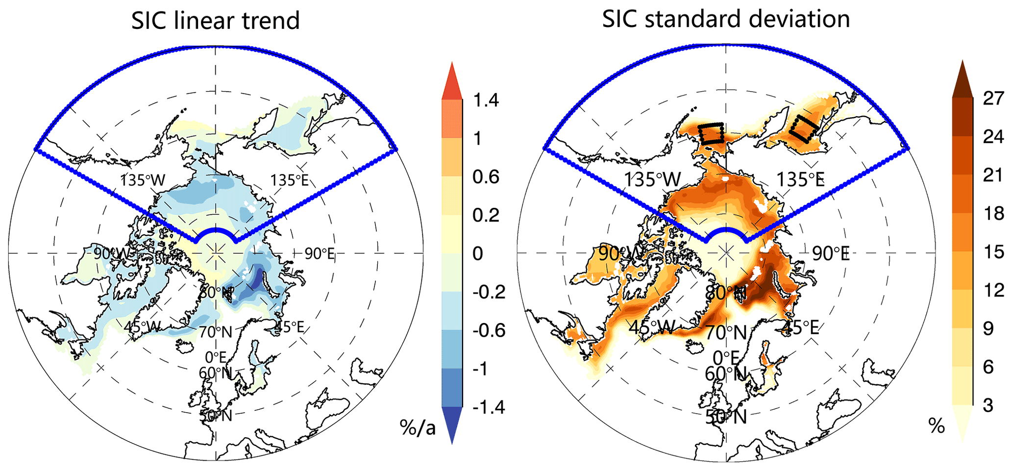
Figure 1 Arctic SIC trends (left) and standard deviation (right) computed using SIC anomalies over all 12 months of the period 1979–2020. The Pacific-Arctic model domain is enclosed by blue lines, which covers 40–84^∘ N and 120–240^∘ E. Two focused areas marked in black boxes in the Bering Sea (58–62^∘ N and 182–192^∘ E) and the Sea of Okhotsk (52–56^∘ N and 144–152^∘ E) have large standard deviations and are selected to evaluate the ACC skill improvement in the regional model compared with the pan-Arctic Markov model developed by Yuan et al. (2016).

3 Model construction and assessments

3.1 EOF analysis of Pacific SIC

Before constructing the model, we first examine whether the EOF analysis can isolate the regional and seasonal SIC variability in the Pacific-Arctic sector. Figure 2 shows the eigenvectors of the three leading EOF modes of SIC. The first mode of SIC variability, accounting for 23 % of the total variance, mainly shows a positive pattern within the Arctic Basin from 1979 to 2002 and a negative pattern after 2003, with a record low in 2007 and 2012, representing the decreasing trend in summer and early fall SIC. The declining trend is heavily loaded inside the Arctic Basin from the East Siberian Sea to the Beaufort Sea. The second SIC mode (9 % of total variance) primarily captures out-of-phase SIC anomalies in the Bering Sea and the Sea of Okhotsk and is associated with the Aleutian–Icelandic low seesaw, representing SIC variability in cold seasons (Frankignoul et al., 2014). This pattern suggests consistently positive SIC anomalies in the Bering Sea and negative anomalies in the Sea of Okhotsk after 2004. The SIC variability in the central sector (approximately 60–70^∘ N) stands out in the third EOF mode (7 % of the total variance), which is a commonly observed feature in the region during spring and autumn. This finding shows that the EOF (MEOF) analysis can well isolate the regional and seasonal SIC variability including the trend in the Pacific-Arctic sector.

We further divided the SIC time series into four seasons and conducted respective EOF analyses. The results show that fewer modes can explain the dominant SIC variance in autumn and summer, benefiting from the large SIC variability and trend (Fig. S1 in the Supplement). For example, the leading 10 modes can explain 70 % of the SIC total variance in autumn and summer, while about 25 modes are needed for explaining the same amount of variance in cold seasons. It turns out that the several leading modes can explain the dominant SIC variability. This is an important premise to reduce the model dimension and, more importantly, to filter out incoherent small-scale features that are likely unpredictable. In addition, it is necessary to build the sea ice prediction model for individual seasons because of the differences in seasonal patterns of variability and the different number of leading modes required to capture predictable variability.

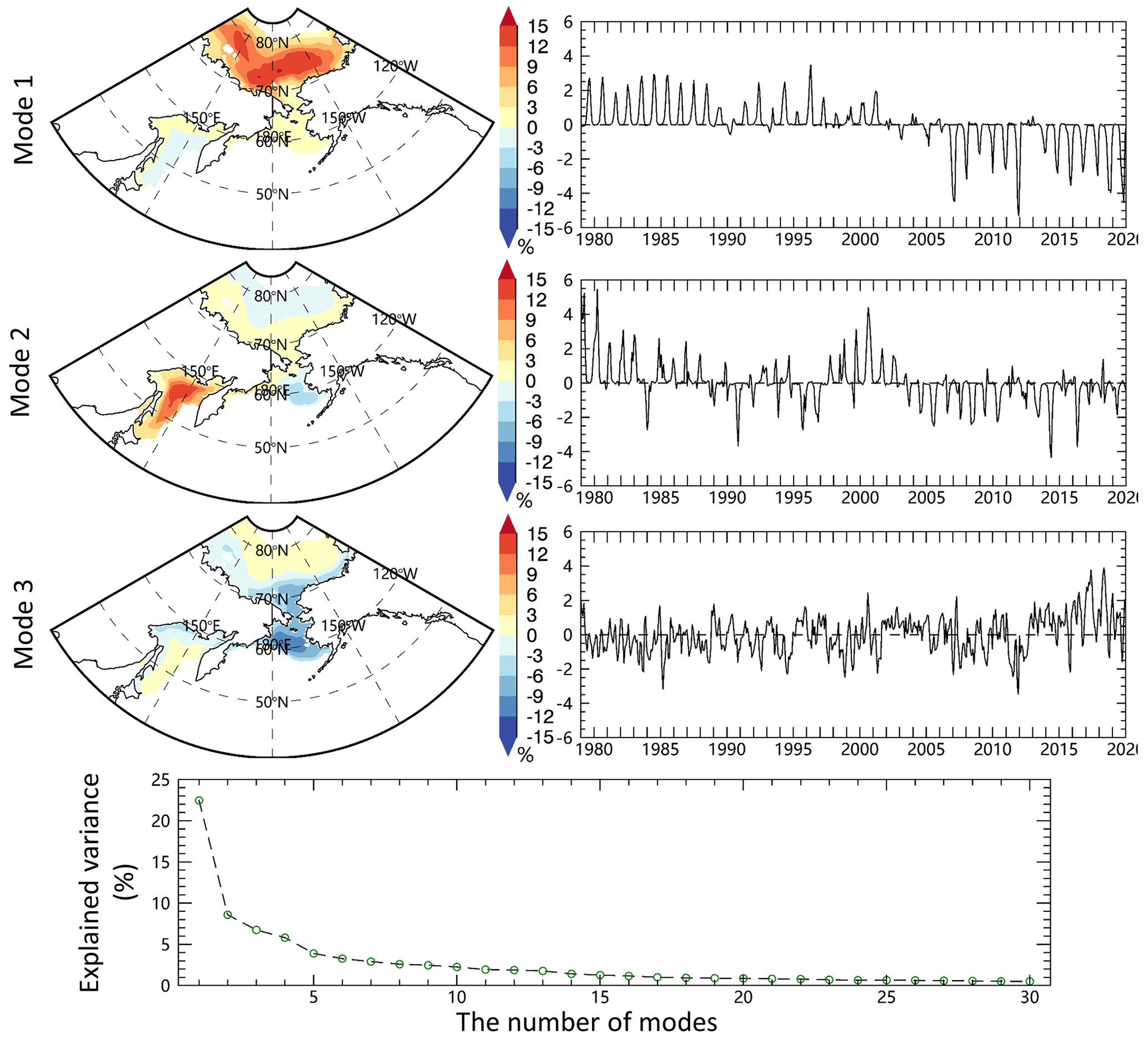
Figure 2 The eigenvectors and PCs of the three leading EOF modes of SIC in the Pacific-Arctic sector for the period 1979–2020. The bottom panel shows the explained variance as a function of the number of leading modes of SIC.

3.2 Construction of an optimal model for each season

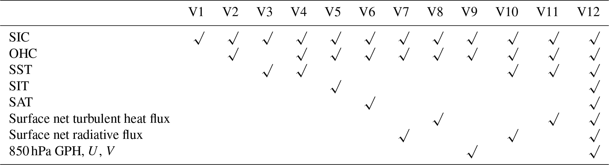
A practical issue in building a Markov model in MEOF spaces is which combination of variables and number of leading modes are to be retained in the model. Using too few modes may miss some predictable signals, and too many may result in overfitting and contaminate the model with incoherent small-scale features. To determine optimal predictor variables and reasonable mode truncations, we calculate the prediction skill from a series of cross-validated model experiments, which used different numbers of modes and different variables. Table 1 shows the detailed variable combinations. Models V2–V4, V6-V8, and V10–V11 are weighted toward thermodynamic processes, whereas V9 and V12 represent integration of thermodynamic and dynamic processes.

Table 1 Variable combinations in cross-validated experiments. V1 represents the no. 1 variable combination. √ represents the variable included in the corresponding combination.

The cross-validation scheme is carried out for the time series to produce predictions at 1- to 12-month leads. The PGS and mean RMSE for each lead time in each season are calculated. To avoid missing predictable signals, we initially retain large amounts of modes (up to 52) in the model and then narrow the range of mode numbers to determine the best model configuration for each season. Figure S2 presents the PGS for each lead time for winter target months. It shows that the model prediction skill in winter steeply decreases after 36 modes in most lead months. Similarly, RMSE increases rapidly after 36 modes (Fig. S3). This indicates that including modes beyond mode 36 in winter, mainly representative of unpredictable small-scale features, leads to the rapid decrease of predictive skill.

To select a model configuration that fits all lead times, we average the 12 panels in Figs. S2 and S3, respectively, and display them in the first column of Fig. S4. Similarly, predictive skills for other seasons are also examined. We further narrow the modes' range to display the predictive skill according to Fig. S4 so that we can determine the optimal model more accurately (Fig. 3). Generally, the model skills are better in summer and autumn than in winter and spring, and more modes are needed in the cold season to capture the predictable signal of SIC, which is likely due to the weaker trends in these months. Models with high correlation also have smaller RMSE but the RMSE differences between models are relatively small.

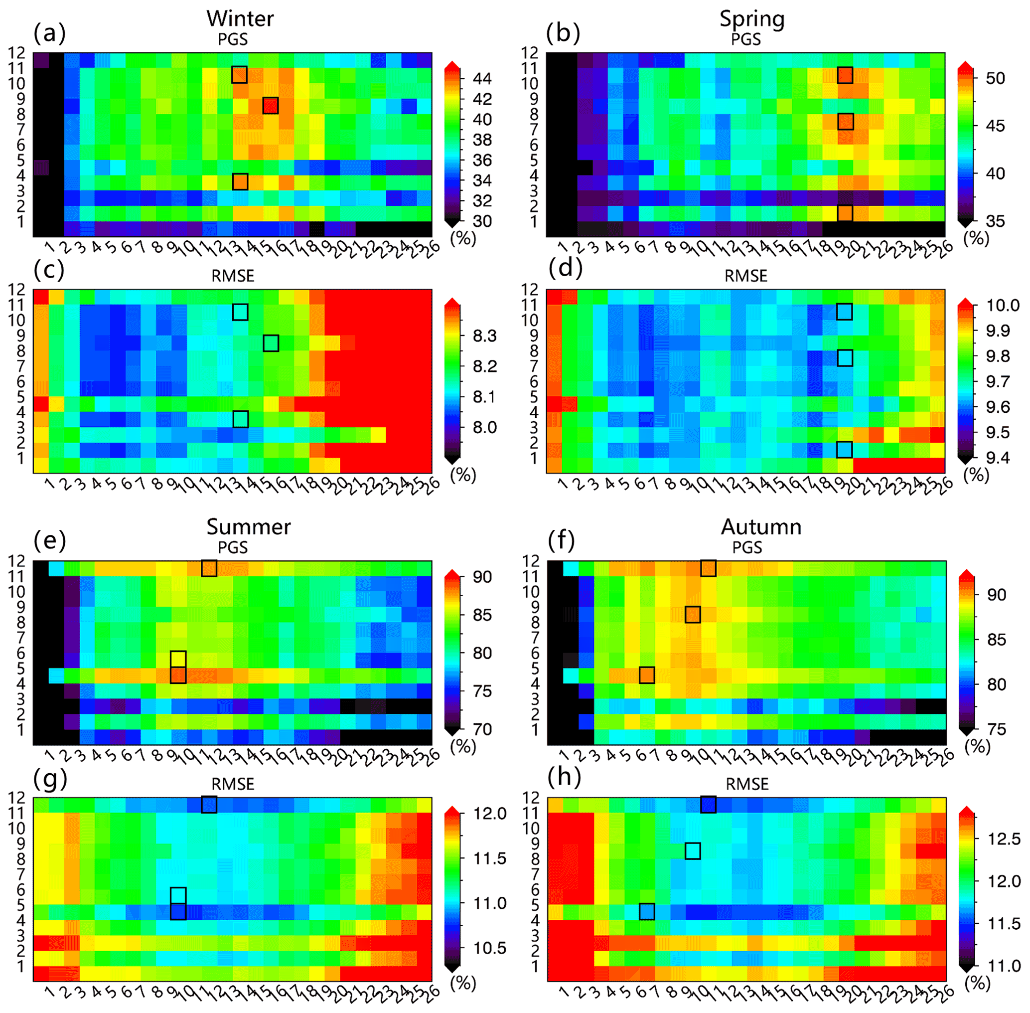
Figure 3 Mean PGS and mean RMSE between the observations and predictions in four seasons. (a) Mean PGS is obtained by averaging all lead months for winter predictions. The x axis represents the number of MEOF modes, and the y axis represents the combination of the variables corresponding to Table 1. Panels (b), (e), and (f) are the same as (a) except for spring, summer, and autumn, respectively. Panels (c), (d), (g), and (h) are the same as (a), (b), (e), and (f) except for RMSE.

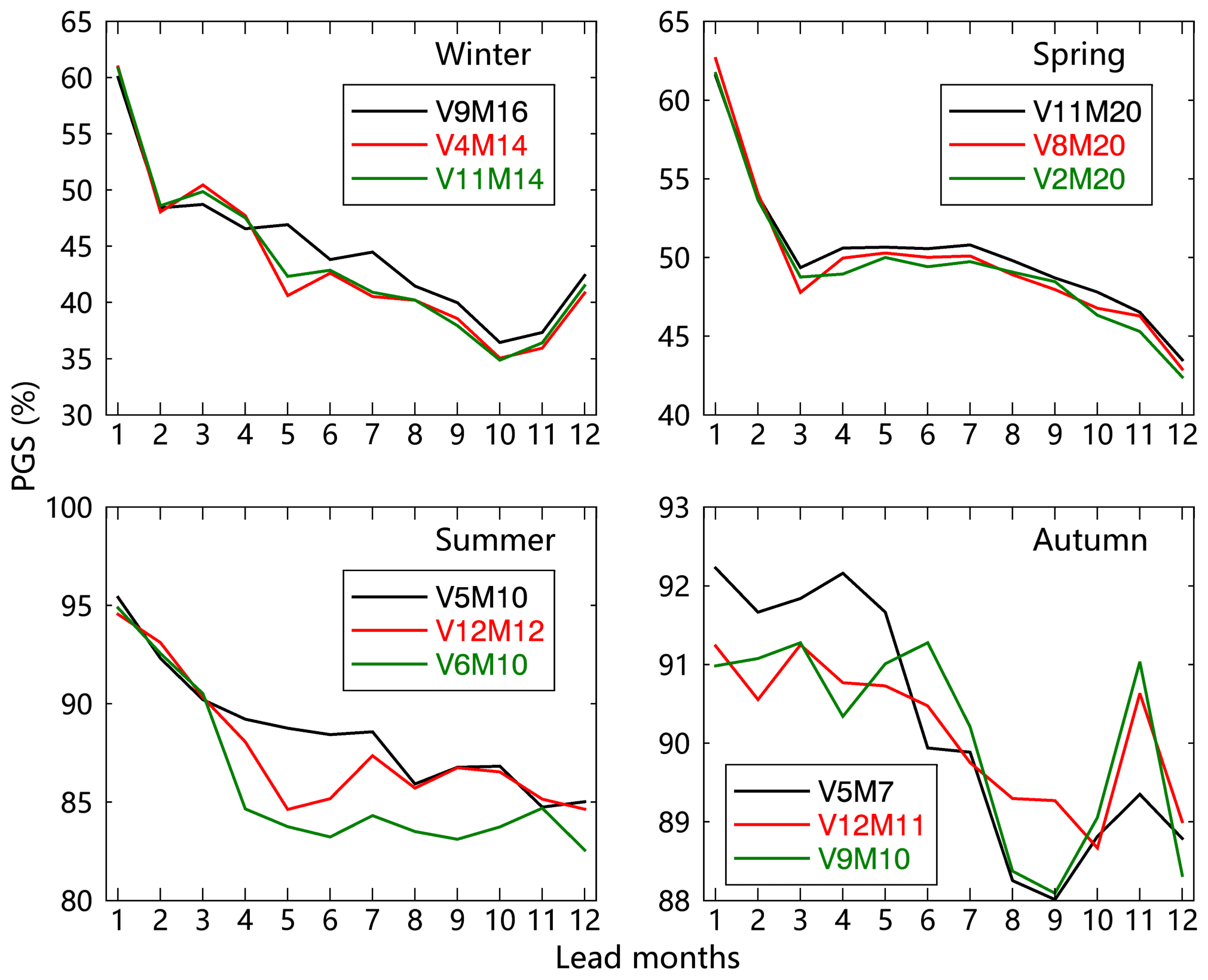
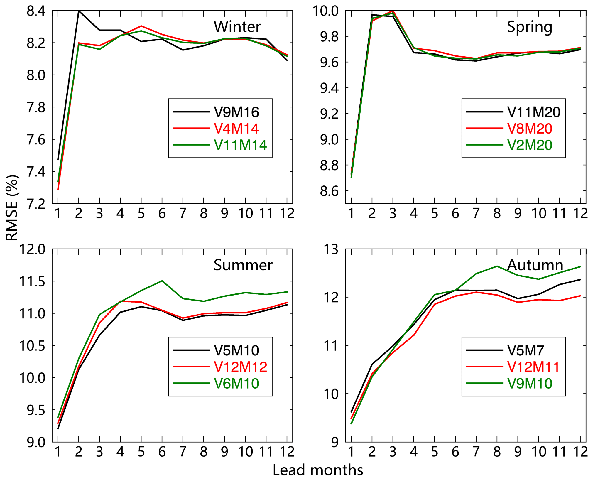
Based on the PGS and RMSE, we primarily chose three superior model configurations marked by black boxes in Fig. 3 for each season, respectively. To determine which model configuration produces the best prediction in each season, we spatially average the SIC prediction skill from these superior models with 1- to 12-month leads (Figs. 4 and 5). Figure 4 shows the cross-validation skill measured by PGS. In general, the predictive skill in the warm season is higher than that in the cold season, although the RMSEs are also relatively large in the warm season (Fig. 5). The model prediction skills based on those superior model configurations have similar variability and magnitude in winter and spring, respectively, while large differences in these occur in the warm season, especially in autumn. It also shows that the model prediction skill steeply decreases at the 2-month lead in winter and at the 2- and 3-month leads in spring.

As a model construction principle, we choose the minimum number of variables and modes to achieve the same level of skill, avoiding possible overfitting. Based on the PGS and RMSE, we chose V9M16 as the best model in winter since it shows the highest PGS. Similarly, we chose V11M20 in spring and V5M10 in summer. In autumn, the model skill from V5 is obviously superior at 1–5 lead months, while V12 dominates prediction skill beyond the 8-month lead. We decided to choose V5M7 because it has a relatively higher mean skill and fewer variables and modes.

The contribution of different variables in ice prediction skill for each season is also assessed. OHC contributes more model prediction skill than SST in all seasons (Fig. 3). The model built on the data matrix of SIC and OHC performs better in winter and spring, which indicates that the OHC provides a considerable source of memory for SIC prediction skill in the cold season and plays a key role in the evolution of sea ice conditions. The results are consistent with many previous studies (Bushuk et al., 2017a; Dai et al., 2020; Guemas et al., 2016b; Lenetsky et al., 2021). 850 hPa GPH and winds can still contribute additional prediction skill in winter since the model with OHC, GPH, and winds slightly outperforms the case without GPH and winds (Fig. 4). 850 hPa GPH and wind not only affect the heat and moisture transported by the atmospheric circulation anomaly but also drive sea ice drift. For example, the dipole structure anomaly of the Arctic atmospheric circulation shows strong meridionality and plays a profound role in sea ice export/import, and heat and moisture transport through the Pacific-Arctic sector (Wu et al., 2006).

Similarly, SST and turbulent heat flux also contribute additional skill in spring although the contribution is minor (Figs. 3 and 4). It is worth mentioning that the variable such as SST with minor additional contributions to the model does not mean that it is a minor contributor since the contributions from different variables to prediction skill partially overlap. In addition, adding SIT to the model has a substantial contribution to the prediction skill in the warm season, indicating that sea ice thickness is a key source of sea ice predictability within the Arctic Basin in the warm season, especially in summer, which is consistent with previous studies (Blanchard-Wrigglesworth et al., 2011; Blockley and Peterson, 2018; Day et al., 2014a; Morioka et al., 2021; Tian et al., 2021; Yuan et al., 2016). However, SIT has a negative contribution to the prediction skill in the cold season (Fig. 3). The contributions of SIT to the prediction skill in autumn are very sensitive to the number of lead months in that the skill steeply decreases beyond a 5-month lead (Fig. 4). In other words, the model did not perform well in autumn prediction initialized in winter and spring. In addition, the surface net radiative flux also contributes to the model skill in the cold season (Fig. 3). Early studies suggested that the surface longwave radiation plays an indispensable role in the polar climate system in the cold season when shortwave radiation is at its annual minimum (Huang et al., 2015; Kapsch et al., 2013; Lee et al., 2017; Liu and Key, 2014; Luo et al., 2017; Y. Wang et al., 2019).

Figure 4 PGS for the preliminary selection of superior models in each season.

Figure 5 Same as Fig. 4 but for RMSE.

3.3 Assessment of model skill

To test the forecast skill of the model, the SIC predictions were evaluated at each grid cell and for all seasons using the ACC and RMSE between predicted and observed anomalies, and the skill is presented at 3, 6, 9, and 12 lead months. In winter (DJF), high forecast skill is concentrated in the Arctic marginal seas and peripheral seas: the southern Chukchi Sea and Sea of Okhotsk (Fig. 6). The skill is slightly lower at a 12-month lead in the Sea of Okhotsk and a 9-month lead in the southern Chukchi Sea. Overall, the winter skill is roughly 0.4 in the Sea of Okhotsk and 0.5 in the southern Chukchi Sea at leads of up to 12 months. The spring (MAM) prediction skill shows a similar pattern to that in winter but with a 0.1 increase in the ACC skill. The southern Chukchi Sea and Bering Strait have higher skills than the Bering Sea. For summer (JJA) predictions, the prediction skill is concentrated in the Arctic basin since sea ice totally melts in the Arctic peripheral seas. The 3-month lead prediction has the highest skill (> 0.6) in most of the Arctic basin, while the lowest prediction skill (< 0.5) is found at a 12-month lead. The autumn (SON) prediction skill shows a similar pattern to the summer skill but with higher correlations. In general, the model has higher prediction skills for warm seasons, especially for autumn, than that for cold seasons, while the lowest skill is in winter.

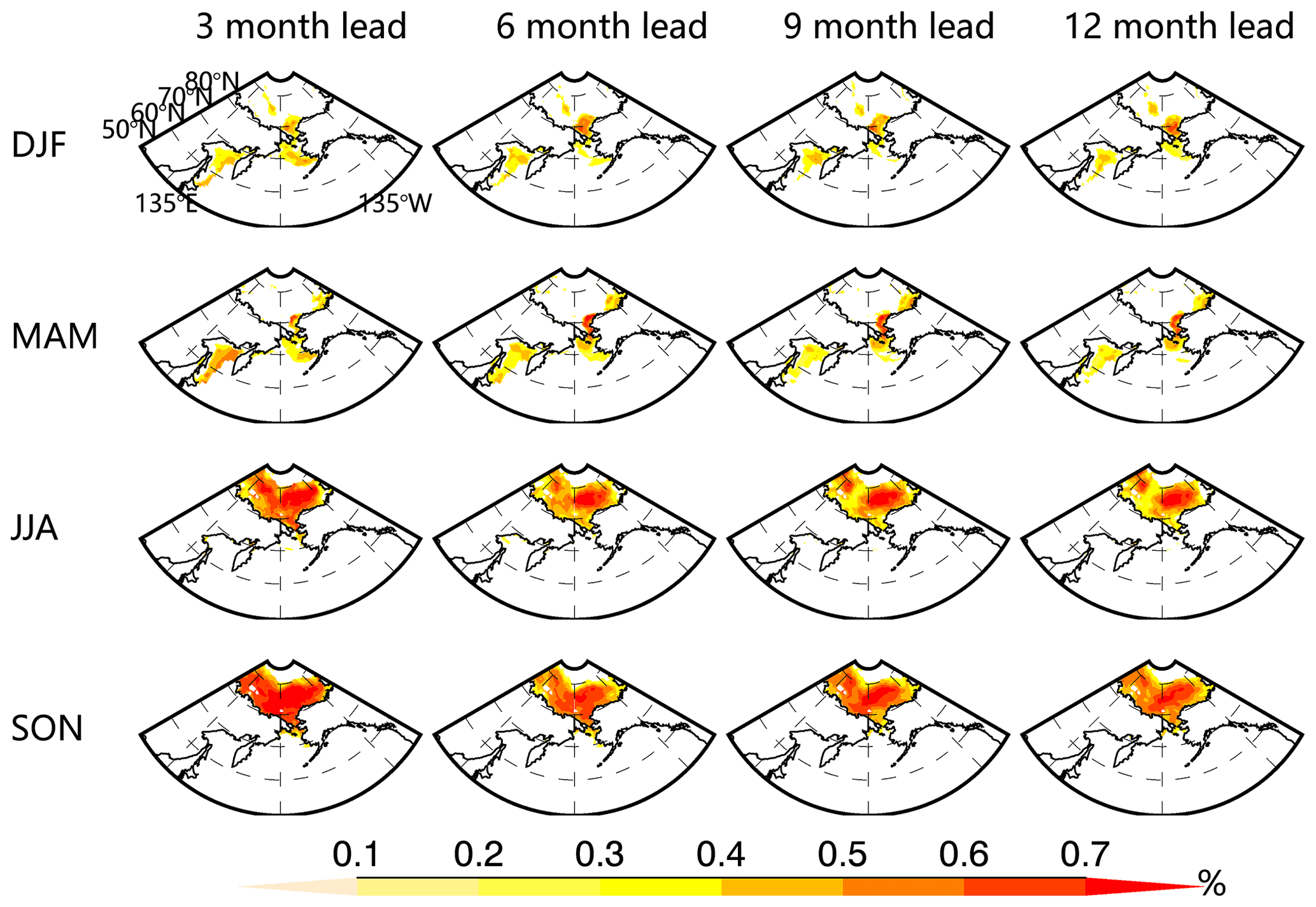
Figure 6 Cross-validated model skills measured by ACC between SIC predictions and observation anomalies as a function of seasons and lead months. Only the correlations that are significantly above the 95 % confidence level based on Student's t test are included in the panels.

RMSEs are consistent with correlations: high correlations correspond to low RMSEs, and vice versa, although minor inconsistencies occur in some seasons and regions (Fig. 7). The RMSE is large around the Arctic basin for the warm season and in the peripheral sea for the cold season where SIC has large variability. In the cold season, the RMSE is larger in the Bering Sea than that in the Sea of Okhotsk. The magnitudes of RMSE remain at roughly the same level from 3- to 12-month leads in most locations for all seasons. The marginal seas have larger RMSEs than the central Arctic basin in both summer and autumn, while the error magnitudes in autumn are slightly larger than those in summer but smaller than the SIC standard deviation across the Pacific sector (Fig. 1).

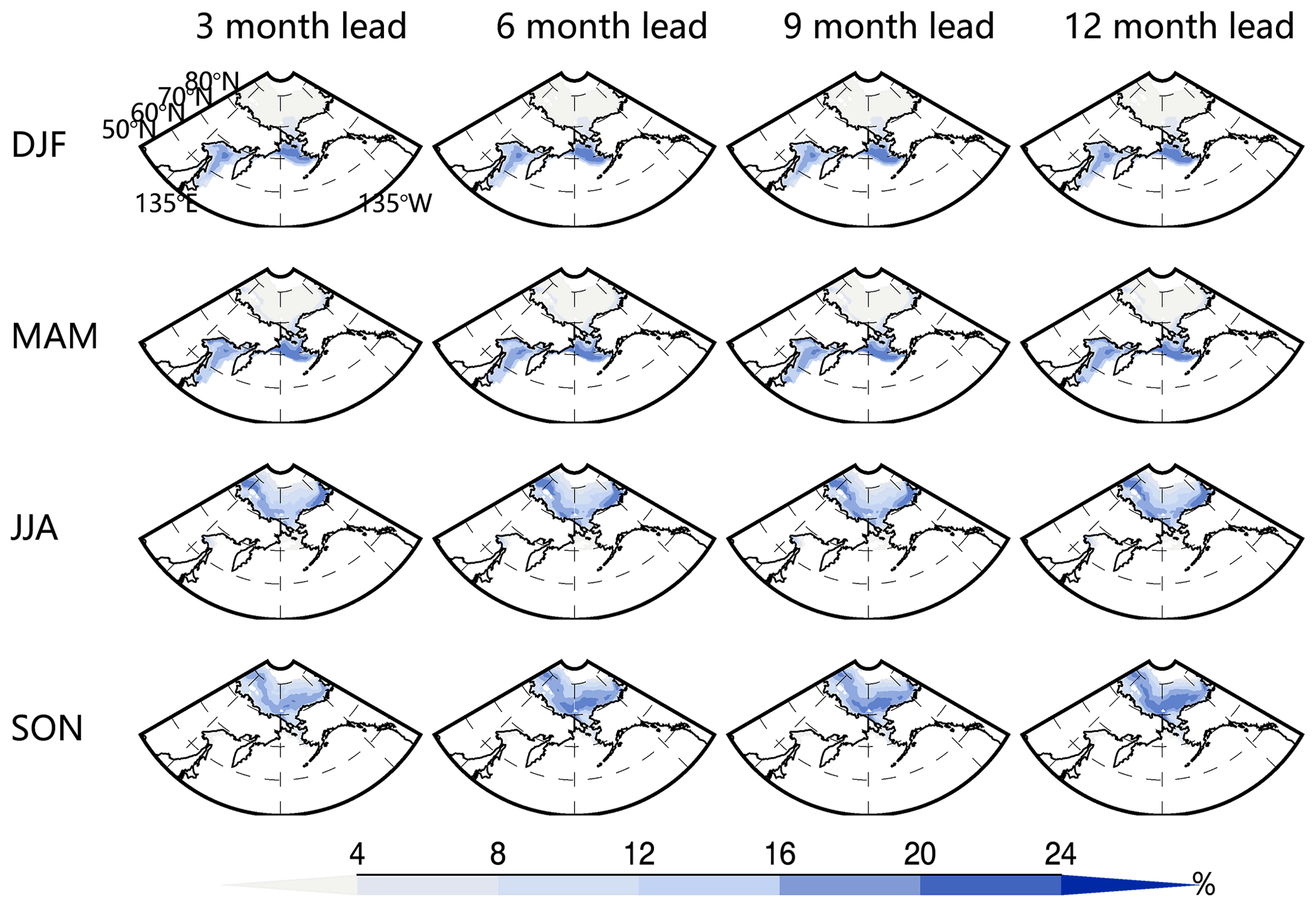
Figure 7 Same as Fig. 6 except for RMSEs. The color bar is in a unit of percentage.

Also, the model performance is further evaluated against anomaly persistence and climatology. Averaged over the grid points in the model domain and over all seasons for the period of 1980–2020, the regional Markov model's mean correlation is manifestly higher, and the mean RMSE of the regional Markov model is much lower than the climatology and anomaly persistence for all the lead months, especially from 2- to 10-month leads (Fig. 8). In addition, RMSE is not sensitive to the lead months, showing the superiority of the regional model. These results suggest that the regional Markov model can capture significantly more predictability beyond SIC anomaly persistence.

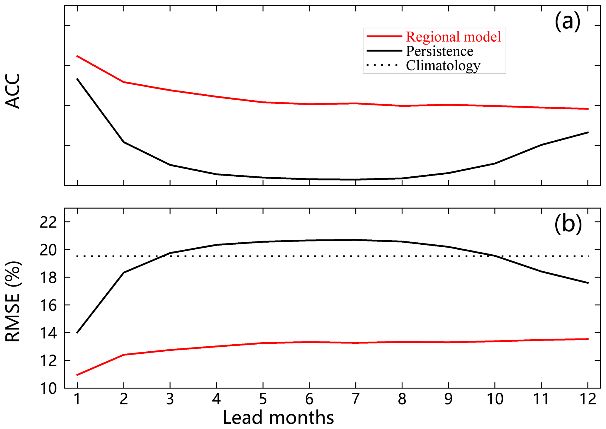
Figure 8 The prediction skill of the regional Markov model compared against that of anomaly persistence and climatology averaged over the model domain as a function of the number of months of lead time.

To assess the regional model skill improvements from the pan-Arctic model presented by Yuan et al. (2016), we calculated the ACC as a function of lead months (Fig. 9). Note that the ACC is calculated only in typical regions with large standard deviations marked in Fig. 1. The regional model evidently enhances the ACC skill from the pan-Arctic model for the 4- to 12-month lead predictions in the Bering Sea and the 1- to 7-month lead predictions in the Sea of Okhotsk. The mean ACC is also increased by 32 % in the Bering Sea and by 18 % in the Sea of Okhotsk. The prediction skill of the regional Markov model within the Arctic basin also remains at the same high level as that of the pan-Arctic model (not shown), so significant skill improvements occur in the peripheral sea of the Pacific sector.

Figure 9 Cross-validated model skills of the regional Markov model vs. the pan-Arctic Markov model. (a) The skills are measured by the ACC between predictions and observations with trends from 1980 to 2020 as a function of lead months in the Bering Sea. Panel (b) is the same as (a) except for the Sea of Okhotsk. The red numbers in the bottom left of each panel represent the mean regional model skill improvements from the pan-Arctic model.

4 Discussion

4.1 Contribution of linear trends to SIE prediction skill

Sigmond et al. (2013) show that the linear trend in Arctic SIE dramatically contributes to its forecast skill to CanSIPS. Lindsay et al. (2008) show that their dynamic model prediction skill is much lower when the trend is not included. They suggested that the trend accounts for 76 % of the variance of the pan-Arctic ice extent in September. The trend also contributes to the pan-Arctic prediction in the linear Markov model (Yuan et al., 2016). In the Arctic, SIE has declined at −0.35 million square kilometers per decade during 1979–2020, which is significant at the 95 % confidence level. The large SIC trend is mainly in the Barents Sea and the Kara Sea, followed by the Chukchi Sea, while the mean SIC trend in the Bering Sea and the Sea of Okhotsk is relatively weak (Fig. 1). To evaluate the contribution of long-term trends to the regional Markov model skill, we conducted post-prediction analysis on the linear trends' contribution to the predictions skill of SIE in the Pacific-Arctic sector. We examine the time series of SIE in all calendar and lead months calculated by summing the Pacific-Arctic areas that have at least 15 % SIC from observations and predictions. Monthly trends were removed from the predictions and observations, respectively. Then, the model skill is compared between the original SIE predictions and detrended SIE predictions.

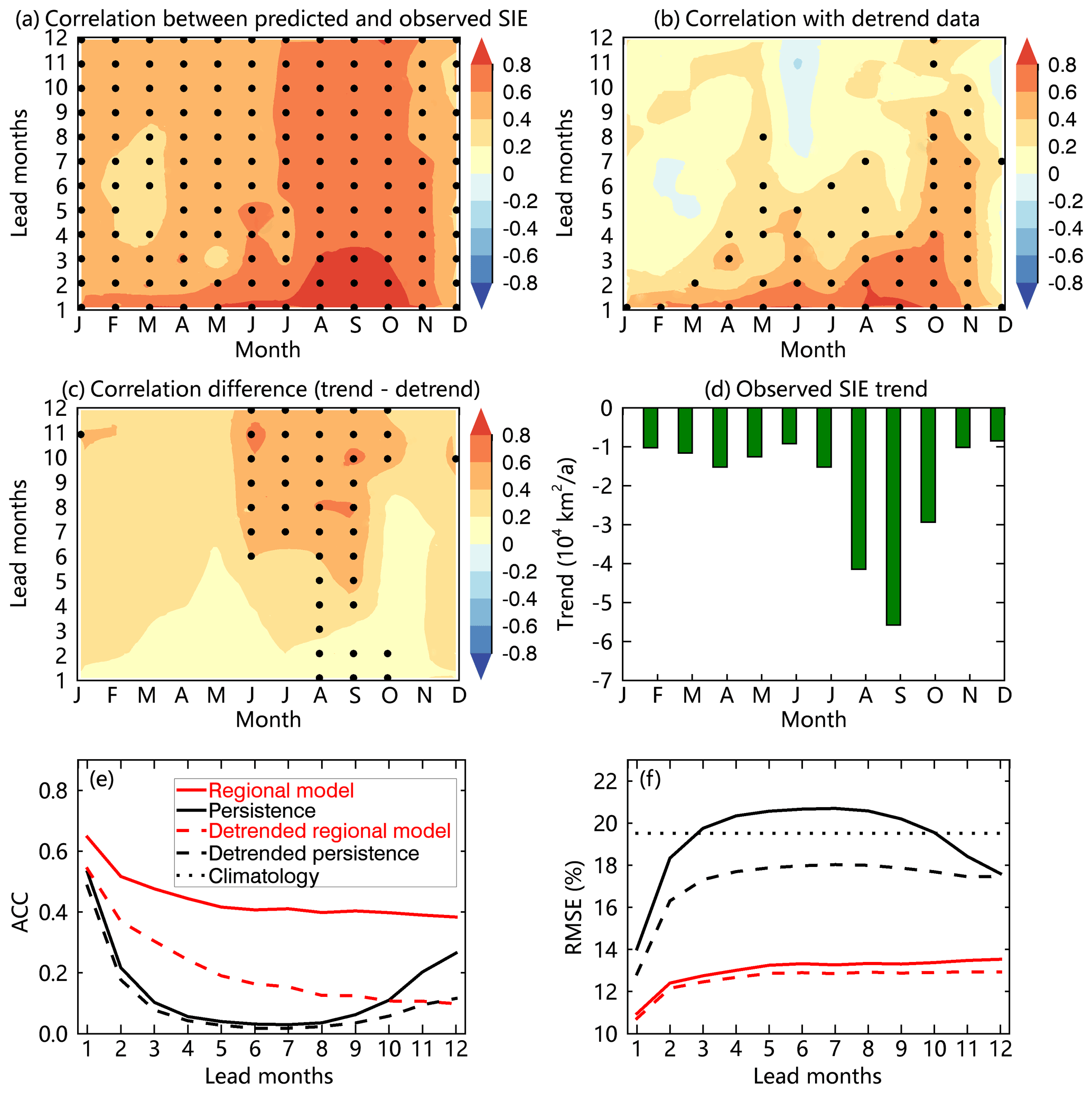
Figure 10 (a) The SIE forecast skill of the regional Markov model as a function of the calendar month and lead months. (b) The SIE forecast skill when monthly trends are removed from the predictions and observations, respectively. The black dots in (a) and (b) represent the correlations that are significantly above the 95 % confidence level. (c) Difference between (a) and (b). The black dots in (c) indicate that the correlation differences are significant above the 95 % confidence level. (d) Observed trends in SIE as a function of the calendar month. All monthly SIE trends are significantly above the 95 % confidence level. (e, f) The prediction skill of the regional Markov model compared against that of anomaly persistence and climatology averaged over the model domain as a function of the number of months of lead time.

The model is skillful in predicting SIE from January to November at a 1-month lead (Fig. 10a). The skill is particularly high for summer and autumn predictions, where ACC is higher than 0.6 from July through November even at a 12-month lead. The model skill is relatively low in May, especially at 4–8 lead months. This pattern is consistent with the seasonal variation of the model skill for SIC prediction presented in Fig. 6. After monthly trends are removed from predictions and observations, respectively, the model skill is significantly reduced for all seasons, especially for the warm season at 6–12 lead months (Fig. 10b, c). This is consistent with the seasonality of the observed trend (Fig. 10d), which also peaks in late summer and early fall.

Averaging the differences in Fig. 10c over all lead times and predicted months, the trend removal results in a mean reduction of 0.31 from the SIE forecast skill and a 53 % reduction of the mean ACC. However, the model retains high prediction skill (0.61) from January to November at 1–2 lead months, representing a 19 % reduction by the trend removal (Fig. 10b), which shows the model's capability of capturing sea ice internal variability. In addition, the trend is relatively large in the Chukchi Sea and weak outside of the Arctic Ocean. The model only reduces 13 % of the mean ACC from January to November at 1–2 lead months after the trend removal for the area outside of the Arctic Ocean. Although linear trends contribute significantly to the model skill, the regional Markov model's mean correlation is manifestly higher, and the mean RMSE of the regional Markov model is much lower than the climatology and anomaly persistence for all the lead months when the sea ice trend is removed (Fig. 10e, f).

4.2 Comparison with the GFDL model

Yuan et al. (2016) showed that the pan-Arctic Markov model consistently outperforms the NOAA/NCEP Climate Forecast System (CFSv2) and CanSIPS for sea ice seasonal predictions. Here the regional Markov model is compared with the Geophysical Fluid Dynamics Laboratory Forecast-oriented Low Ocean Resolution (GFDL-FLOR) seasonal prediction system (Bushuk et al., 2017a) in detrended SIE forecasts. The hindcast model skills measured by the ACC for detrended SIE are high from both the regional Markov model and GFDL model from January to June at 1- to 3-month leads in the Pacific sector (Fig. 11). The regional Markov model skill is statistically significant at lead times ranging from 1 to 6 months for the target months of January–June in both the Bering Sea and the Sea of Okhotsk. Below we highlight some key differences between these two models in the Bering Sea and the Sea of Okhotsk.

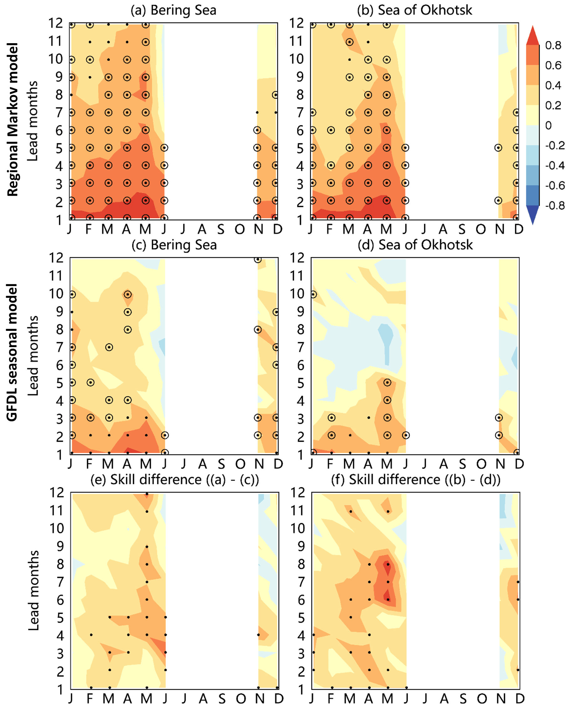
Figure 11 (a, b) Hindcast model skill (ACC) for detrended regional SIE forecasts from 1982 to 2020 for the regional Markov model. (c, d) Same as (a, b) except for the GFDL seasonal prediction system. Panels (e, f) show the skill difference between these two models. The black dots in (a)–(d) represent ACCs that are significantly above the 95 % confidence level, and the circles in (a)–(d) indicate months in which the model's skill exceeds that of a persistence forecast. The black dots in (e)–(f) represent ACC differences that are significant above the 95 % confidence level.

Notably, the skill from the regional Markov model is higher than that from the GFDL seasonal prediction system from February to June at 3- to 6-month leads in the Bering Sea and from December to June at 1- to 8-month leads in the Sea of Okhotsk. In other words, the regional Markov model performs better in spring prediction using winter observations for the Bering Sea and autumn observations for the Sea of Okhotsk. Nevertheless, the regional Markov model slightly underperforms the GFDL seasonal prediction system in predictions from November to December using the previous winter and spring observations for the Bering Sea and using the previous winter observations for the Sea of Okhotsk. Overall, the regional Markov model delivers skillful SIE predictions in seasonal ice zones of the Pacific sector up to 7-month lead times, an improvement from the 3-month leads displayed in the GFDL seasonal prediction system.

4.3 Sensitivity of model domain in the prediction skill

We conducted a sensitivity analysis of the model domain in the prediction skill in the Bering Sea and the Sea of Okhotsk with the same model configuration and different sizes of the model domain. The model domain is defined by 90 to 270, 120 to 240, and 135 to 225^∘ E, respectively. The results show that the prediction skill patterns based on three model domains show high similarity in the Bering Sea and the skill based on the model domain (120 to 240^∘ E) is highest at all month leads. The prediction skill in the Sea of Okhotsk based on the model domain (135 to 225^∘ E) is highlighted at 5- to 8-month leads, but is poor at 11- to 12-month leads. Although the models with different sizes of model domain have different prediction skills in the Bering Sea and the Sea of Okhotsk, the differences are not significant because all those model domains contain highly similar signals of climate variability. Therefore, the regional model is not highly sensitive to the size of the model domain within the Pacific-Arctic sector.

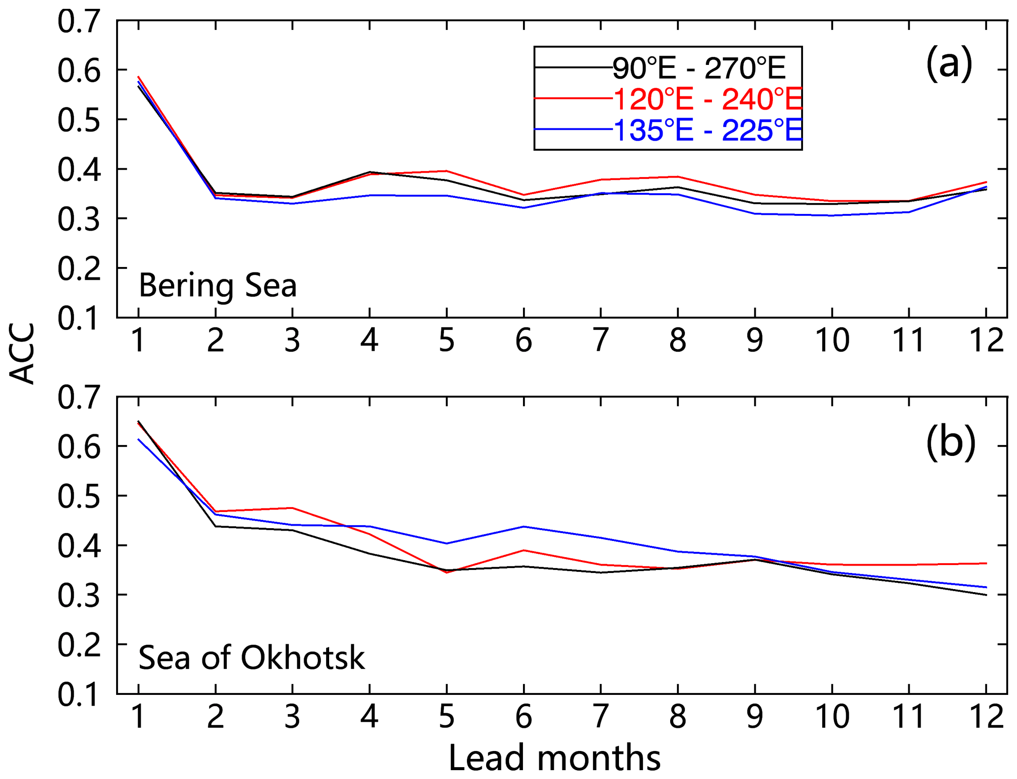
Figure 12 Cross-validated model skills of the regional Markov model with the same model configuration and different sizes of the model domain. (a) The skills are measured by the ACC between predictions and observations with trends from 1980 to 2020 as a function of lead months in the Bering Sea. Panel (b) is the same as (a) except for the Sea of Okhotsk. The model is configured by V9M16 in winter, V11M20 in spring, V5M10 in summer, and V5M7 in autumn. The ACC values are averaged over the area marked in the black box in Fig. 1.

5 Conclusions

Here, we developed a regional Markov model to predict SIC in the Pacific-Arctic sector at the seasonal timescale. The model was constructed in the MEOF space so that it can capture the covariability of the North Pacific climate system defined by nine variables (SIC, OHC, SIT, SST, SAT, surface net radiative flux, surface net turbulent heat flux, and GPH and winds at 850 hPa). Based on cross-validation experiments, we selected model variables and mode truncations that provided the best results in each season. These model configurations were V9M16 for winter, V11M20 for spring, V5M10 for summer, and V5M7 for autumn.

The SIC prediction skill was evaluated at each grid cell and for all seasons using ACC. The regional Markov model's skill is superior to the skill derived from anomaly persistence, revealing the model's ability to capture more predictable SIC internal variability than anomaly persistence. The winter skill is about 0.4 in the Sea of Okhotsk and 0.5 in the northern Bering Sea at leads of up to 12 months. The spring prediction shows a similar pattern but with a 0.1 increase in the ACC skill. The model skill in summer and autumn is more than 0.6 within the Arctic basin. Compared with the pan-Arctic seasonal prediction model, the regional Markov model distinctly improves the SIC prediction skill in the peripheral seas of the Pacific-Arctic sector. The regional model significantly enhances the correlation skill from the pan-Arctic model for 4- to 12-month lead predictions in the Bering Sea and 1- to 7-month lead predictions in the Sea of Okhotsk. The improvement is a 32 % ACC increase in the Bering Sea and 18 % in the Sea of Okhotsk. In addition, similar to the pan-Arctic Markov model, the regional model is not sensitive to the number of MEOF modes retained, which indicates that the performance of this Markov model is robust.

The model retains prediction skill whether the sea ice trend is removed or not. However, the detrended skill is notably lower, consistent with earlier sea ice prediction studies. When sea ice time series includes the trend, the model can skillfully predict SIE from January to November. The skill is particularly high for the predictions of summer and autumn sea ice at longer lead times, especially in July to November when the skill is > 0.6 even at a 12-month lead. Conversely, in May, the model skill is relatively low, especially at 4–8 lead months. Trend removal from predictions and observations results in a 53 % reduction of the mean ACC for the entire Pacific-Arctic sector. However, the model only reduces 13 % of the mean ACC from January to November at 1–2 lead months after the trend removal in the Bering Sea and the Sea of Okhotsk. This detrended analysis shows the model's capability of capturing sea ice internal variability beyond linear trends. Furthermore, the regional Markov model improves the detrended SIE prediction skill in the Pacific-Arctic sector to 7-month lead times from the 3-month lead skill displayed in the GFDL-FLOR seasonal prediction system.

The following reasons contribute to the improvements. First, the dominant climate variability in the northern middle-to-high latitudes mostly occurs in the Atlantic sector of the Arctic and Subarctic, which dictates the leading MEOF mode in the pan-Arctic model. The unique characteristics of the coupled atmosphere–ocean–sea ice relationships in the Pacific sector may not be included in the leading MEOF decompositions of the pan-Arctic climate system and thus are not correctly represented in the model. The regional model focuses on the Pacific-Arctic coupled atmosphere–ocean–sea ice system and captures the dominant regional climate variability. Second, the Pacific sector of the Arctic needs a different set of variables to maximize the model's predictability. We added OHC and SIT in the regional model, which provides a crucial source of predictability in winter and summer months, respectively. We also include 850 hPa GPH and winds to represent dynamic atmospheric processes in winter and include turbulent heat flux to improve the model skill in spring. Finally, we constructed a superior model for each season, isolating the seasonally dominant processes separately.

It was also found that more modes were needed in the cold season to capture the predictable signal of SIC. This suggests that sea ice in cold seasons has more variability patterns compared with that in warm seasons, which may bring more errors in prediction. SIC trends are strongest in the warm season months, which may contribute to the smaller number of modes required. In addition to the climate system in the Arctic Basin, the coupled atmosphere–ocean–sea ice variability in the North Pacific plays a more important role in the cold season and needs more modes to capture the covariability signals.