the Creative Commons Attribution 4.0 License.
the Creative Commons Attribution 4.0 License.
 | 15 Mar 2022
Evaluation of Northern Hemisphere snow water equivalent in CMIP6 models during 1982–2014
Petri Räisänen
Kari Luojus
Anna Luomaranta
Aku Riihelä
Seasonal snow cover of the Northern Hemisphere (NH) is a major factor in the global climate system, which makes snow cover an important variable in climate models. Previously, substantial uncertainties have been reported in NH snow water equivalent (SWE) estimates. A recent bias-correction method significantly reduces the uncertainty of NH SWE estimation, which enables a more reliable analysis of the climate models' ability to describe the snow cover. We have intercompared NH SWE estimates between CMIP6 (Coupled Model Intercomparison Project Phase 6) models and observation-based SWE reference data north of 40∘ N for the period 1982–2014 and analyzed with a regression approach whether model biases in temperature (T) and precipitation (P) could explain the model biases in SWE. We analyzed separately SWE in winter and SWE change rate in spring. For SWE reference data, we used bias-corrected SnowCCI data for non-mountainous regions and the mean of Brown, MERRA-2 and Crocus v7 data for the mountainous regions. The SnowCCI SWE data are based on satellite passive microwave radiometer data and in situ snow depth data. The analysis shows that CMIP6 models tend to overestimate SWE; however, large variability exists between models. In winter, P is the dominant factor causing SWE discrepancies especially in the northern and coastal regions. T contributes to SWE biases mainly in regions, where T is close to 0∘ C in winter. In spring, the importance of T in explaining the snowmelt rate discrepancies increases. This is to be expected, because the increase in T is the main factor that causes snow to melt as spring progresses. Furthermore, it is obvious from the results that biases in T or P cannot explain all model biases either in SWE in winter or in the snowmelt rate in spring. Other factors, such as deficiencies in model parameterizations and possibly biases in the observational datasets, also contribute to SWE discrepancies. In particular, linear regression suggests that when the biases in T and P are eliminated, the models generally overestimate the snowmelt rate in spring.
- Article
(19649 KB) - Full-text XML
-
Supplement
(23598 KB) - BibTeX
- EndNote


Seasonal snow cover of the Northern Hemisphere (NH) is an important factor of the global climate system. The seasonal snow cover greatly influences surface albedo and, thus, the Earth's energy balance (Callaghan et al., 2011; Flanner et al., 2011; Qu and Hall, 2005; Trenberth and Fasullo, 2009). This makes snow cover an important variable in climate models (Derksen and Brown, 2012; Loth et al., 1993). Additionally, snow cover significantly affects the hydrological cycle at high latitudes and in mountainous regions (Barnett et al., 2005; Bormann et al., 2018; Callaghan et al., 2011; Douville et al., 2002). In winter, snow cover stores large amounts of fresh water, which limits water availability. In spring and summer, warming temperatures melt the snowpack, releasing water as runoff. In some areas, snow is the largest freshwater storage, and about one-sixth of the world's population is dependent on meltwater from snow (Barnett et al., 2005; Hall et al., 2008).
Melting snow is also a major source for hydropower (Callaghan et al., 2011; Magnusson et al., 2020). Due to the global warming, the melting season begins earlier, with the timing of streamflow peaks also becoming earlier (Kundzewicz et al., 2008). In addition, changes in snow cover affect the intensity of spring streamflow, as an increasing proportion of winter precipitation is rain instead of snow (Callaghan et al., 2011; Cohen et al., 2015; Dong et al., 2020; Kundzewicz et al., 2008). Thus, changes in snow cover affecting the hydrological cycle can cause regional water shortages and affect hydropower production.
SWE (snow water equivalent) is the amount of water contained in the snowpack (in units of kg m−2) or, equivalently, the height of the water layer (in units of mm) that would result from melting the whole snowpack instantaneously (Fierz et al., 2009). Recent studies show negative trends in global SWE (Bormann et al., 2018; Derksen and Brown, 2012; Essery et al., 2020; Hernández-Henríquez et al., 2015; Mortimer et al., 2020; Mudryk et al., 2017), but significant spatial variability exists: North America shows clear negative trends in observed SWE, while negative trends are less pronounced in Eurasia (Kunkel et al., 2016; Pulliainen et al., 2020). At mid-latitudes, SWE is more sensitive to warming than at high latitudes (Brown and Mote, 2009). Although the overall SWE trends are negative, there are also regions where SWE is observed and projected to increase: SWE will most likely increase in northern Siberia and northern Canada, which largely results from the increased atmospheric moisture holding capacity (Brown and Mote, 2009; Park et al., 2012; Räisänen, 2008). Trends in snow cover also vary seasonally: the seasonal snow in spring is especially sensitive to warming due to the strong surface albedo feedback, and the observed snow cover trends in spring are clearly negative in both Eurasia and North America (Derksen and Brown, 2012; Essery et al., 2020; Hernández-Henríquez et al., 2015). In winter, the observed trends are less pronounced: early winter from October to December shows even slightly positive trends in both Eurasia and North America, while in January and February, there are no significant trends (Hernández-Henríquez et al., 2015).
Observing SWE at continental scale is only possible from satellites, but also model and reanalysis products provide gridded SWE estimates which have been widely used in hydrological and climate research (e.g., Huning and AghaKouchak, 2020; Mortimer et al., 2020; Mudryk et al., 2020). Previously, substantial uncertainties have been reported in the NH SWE estimates (Bormann et al., 2018; Mudryk et al., 2015). However, our knowledge of the NH SWE has recently improved considerably with new bias corrections which reduce the uncertainty of the SWE estimate integrated over NH from 33 % to 7.4 % (Pulliainen et al., 2020). The bias-correction method, for example, considerably improves SWE estimates in the moderate and deep SWE range (Pulliainen et al., 2020), which has previously caused underestimation in SWE estimates (Cho et al., 2020). However, limitations still exist: the bias-correction method cannot be applied in mountainous regions due to the lack of snow course measurements and the large SWE variability in complex terrain (Pulliainen et al., 2020). Even though the area of mountainous regions is limited, these regions store a considerable portion of seasonal snow (Kim et al., 2021). For observation-based datasets, the bias-correction method mostly increases SWE, and it is therefore likely that without bias-correction or alternative approaches where estimates are corrected using in situ data, SWE in mountainous areas is underestimated (Pulliainen et al., 2020; Wrzesien et al., 2018).
Previous studies have shown that climate models have had difficulties in correctly reproducing the seasonal snow and its recent trends (Brutel-Vuilmet et al., 2013; Derksen and Brown, 2012; Henderson et al., 2018; Santolaria-Otín and Zolina, 2020; Thackeray et al., 2016). However, there are clear improvements from CMIP5 to CMIP6. The snow cover extent is better described in CMIP6 than in CMIP5 models (Mudryk et al., 2020; Zhu et al., 2021). The snow cover fraction is underestimated in both CMIP5 and CMIP6 multi-model ensemble means, but the biases are clearly smaller in CMIP6 than in CMIP5 (Zhu et al., 2021). SWE, in turn, is biased high in both CMIP5 and CMIP6, and the peak SWE is also overestimated in almost all models (Mudryk et al., 2020). The model biases also vary seasonally; the snow cover fraction is best described in the period from January to March in CMIP6 models (Zhu et al., 2021), whereas the SWE bias is smallest in autumn and early winter and increases in spring (Mudryk et al., 2020). Both CMIP5 and CMIP6 models are mostly able to reproduce the observed negative trend in snow cover area, but there are uncertainties in the magnitude of the trend (Mudryk et al., 2020; Zhu et al., 2021). The CMIP5 models are able to better capture the trend in snow cover extent than the trend in SWE (Santolaria-Otín and Zolina, 2020).
Due to the reasons described above, it is crucial that seasonal snow is accurately described in climate models to properly predict the state of the cryosphere in future climate. Therefore, it is important to study how the new CMIP6 climate models can describe the seasonal snow, as well as where the uncertainties and discrepancies arise. The current paper focuses on the climatological distribution of SWE in CMIP6 models. To our knowledge, only one previous study has evaluated NH SWE in CMIP6 models: Mudryk et al. (2020) compared SWE estimates between CMIP6 models and several observational datasets. Additionally, they studied the connection between SWE and temperature but did not consider temperature and precipitation together. However, they stated that a coordinated analysis of temperature and precipitation is needed to determine SWE trend drivers. In general, simulated trends of SWE can be considered more reliable if the current climatological distribution of SWE is simulated accurately. Therefore, in the present study, we consider, for the first time, the role of both temperature and precipitation for SWE biases in CMIP6 climate models. Specifically, the main goals of this study are (1) to intercompare the CMIP6 and observation-based SWE estimates and (2) to analyze whether temperature and precipitation biases could explain the SWE biases.
2.1 CMIP6 model data
The data of this study consist of CMIP6 climate model data (Table 1) and observational and reanalysis data (Table 2). For CMIP6, we used monthly mean data from those models for which either historical or esm-hist simulations were available for download in August 2021. The historical and esm-hist simulations extend from 1850 to 2014. In historical simulations, the CO2 concentrations are prescribed, whereas in esm-hist simulations, the models calculate the atmospheric CO2 concentration interactively based on prescribed CO2 fluxes (Eyring et al., 2016). In this study, we used three variables from CMIP6 models: SWE (variable “snw”, unit kg m−2), surface air temperature (“tas”, unit kelvin), and precipitation (“pr”, unit kg m−2 s−1). Altogether, there are 17 high-resolution models (100 km) and 21 low-resolution models (250–500 km) in Table 1. We have evaluated the SWE sum over the entire study area for every model but performed the subsequent detailed analysis only for the high-resolution (100 km) models. We decided to leave the models with coarser resolution out of the analysis, as coarser resolution would differ too much from the resolution of the observational datasets, making the comparison more problematic. The number of ensemble members available for the chosen models varies between 1 and 16. For simplicity, we only consider the first member of each model ensemble (r1i1p1f1) in this study. A brief analysis showed that the differences between different ensemble members for the same model were generally smaller compared to intermodel differences. Figure S1 in the Supplement shows all realizations of three different models (CESM2, MPI-ESM1-2-HR, and EC-Earth3), which were chosen in this figure due to a high number of realizations. The figure illustrates that internal variability of each model is smaller than the intermodel variability.
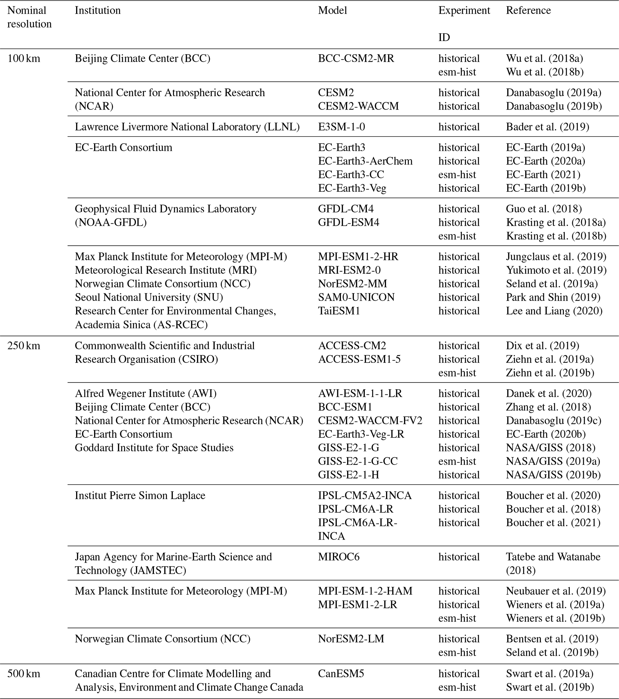
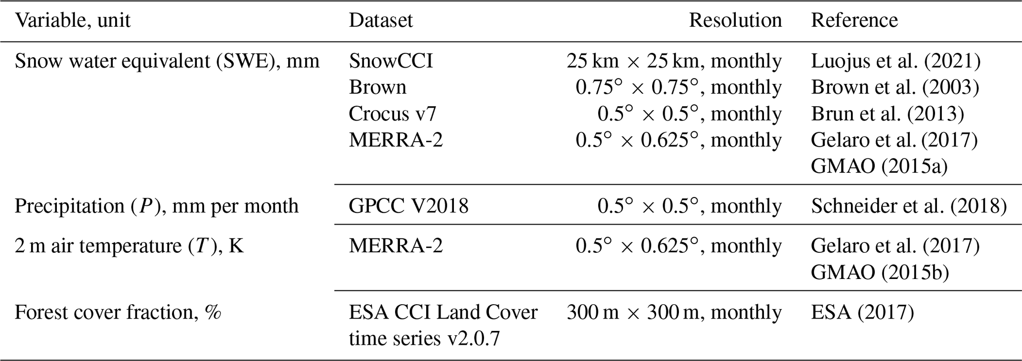
Table 2Observational and reanalysis datasets used in this study.
2.2 Observational and reanalysis data
For SWE reference data, we have used ESA CCI Snow “SnowCCI” (European Space Agency Climate Change Initiative, Snow) data for the non-mountainous regions and MERRA-2 (the Modern-Era Retrospective analysis for Research and Applications, Version 2; Gelaro et al., 2017; GMAO, 2015a), Brown (Brown et al., 2003), and Crocus v7 (Brun et al., 2013) data for the mountainous regions. SnowCCI data, which is the same product as the GlobSnow v3 SWE product (except provided in geographical latitude–longitude grid for easier comparison with climate model data), are based on satellite passive microwave radiometer data and in situ data (Luojus et al., 2021; Pulliainen et al., 2020). The SnowCCI algorithm combines microwave brightness temperature (Tb) data, observed by satellite instruments, with ground-based snow depth measurements from the global network of synoptic weather stations (Luojus et al., 2021). The SWE estimation algorithm is based on the difference in Tb between two frequencies (37 and 19 GHz). The ground beneath the snowpack emits microwaves, which propagate through the snowpack, being partially absorbed during the process. The low-frequency and high-frequency signals attenuate differently as they propagate through the snowpack, which makes the difference in Tb a good indicator for estimating SWE (Cagnati et al., 2004). The attenuation is affected by snow depth, snow grain size, and snow density. The high-frequency signal attenuates more than the low-frequency signal when it propagates through the snowpack, especially for a deep, dense, and large-grained snowpack. Thus, a large difference between high- and low-frequency signals indicates a high SWE (Kelly et al., 2003). The SnowCCI approach combines Tb differences with in situ snow depth observations, which considerably improves SWE estimation relative to a satellite-only retrieval (Pulliainen, 2006; Takala et al., 2011).
A recent bias-correction method combines the original SnowCCI data with extensive ground-based snow course SWE measurements, which significantly reduces the uncertainty of NH SWE estimation (Pulliainen et al., 2020). The method decreases the uncertainty of hemisphere-mean SWE estimation from 33 % to 7.4 %. The bias-corrected SnowCCI data are mapped to a 25 km EASE-Grid and are available from 1979. Mountainous regions, glaciers, and ice sheets are excluded from the data. The original SnowCCI data are available around the year, while bias-corrected SnowCCI data are only available from February to May. Despite limitations in its temporal coverage, we have used the bias-corrected data in this study. We chose to do this as the bias-correction method significantly reduced the uncertainty and made the observational data more accurate, which, in turn, makes the comparison with the models far more meaningful.
As the bias-corrected SnowCCI data are only available for non-mountainous grid cells, we have used an average of the MERRA-2, Brown, and Crocus v7 SWE products for the mountainous regions. MERRA-2 is a NASA (National Aeronautics and Space Administration) atmospheric reanalysis, and it is available from year 1980. The spatial resolution of the data is (Gelaro et al., 2017). From MERRA-2, we have used the SWE product (Gelaro et al., 2017; GMAO, 2015a). Brown SWE product, in turn, uses a simple snow scheme driven by ERA-Interim reanalysis (Brown et al., 2003). For the third SWE dataset, we have used Crocus version 7 product, which is a physical snow model driven by ERA-Interim reanalysis (Brun et al., 2013). Both MERRA-2 and Crocus v7 tend to slightly overestimate SWE under 150 kg m−2 and underestimate SWE over 150 kg m−2 (Mortimer et al., 2020).
For precipitation (P) and temperature (T) reference data, we used GPCC (Global Precipitation Climatology Centre) version 2018 precipitation data (Schneider et al., 2018) and MERRA-2 temperature data (Gelaro et al., 2017; GMAO, 2015b). GPCC is a monthly precipitation product based on data from rain gauge stations, and the data are available on a 0.5∘ global grid from 1891 to the present (Schneider et al., 2018). The product agrees well with other precipitation products (Behrangi et al., 2016; Sun et al., 2018). All precipitation data are presented here in units of kilograms per square meter per month (kg m−2 per month), which is equivalent to millimeters per month (mm per month).
For T reference data, we have used the monthly mean 2 m air temperature product, which agrees well with observations in the Arctic (Gelaro et al., 2017; Simmons et al., 2017), and the mean values show very small biases (Bosilovich et al., 2015). MERRA-2 daily temperature tends to have a cool daytime bias and a warm nighttime bias (Bosilovich et al., 2015; Draper et al., 2018). However, this is not a major issue for our study because we use the monthly mean product. In addition, MERRA-2 seems to underestimate global warming trends in the last years of our study period (Gelaro et al., 2017; Simmons et al., 2017). Additionally, we used the ESA CCI Land Cover time series v2.0.7 (ESA, 2017) to study the effect of forest cover on the results.
We used the nearest-neighbor method to resample CMIP6, Brown, Crocus v7, MERRA-2, and GPCC data to the 25 km equal-area projection. The fractional forest cover was calculated from the higher-resolution ESA CCI Land Cover time series as the fraction of forest cover grid cells of all cells within each 25 km × 25 km grid area. The bias-corrected SnowCCI data are available only for non-mountainous regions. Therefore, we used the bias-corrected SnowCCI data for the non-mountainous regions, and for the grid cells that were defined as mountainous in SnowCCI data, we used the mean SWE of the Brown, MERRA-2, and Crocus v7 datasets. The complex terrain causes uncertainties in SWE estimates, but averaging over multiple products can improve the accuracy (Mortimer et al., 2020). We calculated the model biases by subtracting the observation value from the model value, i.e., model minus observation, and compared the biases grid cell by grid cell. Our study covered land areas north of 40∘ N and years between 1982 and 2014. In this study, we mainly concentrated on snow-covered areas, i.e., grid cells where SWE >10 kg m−2. The snow-covered area was computed individually for each model and for each month. We have also filtered out grid cells with modeled SWE above 2000 kg m−2, as those values greatly exceed observed SWE (Stuefer et al., 2013).
We focus the analysis on two seasons: winter and spring. For the winter season, we consider only the SWE in February, since bias-corrected SnowCCI data are only available from February to May. We studied through linear regression analysis how the SWE bias in February depends on the precipitation (P) bias and temperature (T) biases, summed over the three preceding months from November to January:
where Pcum and Tcum are the precipitation and temperature summed over November–January, βP and βT are the regression coefficients, and C is the constant. Here, as well as in Eq. (2) below, Δ refers to the model bias, i.e., the difference between the modeled value (defined for each year separately) and the observed climatological value (averaged over the whole period considered). We used the climatological average for the observations because climate models cannot be expected to correctly simulate the weather conditions of individual years. Thus, the regression coefficients βP and βT depend only on the modeled interannual variations. The equations are presented in more detail in Appendix A.
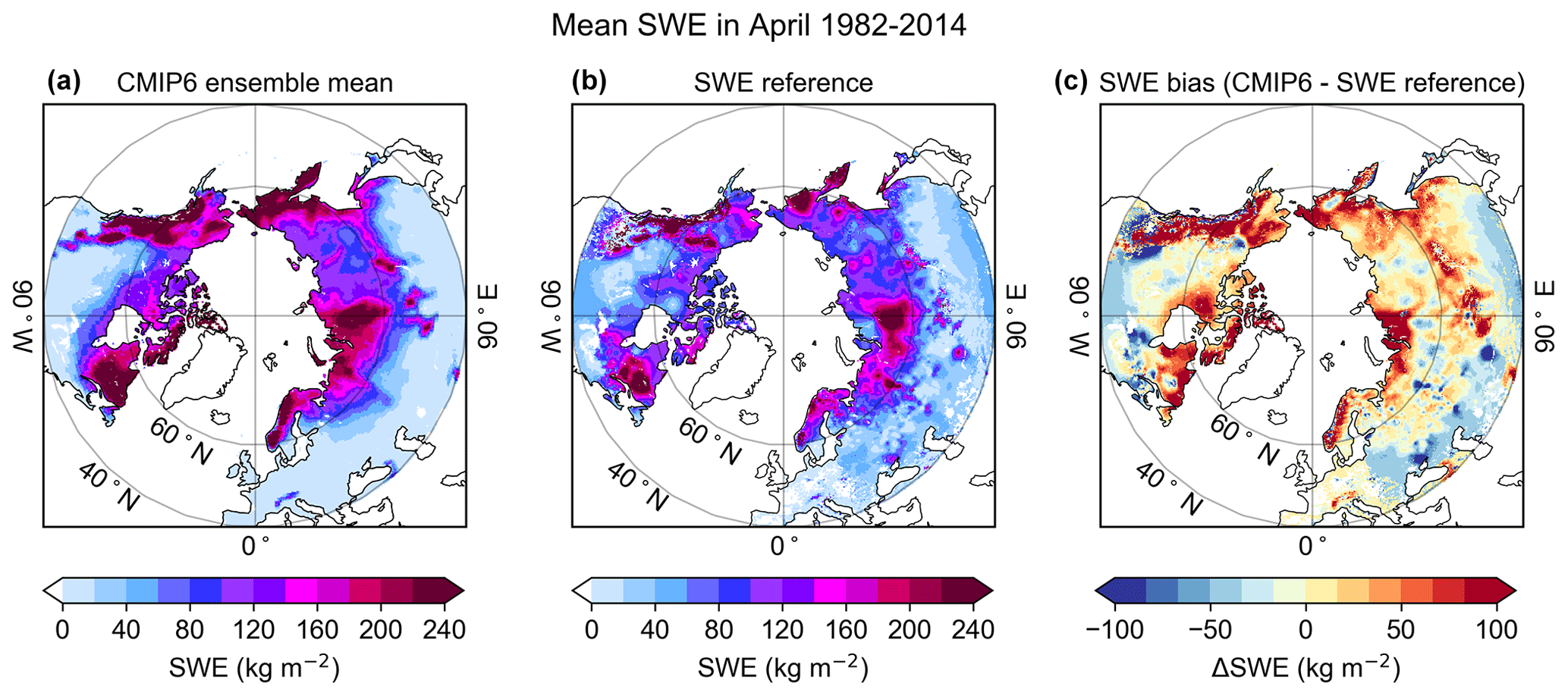
Figure 1Mean SWE in April for the CMIP6 high-resolution (100 km) multi-model ensemble mean (a), and the SWE reference data (b) and the model SWE bias (c) for the period 1982–2014.
For the spring season, we considered the monthly changes in SWE from February to March, from March to April, and from April to May. We defined the SWE change rate (SWEchange) as the difference in SWE between each month and the previous month. Positive values indicate an increase in SWE from one month to the next, and negative values indicate a decrease. The model-minus-observation difference ΔSWEchange (i.e., the model bias) was then regressed against the monthly precipitation and temperature biases:
For example, when considering SWEchange from February to March, we used P and T for March. We pooled together the values of ΔSWEchange, ΔP, and ΔT for the whole spring period (February through May) to determine the regression parameters βP and βT and C. The equations are presented in more detail in Appendix A.
We included only snow-covered grid cells (SWE >10 kg m−2) in the analysis and calculated the linear regressions only for grid cells with at least four values available during the study period. We calculated the linear regressions for the whole study period 1982–2014 and separately for three shorter periods: 1982–1991, 1992–2001, and 2002–2014.
By substituting into Eqs. (1) and (2) the mean model biases, it is possible to split the model SWE biases into three components: the contribution of P (PC), the contribution of T (TC), and the contribution of other factors. For SWE in winter, PC and TC are
Correspondingly, for SWEchange in spring, PC and TC are
The third component in both winter and spring is the residual term, which is the constant from the regression Eq. (1) or (2). This is the contribution of other factors, including, for example, inaccuracies in observational datasets and model parameterizations related to, for example, snow and surface energy budget. The residual (R) gives an estimate for the SWE bias that would remain if P and T were simulated correctly in the model.
Figure 1 shows as an example the mean SWE of all CMIP6 high-resolution (100 km) models, the mean of SWE reference data, and ΔSWE (CMIP6–SWE reference) in April during 1982–2014. The corresponding figures for precipitation and temperature are in the Supplement (Fig. S2). The SWE distribution has a large spatial variability: the highest values exceed 240 kg m−2 in both multi-model mean and SWE reference data, and these values are found in northeastern Canada, around the Rocky Mountains, in Scandinavia, and in some parts of Siberia. Although the SWE distribution is similar for the multi-model mean and SWE reference data, the models overestimate SWE in several regions, which are mostly located in the northern parts of the study area in northeastern Canada, northeastern Siberia, and Eurasia around 90∘ E. In the southern parts of the study area, the multi-model mean mainly underestimates SWE.
The monthly SWE sum of the whole study area varies considerably between the models (Fig. 2). In February, March, and April, the modeled SWEs (solid and dashed grey lines) vary by a factor of 2, and in May, they even vary by a factor of 3. The variability between models is notably larger than the uncertainty range of the SWE reference estimate (blue markers). The low-resolution models (thin grey lines) do not significantly differ from the high-resolution models (dashed lines); the SWE sum is mostly in the same range in both resolution groups. Also, the mean values for both high-resolution (red markers) and low-resolution (purple markers) models are very close to each other. However, there are two low-resolution models that show very high SWE sum values in every month, which are clear outliers. These outliers are “GISS-E2-1-G historical” and “GISS-E2-1-G-CC esm-hist”, and we have found that the anomalous values are due to a very high SWE in the mountainous areas. All models reach the highest SWE in March, which is consistent with observations. Overall, most models overestimate the monthly SWE sum, and the CMIP6 multi-model ensemble mean is higher than the SWE reference data in every month. While a few models underestimate the SWE sum especially in May, the majority of models overestimate the SWE sum in every month. We have performed the following detailed analysis only for the high-resolution models. In addition, since the results for the different model versions for each institute tend to be rather similar, only one model version for each of the 10 institutes is shown in the figures. Figures including all 17 high-resolution model versions are provided in the Supplement.
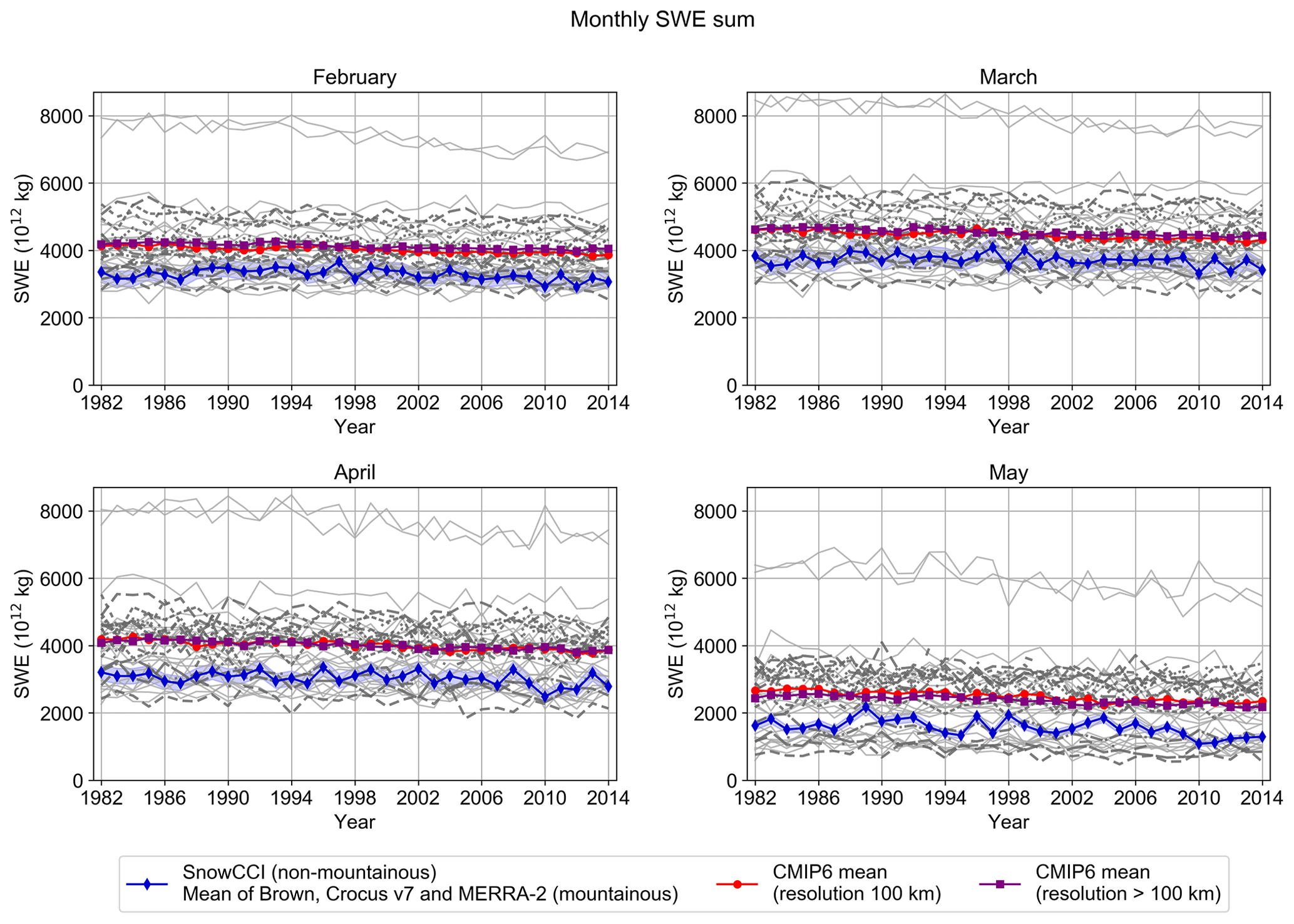
Figure 2Monthly SWE sum over the entire study area in February, March, April, and May separately for each high-resolution (100 km) CMIP6 model (grey dashed lines), for each low-resolution (>100 km) CMIP6 model (thin solid lines), for the high-resolution CMIP6 multi-model ensemble mean (red markers), for the low-resolution CMIP6 multi-model ensemble mean (purple markers), and for the SWE reference data (blue markers). The blue shaded area indicates the 7.4 % uncertainty range of the SWE reference data.
4.1 SWE in winter
The mean SWE bias in February shows large spatial variability within each model but also varies much between the models (Figs. 3 and S3). The areal-mean model bias varies from about −8 kg m−2 to 40 kg m−2. However, the largest negative and positive biases are well concentrated in the same areas in all models. Overall, the models tend to overestimate the SWE in the northern parts of the study area but also in southern Siberia. The negative biases, in turn, occur mostly in the south and especially on the coastal areas of North America. In some models, there are negative biases also in the middle parts of Eurasia. Large biases also occur over Rocky Mountains in every model, but the sign of the bias varies. The CESM2 and NorESM2-MM models show the largest overestimations. For both models, the bias is very high in large regions in northern parts of North America and Eurasia. In these areas the relative bias is typically 150 %–200 %. The BCC-CSM2-MR, E3SM-1-0, and SAM0-UNICON models also show large positive biases, which are concentrated in the same areas; although, the biases are clearly smaller than for the CESM2 and NorESM2-MM models. In other models, the areal-mean biases are closer to 0 kg m−2; however, regional differences exist. Overall, the GFDL models are the most consistent with the SWE reference data during February.
All models overestimate NH extratropical precipitation from November to January (Figs. 4 and S4). The largest overestimations are mainly in southern regions and in coastal areas. There are small areas where underestimation occurs, especially in Eurasia around 90∘ E. In every model, there are large regions where Pcum bias could logically explain the SWE bias (marked with dots), i.e., areas where models overestimate or underestimate both SWE and Pcum. These regions are mostly in the northern parts of the study area, whereas in the south there are more areas where SWE and Pcum discrepancies are more often not consistent with each other.
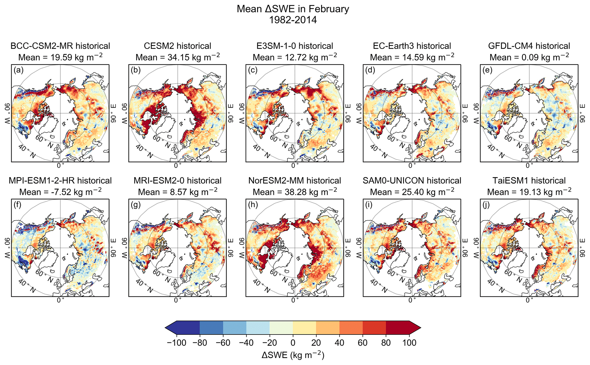
Figure 3The mean model bias in SWE (ΔSWE, model minus observation) in snow-covered areas in February 1982–2014.
For model T biases, the values are mostly positive; however, regional and intermodel variability exists (Figs. 5 and S5). We show ΔT (ΔTcum divided by 3) instead of ΔTcum so that the values are more intuitive and easier to interpret. The CESM2 and E3SM-1-0 models generally simulate too warm temperatures, and the largest positive biases are in the northern parts of the study area. The GFDL, MPI-ESM1-2-HR, and MRI-ESM2-0 models simulate too warm temperatures in the north, while the SAM0-UNICON and TaiESM1 models, in turn, simulate too cold temperatures in the north. The BCC-CSM2-MR and EC-Earth3 models are the most consistent with the MERRA-2 data. In every model, there are large areas where the signs of biases for T and SWE are opposite (marked with dots), indicating that biases in T might explain biases in SWE. However, in these areas, the biases are mainly quite small.
The contributions to SWE biases (ΔSWE) due to precipitation biases (PC), temperature biases (TC), and other factors (residual R) are quantified using the regression Eqs. (1), (3), and (4). To summarize their relative importance, Figs. 6 and S6 show the areal means of the absolute values of ΔSWE, PC, TC, and R. The mean ΔSWE varies from under 30 kg m−2 in the GFDL-CM4 model to around 50 kg m−2 in the CESM2 and NorESM2-MM models. In all models, the contribution of P on ΔSWE is clearly larger than the contribution of T. However, the residual is also typically large, indicating that P and T cannot explain the SWE biases alone. This implies that observational uncertainty or model structural factors, such as parameterizations related to the surface energy budget or hydrology, play a considerable part in the observed SWE biases. We studied the terms' statistical significance by using the t test and found that all the terms (PC, TC, and R) are significantly different from zero at the 99 % confidence level. The variability in these parameters between the decadal subperiods and the full three-decade analysis period was slight, indicating consistent behavior across time in both models and observations.
Figures 7 and S7 show the spatial distribution of the contributions of P and T and the residual for each model for the entire study period 1982–2014. The spatial distributions of R2, βP, and βT are shown in the Supplement (Fig. S8). Also, the contributions of P and T and the residual calculated for the shorter time periods are in the Supplement (Figs. S9–S11). Figure 7 shows that, overall, the contribution of P is larger than the contribution of T, as Fig. 6 already indicated. P contributes to ΔSWE especially over northern and coastal regions, with fairly similar patterns for all models considered. The regression coefficient βP also shows large values (βP≈1), especially in the northern and middle parts of both continents (Fig. S8), with relatively small intermodel variations. This is consistent with the expectation that in cold regions an increase in precipitation translates into a similar increase in SWE.
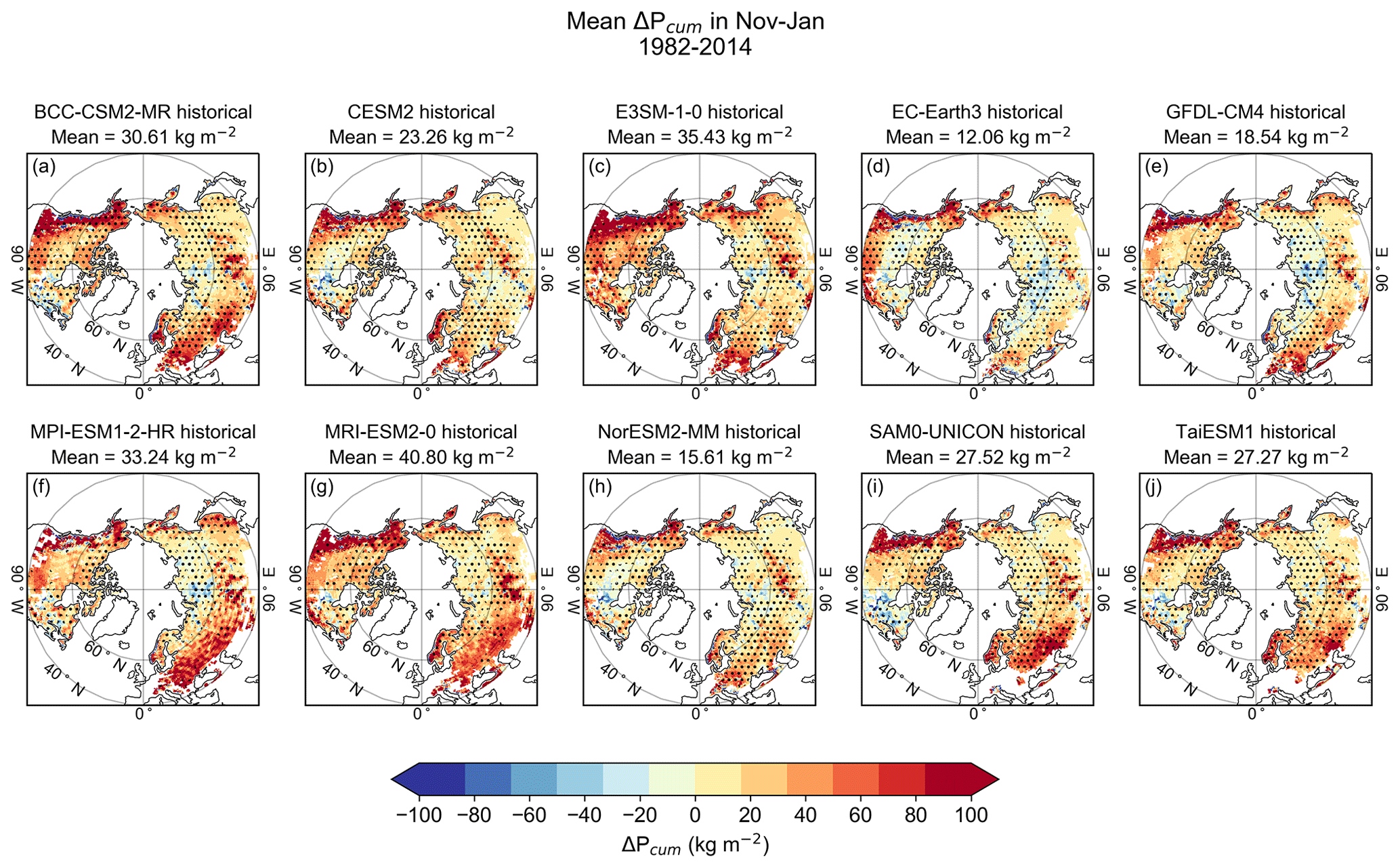
Figure 4The mean model bias in Pcum (ΔPcum, model minus observation) in snow-covered areas from November to January 1982–2014. The dots indicate areas where the models either overestimate both SWE and P or underestimate both SWE and P.
The contribution of T is mostly very weak (Fig. 7); however, for some models, T shows stronger contribution especially over western parts of Eurasia and over northeastern Canada. The regression coefficient βT is mostly negative or very close to zero (Fig. S8). The negative correlation is strongest in Europe and southern parts of North America and Eurasia. In these regions, the temperature is close to 0∘ C in winter, which makes temperature an important driver of the SWE. Northern Canada and Siberia, in turn, show areas with positive correlation, meaning that warmer temperatures cause higher SWE. Studies have shown that when the temperature rises due to climate change, the winter precipitation will also increase (Brown and Mote, 2009; Park et al., 2012; Räisänen, 2008). In the south, warming temperatures will shift winter precipitation from snow to rain. In the north, in turn, temperature will stay below 0∘ C despite the warming, which will lead to an increase in snowfall in the coldest regions of NH and, therefore, to an increase in SWE. This phenomenon is most likely seen here as well; warmer temperatures in the models will increase winter precipitation, resulting in too high SWE in the models. In fact, this exposes a limitation of the regression Eq. (1): it treats ΔTcum and ΔPcum as independent variables, which is not fully realistic. When these variables are correlated, their contributions to ΔSWE cannot be fully separated.
The residual shows large spatial and intermodel variability (Fig. 7). Especially for the CESM2 and NorESM2-MM models, the residual shows very large positive values. These large positive residuals are mainly concentrated in the same areas where the models clearly overestimate SWE (Fig. 3). This indicates that, for these models, the large SWE biases in these areas are mainly caused by some other factors than P or T. For other models, the residual shows both positive and negative values across the study area. The possible factors causing the large residual term are discussed in more detail in Sect. 5.2.
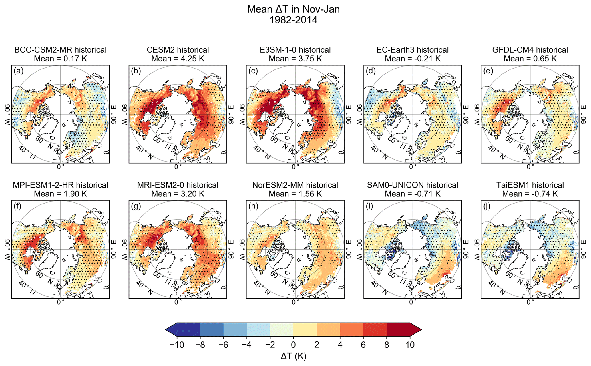
Figure 5The mean model bias in T (ΔT, model minus observation) in snow-covered areas from November to January 1982–2014. We show ΔT (ΔTcum divided by 3) instead of ΔTcum so that the values are more intuitive and easier to interpret. The dots indicate areas with either cold bias and positive SWE bias or warm bias and negative SWE bias, i.e., the areas where T bias could logically explain the SWE bias.
4.2 Monthly SWE change in spring
Figures 8 and S13 show the mean bias in monthly SWE change (ΔSWEchange) in spring in the snow-covered areas for the whole study period 1982–2014. A figure showing the SWE change rate of multi-model mean, SWE reference data, and bias in multi-model mean is in the Supplement (Fig. S12). Positive ΔSWEchange means that there is less snowmelt in the models compared to the SWE reference data, and negative ΔSWEchange indicates that snow melts faster in models, respectively. The areal-mean ΔSWEchange is mainly negative in every model, which means that snow melts generally faster in the models compared to the SWE reference data. However, there is a large spatial variability in every model, and the intermodel variability is also large. In the CESM2 and NorESM2-MM models, three areas show distinctly positive ΔSWEchange: northeastern Canada, northern Siberia, and eastern Siberia. In all these areas, the SWE bias in February (Fig. 3) was already clearly positive, meaning that these models greatly overestimate SWE in these areas also in spring. The EC-Earth3 model shows clear positive ΔSWEchange in northeastern Canada but also in Eurasia. The area with positive biases in Eurasia is very extensive and differs notably from the other models. The EC-Earth3 model has been found to drastically overestimate the snow cover extent as well (Mudryk et al., 2020). The SAM0-UNICON and TaiESM1 models also show positive values in northern Siberia. The GFDL and MPI-ESM1-2-HR models, in turn, show large areas with negative ΔSWEchange in northern Canada and in eastern parts of Siberia, which differs from the other models. Overall, the model biases in the SWE change rate in spring (Fig. 8) show larger intermodel variations than the corresponding biases in SWE in February (Fig. 3).
As in winter (Fig. 4), models on average overestimate precipitation in spring as well (Figs. 9 and S14). The largest overestimations occur mainly in southern regions and in coastal areas. The regions with mutual biases in P and SWEchange (marked with dots) show large intermodel variability, and they are less extensive than in winter (Fig. 4). This indicates that precipitation is not as important factor in spring as it is in winter.
The mean T bias in spring shows a large spatial variability within each model, but also the variability between models is very clear (Figs. 10 and S15). The BCC-CSM2-MR, E3SM-1-0, MPI-ESM1-2-HR, and MRI-ESM2-0 models show a warm bias in the northern parts of the study area, whereas the SAM0-UNICON and TaiESM1 models show a cold bias in the same area. The EC-Earth3 model, in turn, has a cold bias in eastern Eurasia near 60∘ N, which clearly differs from the other models. These areas also exhibited less snowmelt than the SWE reference data, which indicates that the bias in snow melt rate can be caused by the bias in T. The sizes and locations of the areas with mutually consistent biases in T and SWEchange (marked with dots) vary greatly between models. Especially in the GFDL-CM4 model, the size of these areas is small, while in most of the models, the dots cover the majority of the study area. Furthermore, in those regions where the biases in T and SWEchange are consistent in spring, the cold or warm temperature biases are typically relatively large, when compared with the corresponding biases in winter (Fig. 5). This indicates that biases in T are a more important driver of biases in SWE in spring than in winter.
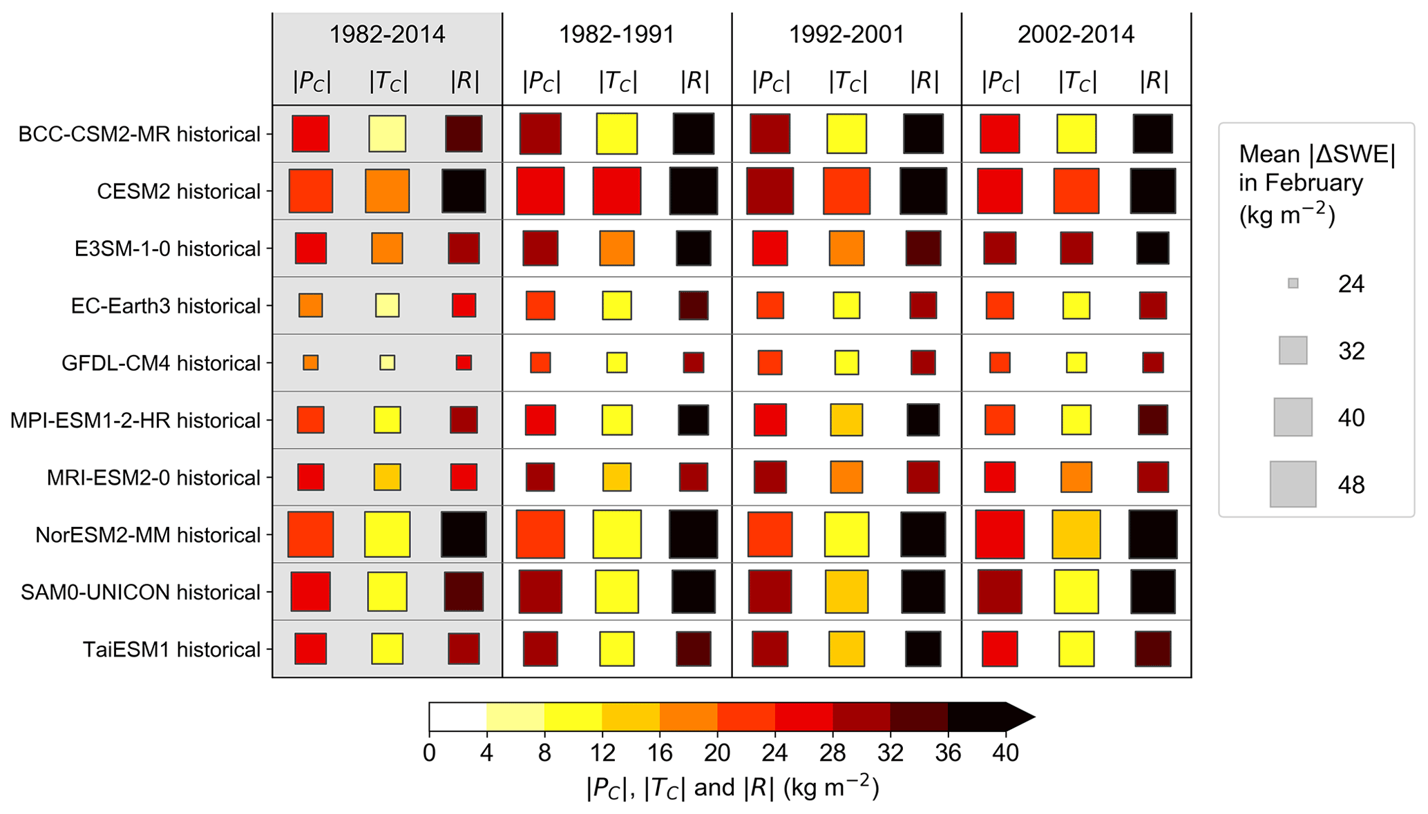
Figure 6The areal means of the absolute values of ΔSWE, PC, TC, and residual R calculated for the entire study period 1982–2014 (left column, shaded with grey) and for three shorter time periods (1982–1991, 1992–2001, and 2002–2014) for each model in winter. The size of the square indicates the absolute value of ΔSWE of that time period and model, and the color of the square indicates the absolute value of PC, TC, and R.
Figures 11 and S16 summarize the areal means of the absolute values of ΔSWEchange, the contribution of P (PC), the contribution of T (TC), and the contribution of other factors (the residual R). The contributions of P and T are quite similar in magnitude in almost all the models. None of the variables shows a large dependence on the period considered. The EC-Earth3 model stands out from the other models, as TC is larger than in the other models. The large contribution of T in ΔSWEchange was already seen in Figs. 8 and 10, as the spatial distribution of the biases were similar. This also suggests that the overestimated snow cover extent in the EC-Earth3 model (Mudryk et al., 2020) might be at least partly due to the cold bias. In all models, the residual is larger than PC or TC. This indicates that, overall, the biases in snow melt rate in spring are dominated by other factors than T or P. These factors will be further discussed in Sect. 5.2. We also studied the terms' statistical significance by using the t test. Even though the contributions of T and P are considerably smaller than the residual term, all the terms (PC, TC, and R) are significantly different from zero at the 99 % confidence level.
Figures 12 and S17 show the spatial distribution of the contributions of P and T and the residual for each model for the entire study period 1982–2014. The spatial distributions of R2, βP, and βT are displayed in the Supplement (Fig. S18). Also, the contributions of P and T and residual calculated for the shorter time periods are in the Supplement (Figs. S19–S21). P contributes to ΔSWEchange mostly in Alaska and northern Siberia, but the effect varies between models. Furthermore, even though T showed clear warm and cold biases in many areas (Fig. 10), the contribution of T is mostly quite weak, because of the small regression coefficient βT (Fig. S6). However, exceptions exist; in particular, the EC-Earth3 and EC-Earth3-Veg models stand out, as in Eurasia there is a large area where a negative bias in T (Fig. 10) contributes substantially to a positive bias in SWEchange (Fig. 8). Also, for the CESM2 and GFDL-ESM4 models, T shows a stronger contribution over northern parts of North America. Overall, however, the contributions of both P and T are small compared to the residual R, which is consistent with Fig. 11. This indicates that other factors than T or P are the dominant drivers for the SWEchange discrepancies. The residual is mostly negative in all the models, which means that snow would melt too fast in the models if T and P were simulated correctly. This issue is discussed further in Sect. 5.2.
The analysis shows that CMIP6 models overestimate the total SWE mass over the entire study area with a few exceptions (Fig. 2), which is consistent with the previous study (Mudryk et al., 2020). The overestimation of SWE was also observed in CMIP5 models (Mudryk et al., 2020; Santolaria-Otín and Zolina, 2020). The NH SWE sum reaches its peak value in March, but the peak values are overestimated by most of the models. As the spring advances, the variability between models increases, and some of the models clearly overestimate the SWE in May. In some models, in turn, snow melts faster than in the observations, and they underestimate SWE in late spring. This is also shown in Figs. 3 and 8: in winter, the SWE biases are mainly positive (Fig. 3), while in spring there are large differences in snow melt rates between the models (Fig. 8).
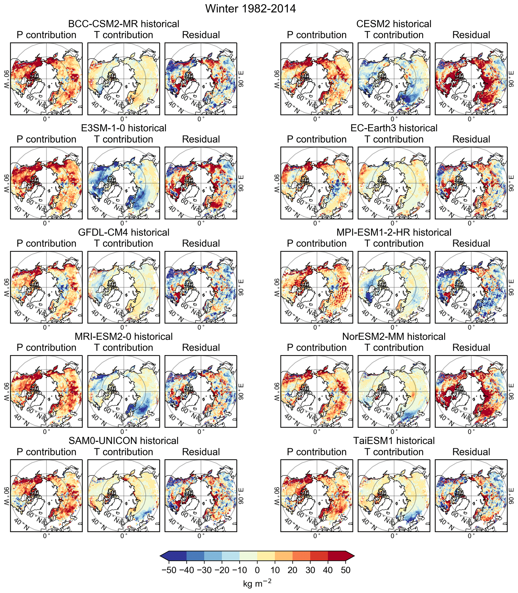
Figure 7Spatial distribution of the P contribution, the T contribution, and the residual for each model in winter 1982–2014.
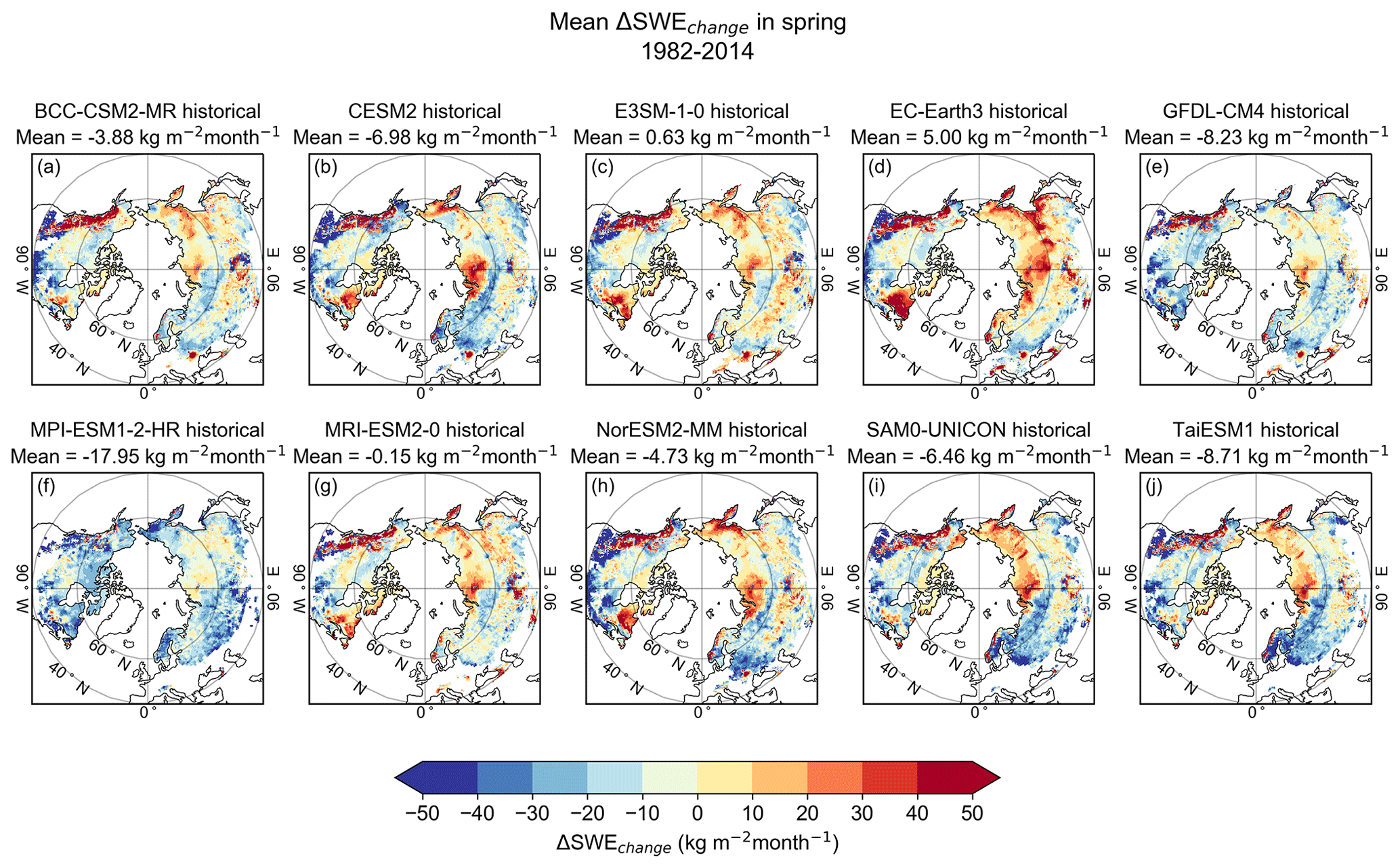
Figure 8The mean model bias in the monthly SWE change (ΔSWEchange, model minus observation) in spring for the period 1982–2014.
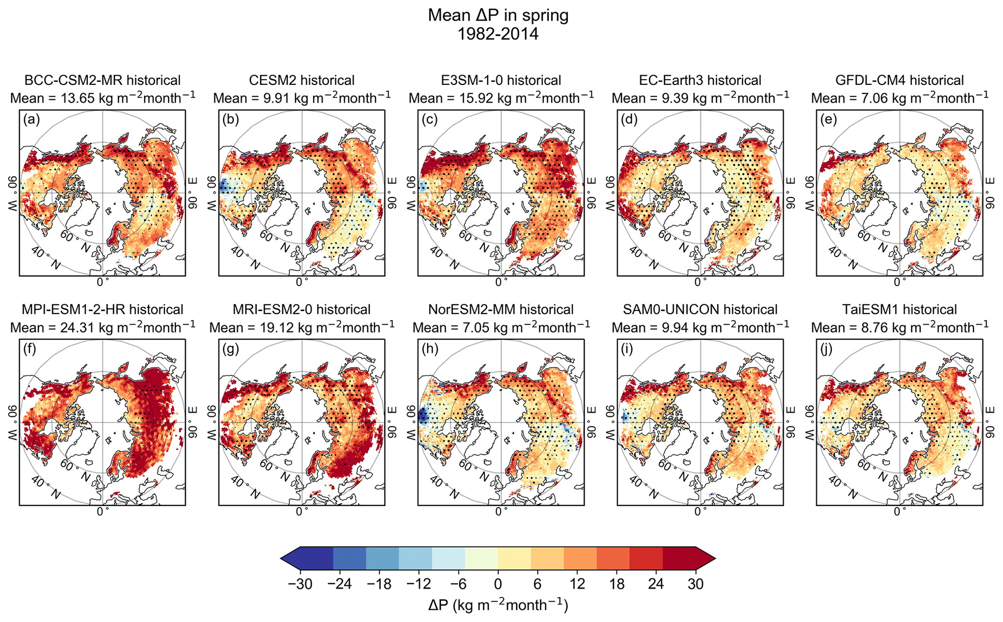
Figure 9The mean model bias in P (ΔP, model minus observation) in snow-covered areas in spring 1982–2014. The dots indicate areas where models either overestimate both SWEchange and P or underestimate both SWEchange and P.
5.1 The contribution of P and T to the SWE bias
In winter, the models mostly overestimate SWE (Fig. 3), but spatial and intermodel variability exists. The overestimations are mostly concentrated in the same areas in all models, but the magnitude varies greatly between the models. The models also overestimate precipitation in winter (Fig. 4), suggesting that overestimated SWE is caused by the overestimated P. The regression coefficient βP also shows very clear correlation between ΔSWE and ΔPcum (Fig. S8). Therefore, P clearly contributes to the SWE bias, whereas the contribution of T is substantially smaller (Fig. 7). This result is consistent with the expectation that precipitation is needed to initiate the snow cover. In other words, even too cold temperatures cannot cause too high SWE without precipitation. Also, studies have shown that both the P bias (Zamani et al., 2020) and the SWE bias (Mudryk et al., 2020) have decreased from CMIP5 to CMIP6. This indicates that there is a connection between these variables, which is consistent with the results from this study.
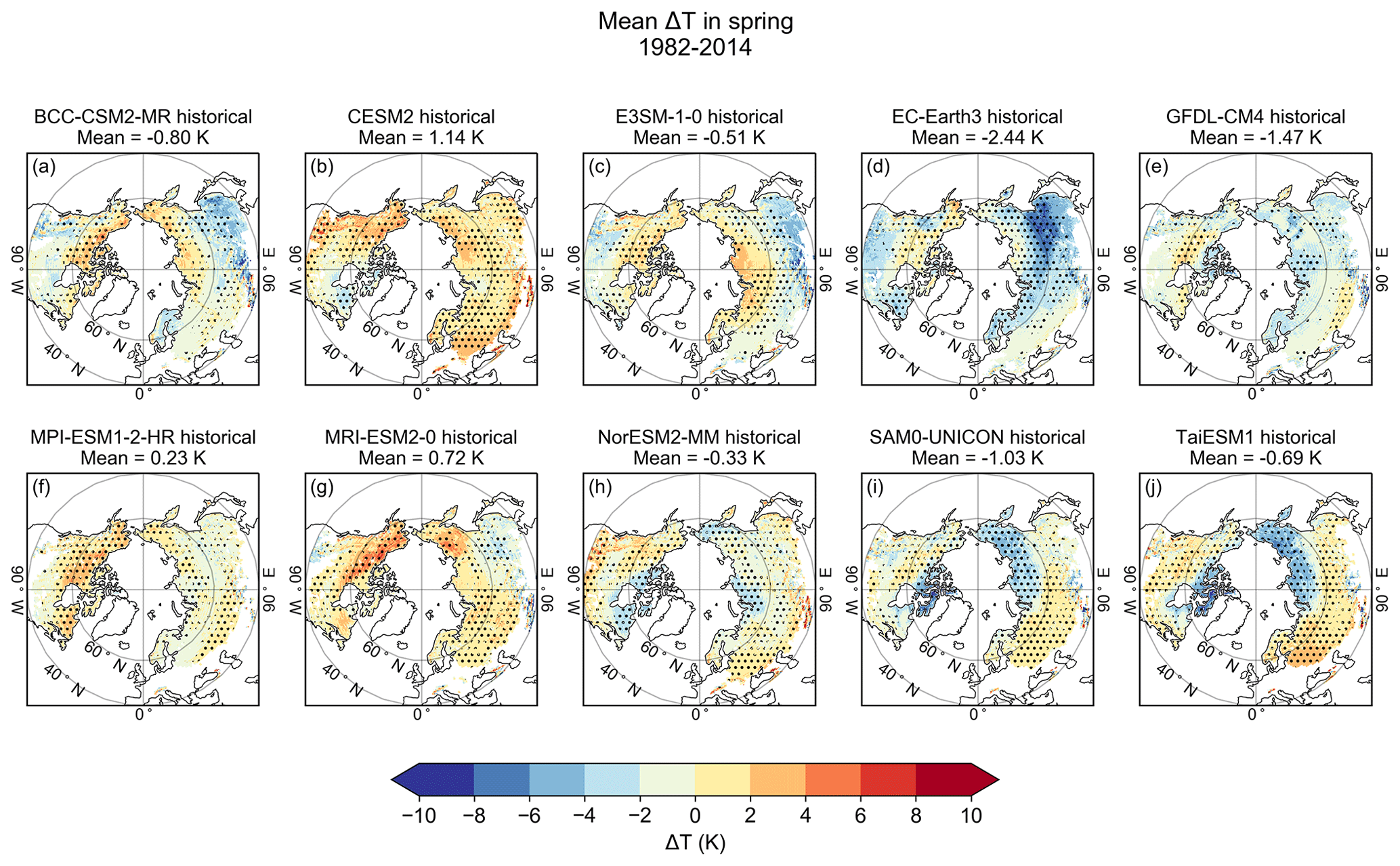
Figure 10The mean model bias in T (ΔT, model minus observation) in snow-covered areas in spring 1982–2014. The dots indicate areas with either cold bias and positive SWE bias or warm bias and negative SWE bias, i.e., the areas where T bias could logically explain the SWE bias.
The link between ΔTcum and ΔSWE is strongest in the warmest regions of the study area (Figs. 7 and S8). Especially in the coldest regions, where T is well below 0∘ C, variations in T do not significantly affect the amount of snow on the ground. In regions where T is closer to 0∘ C in winter, T plays a more significant role and has a greater impact on SWE. This physically reasonable behavior suggests that climate models might be able to simulate SWE trends in the warming climate correctly, even if SWE itself is not reproduced accurately.
In spring, ΔSWEchange and ΔT show quite similar patterns in many models (Figs. 8 and 10), which indicates that biases in T affect the biases in SWEchange. This result is to be expected because the increase in T is the main factor that causes snow to melt in spring. A relationship between temperature and snow cover in spring has also been observed in CMIP5 models (Brutel-Vuilmet et al., 2013; Mudryk et al., 2017). The CMIP5 models have been found to underestimate the observed trend towards a reduced snow cover extent due to an underestimation of the spring warming trend (Brutel-Vuilmet et al., 2013).
Even though ΔSWEchange and ΔT are quite consistent with each other, the contribution of T is not very strong (Fig. 12), because the regression coefficient βT is small (Fig. S18). The only model showing clear contribution of T is EC-Earth3, as there is a large area in eastern Eurasia where positive values of ΔSWEchange co-occur with a cold bias. The spatial distribution of the bias in SWEchange in the EC-Earth3 model differs considerably from other models (Fig. 8). The model has been found to drastically overestimate snow cover extent though not so much the SWE (Mudryk et. al. 2020). This suggests that while the positive bias in SWEchange (i.e., underestimated snowmelt rate in spring) is related to the cold bias, the cold bias might be maintained by a too high surface albedo resulting from overestimated snow cover extent.
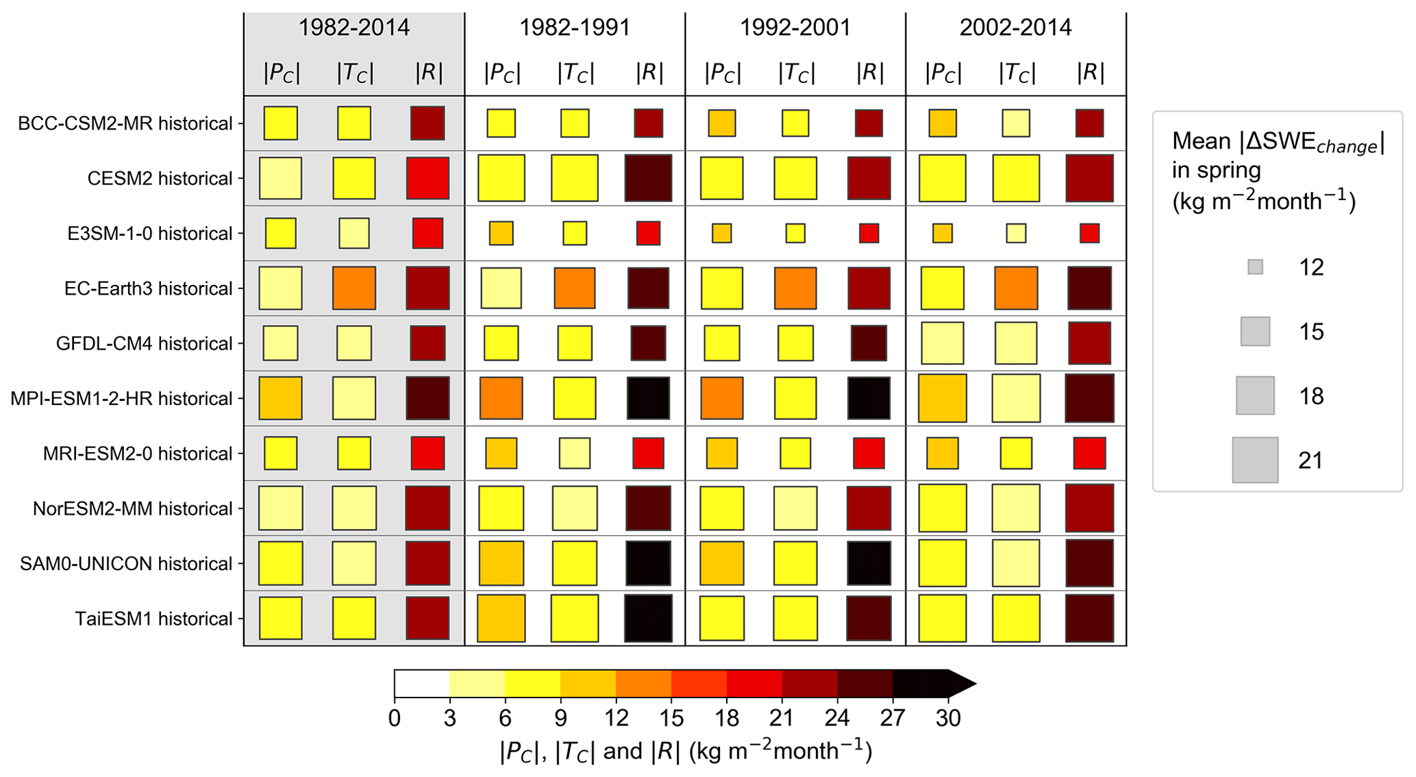
Figure 11The areal means of absolute values of ΔSWEchange, PC, TC, and residual R calculated for the entire study period 1982–2014 (left column, shaded with grey) and for three shorter time periods (1982–1991, 1992–2001, and 2002–2014) for each model in spring. The size of the square indicates the mean absolute value of ΔSWEchange of that time period and model, and the color of the square indicates the mean absolute value of PC, TC, and R.
Several factors can weaken the regression coefficient βT. The analysis shows that in spring the relationship between ΔT and ΔSWEchange is strongest in western parts of Eurasia and in southern parts of North America (Fig. S18). These are regions with the earliest snowmelt onset. In these areas, T is the dominant factor causing snow to melt throughout the spring season. In the northernmost parts of the study area, the melt season begins later, so that early spring still belongs to the snow accumulation season. As a result, P may still be the dominant factor influencing ΔSWEchange in early spring, and T will become a more significant factor later in the spring. This can reduce the correlation and affect R2, βP, and βT in the northern parts of the study area. Additionally, if SWE in winter is simulated incorrectly, this can affect the melt rates in spring, as there can be too little or too much snow that can melt.
5.2 The residual term
In both winter and spring, the residual term R of the regressions is also significant (Figs. 6, 7, 11, and 12). This means that the model biases in SWE in winter and SWEchange in spring cannot be entirely explained by the biases in P and T, but other factors also contribute to these biases. These factors may include inaccuracy in the model parameterizations related to snow and surface energy budget but also inaccuracy in the observational datasets.
The residual term R is particularly pronounced for the SWE change rate in spring, when it is typically larger than either the contribution of P or T. Interestingly, the residual is mostly negative (Fig. 12). The negative residual means that if P and T were simulated correctly in the models, snow would melt too fast in spring. While understanding the origins of this bias would be worth a separate study, a previous study with ECHAM5 (Räisänen et al., 2014) is of interest here. ECHAM5 is a predecessor of the atmospheric part of MPI-ESM1-2-HR, for which the residual R in Fig. 12 is especially strongly negative. This is consistent with the finding that in ECHAM5 snow melted generally too fast in spring, despite a cold bias in T (Räisänen et al., 2014). A major factor for this was that T was not calculated separately for snow-covered and snow-free parts of the grid cell. Because of that, T was not able to rise above 0∘ C if there was snow left in the grid cell, and, therefore, a too large fraction of the available energy was used in melting the snow (Räisänen et al., 2014).
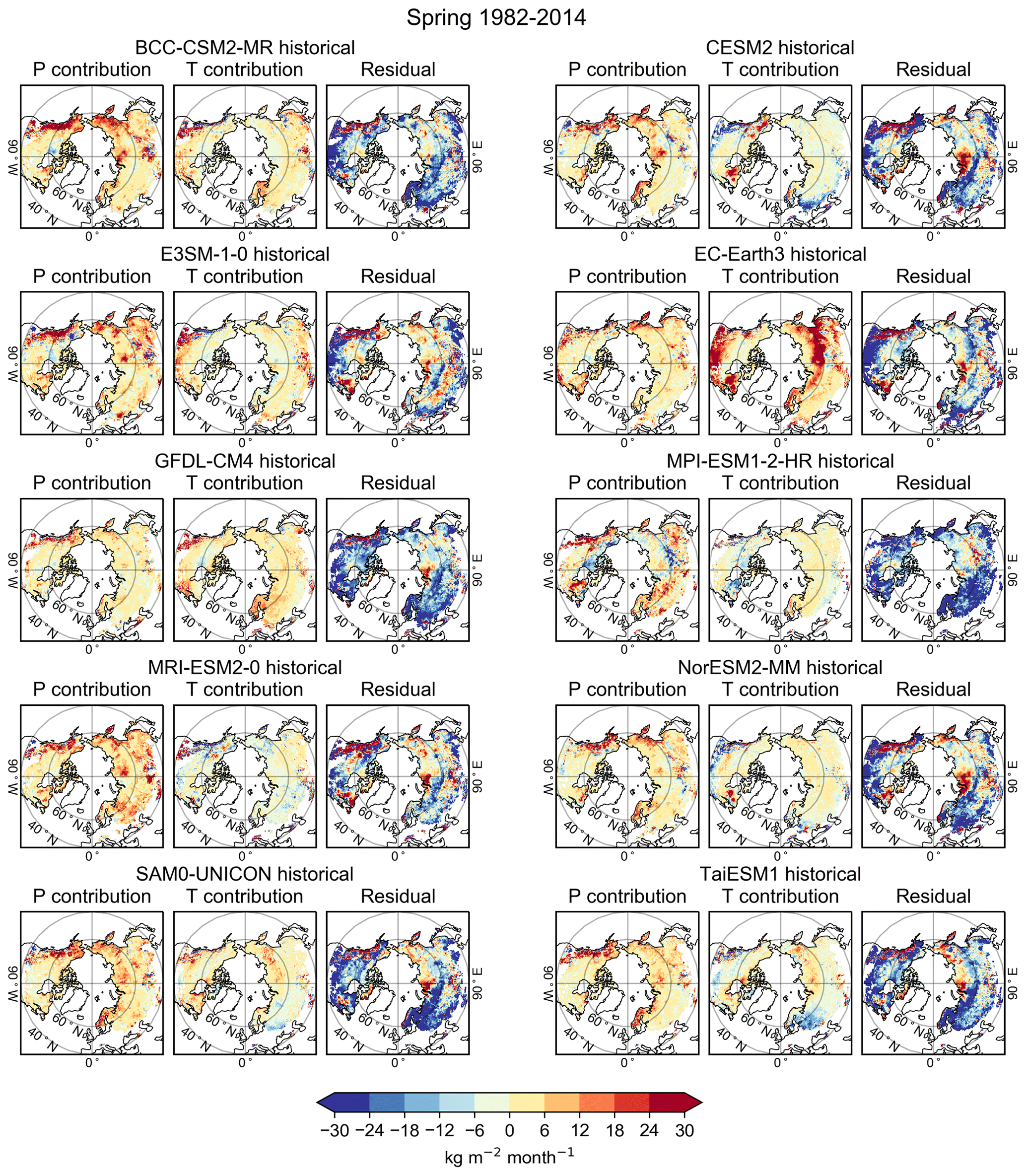
Figure 12Spatial distribution of the P contribution, the T contribution, and the residual for each model in spring 1982–2014.
The parameterization of the surface albedo is another factor that influences the snowmelt rate. In spring, the surface albedo feedback is strong, and if the albedo is not correctly simulated in the models, it can cause large biases in SWE in spring (Thackeray et al., 2018). CMIP5 models have had challenges in simulating correctly the surface albedo on snow-covered land (Thackeray et al., 2015). The intermodel variability in surface albedo feedback is large in CMIP5 models (Qu and Hall, 2014; Thackeray et al., 2018), and the large variability has been found to persist in CMIP6 models (Thackeray et al., 2021), suggesting that there are still large uncertainties in simulating the surface albedo. Specifically, regarding the discussion on ECHAM5 and MPI-ESM1-2-HR above, the only region in which MPI-ESM1-2-HR displays a positive residual in Fig. 12 is southeastern Siberia. In this very region, ECHAM5 featured delayed snowmelt, related to overly high albedo in the presence of vegetation over snow (Räisänen et al., 2014). While the specific mechanisms leading to too fast snowmelt might differ in different models, the example of ECHAM5 highlights the importance of the treatment of the surface energy budget in the presence of snow.
In addition to issues related to the models, uncertainties in the observational data can also affect the residual values. With the bias-correction method, SWE data are more accurate than before, but the uncertainty in hemisphere-mean values is still 7.4 %. In mountainous regions, the complex terrain poses a challenge in the SWE estimation, but averaging over multiple products can improve the accuracy (Mortimer et al., 2020). There are also uncertainties associated with the GPCC and MERRA-2 datasets that can cause errors in assessing the model biases; for example, MERRA-2 underestimates global warming trends in the last years of our study period compared to other reanalyses (Gelaro et al., 2017; Simmons et al., 2017). Snow cover in spring is especially sensitive to warming (Hernández-Henríquez et al., 2015), and, therefore, the uncertainties in MERRA-2 can affect the results especially in spring.
The uncertainties associated with the GPCC precipitation product can be divided into two categories: the systematic measuring error and stochastic sampling error (Schneider et al., 2014). The systematic error results from evaporation and from droplets and snowflakes being drifted across the gauge funnel. This error almost always causes underestimation of precipitation (Schneider et al., 2014). The sampling error, in turn, is caused by the sparse network density of the in situ stations, and the error increases when the density of the network decreases. A correction method taking into account the weather conditions has been implemented in the GPCC to improve the P estimate (Schneider et al., 2014). In general, estimating precipitation in high latitudes is a challenge. The estimates have improved, but especially regional discrepancies still exist between different precipitation products (Behrangi et al., 2016). This causes uncertainties in assessing the model bias and means that the choice of the precipitation product may influence the results.
We additionally studied the dependency between the residual term and fractional forest cover (Fig. S22), and we did this separately for the entire study area and for non-mountainous regions. In the entire study area, the spread of the residual term is quite large when the fraction of forest cover is small in both winter and spring. When looking at only the non-mountainous areas, the spread decreases compared to the entire study area, especially in spring. This illustrates that the residual term is particularly large in mountainous areas, indicating that in mountainous areas, T or P can only explain a small fraction of SWE bias, but other factors contribute SWE bias considerably. Also, in mountainous areas, the intermodel variability of the residual term is substantial. The complex terrain and large SWE variability make SWE estimates challenging. Also, the original resolution of CMIP6 models can be too coarse for accurately describing SWE in mountainous terrain; biases in snow cover and snow depth have been found to decrease considerably with downscaled regional climate models in mountainous regions (Matiu et al., 2019). Resampling the datasets to a common grid can cause uncertainties in mountainous areas due to the high topographic variability within a grid cell.
For most models, the residual term in non-mountainous areas in winter depends little on the fractional forest cover, indicating that the residual arises from other sources. For the CESM2 and NorESM2-MM models, however, the residual decreases when forest cover fraction increases, and this dependency is strikingly similar for these two models. Since CESM2 and NorESM2-MM both employ the CLM5 land surface model (Lawrence et al., 2019), this hints that the large positive SWE residual in these models originates from CLM5. Also, a unique feature within CESM2 that may cause high residual values in the coldest regions is that the model allows for a very large maximum SWE to enable the simulation of firn production over ice sheets (van Kampenhout et al., 2017). Even though our study does not cover ice sheets, this feature may cause positive SWE bias in the coldest regions of the study area (e.g., in the northernmost regions of Canada).
In spring in non-mountainous areas, the residual of SWEchange depends quasi-systematically on the forest cover fraction. While the level of the residual terms varies between the models, the values increase with increasing forest cover fraction in all models. The residual varies mostly between −25 and −12 kg m−2 per month for open areas and between −13 and −2 kg m−2 per month when the forest cover fraction is close to 100 %. This leaves room for at least two possible interpretations. On one hand, the larger intermodel spread of the residual over open areas suggests that problems in snow albedo parameterization (e.g., how to account for snow metamorphism, Colbeck, 1982) could be at least partly responsible for the large residual term. Due to the shading effect of the canopy (Malle et al., 2019), snow albedo treatment differences in the models should manifest more strongly over open tundra regions and less so over dense forest cover. On the other hand, the quasi-systematic dependence of the residual on the forest cover fraction could also point to some subtle issues in the SWE estimates of the SnowCCI dataset in spring.
Overall, the reasons behind the residual term are complex, and more detailed model-specific investigations for all participating CMIP6 models are beyond the scope of this study. Further analysis would be required in the future to fully understand the factors behind the residual term.
We have intercompared NH SWE estimates between CMIP6 models and observation-based SWE reference data and studied whether model biases in precipitation (P) or temperature (T) could explain the SWE model biases. Our study covered land areas north of 40∘ N and years between 1982 and 2014. We analyzed separately the SWE in winter (in February) and the SWE change rate in spring (SWEchange from February to May). Using regression analysis, we divided the SWE model bias (ΔSWE and ΔSWEchange, model minus observation) into three components: the contribution of P, the contribution of T, and the contribution of other factors, such as deficiencies in model parameterizations or inaccuracies in the observational datasets. The main findings in our study are as follows.
-
The models generally overestimate SWE, but large variability exists between models. The largest overestimations occur mainly in the northernmost parts of both Eurasia and North America. In winter, the overestimated SWE is mainly concentrated in the same areas in every model, but the magnitude differs between the models. In spring, the snow melt rates vary clearly between the models.
-
In winter, the SWE biases can be explained mostly with the P biases. The contribution of T is clearly smaller than that of P. This is in line with the expected results, as even too cold temperatures cannot cause too high SWE without precipitation. However, other factors contribute to SWE discrepancies as well.
-
In spring, T and P explain partly the biases in SWEchange. Especially cold or warm biases often co-occur with large SWEchange biases, but large spatial and intermodel variability exists. The importance of T in explaining SWEchange discrepancies during spring is to be expected, because the increase in T is the main factor that causes snow to melt as spring progresses. Yet it should be noted that the contribution of other factors, such as observation uncertainty or deficiencies in model parameterizations, is more significant in spring than in winter.
Overall, the study showed that the models still need to be improved to accurately describe SWE. However, the analysis also showed that there is a link between T and SWE, especially in the warmer regions of the study area, suggesting that climate models may be able to simulate SWE trends in a warming climate correctly, even if SWE itself is not accurately reproduced. Uncertainties in the observational data also cause uncertainties in the analysis, so by improving the observational data, we can study the models' ability to describe the snow cover more reliably and, thus, further improve the models.
The steps for calculating the model biases in SWE, T, and P and subsequently the linear regressions in winter are as follows.
-
We calculated cumulative T (Tcum) and P (Pcum) from November to January for each model and for the observational datasets:
-
We calculated the model bias in cumulative T (ΔTcum) and P (ΔPcum):
-
We calculated the model bias in SWE (ΔSWE) in February:
-
We calculated the linear regression for the biases using the ordinary least squares method:
where βT and βP are the regression coefficients, and C is the constant.
The steps for calculating the biases in SWEchange, T, and P and subsequently the linear regressions in spring are as follows.
-
We calculated monthly change in SWE (SWEchange) for each model and for the SWE reference data:
-
We calculated the model biases in monthly SWEchange (ΔSWEchange):
-
We calculated the model biases in T (ΔT) and P (ΔP) in March, April, and May:
-
We pooled together the values of ΔSWEchange, ΔP, and ΔT for the whole spring period (February through May) and calculated the linear regression for the biases using the ordinary least squares method:
where βT and βP are the regression coefficients, and C is the constant.
The CMIP6 model data are available at the Earth System Grid Federation (https://esgf-node.llnl.gov/search/cmip6/, ESGF, 2021). The bias-corrected SnowCCI data are available online at https://doi.org/10.1594/PANGAEA.911944 (Luojus et al., 2020). The Brown and Crocus v7 datasets are available from the original authors (please see Table 2 for references). MERRA-2 SWE data are available online at https://doi.org/10.5067/RKPHT8KC1Y1T (GMAO, 2015a). The original SnowCCI data and the ESA CCI Land Cover time series v2.0.7 are available at the ESA CCI data portal (https://climate.esa.int/en/odp/) (ESA, 2022). The MERRA-2 temperature data are available at https://doi.org/10.5067/AP1B0BA5PD2K (GMAO, 2015b). The GPCC data are available at the DWD website (https://doi.org/10.5676/DWD_GPCC/FD_M_V2018_050) (Schneider et al., 2018).
The supplement related to this article is available online at: https://doi.org/10.5194/tc-16-1007-2022-supplement.
KK performed the analysis and produced the figures with substantial contributions from AR and PR. KL provided the SWE reference data. AL contributed to collecting the CMIP6 model data. KK wrote the original draft. All authors contributed to manuscript review and editing.
The contact author has declared that neither they nor their co-authors have any competing interests.
Publisher’s note: Copernicus Publications remains neutral with regard to jurisdictional claims in published maps and institutional affiliations.
The authors would like to thank the two anonymous referees for their constructive comments.
This research has been supported by the Academy of Finland (grant no. 309125).
This paper was edited by Carrie Vuyovich and reviewed by two anonymous referees.
Bader, D. C., Leung, R., Taylor, M., and McCoy, R. B.: E3SM-Project E3SM1.0 model output prepared for CMIP6 CMIP historical, Earth System Grid Federation [data set], https://doi.org/10.22033/ESGF/CMIP6.4497, 2019.
Barnett, T., Adam, J., and Lettenmaier, D.: Potential impacts of a warming climate on water availability in snow-dominated regions, Nature, 438, 303–309, https://doi.org/10.1038/nature04141, 2005.
Behrangi, A., Christensen, M., Richardson, M., Lebsock, M., Stephens, G., Huffman, G. J., Bolvin, D., Adler, R. F., Gardner, A., Lambrigtsen, B., and Fetzer, E.: Status of high-latitude precipitation estimates from observations and reanalyses, J. Geophys. Res.-Atmos., 121, 4468–4486, https://doi.org/10.1002/2015JD024546, 2016.
Bentsen, M., Oliviè, D. J. L., Seland, Ø., Toniazzo, T., Gjermundsen, A., Graff, L. S., Debernard, J. B., Gupta, A. K., He, Y., Kirkevåg, A., Schwinger, J., Tjiputra, J., Aas, K. S., Bethke, I., Fan, Y., Griesfeller, J., Grini, A., Guo, C., Ilicak, M., Karset, I. H. H., Landgren, O. A., Liakka, J., Moseid, K. O., Nummelin, A., Spensberger, C., Tang, H., Zhang, Z., Heinze, C., Iversen, T., and Schulz, M.: NCC NorESM2-MM model output prepared for CMIP6 CMIP historical, Earth System Grid Federation [data set], https://doi.org/10.22033/ESGF/CMIP6.8040, 2019.
Bormann, K. J., Brown, R. D., Derksen, C., and Painter, T. H.: Estimating snow-cover trends from space, Nat. Clim. Change, 8, 924–928. https://doi.org/10.1038/s41558-018-0318-3, 2018.
Bosilovich, M. G., Akella, S., Coy, L., Cullather, R., Draper, C., Gelaro, R., Kovach, R., Liu, Q., Molod, A., Norris, P., Wargan, K., Chao, W., Reichle, R., Takacs, L., Vikhliaev, Y., Bloom, S., Collow, A., Firth, S., Labow, G., Partyka, G., Pawson, S., Reale, O., Schubert, S. D., and Suarez, M.: MERRA-2: Initial evaluation of the climate, Technical Report Series on Global Modeling and Data Assimilation, Vol. 43, edited by: Koster, R. D., National Aeronautics and Space Administration, Maryland, USA, 145 pp., 2015.
Boucher, O., Denvil, S., Levavasseur, G., Cozic, A., Caubel, A., Foujols, M.-A., Meurdesoif, Y., Cadule, P., Devilliers, M., Ghattas, J., Lebas, N., Lurton, T., Mellul, L., Musat, I., Mignot, J., and Cheruy, F.: IPSL IPSL-CM6A-LR model output prepared for CMIP6 CMIP historical, Earth System Grid Federation [data set], https://doi.org/10.22033/ESGF/CMIP6.5195, 2018.
Boucher, O., Denvil, S., Levavasseur, G., Cozic, A., Caubel, A., Foujols, M.-A., Meurdesoif, Y., Balkanski, Y., Checa-Garcia, R., Hauglustaine, D., Bekki, S., and Marchand, M.: IPSL IPSL-CM5A2-INCA model output prepared for CMIP6 CMIP historical, Earth System Grid Federation [data set], https://doi.org/10.22033/ESGF/CMIP6.13661, 2020.
Boucher, O., Denvil, S., Levavasseur, G., Cozic, A., Caubel, A., Foujols, M.-A., Meurdesoif, Y., Balkanski, Y., Checa-Garcia, R., Hauglustaine, D., Bekki, S., and Marchand, M.: IPSL IPSL-CM6A-LR-INCA model output prepared for CMIP6 CMIP historical, Earth System Grid Federation [data set], https://doi.org/10.22033/ESGF/CMIP6.13601, 2021.
Brown, R. D. and Mote, P. W.: The response of Northern Hemisphere snow cover to a changing climate, J. Climate, 22, 2124–2145, https://doi.org/10.1175/2008JCLI2665.1, 2009.
Brown, R. D., Brasnett, B., and Robinson, D.: Gridded North American monthly snow depth and snow water equivalent for GCM evaluation, Atmos.-Ocean, 41, 1–14, https://doi.org/10.3137/ao.410101, 2003.
Brun, E., Vionnet, V., Boone, A., Decharme, B., Peings, Y., Vallette, R., Karbou, F., and Morin, S.: Simulation of northern Eurasian local snow depth, mass, and density using a detailed snowpack model and meteorological reanalyses, J. Hydrometeorol., 14, 203–219, https://doi.org/10.1175/JHM-D-12-012.1, 2013.
Brutel-Vuilmet, C., Ménégoz, M., and Krinner, G.: An analysis of present and future seasonal Northern Hemisphere land snow cover simulated by CMIP5 coupled climate models, The Cryosphere, 7, 67–80, https://doi.org/10.5194/tc-7-67-2013, 2013.
Cagnati, A., Crepaz, A., Macelloni, G., Pampaloni, P., Ranzi, R., Tedesco, M., Tomirotti, M., and Valt, M.: Study of the snow melt–freeze cycle using multisensory data and snow modeling, J. Glaciol., 50, 419–426, https://doi.org/10.3189/172756504781830006, 2004.
Callaghan, T. V., Johansson, M., Brown, R. D., Groisman, P. Y., Labba, N., Radionov, V., Bradley, R. S., Blangy, S., Bulygina, O. N., Christensen, T. R., Colman, J. E., Essery, R. L. H., Forbes, B. C., Forchhammer, M. C., Golubev, V. N., Honrath, R. E., Ju-day, G. P., Meshcherskaya, A. V., Phoenix, G. K., Pomeroy, J., Rautio, A., Robinson, D. A., Schmidt, N. M., Serreze, M. C., Shevchenko, V. P., Shiklomanov, A. I., Shmakin, A. B., Sköld, P., Sturm, M., Woo, M.-K., and Wood, E. F.: Multiple effects of changes in arctic snow cover, Ambio, 40, 32–45, https://doi.org/10.1007/s13280-011-0213-x, 2011.
Cho, E., Jacobs, J. M., and Vuyovich, C. M.: The value of long-term (40 years) airborne gamma radiation SWE record for evaluating three observation-based gridded SWE data sets by seasonal snow and land cover classifications, Water Resour. Res., 56, e2019WR025813, https://doi.org/10.1029/2019WR025813, 2020.
Cohen, J., Ye, H., and Jones, J.: Trends and variability in rain-on-snow events, Geophys. Res. Lett., 42, 7115–7122, https://doi.org/10.1002/2015GL065320, 2015.
Colbeck, S. C.: An overview of seasonal snow metamorphism, Rev. Geophys., 20, 45–61, https://doi.org/10.1029/RG020i001p00045, 1982.
Danabasoglu, G.: NCAR CESM2 model output prepared for CMIP6 CMIP historical, Earth System Grid Federation [data set], https://doi.org/10.22033/ESGF/CMIP6.7627, 2019a.
Danabasoglu, G.: NCAR CESM2-WACCM model output prepared for CMIP6 CMIP historical, Earth System Grid Federation [data set], https://doi.org/10.22033/ESGF/CMIP6.10071, 2019b.
Danabasoglu, G.: NCAR CESM2-WACCM-FV2 model output prepared for CMIP6 CMIP historical, Earth System Grid Federation [data set], https://doi.org/10.22033/ESGF/CMIP6.11298, 2019c.
Danek, C., Shi, X., Stepanek, C., Yang, H., Barbi, D., Hegewald, J., and Lohmann, G.: AWI AWI-ESM1.1LR model output prepared for CMIP6 CMIP historical, Earth System Grid Federation [data set], https://doi.org/10.22033/ESGF/CMIP6.9328, 2020.
Derksen, C. and Brown, R.: Spring snow cover extent reductions in the 2008–2012 period exceeding climate model projections, Geophys. Res. Lett., 39, L19504, https://doi.org/10.1029/2012GL053387, 2012.
Dix, M., Bi, D., Dobrohotoff, P., Fiedler, R., Harman, I., Law, R., Mackallah, C., Marsland, S., O'Farrell, S., Rashid, H., Srbinovsky, J., Sullivan, A., Trenham, C., Vohralik, P., Watterson, I., Williams, G., Woodhouse, M., Bodman, R., Dias, F. B., Domingues, C., Hannah, N., Heerdegen, A., Savita, A., Wales, S., Allen, C., Druken, K., Evans, B., Richards, C., Ridzwan, S. M., Roberts, D., Smillie, J., Snow, K., Ward, M., and Yang, R.: CSIRO-ARCCSS ACCESS-CM2 model output prepared for CMIP6 CMIP historical, Earth System Grid Federation [data set], https://doi.org/10.22033/ESGF/CMIP6.4271, 2019.
Dong, B., Lenters, J. D., Hu, Q., Kucharik, C. J., Wang, T., Soylu, M. E., and Mykleby, P. M.: Decadal-Scale Changes in the Seasonal Surface Water Balance of the Central United States from 1984 to 2007, J. Hydrometeorol., 21, 1905–1927, https://doi.org/10.1175/JHM-D-19-0050.1, 2020.
Douville, H., Chauvin, F., Planton, S., Royer, J. F., Salas-Melia, D., and Tyteca, S.: Sensitivity of the hydrological cycle to increasing amounts of greenhouse gases and aerosols, Clim. Dynam., 20, 45–68, https://doi.org/10.1007/s00382-002-0259-3, 2002.
Draper, C. S., Reichle, R. H., and Koster, R. D.: Assessment of MERRA-2 land surface energy flux estimates, J. Climate, 31, 671–691, https://doi.org/10.1175/JCLI-D-17-0121.1, 2018.
Earth System Grid Federation (ESGF): https://esgf-node.llnl.gov/search/cmip6/, last access: 26 August 2021.
EC-Earth Consortium (EC-Earth): EC-Earth-Consortium EC-Earth3 model output prepared for CMIP6 CMIP historical, Earth System Grid Federation [data set], https://doi.org/10.22033/ESGF/CMIP6.4700, 2019a.
EC-Earth Consortium (EC-Earth): EC-Earth-Consortium EC-Earth3-Veg model output prepared for CMIP6 CMIP historical, Earth System Grid Federation [data set], https://doi.org/10.22033/ESGF/CMIP6.4706, 2019b.
EC-Earth Consortium (EC-Earth): EC-Earth-Consortium EC-Earth3-AerChem model output prepared for CMIP6 CMIP historical, Earth System Grid Federation [data set], https://doi.org/10.22033/ESGF/CMIP6.4701, 2020a.
EC-Earth Consortium (EC-Earth): EC-Earth-Consortium EC-Earth3-Veg-LR model output prepared for CMIP6 CMIP historical, Earth System Grid Federation [data set], https://doi.org/10.22033/ESGF/CMIP6.4707, 2020b.
EC-Earth Consortium (EC-Earth): EC-Earth-Consortium EC-Earth-3-CC model output prepared for CMIP6 CMIP historical, Earth System Grid Federation [data set], https://doi.org/10.22033/ESGF/CMIP6.4702, 2021.
ESA: Land Cover CCI Product User Guide Version 2, Tech. Rep., https://maps.elie.ucl.ac.be/CCI/viewer/download/ESACCI-LC-Ph2-PUGv2_2.0.pdf (last access: 1 October 2021), 2017.
ESA climate office: Climate Data Dashboard of the ESA Climate Change Initiative, European Space Agency [data set], https://climate.esa.int/en/odp/#/dashboard (last access: 1 October 2021), 2022.
Essery, R., Kim, H., Wang, L., Bartlett, P., Boone, A., Brutel-Vuilmet, C., Burke, E., Cuntz, M., Decharme, B., Dutra, E., Fang, X., Gusev, Y., Hagemann, S., Haverd, V., Kontu, A., Krinner, G., Lafaysse, M., Lejeune, Y., Marke, T., Marks, D., Marty, C., Menard, C. B., Nasonova, O., Nitta, T., Pomeroy, J., Schädler, G., Semenov, V., Smirnova, T., Swenson, S., Turkov, D., Wever, N., and Yuan, H.: Snow cover duration trends observed at sites and predicted by multiple models, The Cryosphere, 14, 4687–4698, https://doi.org/10.5194/tc-14-4687-2020, 2020.
Eyring, V., Bony, S., Meehl, G. A., Senior, C. A., Stevens, B., Stouffer, R. J., and Taylor, K. E.: Overview of the Coupled Model Intercomparison Project Phase 6 (CMIP6) experimental design and organization, Geosci. Model Dev., 9, 1937–1958, https://doi.org/10.5194/gmd-9-1937-2016, 2016.
Fierz, C., Armstrong, R. L., Durand, Y., Etchevers, P., Greene, E., McClung, D. M., Nishimura, K., Satyawali, P. K., and Sokratov, S. A.: The International Classification for Seasonal Snow on the Ground, IHP-VII Technical Documents in Hydrology, Vol. 83, UNESCO-IHP, 2009.
Flanner, M. G., Shell, K. M., Barlage, M., Perovich, D. K., and Tschudi, M. A.: Radiative forcing and albedo feedback from the Northern Hemisphere cryosphere between 1979 and 2008, Nat. Geosci., 4, 151–155, https://doi.org/10.1038/ngeo1062, 2011.
Gelaro, R., McCarty, W., Suárez, M. J., Todling, R., Molod, A., Takacs, L., Randles, C. A., Darmenov, A., Bosilovich, M. G., Reichle, R., Wargan, K., Coy, L., Cullather, R., Draper, C., Akella, S., Buchard, V., Conaty, A., da Silva, A. M., Gu, W., Kim, G.-K., Koster, R., Lucchesi, R., Merkova, D., Nielsen, J. E., Partyka, G., Pawson, S., Putman, W., Rienecker, M., Schubert, S. D., Sienkiewicz, M., and Zhao, B.: The modern-era retrospective analysis for research and applications, version 2 (MERRA-2), J. Climate, 30, 5419–5454, https://doi.org/10.1175/JCLI-D-16-0758.1, 2017.
Global Modeling and Assimilation Office (GMAO): MERRA-2 tavg1_2d_lnd_Nx: 2d, 1-Hourly, Time-Averaged, Single-Level, Assimilation, Land Surface Diagnostics V5.12.4 (M2T1NXLND), Goddard Earth Sciences Data and Information Services Center (GES DISC) [data set], https://doi.org/10.5067/RKPHT8KC1Y1T, 2015a.
Global Modeling and Assimilation Office (GMAO): MERRA-2 tavgM_2d_slv_Nx: 2d, Monthly mean, Time-Averaged, Single-Level, Assimilation, Single-Level Diagnostics V5.12.4 (M2TMNXSLV), Goddard Earth Sciences Data and Information Services Center (GES DISC) [data set], https://doi.org/10.5067/AP1B0BA5PD2K, 2015b.
Guo, H., John, J. G., Blanton, C., McHugh, C., Nikonov, S., Radhakrishnan, A., Rand, K., Zadeh, N. T., Balaji, V., Durachta, J., Dupuis, C., Menzel, R., Robinson, T., Underwood, S., Vahlenkamp, H., Bushuk, M., Dunne, K. A., Dussin, R., Gauthier, P. P. G., Ginoux, P., Griffies, S. M., Hallberg, R., Harrison, M., Hurlin, W., Lin, P., Malyshev, S., Naik, V., Paulot, F., Paynter, D. J., Ploshay, J., Reichl, B. G., Schwarzkopf, D. M., Seman, C. J., Shao, A., Silvers, L., Wyman, B., Yan, X., Zeng, Y., Adcroft, A., Dunne, J. P., Held, I. M., Krasting, J. P., Horowitz, L. W., Milly, P. C. D, Shevliakova, E., Winton, M., Zhao, M., and Zhang, R.: NOAA-GFDL GFDL-CM4 model output historical, Earth System Grid Federation [data set], https://doi.org/10.22033/ESGF/CMIP6.8594, 2018.
Hall, A. and Qu, X.: Using the current seasonal cycle to constrain snow albedo feedback in future climate change, Geophys. Res. Lett., 33, L03502. https://doi.org/10.1029/2005GL025127, 2006.
Hall, N. D., Stuntz, B. B., and Abrams, R. H.: Climate change and freshwater resources, Natural Resources and Environment, 22, 30–35, 2008.
Henderson, G. R., Peings, Y., Furtado, J. C., and Kushner, P. J.: Snow–atmosphere coupling in the Northern Hemisphere, Nat. Clim. Change, 8, 954–963, https://doi.org/10.1038/s41558-018-0295-6, 2018.
Hernández-Henríquez, M. A., Déry, S. J., and Derksen, C.: Polar amplification and elevation-dependence in trends of Northern Hemisphere snow cover extent, 1971–2014, Environ. Res. Lett., 10, 044010, https://doi.org/10.1088/1748-9326/10/4/044010, 2015.
Huning, L. S. and AghaKouchak, A.: Global snow drought hot spots and characteristics, P. Ntl. Acad. Sci. USA, 117, 19753–19759, https://doi.org/10.1073/pnas.1915921117, 2020.
Jungclaus, J., Bittner, M., Wieners, K.-H., Wachsmann, F., Schupfner, M., Legutke, S., Giorgetta, M., Reick, C., Gayler, V., Haak, H., de Vrese, P., Raddatz, T., Esch, M., Mauritsen, T., von Storch, J.-S., Behrens, J., Brovkin, V., Claussen, M., Crueger, T., Fast, I., Fiedler, S., Hagemann, S., Hohenegger, C., Jahns, T., Kloster, S., Kinne, S., Lasslop, G., Kornblueh, L., Marotzke, J., Matei, D., Meraner, K., Mikolajewicz, U., Modali, K., Müller, W., Nabel, J., Notz, D., Peters, K., Pincus, R., Pohlmann, H., Pongratz, J., Rast, S., Schmidt, H., Schnur, R., Schulzweida, U., Six, K., Stevens, B., Voigt, A., and Roeckner, E.: MPI-M MPI-ESM1.2-HR model output prepared for CMIP6 CMIP historical, Earth System Grid Federation [data set], https://doi.org/10.22033/ESGF/CMIP6.6594, 2019.
Kelly, R. E., Chang, A. T., Tsang, L., and Foster, J. L.: A prototype AMSR-E global snow area and snow depth algorithm, IEEE T. Geosci. Remote, 41, 230–242, https://doi.org/10.1109/TGRS.2003.809118, 2003.
Kim, R. S., Kumar, S., Vuyovich, C., Houser, P., Lundquist, J., Mudryk, L., Durand, M., Barros, A., Kim, E. J., Forman, B. A., Gutmann, E. D., Wrzesien, M. L., Garnaud, C., Sandells, M., Marshall, H.-P., Cristea, N., Pflug, J. M., Johnston, J., Cao, Y., Mocko, D., and Wang, S.: Snow Ensemble Uncertainty Project (SEUP): quantification of snow water equivalent uncertainty across North America via ensemble land surface modeling, The Cryosphere, 15, 771–791, https://doi.org/10.5194/tc-15-771-2021, 2021.
Krasting, J. P., John, J. G., Blanton, C., McHugh, C., Nikonov, S., Radhakrishnan, A., Rand, K., Zadeh, N. T., Balaji, V., Durachta, J., Dupuis, C., Menzel, R., Robinson, T., Underwood, S., Vahlenkamp, H., Dunne, K. A., Gauthier, P. P. G., Ginoux, P., Griffies, S. M., Hallberg, R., Harrison, M., Hurlin, W., Malyshev, S., Naik, V., Paulot, F., Paynter, D. J., Ploshay, J., Reichl, B. G., Schwarzkopf, D. M., Seman, C. J., Silvers, L., Wyman, B., Zeng, Y., Adcroft, A., Dunne, J. P., Dussin, R., Guo, H., He, J., Held, I. M., Horowitz, L. W., Lin, P., Milly, P. C. D., Shevliakova, E., Stock, C., Winton, M., Wittenberg, A. T., Xie, Y., and Zhao, M.: NOAA-GFDL GFDL-ESM4 model output prepared for CMIP6 CMIP historical, Earth System Grid Federation [data set], https://doi.org/10.22033/ESGF/CMIP6.8597, 2018a.
Krasting, J. P., John, J. G., Blanton, C., McHugh, C., Nikonov, S., Radhakrishnan, A., Rand, K., Zadeh, N. T., Balaji, V., Durachta, J., Dupuis, C., Menzel, R., Robinson, T., Underwood, S., Vahlenkamp, H., Dunne, K. A., Gauthier, P. P. G., Ginoux, P., Griffies, S. M., Hallberg, R., Harrison, M., Hurlin, W., Malyshev, S., Naik, V., Paulot, F., Paynter, D. J., Ploshay, J., Reichl, B. G., Schwarzkopf, D. M., Seman, C. J., Silvers, L., Wyman, B., Zeng, Y., Adcroft, A., Dunne, J. P., Dussin, R., Guo, H., He, J., Held, I. M., Horowitz, L. W., Lin, P., Milly, P. C. D., Shevliakova, E., Stock, C., Winton, M., Wittenberg, A. T., Xie, Y., and Zhao, M.: NOAA-GFDL GFDL-ESM4 model output prepared for CMIP6 CMIP esm-hist, Earth System Grid Federation [data set], https://doi.org/10.22033/ESGF/CMIP6.8597, 2018b.
Kundzewicz, Z. W., Mata, L. J., Arnell, N. W., Döll, P., Jimenez, B., Miller, K., Oki, T., Şen, Z, and Shiklomanov, I.: The implications of projected climate change for freshwater resources and their management, Hydrolog. Sci. J., 53, 3–10 https://doi.org/10.1623/hysj.53.1.3, 2008.
Kunkel, K. E., Robinson, D. A., Champion, S., Yin, X., Estilow, T., and Frankson, R. M.: Trends and extremes in northern hemisphere snow characteristics, Current Climate Change Reports, 2, 65–73, https://doi.org/10.1007/s40641-016-0036-8, 2016.
Lawrence, D. M., Fisher, R. A., Koven, C. D., Oleson, K. W., Swenson, S. C., Bonan, G., Collier, N., Ghimire, B., van Kampenhout, L., Kennedy, D., Kluzek, E., Lawrence, P. J., Li, F., Li, H., Lombardozzi, D., Riley, W. J., Sacks, W. J., Shi, M., Vertenstein, M., Wieder, W. R., Xu, C., Ali, A. A., Badger, A. M., Bisht, G., van den Broeke, M., Brunke, M. A., Burns, S. P., Buzan, J., Clark, M., Craig, A., Dahlin, K., Drewniak, B., Fisher, J. B., Flanner, M., Fox, A. M., Gentine, P., Hoffman, F., Keppel-Aleks, G., Knox, R., Kumar, S., Lenaerts, J., Leung, L. R., Lipscomb, W. H., Lu, Y., Pandey, A., Pelletier, J. D., Perket, J., Randerson, J. T., Ricciuto, D. M., Sanderson, B. M., Slater, A., Subin, Z. M., Tang, J., Thomas, R. Q., Val Martin, M., and Zeng, X.: The Community Land Model version 5: Description of new features, benchmarking, and impact of forcing uncertainty, J. Adv. Model Earth Sy., 11, 4245–4287, https://doi.org/10.1029/2018MS001583, 2019.
Lee, W.-L. and Liang, H.-C.: AS-RCEC TaiESM1.0 model output prepared for CMIP6 CMIP historical, Earth System Grid Federation [data set], https://doi.org/10.22033/ESGF/CMIP6.9755, 2020.
Loth, B., Graf, H. F., and Oberhuber, J. M.: Snow cover model for global climate simulations, J. Geophys. Res. Atmos., 98, 10451–10464, https://doi.org/10.1029/93JD00324, 1993.
Luojus, K., Pulliainen, J., Takala, M. Lemmetyinen, J., and Moisander, M.: GlobSnow v3.0 snow water equivalent (SWE), PANGAEA [data set], https://doi.org/10.1594/PANGAEA.911944, 2020.
Luojus, K., Pulliainen, J., Takala, M., Lemmetyinen, J., Moisander, M., Mortimer, C., Derksen, C., Hiltunen, M., Smolander, T., Ikonen, J., Cohen, J., Veijola, K., and Venäläinen, P.: GlobSnow v3.0 Northern Hemisphere snow water equivalent dataset, Sci. Data, 8, 163, https://doi.org/10.1038/s41597-021-00939-2, 2021.
Magnusson, J., Nævdal, G., Matt, F., Burkhart, J. F., and Winstral, A.: Improving hydropower inflow forecasts by assimilating snow data, Hydrol. Res., 51, 226–237, https://doi.org/10.2166/nh.2020.025, 2020.
Malle, J., Rutter, N., Mazzotti, G., and Jonas, T.: Shading by trees and fractional snow cover control the subcanopy radiation budget, J. Geophys. Res.-Atmos., 124, 3195–3207, https://doi.org/10.1029/2018JD029908, 2019.
Matiu, M., Petitta, M., Notarnicola, C., and Zebisch, M.: Evaluating Snow in EURO-CORDEX Regional Climate Models with Observations for the European Alps: Biases and Their Relationship to Orography, Temperature, and Precipitation Mismatches, Atmosphere, 11, 46, https://doi.org/10.3390/atmos11010046, 2019.
Mortimer, C., Mudryk, L., Derksen, C., Luojus, K., Brown, R., Kelly, R., and Tedesco, M.: Evaluation of long-term Northern Hemisphere snow water equivalent products, The Cryosphere, 14, 1579–1594, https://doi.org/10.5194/tc-14-1579-2020, 2020.
Mudryk, L. R., Derksen, C., Kushner, P. J., and Brown, R.: Characterization of Northern Hemisphere snow water equivalent datasets, 1981–2010, J. Climate, 28, 8037–8051, https://doi.org/10.1175/JCLI-D-15-0229.1, 2015.
Mudryk, L. R., Kushner, P. J., Derksen, C., and Thackeray, C.: Snow cover response to temperature in observational and climate model ensembles, Geophys. Res. Lett., 44, 919–926, https://doi.org/10.1002/2016GL071789, 2017.
Mudryk, L., Santolaria-Otín, M., Krinner, G., Ménégoz, M., Derksen, C., Brutel-Vuilmet, C., Brady, M., and Essery, R.: Historical Northern Hemisphere snow cover trends and projected changes in the CMIP6 multi-model ensemble, The Cryosphere, 14, 2495–2514, https://doi.org/10.5194/tc-14-2495-2020, 2020.
NASA Goddard Institute for Space Studies (NASA/GISS): NASA-GISS GISS-E2.1G model output prepared for CMIP6 CMIP historical, Earth System Grid Federation [data set], https://doi.org/10.22033/ESGF/CMIP6.7127, 2018.
NASA Goddard Institute for Space Studies (NASA/GISS): NASA-GISS GISS-E2-1-G-CC model output prepared for CMIP6 CMIP esm-hist, Earth System Grid Federation [data set], https://doi.org/10.22033/ESGF/CMIP6.11723, 2019a.
NASA Goddard Institute for Space Studies (NASA/GISS): NASA-GISS GISS-E2.1H model output prepared for CMIP6 CMIP historical, Earth System Grid Federation [data set], https://doi.org/10.22033/ESGF/CMIP6.7128, 2019b.
Neubauer, D., Ferrachat, S., Siegenthaler-Le Drian, C., Stoll, J., Folini, D. S., Tegen, I., Wieners, K.-H., Mauritsen, T., Stemmler, I., Barthel, S., Bey, I., Daskalakis, N., Heinold, B., Kokkola, H., Partridge, D., Rast, S., Schmidt, H., Schutgens, N., Stanelle, T., Stier, P., Watson-Parris, D., and Lohmann, U.: HAMMOZ-Consortium MPI-ESM1.2-HAM model output prepared for CMIP6 CMIP historical, Earth System Grid Federation [data set], https://doi.org/10.22033/ESGF/CMIP6.5016, 2019.
Park, H., Yabuki, H., and Ohata, T.: Analysis of satellite and model datasets for variability and trends in Arctic snow extent and depth, 1948–2006, Polar Sci., 6, 23–37, https://doi.org/10.1016/j.polar.2011.11.002, 2012.
Park, S. and Shin, J.: SNU SAM0-UNICON model output prepared for CMIP6 CMIP historical, Earth System Grid Federation [data set], https://doi.org/10.22033/ESGF/CMIP6.7789, 2019.
Pulliainen, J.: Mapping of snow water equivalent and snow depth in boreal and sub-arctic zones by assimilating space-borne microwave radiometer data and ground-based observations, Remote Sens. Environ., 101, 257–269, https://doi.org/10.1016/j.rse.2006.01.002, 2006.
Pulliainen, J., Luojus, K., Derksen, C., Mudryk, L., Lemmetyinen, J., Salminen, M., Ikonen, J., Takala, M., Cohen, J., Smolander, T., and Norberg, J.: Patterns and trends of Northern Hemisphere snow mass from 1980 to 2018, Nature, 581, 294–298, https://doi.org/10.1038/s41586-020-2258-0, 2020.
Qu, X. and Hall, A.: Surface contribution to planetary albedo variability in cryosphere regions, J. Climate, 18, 5239–5252, https://doi.org/10.1175/JCLI3555.1, 2005.
Qu, X. and Hall, A.: On the persistent spread in snow-albedo feedback, Clim. Dynam., 42, 69–81, https://doi.org/10.1007/s00382-013-1774-0, 2014.
Räisänen, J.: Warmer climate: less or more snow?, Clim. Dynam., 30, 307–319 https://doi.org/10.1007/s00382-007-0289-y, 2008.
Räisänen, P., Luomaranta, A., Järvinen, H., Takala, M., Jylhä, K., Bulygina, O. N., Luojus, K., Riihelä, A., Laaksonen, A., Koskinen, J., and Pulliainen, J.: Evaluation of North Eurasian snow-off dates in the ECHAM5.4 atmospheric general circulation model, Geosci. Model Dev., 7, 3037–3057, https://doi.org/10.5194/gmd-7-3037-2014, 2014.
Santolaria-Otín, M. and Zolina, O.: Evaluation of snow cover and snow water equivalent in the continental Arctic in CMIP5 models, Clim. Dynam., 55, 2993–3016, https://doi.org/10.1007/s00382-020-05434-9, 2020.
Schneider, U., Becker, A., Finger, P., Meyer-Christoffer, A., Ziese, M., and Rudolf, B.: GPCC's new land surface precipitation climatology based on quality-controlled in situ data and its role in quantifying the global water cycle, Theor. Appl. Climatol., 115, 15–40, https://doi.org/10.1007/s00704-013-0860-x, 2014.
Schneider, U., Becker, A., Finger, P., Meyer-Christoffer, A., and Ziese, M.: GPCC Full Data Monthly Product Version 2018 at 0.5∘: Monthly Land-Surface Precipitation from Rain-Gauges built on GTS-based and Historical Data, DWD [data set], https://doi.org/10.5676/DWD_GPCC/FD_M_V2018_050, 2018.
Seland, Ø., Bentsen, M., Oliviè, D. J. L., Toniazzo, T., Gjermundsen, A., Graff, L. S., Debernard, J. B., Gupta, A. K., He, Y., Kirkevåg, A., Schwinger, J., Tjiputra, J., Aas, K. S., Bethke, I., Fan, Y., Griesfeller, J., Grini, A., Guo, C., Ilicak, M., Karset, I. H. H., Landgren, O. A., Liakka, J., Moseid, K. O., Nummelin, A., Spensberger, C., Tang, H., Zhang, Z., Heinze, C., Iversen, T., and Schulz, M.: NCC NorESM2-LM model output prepared for CMIP6 CMIP historical, Earth System Grid Federation [data set], https://doi.org/10.22033/ESGF/CMIP6.8036, 2019a.
Seland, Ø., Bentsen, M., Oliviè, D. J. L., Toniazzo, T., Gjermundsen, A., Graff, L. S., Debernard, J. B., Gupta, A. K., He, Y., Kirkevåg, A., Schwinger, J., Tjiputra, J., Aas, K. S., Bethke, I., Fan, Y., Griesfeller, J., Grini, A., Guo, C., Ilicak, M., Karset, I. H. H., Landgren, O. A., Liakka, J., Moseid, K. O., Nummelin, A., Spensberger, C., Tang, H., Zhang, Z., Heinze, C., Iversen, T., and Schulz, M.: NCC NorESM2-LM model output prepared for CMIP6 CMIP esm-hist, Earth System Grid Federation [data set], https://doi.org/10.22033/ESGF/CMIP6.7924, 2019b.
Simmons, A. J., Berrisford, P., Dee, D. P., Hersbach, H., Hirahara, S., and Thépaut, J. N.: A reassessment of temperature variations and trends from global reanalyses and monthly surface climatological datasets, Q. J. Roy. Meteor. Soc., 143, 101–119, https://doi.org/10.1002/qj.2949, 2017.
Stuefer, S., Kane, D. L., and Liston, G. E.: In situ snow water equivalent observations in the US Arctic, Hydrol. Res., 44, 21–34, https://doi.org/10.2166/nh.2012.177, 2013.
Sun, Q., Miao, C., Duan, Q., Ashouri, H., Sorooshian, S., and Hsu, K.-L.: A review of global precipitation data sets: Data sources, estimation, and intercomparisons, Rev. Geophys., 56, 79–107, https://doi.org/10.1002/2017RG000574, 2018.
Swart, N. C., Cole, J. N. S., Kharin, V. V., Lazare, M., Scinocca, J. F., Gillett, N. P., Anstey, J., Arora, V., Christian, J. R., Jiao, Y., Lee, W. G., Majaess, F., Saenko, O. A., Seiler, C., Seinen, C., Shao, A., Solheim, L., von Salzen, K., Yang, D., Winter, B., and Sigmond, M.: CCCma CanESM5 model output prepared for CMIP6 CMIP historical, Earth System Grid Federation [data set], https://doi.org/10.22033/ESGF/CMIP6.3610, 2019a.
Swart, N. C., Cole, J. N. S., Kharin, V. V., Lazare, M., Scinocca, J. F., Gillett, N. P., Anstey, J., Arora, V., Christian, J. R., Jiao, Y., Lee, W. G., Majaess, F., Saenko, O. A., Seiler, C., Seinen, C., Shao, A., Solheim, L., von Salzen, K., Yang, D., Winter, B., and Sigmond, M.: CCCma CanESM5 model output prepared for CMIP6 CMIP esm-hist, Earth System Grid Federation [data set], https://doi.org/10.22033/ESGF/CMIP6.3583, 2019b.
Takala, M., Luojus, K., Pulliainen, J., Derksen, C., Lemmetyinen, J., Kärnä, J. P., Koskinen, J., and Bojkov, B.: Estimating northern hemisphere snow water equivalent for climate research through assimilation of space-borne radiometer data and ground-based measurements, Remote Sens. Environ., 115, 3517–3529, https://doi.org/10.1016/j.rse.2011.08.014, 2011.
Tatebe, H. and Watanabe, M.: MIROC MIROC6 model output prepared for CMIP6 CMIP historical, Earth System Grid Federation [data set], https://doi.org/10.22033/ESGF/CMIP6.5603, 2018.
Thackeray, C. W., Fletcher, C. G., and Derksen, C.: Quantifying the skill of CMIP5 models in simulating seasonal albedo and snow cover evolution, J. Geophys. Res.-Atmos., 120, 5831–5849, https://doi.org/10.1002/2015JD023325, 2015.
Thackeray, C. W., Fletcher, C. G., Mudryk, L. R., and Derksen, C.: Quantifying the uncertainty in historical and future simulations of Northern Hemisphere spring snow cover, J. Climate, 29, 8647–8663, https://doi.org/10.1175/JCLI-D-16-0341.1, 2016.
Thackeray, C. W., Qu, X., and Hall, A.: Why do models produce spread in snow albedo feedback?, Geophys. Res. Lett., 45, 6223–6231, https://doi.org/10.1029/2018GL078493, 2018.
Thackeray, C. W., Hall, A., Zelinka, M. D., and Fletcher, C. G.: Assessing prior emergent constraints on surface albedo feedback in CMIP6, J. Climate, 34, 3889–3905, https://doi.org/10.1175/JCLI-D-20-0703.1, 2021.
Trenberth, K. E. and Fasullo, J. T.: Global warming due to increasing absorbed solar radiation, Geophys. Res. Lett., 36, L07706, https://doi.org/10.1029/2009GL037527, 2009.
van Kampenhout, L., Lenaerts, J. T. M., Lipscomb, W. H., Sacks, W. J., Lawrence, D. M., Slater, A. G., and van den Broeke, M. R.: Improving the representation of polar snow and firn in the Community Earth System Model, J. Adv. Model Earth Sy., 9, 2583–2600, https://doi.org/10.1002/2017MS000988, 2017.
Wieners, K.-H., Giorgetta, M., Jungclaus, J., Reick, C., Esch, M., Bittner, M., Legutke, S., Schupfner, M., Wachsmann, F., Gayler, V., Haak, H., de Vrese, P., Raddatz, T., Mauritsen, T., von Storch, J.-S., Behrens, J., Brovkin, V., Claussen, M., Crueger, T., Fast, I., Fiedler, S., Hagemann, S., Hohenegger, C., Jahns, T., Kloster, S., Kinne, S., Lasslop, G., Kornblueh, L., Marotzke, J., Matei, D., Meraner, K., Mikolajewicz, U., Modali, K., Müller, W., Nabel, J., Notz, D., Peters-von Gehlen, K., Pincus, R., Pohlmann, H., Pongratz, J., Rast, S., Schmidt, H., Schnur, R., Schulzweida, U., Six, K., Stevens, B., Voigt, A., and Roeckner, E.: MPI-M MPI-ESM1.2-LR model output prepared for CMIP6 CMIP historical, Earth System Grid Federation [data set], https://doi.org/10.22033/ESGF/CMIP6.6595, 2019a.
Wieners, K.-H., Giorgetta, M., Jungclaus, J., Reick, C., Esch, M., Bittner, M., Legutke, S., Schupfner, M., Wachsmann, F., Gayler, V., Haak, H., de Vrese, P., Raddatz, T., Mauritsen, T., von Storch, J.-S., Behrens, J., Brovkin, V., Claussen, M., Crueger, T., Fast, I., Fiedler, S., Hagemann, S., Hohenegger, C., Jahns, T., Kloster, S., Kinne, S., Lasslop, G., Kornblueh, L., Marotzke, J., Matei, D., Meraner, K., Mikolajewicz, U., Modali, K., Müller, W., Nabel, J., Notz, D., Peters-von Gehlen, K., Pincus, R., Pohlmann, H., Pongratz, J., Rast, S., Schmidt, H., Schnur, R., Schulzweida, U., Six, K., Stevens, B., Voigt, A., and Roeckner, E.: MPI-M MPI-ESM1.2-LR model output prepared for CMIP6 CMIP esm-hist, Earth System Grid Federation [data set], https://doi.org/10.22033/ESGF/CMIP6.6545, 2019b.
Wrzesien, M. L., Durand, M. T., Pavelsky, T. M., Kapnick, S. B., Zhang, Y., Guo, J., and Shum, C. K.: A new estimate of North American mountain snow accumulation from regional climate model simulations, Geophys. Res. Lett., 45, 1423–1432, https://doi.org/10.1002/2017GL076664, 2018.
Wu, T., Chu, M., Dong, M., Fang, Y., Jie, W., Li, J., Li, W., Liu, Q., Shi, X., Xin, X., Yan, J., Zhang, F., Zhang, J., Zhang, L., and Zhang, Y.: BCC BCC-CSM2MR model output prepared for CMIP6 CMIP historical, Earth System Grid Federation [data set], https://doi.org/10.22033/ESGF/CMIP6.2948, 2018a.
Wu, T., Chu, M., Dong, M., Fang, Y., Jie, W., Li, J., Li, W., Liu, Q., Shi, X., Xin, X., Yan, J., Zhang, F., Zhang, J., Zhang, L., and Zhang, Y.: BCC BCC-CSM2MR model output prepared for CMIP6 CMIP esm-hist, Earth System Grid Federation [data set], https://doi.org/10.22033/ESGF/CMIP6.2901, 2018b.
Yukimoto, S., Koshiro, T., Kawai, H., Oshima, N., Yoshida, K., Urakawa, S., Tsujino, H., Deushi, M., Tanaka, T., Hosaka, M., Yoshimura, H., Shindo, E., Mizuta, R., Ishii, M., Obata, A., and Adachi, Y.: MRI MRI-ESM2.0 model output prepared for CMIP6 CMIP historical, Earth System Grid Federation [data set], https://doi.org/10.22033/ESGF/CMIP6.6842, 2019.
Zamani, Y., Hashemi Monfared, S., Azhdari moghaddam, M., and Hamidianpour, M.: A comparison of CMIP6 and CMIP5 projections for precipitation to observational data: the case of Northeastern Iran, Theor. Appl. Climatol., 142, 1613–1623, https://doi.org/10.1007/s00704-020-03406-x, 2020.
Ziehn, T., Chamberlain, M., Lenton, A., Law, R., Bodman, R., Dix, M., Wang, Y., Dobrohotoff, P., Srbinovsky, J., Stevens, L., Vohralik, P., Mackallah, C., Sullivan, A., O'Farrell, S., and Druken, K.: CSIRO ACCESS-ESM1.5 model output prepared for CMIP6 CMIP historical, Earth System Grid Federation [data set], https://doi.org/10.22033/ESGF/CMIP6.4272, 2019a.
Ziehn, T., Chamberlain, M., Lenton, A., Law, R., Bodman, R., Dix, M., Wang, Y., Dobrohotoff, P., Srbinovsky, J., Stevens, L., Vohralik, P., Mackallah, C., Sullivan, A., O'Farrell, S., and Druken, K.: CSIRO ACCESS-ESM1.5 model output prepared for CMIP6 CMIP esm-hist, Earth System Grid Federation [data set], https://doi.org/10.22033/ESGF/CMIP6.4242, 2019b.
Zhang, J., Wu, T., Shi, X., Zhang, F., Li, J., Chu, M., Liu, Q., Yan, J., Ma, Q., and Wei, M.: BCC BCC-ESM1 model output prepared for CMIP6 CMIP historical, Earth System Grid Federation [data set], https://doi.org/10.22033/ESGF/CMIP6.2949, 2018.
Zhu, X., Lee, S. Y., Wen, X., Wei, Z., Ji, Z., Zheng, Z., and Dong, W.: Historical evolution and future trend of Northern Hemisphere snow cover in CMIP5 and CMIP6 models, Environ. Res. Lett., 16, 065013, https://doi.org/10.1088/1748-9326/ac0662, 2021.