Refining the sea surface identification approach for determining freeboards in the ICESat-2 sea ice products

In Release 001 and 002 of the ICESat-2 sea ice products, candidate height segments used to estimate the reference sea surface height for freeboard calculations included two surface types: specular and smooth dark leads. We found that the uncorrected photon rates, used as proxies of surface reflectance, are attenuated due to clouds resulting in the potential misclassification of sea ice as dark leads, biasing the reference sea surface height relative to those derived from the more reliable specular returns. This results in higher reference sea surface heights and lower estimated ice freeboards. The resolution of available cloud flags from the ICESat-2 atmosphere data product is too coarse to provide useful filtering at the lead segment scale. In Release 003, we have modified the surface-reference-finding algorithm so that only specular leads are used. The consequence of this change can be seen in the composites of mean freeboard of the Arctic and Southern oceans. Broadly, coverages have decreased by ∼10–20 % because there are fewer leads (by excluding the dark leads), and the composite means have increased by 0–4 cm because of the use of more consistent specular leads.

1 Introduction

The community distribution of higher-level data products from the ICESat-2 (IS-2) observatory (Markus et al., 2017) began with the first release in May 2019 (Release 001, R001). This was followed by a second release around October 2019 (Release 002, R002) and, more recently, the third and most current release (Release 003, R003). These data have all been made publicly available through the National Snow and Ice Data Center (NSIDC, https://nsidc.org/data/icesat-2, last access: 1 November 2020). New releases are created periodically (nominally every 6 months); each new data product release incorporates improvements from ongoing in-orbit calibration of the Advanced Topographic Laser Altimeter System (ATLAS), enhancements in the processing algorithms and issues encountered in product generation.

One of the analyzed science products (Level 3A) from the IS-2 mission is sea ice freeboard of the polar oceans, i.e., the height of the surface above the local sea level (ATL10; Kwok et al., 2019a). The ATL10 freeboard product is generated primarily to enable calculations of sea ice thickness. To calculate sea ice freeboards, an important first step is the identification of the surface returns that could be used to estimate the height of the local sea surface. Useful freeboard estimates have been produced for the analog lidars on the ICESat mission (Kwok et al., 2007; Farrell et al., 2009) and Operation IceBridge (OIB) (Kwok et al., 2012; Kurtz et al., 2013). For the ICESat lidar (Zwally et al., 2002), investigators have used estimates of reflectance and surface relief statistics (Kwok et al., 2007), lowest-level filtering (Yi et al., 2011) and waveform characteristics (Farrell et al., 2009) to separate the ice and sea surface returns. Identification of the local sea surface in the Airborne Topographic Mapper (ATM) lidar on OIB (Kurtz et al., 2013) is aided by coincident and contemporaneous digital camera images and infrared radiometer data. However, accurate selection of sea surface samples is very much dependent on the specific instrument (e.g., resolution, sampling, incidence angle, radiometry) and whether ancillary data are available in the ice–water discrimination procedure.

The ATLAS data from IS-2 are unique in that the photon height distributions from the instrument have to be treated somewhat differently even though the physical basis for freeboard calculations remains unchanged. The classification algorithm for discriminating surface type of a height segment in the IS-2 sea ice data utilizes three attributes of the photon cloud and height distribution (photon rate, width of photon distribution and background) to determine the surface type of a height sample. From the available IS-2 surface types, two surface types (specular and smooth dark leads) are selected as candidate height samples to estimate the sea surface reference heights, and a weighted sum of the heights of these two surfaces is used for freeboard calculations. This was the approach used in R001 and R002 and is based on our pre-launch understanding of the IS-2 instrument, our experience with ICESat, and an airborne implementation of a multibeam experimental lidar flown between 2012 and 2014 (Kwok et al., 2014).

With more than a year of IS-2 data now available, together with coincident data from Operation IceBridge, we are able to better understand the capabilities of the instrument and refine the sea ice algorithm. A key outcome of our initial assessments is improved understanding of the impact of clouds on the ice–water discrimination procedure. Misidentified sea surface segments can have observable impacts on freeboard determination: errors in sea surface reference heights affect freeboard estimates over the entire 10 km freeboard determination length scale, whereas ice segment height errors affect only the individual ice surface height and freeboard estimates. This is described in more detail below.

Based on the results of our analysis presented here, we find that the photon rates used as proxies of surface reflectance are predictably attenuated due to clouds, leading to incorrect classification of ice as dark leads and reference sea surface heights from dark leads being biased relative to the heights from the more reliable specular returns. In R003, we have modified the surface reference algorithm so that only specular leads are used. The analysis, the rationale and the impact of this revision to the sea ice algorithms are the subjects of this paper.

The paper is organized as follows. Section 2 describes the two IS-2 sea ice products (heights and freeboards) and the Continuous Airborne Mapping by Optical Translator (CAMBOT) – a digital camera – imagery obtained by Operation IceBridge used here. A brief description of the key features of the height and surface-type classification algorithm is provided in Sect. 3. Section 4 discusses the effect of clouds on sea surface identification, a potential approach for removing this erroneous surface type for consideration in reference height calculations and the implemented change in Release 003 for addressing the impact of clouds in sea surface samples. Section 5 describes the expected differences between Releases 001 and 002 on the one hand and Release 003 on the other. The last section concludes the paper.

2 Data description

Two data sets are used here: (1) sea ice products from IS-2 and (2) digital camera images acquired by CAMBOT on Operation IceBridge. They are described below.

2.1 ICESat-2 (ATL07 and ATL10 products)

The IS-2 sea ice height product (ATL07) contains profiles of surface heights and surface type of individual height segments along each of the six ground tracks (Kwok et al., 2020a). Individual height estimates in ATL07 are derived from height distributions constructed using a fixed aggregate of 150 geolocated photons from the ATLAS Global Geolocated Photon Data product (ATL03) (Neumann et al., 2019). Individual ATL10 freeboard estimates are derived from ATL07 surface. A local sea surface reference (h_ref) (i.e., the estimated local sea level) is derived from the heights of available lead segments (one or more) within a 10 km along-track section (for each beam). Each lead may contain one or more consecutive sea surface height segments. The derived sea surface references are interpolated to obtain estimates between gaps of <50 km in length and extrapolated to adjacent 10 km sections where gaps are >50 km. Within each 10 km section, individual freeboard heights (h_f) are calculated as the difference between the surface heights (h_s) and the local sea surface reference (i.e., $h_{\mathrm{f}}=h_{\mathrm{s}}-h_{\mathrm{ref}}$). In ATL10, freeboards are provided only where the ice concentration is higher than 50 % and the height samples are at least 25 km away from the coast (to avoid uncertainties in coastal tide corrections). The ATL07 and ATL10 products (currently R002 and R003) are available from the National Snow and Ice Data Center (Kwok et al., 2020a).

Of special note here is that, in this paper, we address only the sea surface references from individual strong beams. Previous releases (Releases 001 and 002) of sea ice freeboards in ATL10 included swath-wide (multibeam) freeboard estimates by combining and using available sea surface references across all strong beams. Due to residual range biases (centimeter level) between the three IS-2 strong beams, these swath-wide freeboard estimations should not have been provided in ATL10. Until successful inter-beam range calibrations are satisfactorily achieved, these multibeam estimates will no longer be provided to users in upcoming releases. The release of the multibeam estimates was due to an error in software implementation (see https://nsidc.org/sites/nsidc.org/files/technical-references/ICESat2_ATL07_ATL10_Known_Issues_v003_Nov2020.pdf, last access: 1 November 2020).

2.2 CAMBOT: Operation IceBridge

We use CAMBOT imagery obtained during the spring 2019 OIB Arctic campaign. CAMBOT is a nadir-looking digital camera system operated by the ATM instrument team that provides georeferenced and orthorectified imagery with a spatial resolution of ∼9 cm at the nominal flight altitude of 500 m. The CAMBOT data are available through the NSIDC (Studinger and Harbeck, 2019). The spring 2019 OIB Arctic campaign surveyed the thicker multiyear ice north of Ellesmere Island and was designed to optimize spatial and temporal coincidence with IS-2 (see Fig. 1 in Kwok et al., 2019b). Winds (and thus sea ice drift) were reported to be low throughout these flights, increasing coincidence; however the presence of leads in this highly consolidated sea ice regime was limited. Manual inspection of the CAMBOT imagery and ATL07 data identified ∼10 examples of misclassified dark leads. We include two example scenes here (Sect. 4) which had the best spatial and temporal coincidence with IS-2. Scene 1 was obtained by CAMBOT on 12 April at 13:23:48–13:24:45 UTC (86.6^∘ N, 127.5^∘ W), where IS-2 (RGT 218, Beam 2) passed at 13:03–13:05 UTC (with a time difference of ∼20 min). Scene 2 was from 22 April at 14:07:15–14:08:12 UTC (81.6^∘ N, 118.2^∘ W), where IS-2 (RGT 371, Beam 2) passed at 13:29–13:33 UTC (time difference of ∼40 min). RGTs (reference ground tracks) are imaginary lines centered on the six beams used to identify distinct IS-2 orbits within a given IS-2 repeat cycle of 91 d.

3 Ice–water discrimination

In this section, we first provide a brief description of the procedure used to separate surface types and the use of these surface types in identifying the sea surface samples used in the calculation of freeboards. Second, we show the distribution of attributes of the sea surface height samples in 3 months of ATL10 products (January, June and October 2019). These 3 months were chosen to broadly represent the full seasonal cycle in ATL07 and ATL10 data across both poles.

3.1 Identification of sea surface samples in IS-2 data (in R001 and R002): a brief summary

Each height segment in ATL07 is assigned a surface type (specular, dark lead (smooth), dark lead (rough), gray ice, snow-covered ice, rough, shadow). These surface types were chosen as they are expected to broadly represent the typical surfaces encountered over the polar oceans – a detailed description of the classification approach can be found in Kwok et al. (2016). The primary use of surface types is for determining, together with local height statistics, whether a given height segment is suitable for use as a sea surface height sample in computing freeboards in ATL10. The surface-type classifier uses three attributes derived from the photon distribution of a height segment; they are photon rate (r_surf), width of photon distribution (w_s) and background rate (r_bkg).

The surface photon rate (photons / shot) is the average number of detected surface photons (photoelectrons) divided by the number of laser shots required to construct a 150-photon aggregate. In the absence of clouds, it provides a measure of the brightness or apparent reflectance of the surface. Open leads of smooth open-water or thin ice surfaces at near-nadir incidence angles can be specular or quasi-specular (i.e., high photon rates) but can also have low photon rates characteristic of surfaces with low surface reflectance or albedo. Specular returns are relatively common in IS-2 sea ice returns, and these returns are especially useful as large numbers of photons over very short length scales (i.e., small number of shots with inter-pulse spacing of 70 cm) are ideal for resolving very narrow leads (tens of meters) within the ice cover. Unlike the higher signal-to-noise returns from specular surfaces, the classification of low-albedo surface is more prone to errors due to cloud effects (Sect. 4). Clouds can attenuate the strength of the surface returns because the transmitted or reflected energy is scattered away (atmospheric scattering) from the narrow field of view of the ATLAS instrument (more on this below). Between the two extremes, the surface types are of ice or snow surfaces but may be of geophysical interest for the general understanding of surface and cloud conditions. The Gaussian width (w_s) of the photon height distribution provides a measure of the surface roughness; the width is useful in further partitioning the height segments into different surface types (e.g., a specular surface with a relatively wide Gaussian width is classified as sea ice and not a lead).

Prior to surface finding, background photons are separated from surface photons based on their distance from the mode of the height distribution (Kwok et al., 2019a). Photon events that are not classified as surface returns are designated as background or noise photons. Background photon events could be associated with noise in the lidar instrument (e.g., stray light, detector dark counts) or scattered sunlight at the laser wavelength. Specifically, the solar background count rate (B_s) is the solar zenith radiance due to solar energy scattered by the surface or atmosphere and provides a useful reflectance measure for surface identification. But the latitudinal, seasonal and daily variability of the solar zenith makes B_s more challenging to use. Under clear skies, the surface returns from Lambertian surfaces are approximately linearly related to the solar background rate. Deviations from a linear relationship are indicative of shadows (cloud shadows or ridge shadows), specular returns or atmospheric scattering. In the case of quasi-specular returns from a dark lead, for example, the behavior of background vs. photon rate is not positively correlated: that is, while the surface photon rate is high for quasi-specular returns, the solar background rate is low due to a low-reflectance smooth surface. When the sun is up in the polar regions, the availability of solar background provides another proxy of surface reflectance and adds to the confidence level in our surface-type classification. The reader is referred to the procedure described in Kwok et al. (2019a) for further details.

3.2 Post-classification height filtering

When a sea surface sample is present locally, it is typically the lowest height along a height profile. Since sea surface samples designated by the classifier (specular and smooth dark leads) are not always unambiguous (i.e., subject to classification errors) and their heights are noisy estimates, the lowest point may not be the optimal estimate. In the IS-2 sea ice algorithm, we bracket the candidate samples in the surface height distribution selected to calculate our sea level reference. From the population of smooth surfaces (H_smooth; i.e., with w_s<0.13 m), we define the upper and lower limits of the height bracket (h_UB, h_LB) to select the candidate samples, as follows:

1. h_LB is the lowest height in H_smooth.

2. h_UB is the higher of h_smooth(2) (the 2nd percentile in H_smooth) and (h_LB+2σ_e).

σ_e is the expected uncertainty in the retrieved surface height (∼2–3 cm for smooth surfaces in the retrieved heights of IS-2). We include only the statistics of the smooth ice because we expect this represents the height range of level ice in the profile. The variable upper bound (h_UB) allows for small tilts in the sea surface along the profile such that a reasonable number of samples are included in the population used in the calculation of the sea surface, but the height of all selected samples have to be below h_smooth(2) to remove the outliers from the classification process. For those candidate samples within these bounds, we gather up contiguous samples and label them as individual leads (lead(i)) such that a sea surface height can be estimated for each lead. Thus, there may be several leads within a 10 km segment, and each lead may contain a variable number of sea surface samples. The rationale is that potential biases in contiguous height samples within a lead are likely correlated and would overweight sea level estimates (especially over a large lead) for a given 10 km segment; thus, separating the leads into independent samples over the 10 km span would provide a better estimate of the sea surface. For each lead, we calculate the sea surface estimate (${\widehat{h}}_{\mathrm{lead}\left(\mathrm{i}\right)}$) as the weighted sum of the selected height samples (h_i), viz

$${\widehat{h}}_{\mathrm{lead}}=\sum _{i=\mathrm{1}}^{N_{\mathrm{s}}}{\mathit{\alpha }}_i{h}_i$$

and

$${\widehat{\mathit{\sigma }}}_{\mathrm{lead}}^{\mathrm{2}}=\sum _{i=\mathrm{1}}^{N_{\mathrm{s}}}{\mathit{\alpha }}_i^{\mathrm{2}}{\mathit{\sigma }}_i^{\mathrm{2}},$$

where

$${\mathit{\alpha }}_i={\displaystyle \frac{w_i}{\sum _{i=\mathrm{1}}^{N_{\mathrm{s}}}{w}_i}}$$

and

$$w_i=\exp {\left(-{\displaystyle \frac{h_i-h_{min}}{{\mathit{\sigma }}_i}}\right)}^{\mathrm{2}}.$$

${\mathit{\sigma }}_i^{\mathrm{2}}$ is the error variance of each height estimate (provided by the surface-finding routine in ATL07), N_s is the number of contiguous height segments in a given lead and w_i is a weighting factor that varies with distance from H_lower (the lowest height in the population of sea surface samples).

Estimates from individual leads are then combined to obtain a sea level reference (${\widehat{h}}_{\mathrm{ref}}$) for a 10 km along-track section as below (weighting is based on the error variance of each lead ${\mathit{\sigma }}_{\mathrm{lead}\left(\mathrm{i}\right)}^{\mathrm{2}})$:

$${\widehat{h}}_{\mathrm{ref}}=\sum _{i=\mathrm{1}}^{N_{\mathrm{l}}}{\mathit{\alpha }}_i{\widehat{h}}_{\mathrm{lead}\left(\mathrm{i}\right)}^i$$

and

$${\widehat{\mathit{\sigma }}}_{\mathrm{ref}}^{\mathrm{2}}=\sum _{i=\mathrm{1}}^{N_{\mathrm{l}}}{\mathit{\alpha }}_i^{\mathrm{2}}{\widehat{\mathit{\sigma }}}_{\mathrm{lead}\left(\mathrm{i}\right)}^{\mathrm{2}},$$

where

$${\mathit{\alpha }}_i={\displaystyle \frac{\frac{\mathrm{1}}{{\mathit{\sigma }}_{\mathrm{lead}\left(\mathrm{i}\right)}^{\mathrm{2}}}}{\sum _{j=\mathrm{1}}^{N_{\mathrm{l}}}\frac{\mathrm{1}}{{\mathit{\sigma }}_{\mathrm{lead}\left(\mathrm{i}\right)}^{\mathrm{2}}}}}.$$

For each valid ice segment along the given beam, the freeboard and associated error variance are then given as

$$h_{\mathrm{f}}=h_i-{\widehat{h}}_{\mathrm{ref}}$$

and

$${\mathit{\sigma }}_{\mathrm{f}}^{\mathrm{2}}={\mathit{\sigma }}_i^{\mathrm{2}}+{\widehat{\mathit{\sigma }}}_{\mathrm{ref}}^{\mathrm{2}}.$$

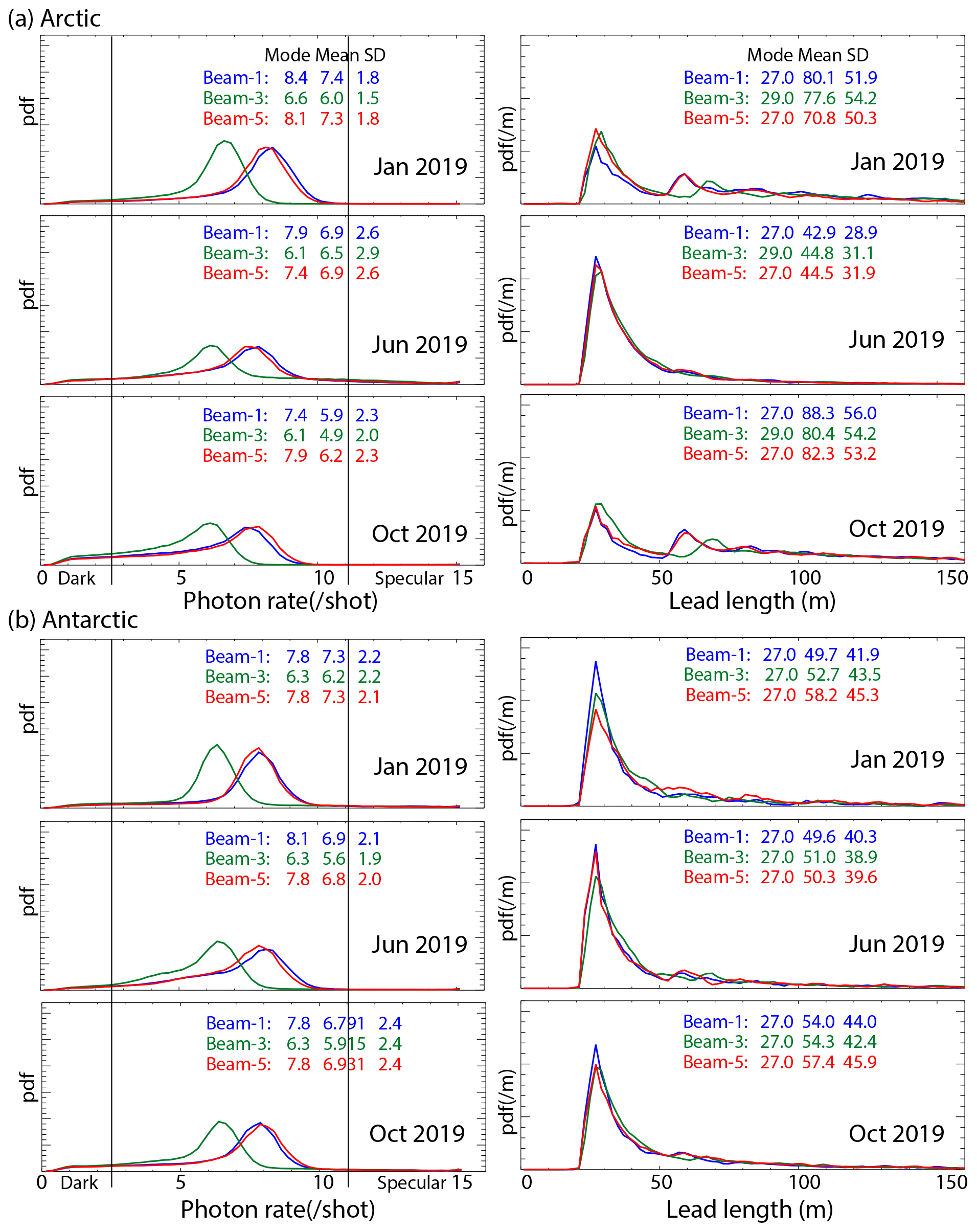
Figure 1 Distributions of photon rates of all height segments and lead lengths (strong beams) in IS-2 sea ice products of the (a) Arctic and (b) Antarctic for the months of January, June and October 2019. Numerical values show the mode, mean and standard deviation of the distributions.

3.3 Photon rates and length of sea surface height segments

Figure 1 shows the distribution photon rates (photon / shot) and lead lengths of the sea surface height samples (strong beams). The mean photon rates of the entire height population (between ∼6–8, Fig. 1 – left panel) are dominated by the expected returns from a mixture of snow-covered sea ice of different roughness. The distributions are remarkably consistent for the 3 months (January, June and October 2019) shown here. As expected, Beam 3 has consistently weaker surface returns. This is due to the lower transmitted laser energy (transmitted energy of Beam 3 is ∼0.81 % of Beam 1 and 5) and thus lower return for this beam, which is consistent with pre-launch expectations and is attributable to the custom construction of the optical component used to split the laser energy into the six IS-2 beams (Neumann et al., 2019). A consequence of this is that it takes more pulses (longer along-track distance) to construct a 150-photon aggregate for surface finding – hence the longer lead lengths seen in Fig. 1.

Because a fixed number of photons are used in surface finding, photon rates are determined by the number of shots, or along-track distance, needed to construct these 150-photon aggregates. That is, the segment length adapts to changes in photon rates from surfaces of different reflectance: height segment lengths are longer when the returns are lower, and vice versa. The distributions of lead lengths (aggregate of sea surface segments described above) – used in reference height calculations – are bi-modal (Fig. 1 – right panel); the modes are determined by leads that are specular or quasi-specular and by leads with very low reflectance. The lead lengths vary between ∼10 and 150 m, with modes at ∼27 m (specular leads) and ∼60 m (dark leads). The upper bound in segment length (∼150–200 m) is controlled by a setting in the surface-finding procedure that restricts the distance over which photons are aggregated and serves to reduce the number of noise and background photons accumulated in long-distance aggregates. The consequences of a longer integrating distance for estimating surface heights of dark leads are (1) the likelihood that there is a mixture of surface types in the height segment and (2) the higher number of accumulated noise photons in the larger number of shots used.

For estimating the reference surface heights, the specular and dark-lead heights (in R001 and R002) are mixed in the weighting process above.

4 Effects of clouds on leads with low surface reflectance

As mentioned above, the presence of clouds reduces the surface returns (i.e., lowers the photon rates) because the transmitted or reflected energy is scattered away from the field of view of the lidar. In this section, we illustrate the effect of clouds on the classification of low-reflectance surfaces. First, we show the phenomenology in two examples from coincident IS-2 and CAMBOT observations acquired in April 2019. Second, we examine the distributions of sea surface heights in the population of specular and dark leads used in reference surface estimation. Third, we assess the fraction of the dark-lead population that is likely contaminated by clouds.

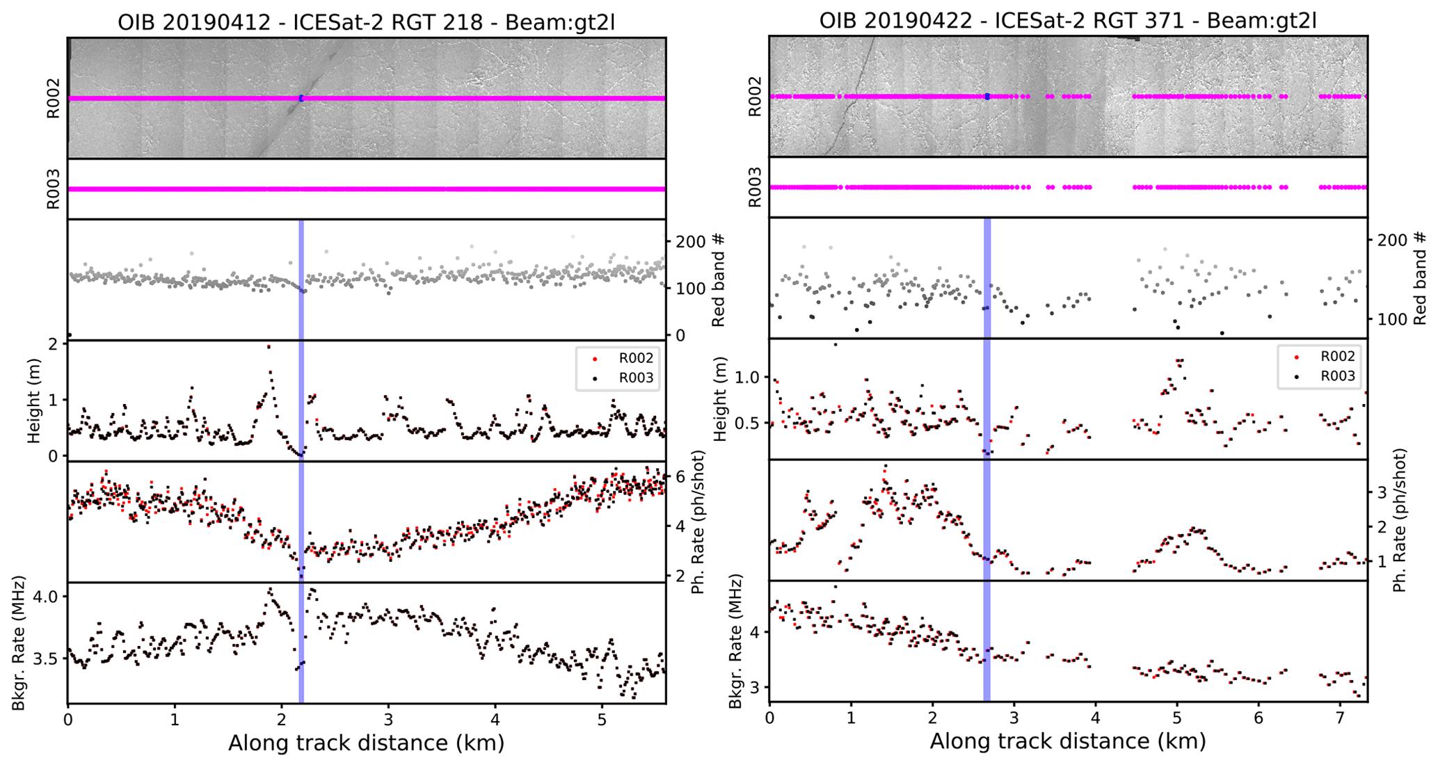
Figure 2 Effect of clouds on IS-2 photon rates, background rates and surface-type classification in IS-2 in R002 and R003 on (left) 12 April 2019 (RGT-218) and (right) 22 April (RGT-371). Top: ATL10 overlaid on CAMBOT RGB imagery, with magenta markers indicating sea ice segments and blue indicating sea surface (smooth dark lead) in R002 ATL10; second panel: magenta markers indicating sea ice segments in R003 (there are no lead segments); third panel: red band intensity in the CAMBOT RGB image at the location of the ATL10 segments; fourth panel: ATL10 surface height; fifth panel: ATL10 photon rate; sixth panel: ATL10 background rate. In panels 4–6, red represents R002 and black represents R003. The vertical blue shading shows the location of the ATL10 sea surface reference (smooth dark lead) segment in R002. Low contrast in the CAMBOT imagery is due to low solar elevations of 8 and 11^∘ during acquisition.

4.1 Phenomenology

In the presence of clouds, the photon rates are unreliable proxies of brightness or apparent surface reflectance of the surface. In the first CAMBOT–IS-2 scene (Fig. 2a), the attenuation effects of atmospheric moisture are evident in the coincident coverage of a “dark” lead detected by the surface-type classifier (Fig. 2a). A clear indication of the presence of clouds is the concurrent along-track decreases in IS-2 photon rate (from ∼6 to ∼2 photons / shot) and increases in background rate (from ∼3 to 4 MHz), followed by a recovery of both parameters to close to their expected levels. Since a dip in the recorded levels of the CAMBOT data is not seen, the clouds are likely present in the atmospheric column above the altitude of the IceBridge platform, which was ∼1000 m for this flight line. Because of the attenuated photon rates, the IS-2 samples within the linear feature (refrozen lead) in the CAMBOT image were mislabeled as a dark lead by the surface classifier. In the absence of the attenuation effects (dip in photon rates), these samples would not have been classified as a dark lead. Even though the post-classification height filter ensured that the surface height of those samples was the lowest in the neighborhood, the sampled heights are unlikely indicative of the sea surface (i.e., they are higher than the actual sea surface).

The second example shows gaps in IS-2 surface retrievals near the center of the CAMBOT image. Gaps in IS-2 data are present when the software on board the IS-2 observatory determines, by an onboard analysis of the photon density in that atmospheric column, that surface returns are unlikely to be present; thus no data are telemetered or downlinked to the ground station. This suggests the presence of clouds in the neighborhood of the gaps. In fact, large variability in photon rates and CAMBOT data is seen away from the gaps. Since this type of surface variability is unlikely from the sea ice cover in an area north of Ellesmere Island on 22 April, both the IS-2 and CAMBOT data are affected by the atmosphere. Again, there is a misclassified lead near the center of the image – with a distinct dip in the surface height – even though a correct surface classification would have removed those samples as candidate sea surface segments. These two examples highlight the potential effects of clouds in surface-type classification.

Why are cloud flags not used? The crucial element in freeboard retrieval is the accurate identification of the height samples that are suitable for estimation of the local sea surface, largely because of the low density of these samples on the ice cover, and errors in reference heights affect freeboard estimates over 10 km length scales, unlike the impact of errors in individual ice surface height estimates. The cloud flags in IS-2 are sampled every 400 m and not compatible with the size of the leads used here (27–80 m). Also, we find that the cloud flags are quite conservative: our understanding to date is that a large number of leads would be removed if the cloud flags were used to filter the returns. The IS-2 cloud flags, as they are currently designed, are thus currently ineffective for addressing the cloud issue at the length scale of the leads in the sea ice data.

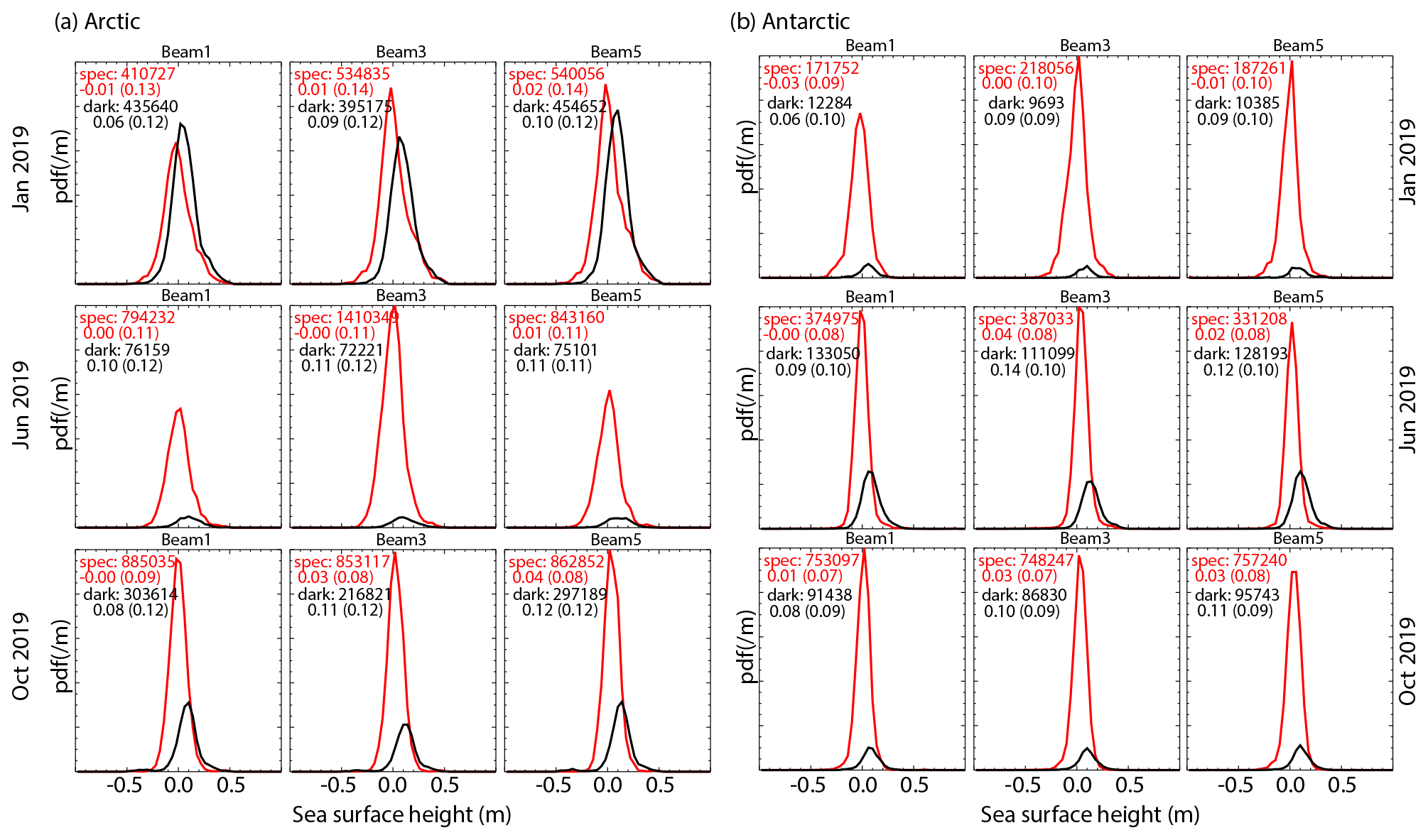
Figure 3 Distribution of surface heights classified with specular (red) and dark returns (black) in the (a) Arctic and (b) Antarctic IS-2 sea ice products for the months of January, June and October 2019. All height segments are subject to additional height filtering in the determination of reference surfaces used in freeboard calculations. Numerical values show the mean and standard deviation of the distributions.

4.2 Sea surface height distribution of specular and/or dark leads

In first and second releases of the IS-2 sea ice products (R001 and R002), both specular and dark leads were used in the determination of the local (10 km) sea surface references. Here, we examine the height distributions of the population of specular and dark leads used in reference surface estimation to assess whether the distributions of dark leads introduce biases in the freeboard calculation. The height distributions of the two surface-type categories in the Arctic and Antarctic for 3 months in 2019 (January, June and October) are shown in Fig. 3. We summarize the results as follows:

• The height distributions overlap even though the mean of the height distribution of dark leads is higher by up to 10 cm: the modes of the distributions are skewed relative to each other, and the differences in the negative tail of the distribution are more distinct. This provides further, albeit indirect, evidence that the height distribution of the dark leads is contaminated by incorrect classification of the surface as discussed above.

• The population of height segments classified as specular is much higher than the population classified as dark leads, except for the January 2019 Arctic distributions, meaning the overall impact and significance of the dark leads are lower.

It should also be noted that these are distributions of the sea surface height segments prior to their aggregation into leads and the weighted averaging of these segments into 10 km reference height estimates for freeboard calculations. Thus, the impact of the dark leads is further moderated in cases where there is a mixture of specular and dark-lead segments in a given 10 km section. The impact on monthly composites of the Arctic and Antarctic is discussed in Sect. 5.

4.3 Towards a new contrast ratio cloud or lead filter

We have examined a simple approach to identifying the fraction of dark leads that may be affected by clouds (for possible implementation in future data releases but not R003). In the approach, the photon rate of a dark lead (PR_lead) is compared to the height segment with the highest photon rate (PR_max) in the neighborhood of the dark lead. As a simple diagnostic, we calculate the contrast ratio:

$$R={\displaystyle \frac{{\text{PR}}_{\max }}{{\text{PR}}_{\mathrm{lead}}}}.$$

Under cloud-free and ideal conditions, we expect the contrast to be between 8 and 9; i.e., the albedo of snow-covered sea ice is >0.8 compared to the lower albedo (reflectance) of smooth open leads of ∼0.1. In less-than-ideal conditions (e.g., cloudy conditions), however, we expect this contrast to be lower.

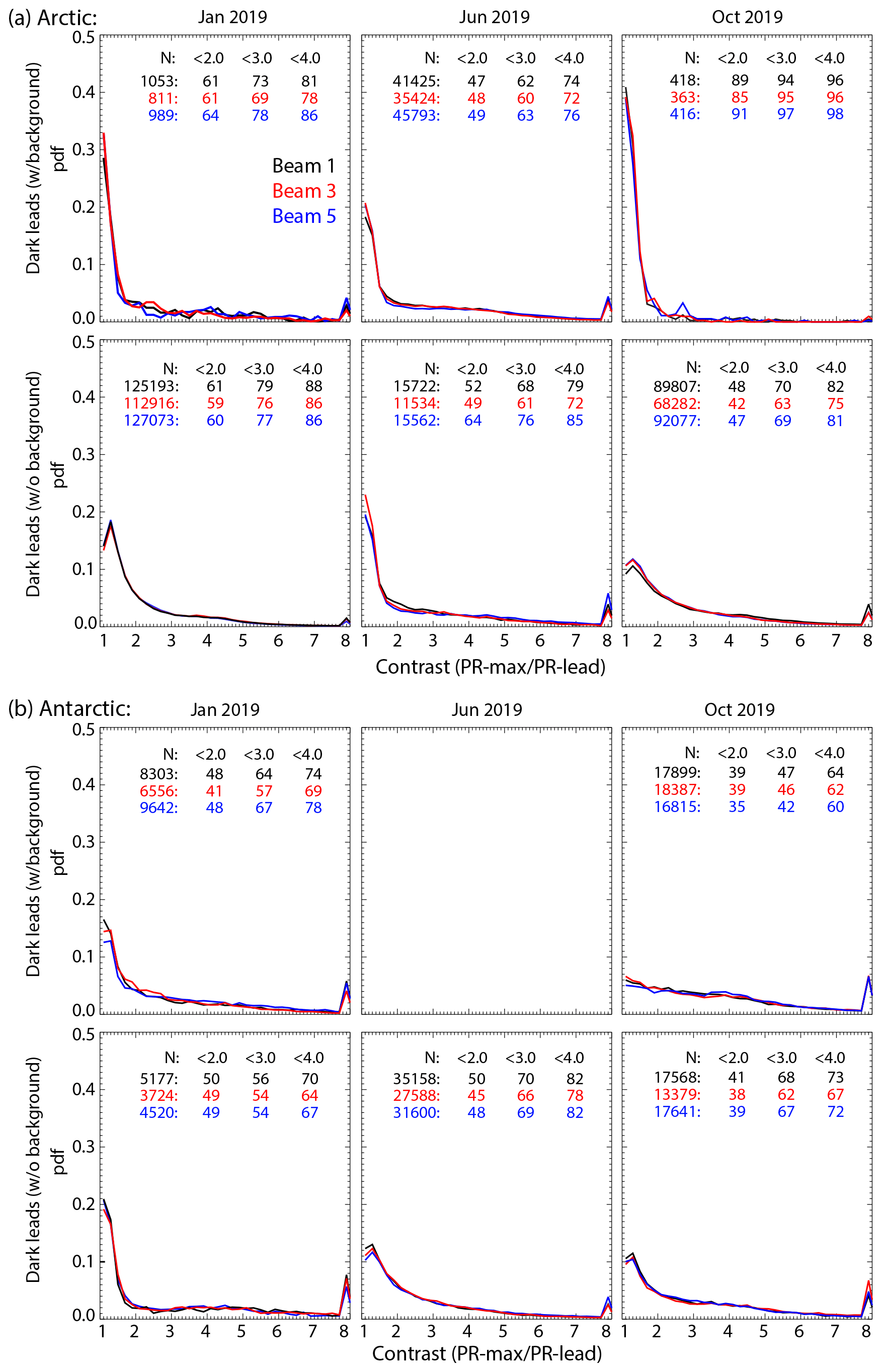
Figure 4 Contrast of lead photon rate (PR-lead) with surface segment with the highest photon rate (PR-max) within ±20 km of the “dark” lead for the months of January, June and October 2019. Numerical values show the number of surface height segments classified as dark lead and the percentage of the population with contrast (PR-leads $/$ PR-max) <2.0, <3.0 and <4.0.

Figure 4 shows the percentage of the dark-lead population with contrasts <2, <3 and <4 within a ±20 km neighborhood of the dark lead. It is evident that 70–80 % of the population (for the months shown here) have a contrast ratio <4 and are potentially misclassified if clouds were not considered in the surface-type analysis. This preliminary analysis suggests that this local contrast ratio diagnostic could provide a useful filter to address the cloud misclassification issue. However, the effectiveness and the implementation of this approach need to be examined in more detail if this is to be incorporated into the next IS-2 sea ice product generation.

5 An algorithm revision: R001 and R002 to R003

In this section, we describe a simple revision to our current product generation algorithm – implemented for R003 – to eliminate the potential effects of the misclassified dark leads. Next, we show the differences between R001 and R002 on the one hand and R003 on the other in the monthly freeboard distributions and composites of the Arctic and Antarctic sea ice covers for January, June and October 2019.

5.1 Algorithm revision

In R001 and R002, candidate height segments that were selected to estimate reference heights for freeboard calculations included, as discussed above, two primary surface types: specular and smooth dark leads. Given the likelihood of the mislabeling of dark-lead segments as suggested by the results presented here, a simple revision to the algorithm for production of R003 has been implemented. Instead of using two surface types for reference height calculation, only the specular surface returns are used to derive the reference sea surface. This is a simple change in the software system, chosen to enable continued sea ice product generation while a more sophisticated filtering approach (as highlighted in the previous section) is tested. The overall impact of this change in the freeboard estimates is shown in the next section.

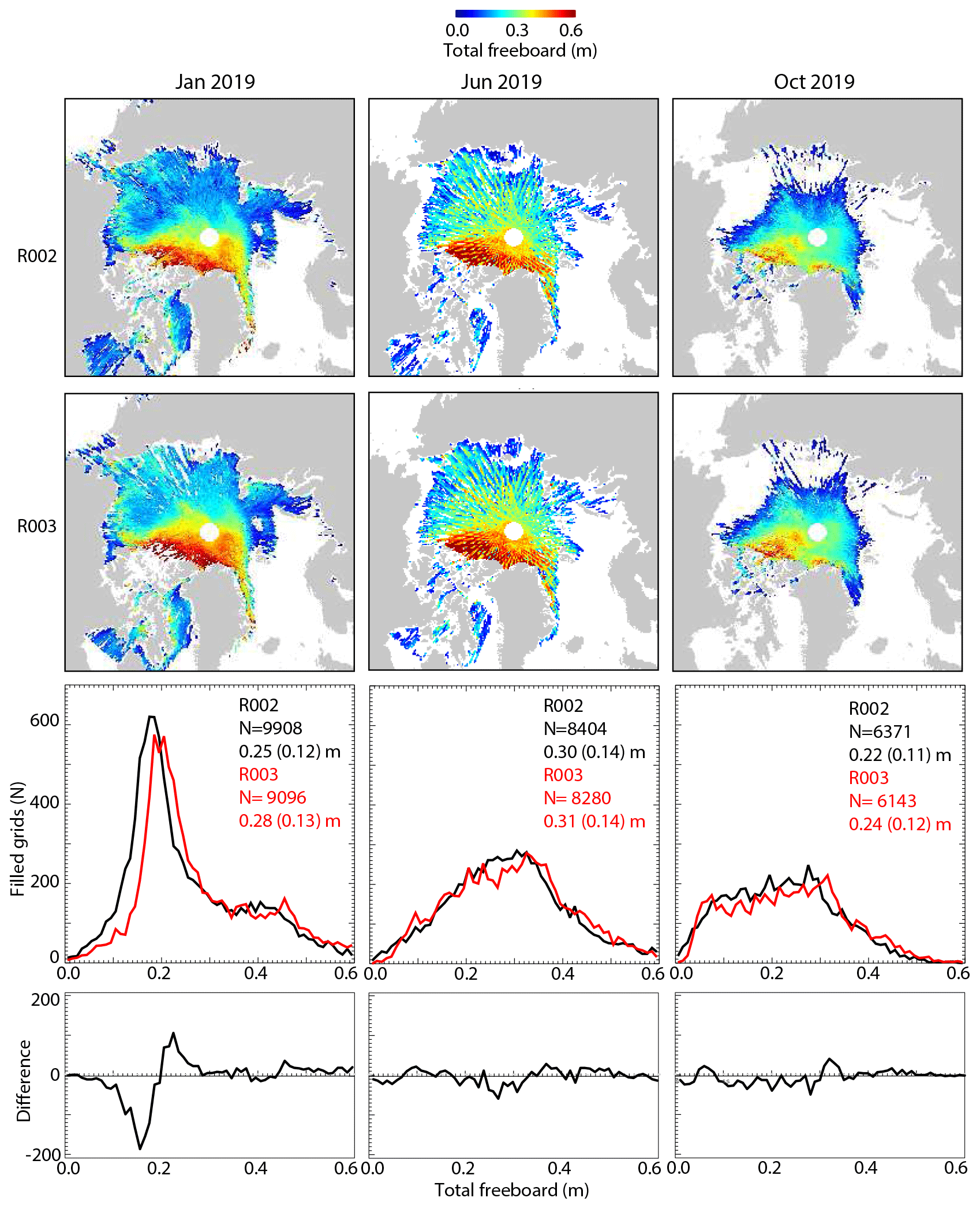
Figure 5 Differences of monthly composite freeboard statistics and coverage between Releases 002 and 003 in the Arctic IS-2 sea ice products for the months of January, June and October 2019. Only specular leads are used in Release 003. N is the number of grid cells (25 by 25 km) that are covered, and numerical values show the mean and standard deviation of the composite field.

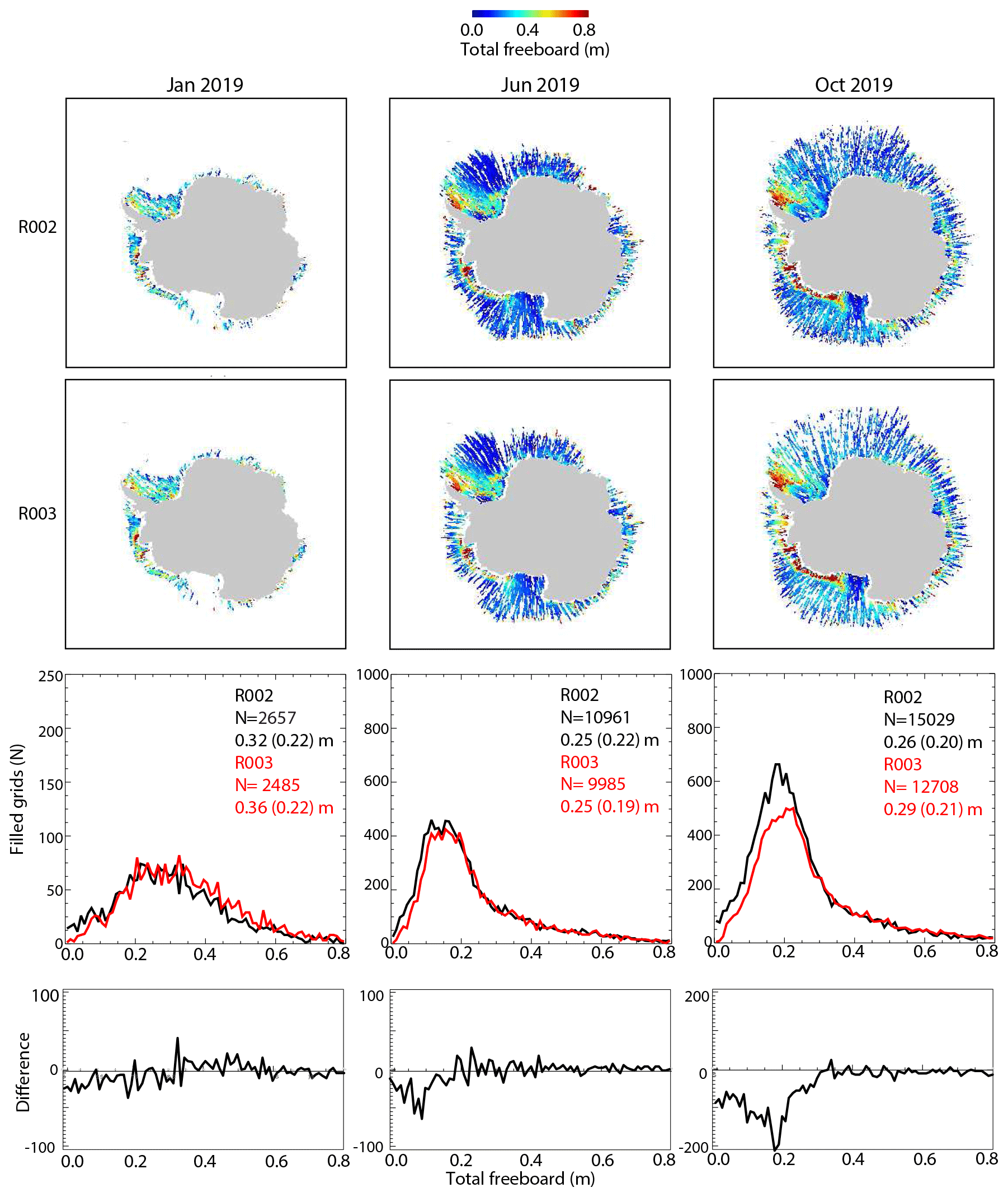
Figure 6 As in Fig. 5 but for the Antarctic.

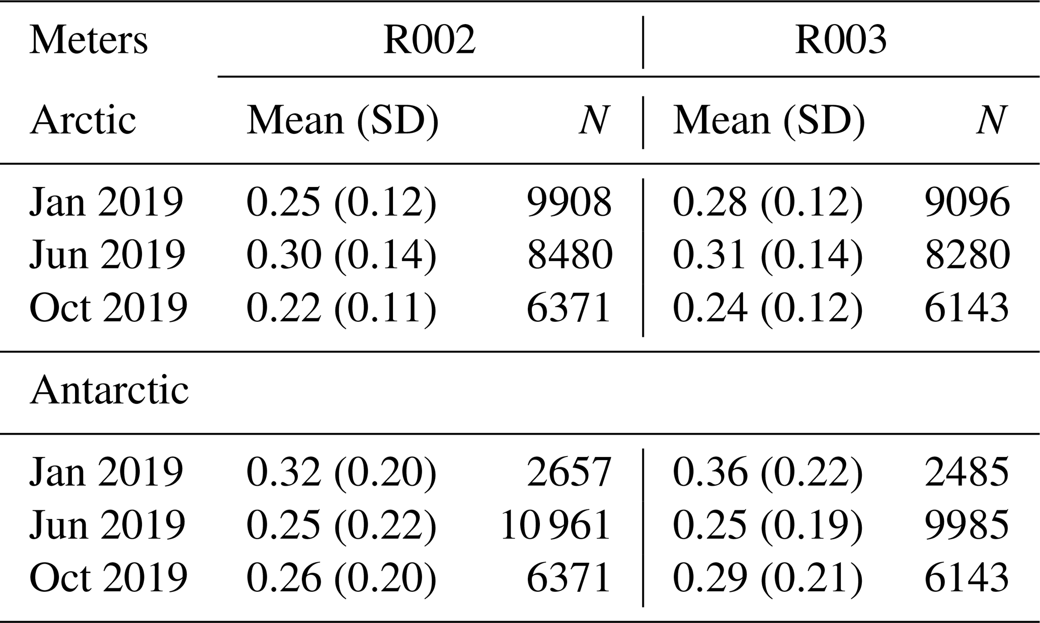
Table 1 Comparison of summary statistics and grid coverage of freeboard retrievals for the 3 months over the Arctic and Antarctic sea ice cover shown in Figs. 5 and 6. N is the number of grid cells (25 km) with freeboard retrievals.

5.2 Differences between R002 and R003

Here, we compare the retrievals from R002 and R003 for the months of January, June and October 2019. The consequence of this change can be seen in the freeboard composites and distributions of the Arctic and Antarctic sea ice covers (Figs. 5 and 6), and Table 1 summarizes the freeboard statistics of the distributions. The differences are summarized below:

• In the monthly composites of the Arctic and Antarctic, area coverage has decreased by ∼10–20 % because, due to excluding the dark leads, there are fewer estimates of the local reference sea surface for freeboard calculations.

• The composite means have increased by 0–4 cm because of the use of surface heights from only specular returns in freeboard calculations. As shown in the previous section, the use of specular returns would lower the sea surface estimates and thus increase the retrieved freeboard. We also note that some of the changes are due to changes in coverage as well. The overall impact of dark leads on freeboard statistics is also dependent on the relative population of specular and dark leads. In January 2019, the two populations are comparable (Fig. 3), whereas the dark-lead populations are smaller in the other months in the Arctic and Antarctic.

In repeating a comparison of near-coincident freeboards from IS-2 and IceBridge in Kwok et al. (2019b), the four available sea surface references in the earlier release were not retrieved by the revised algorithm (R003). This gives an indication that the sea surfaces used in that analysis were dark leads (i.e., not classified as sea surfaces in R003) and no longer designated as sea level references (in R003) for use in ATL10 freeboard calculations. This also suggests that the lower IS-2 freeboards (compared to those from IceBridge) in that analysis may be due to the impact of dark leads, i.e., higher (biased) sea surfaces and thus lower IS-2 freeboard estimates, consistent with our expectation.

The increased freeboards correspond to an increase in ice thickness and snow depth estimates from ICESat-2 first examined in Petty et al. (2020) and Kwok et al. (2020b). These are not addressed in this paper because the present focus is on the publicly available ICESat-2 sea ice freeboard product distributed by the ICESat-2 mission. The impact on sea ice thickness and snow depth will be addressed in forthcoming papers.

6 Conclusions

In this paper, we examine the effect of clouds on the surface-type classifier used to identify sea surface samples for determining freeboard. Based on these results, the IS-2 sea ice classification has been revised for production of Release 003 of the IS-2 ATL07 (sea ice heights) and ATL10 (freeboard) products.

In R001 and R002, candidate height segments that were selected to estimate reference heights for freeboard calculations included two surface types: specular and smooth dark leads. We found that the photon rates, used as proxies of surface reflectance, are attenuated due to clouds (leading to incorrect classification of dark leads), and surface heights from dark leads are sometimes biased relative to the heights from the more reliable specular returns. This results in reference surfaces that are higher (when weighted with heights of specular leads), thus lowering the estimated freeboards. Cloud flags from ATL09 are low resolution (∼400 m) and thus do not provide an effective filter at the length scales of leads (tens of meters) detected by ICESat-2.

In R003, we revised the surface reference calculations so that only leads with specular returns are used. The consequence of the changes can be seen in the freeboard distribution composites of the Arctic Ocean and of the Antarctic. Broadly, for the 3 months examined here, coverages have decreased by ∼10–20 % because there are fewer leads (due to excluding the dark leads), and the composite freeboard means have increased by 0–4 cm because of the use of surface heights from more reliable specular surfaces (i.e., closer to the local sea surface) in freeboard calculations.