the Creative Commons Attribution 4.0 License.
the Creative Commons Attribution 4.0 License.
 | 09 Feb 2021
Distributed summer air temperatures across mountain glaciers in the south-east Tibetan Plateau: temperature sensitivity and comparison with existing glacier datasets
Wei Yang
Álvaro Ayala
Claudio Bravo
Chuanxi Zhao
Francesca Pellicciotti
Near-surface air temperature (Ta) is highly important for modelling glacier ablation, though its spatio-temporal variability over melting glaciers still remains largely unknown. We present a new dataset of distributed Ta for three glaciers of different size in the south-east Tibetan Plateau during two monsoon-dominated summer seasons. We compare on-glacier Ta to ambient Ta extrapolated from several local off-glacier stations. We parameterise the along-flowline sensitivity of Ta on these glaciers to changes in off-glacier temperatures (referred to as “temperature sensitivity”) and present the results in the context of available distributed on-glacier datasets around the world. Temperature sensitivity decreases rapidly up to 2000–3000 m along the down-glacier flowline distance. Beyond this distance, both the Ta on the Tibetan glaciers and global glacier datasets show little additional cooling relative to the off-glacier temperature. In general, Ta on small glaciers (with flowline distances <1000 m) is highly sensitive to temperature changes outside the glacier boundary layer. The climatology of a given region can influence the general magnitude of this temperature sensitivity, though no strong relationships are found between along-flowline temperature sensitivity and mean summer temperatures or precipitation. The terminus of some glaciers is affected by other warm-air processes that increase temperature sensitivity (such as divergent boundary layer flow, warm up-valley winds or debris/valley heating effects) which are evident only beyond ∼70 % of the total glacier flowline distance. Our results therefore suggest a strong role of local effects in modulating temperature sensitivity close to the glacier terminus, although further work is still required to explain the variability of these effects for different glaciers.
- Article
(7068 KB) - Full-text XML
- Companion paper
-
Supplement
(575 KB) - BibTeX
- EndNote


Near-surface air temperature (Ta) is one of the dominant controls on glacier energy and mass balance during the ablation season (Petersen et al., 2013; Gabbi et al., 2014; Sauter and Galos, 2016; Maurer et al., 2019; Wang et al., 2019), though modelling its spatio-temporal behaviour above melting ice surfaces remains a challenge. The absence of distributed information regarding Ta has favoured the use of simple, space–time invariant relationships of Ta with elevation, typically that of the free-air environmental lapse rate (ELR). A free-air ELR cannot be reliably used to estimate near-surface air temperatures above melting glaciers, where steep gradients are found within 10 m of the surface under warm ambient (off-glacier) conditions (van den Broeke, 1997; Greuell and Böhm, 1998; Oerlemans, 2001; Oerlemans and Grisogono, 2002; Ayala et al., 2015). As a result, any extrapolation of Ta observations from an off-glacier location, particularly those at lower elevations, are likely to lead to an overestimation of snow and ice ablation in energy balance and enhanced temperature index melt simulations (e.g. Petersen and Pellicciotti, 2011; Pellicciotti et al., 2014; Shaw et al., 2017). While models applying the degree day approach can make use of off-glacier temperatures as forcing because they are heavily reliant on calibration, for energy balance models and models of intermediate complexity (Pellicciotti et al., 2005; Ragettli et al., 2016) it is key to resolve the air temperature distribution over glaciers, especially for turbulent flux calculations and typical parameterisations of incoming longwave radiation.
This problem has been long understood (Greuell et al., 1997; Greuell and Böhm, 1998), but only within the last decade have studies approached it in more detail (Petersen et al., 2013; Ayala et al., 2015; Carturan et al., 2015; Shaw et al., 2017; Bravo et al., 2019a; Troxler et al., 2020). Until recently, modelling studies have relied upon simple lapse rates (including the ELR) and/or single bias offset values to account for the cooling effect of the near-surface air on glacier (Arnold et al., 2006; Nolin et al., 2010; Ragettli et al., 2016). The variations of Ta along the glacier flowline (defined following Shea and Moore, 2010, as the horizontal distance from an upslope summit or ridge), however, are much more complex (Ayala et al., 2015; Shaw et al., 2017), though a lack of available data usually restricts one's ability to appropriately model this variable.
To date, two main, simplified model approaches have been developed and tested to represent air temperature over glaciers (Fig. 1a). The first is the statistical model by Shea and Moore (2010) developed to reconstruct Ta across glaciers of varying size in western Canada from ambient temperature records. This approach considered the ratios of observed on-glacier temperature and estimated ambient temperature for the elevation of a given point on a glacier (hereafter TaAmb). The authors calculated two ratios from a piecewise regression above and below a critical threshold temperature for the onset of the glacier katabatic boundary layer (KBL – see Sect. 4.3). The parameterisations that operate as a function of the along-flowline distance have since been tested by Carturan et al. (2015) and Shaw et al. (2017) on smaller glaciers in different parts of the Italian Alps. Carturan et al. (2015) found that the original published parameterisations were sufficient to explain Ta on small, fragmenting glaciers up to flowline distances of ∼2000 m. However, investigation by Shaw et al. (2017) on a small alpine glacier found a pattern of along-flowline Ta that was better described by an alternative, thermodynamic model approach. This second, physically oriented approach was developed by Ayala et al. (2015) to account for a relative warming effect evident on the termini of some mountain glaciers when compared to upper elevations. The modified model (termed “ModGB” in the literature) accounts for the down-glacier cooling of Ta at increasing flowline distances due to sensible heat exchange and adiabatic heating (Greuell and Böhm, 1998). It adds a warming factor based upon on-glacier observations in the lower sections of the glacier (e.g. at the greatest flowline distances) to account for additional processes of adiabatic warming (Ayala et al., 2015) (Fig. 1a). The ModGB approach has been successively applied at other glacier sites around the world (Shaw et al., 2017; Troxler et al., 2020), though the question of its transferability remains open (Troxler et al., 2020).
In this way, the ModGB method operates on the physical principles of the glacier boundary layer (Greuell and Böhm, 1998), though it corrects for relative warming on the lower portion of glacier (Ayala et al., 2015). To establish the magnitude of this warming, however, along-flowline data in the lower portion of the glacier are essential. Because the available distribution of on-glacier observations is often limited and rarely extends for the entire length of the glacier flowline, this additional correction for warming associated with the unknown parameters of ModGB can lead to high variability in Ta estimates on the lower glacier ablation zone (Troxler et al., 2020) (Fig. 1a). In contrast to this, the statistical method of Shea and Moore (2010) provides a more simplified estimation that has fewer assumptions and parameters, though it does not explicitly account for physical processes thought to be the cause of relative warming on the glacier terminus. It also provides a parameter that more explicitly represents the glacier temperature sensitivity of the on-glacier Ta (defined here as the ratio of changes in observed Ta on glacier to changes in TaAmb – Fig. 1b and c). Despite its more conceptual nature, because of its ease of applicability, typical of a more simplistic statistical approach, we adopt the Shea and Moore (2010) method to further investigate along-flowline Ta in this study.
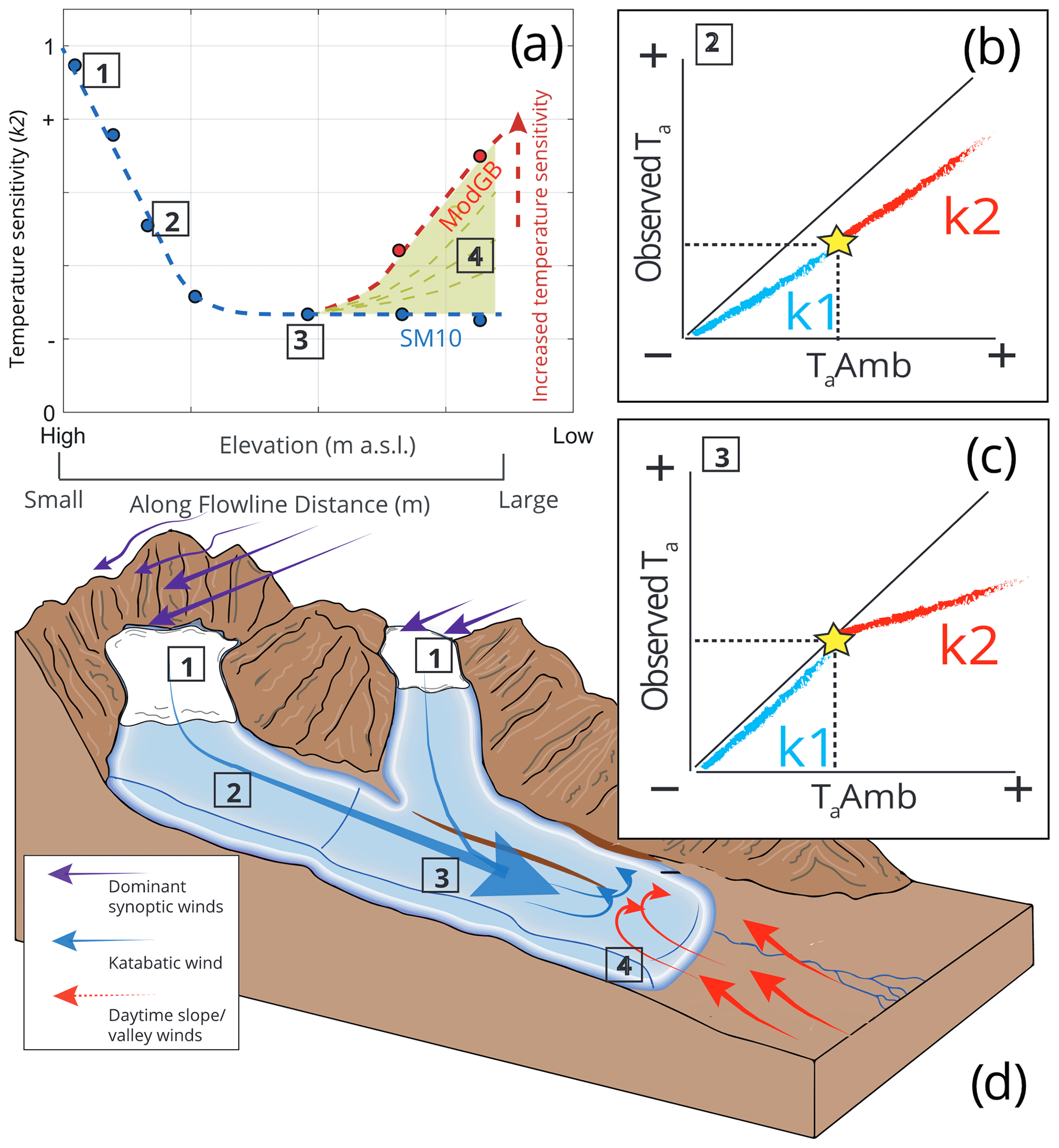
Figure 1A schematic diagram to describe the temperature sensitivity of on-glacier air temperature (Ta) to the extrapolated ambient temperature (TaAmb) at given elevations/flowline distances on a mountain glacier. Points 1–4 indicate locations of interest that are linked between panels. Panel (a) indicates the along-flowline k2 temperature sensitivities to TaAmb, considering the differences represented by the models of SM10 and ModGB for glacier termini (see text). Panels (b) and (c) represent the differences of k1 (blue) and k2 (red) sensitivities observed in the data at different theoretical locations on the glacier, the latter of which shows the theoretical parameterisation presented by Shea and Moore (2010). The yellow stars indicate the calculated threshold for katabatic onset (T* in the text). Panel (d) represents an idealised case of katabatic and valley/synoptic wind interactions that potentially dictate the along-flowline structure of on-glacier temperature sensitivity and thus Ta estimation.
To date, few studies have investigated the variability of distributed, on-glacier Ta at different sites around the world. As such, the transferability of temperature estimation models and/or model parameters remains mostly unknown, and analysis of individual glacier sites, while beneficial to process understanding, may not advance the science on how to treat the on-glacier Ta in models. In this study, we use new datasets of on-glacier temperature observations on three glaciers of varying size in the south-east Tibetan Plateau. We analyse the main controls on along-flowline Ta and its temperature sensitivity and present these new findings in the context of 11 other on-glacier observations around the world.
Specifically we aim to (i) understand the variability of Ta with the along-flowline distances at three glaciers in the south-east Tibetan Plateau, (ii) identify and quantify the temperature sensitivity of on-glacier Ta for different meteorological conditions and glacier sizes, and (iii) parameterise the along-flowline Ta using the Shea and Moore (2010) method for the Tibetan glaciers and discuss it in the context of globally derived, published datasets of on-glacier air temperatures.
The study glaciers are located in the upper Parlung Zangbo (also know as the Parlung Tsangpo) river catchment in the south-east Tibetan Plateau (29.24∘ N, 96.93∘ E – Fig. 2), a region characterised by a summer monsoon climate that typically intrudes via the Brahmaputra Valley (Yang et al., 2011). We present data for three maritime-type valley glaciers in the Parlung Zangbo catchment: Parlung Glacier Number 4 (hereafter Parlung4), Parlung Glacier Number 94 (Parlung94) and Parlung Glacier Number 390 (Parlung390). Parlung4 (Fig. 2d) is ∼10.8 km2, is north-north-east facing and has an elevation range of 4659–5939 (Ding et al., 2017). Glaciers Parlung94 (Fig. 2c) and Parlung390 (Fig. 2e) are smaller valley glaciers (2.51 and 0.37 km2, respectively) that have termini at higher elevations (elevation ranges of 5000–5635 and 5195–5469 , respectively). The glaciers of the catchment were classified by Yang et al. (2013) as having a spring-accumulation regime and the longest rain season of the entire Tibetan Plateau. The upper Parlung Zangbo river catchment has a mean summer (1979–2019) annual air temperature of ∼2 ∘C (at 4600 ), and temperatures in the wider region have been shown to be increasing since the mid-1990s (Yang et al., 2013). The glaciers of this region have been shown to be very sensitive to temperature changes, though with a lower sensitivity of mass balance to elevation compared to other continental glaciers of the Tibetan Plateau (Wang et al., 2019). Because Tibetan glaciers are shrinking and fragmenting, the accurate estimation of on-glacier temperatures is relevant for investigating and modelling their temperature sensitivity (Carturan et al., 2015). However, to date, no studies regarding the distribution of on-glacier temperature have been performed within the Tibetan Plateau.
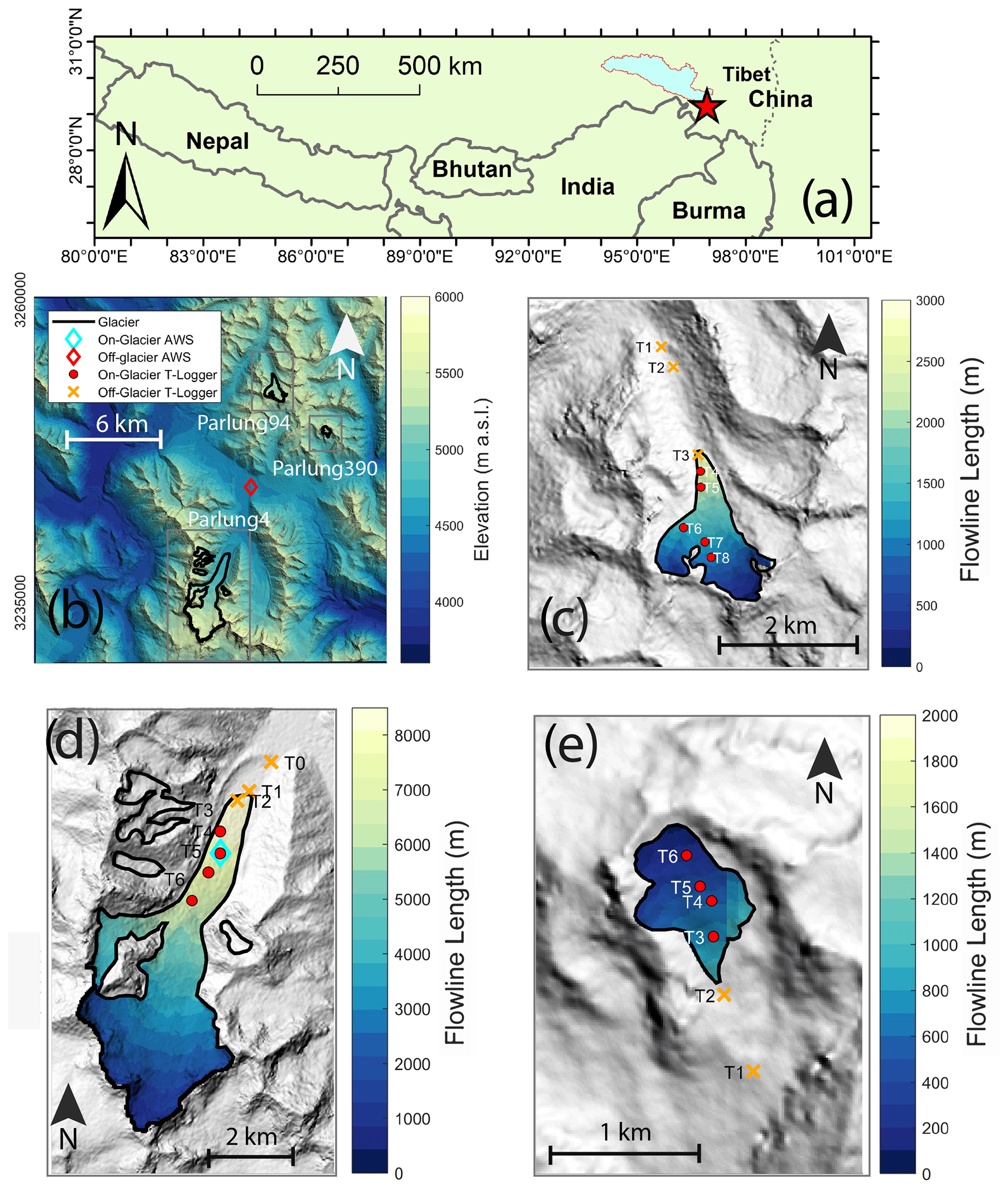
Figure 2The location of Parlung catchment in Tibet (a) and a map of the Parlung glaciers (b) with the study glaciers, Parlung94 (c), Parlung4 (d) and Parlung390 (e). Off-glacier and on-glacier AWS and T-logger locations are shown (without glacier number suffix – see Table 1). Panel (b) shows the elevation of the catchment (DEM source: Alos Palsar), and Panels (c)–(e) show the calculated flowline distances based upon TopoToolbox (scales vary).
3.1 Meteorological observations
We present the observations of Ta from a total of 20 air temperature logger locations (Table 1), 13 of which are situated on glacier (4680–5369 ) and seven off glacier (4648–5168 ). These stations (hereafter referred to as “T loggers”) observed Ta at a 2 m height using HOBO U23-001 temperature–relative-humidity sensors (accuracy +0.21 ∘C) within double-louvred, naturally ventilated radiation shields (HOBO RS1) mounted on free-standing tripods. The T loggers recorded data in 10 min intervals that are averaged to hourly data for analysis. We identify a common observation period over the summers of 2018 and 2019 that ranges from 12 July–18 September. For these date ranges, we observe only small data gaps for some T loggers (<1 % of the total period). We apply the nomenclature of TXG, whereby X refers to the T-logger number on each glacier and G refers to the glacier number (Table 1).
Table 1Details of each AWS/T-logger station used in this analysis including the calculated flowline distances.
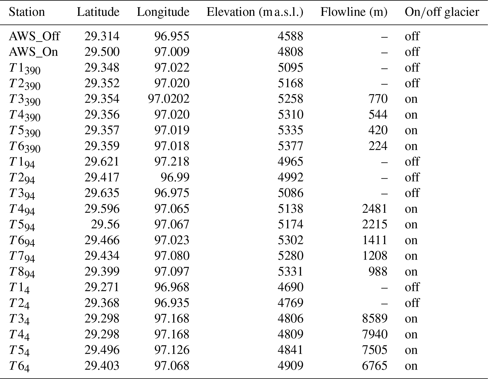
We additionally present Ta observations at two automatic weather stations (AWS) at elevations ∼4600 (off glacier, henceforth AWS_Off) and ∼4800 (on Parlung4, henceforth AWS_On) for the same time period (Fig. 2). The AWS Ta observations are provided by Vaisala HMP60 temperature–relative-humidity sensors (accuracy +0.5 ∘C) housed in naturally ventilated, Campbell 41005-5 radiation shields. We obtain information regarding incoming shortwave radiation and relative humidity (AWS_Off), on-glacier wind speed (AWS_On), and free-air wind speed and direction (ERA5 – C3S, 2017). We use these data to explore the relationships of hourly on- and off-glacier temperatures (Sect. 4.2) for different prevailing conditions.
3.2 Intercomparison of air temperature observations
To evaluate the comparability of air temperature measurements, we calculate the hourly divergence of two naturally ventilated Ta observations for the whole period between T44 and AWS_On (Fig. 2d), which are located within a few metres of horizontal distance of each other on Parlung4 Glacier. A test of absolute differences between the two stations resulted in a mean of <0.4 ∘C for all hours (n=3312) and ∼0.5 ∘C for the warmest 10 % of the hours of ambient temperature at AWS_Off. We find that for these warm hours (hereafter referred to as “P90” – Ayala et al., 2015; Shaw et al., 2017; Troxler et al., 2020), when the KBL development is theoretically at its strongest (e.g. van den Broeke, 1997; Oerlemans and Grisogono, 2002), 95 % of hourly differences were <1 ∘C (Fig. S1 in the Supplement). For on-glacier stations at large flowline distances (Fig. 2), large differences are considered less likely given the good ventilation provided to the sensors within the KBL. While observations at short flowline distances with calm conditions and high incoming radiation may result in larger differences up to ∼1 ∘C (Troxler et al., 2020), we apply a ±0.5 ∘C uncertainty for analysis of distributed Ta. For the instantaneous differences >1 ∘C, wind speeds at AWS_On were <2 m s−1. Wind speeds for P90 conditions were otherwise in excess of 3–4 m s−1, though no other observations of on-glacier wind speed are available at higher elevations. We note that in the absence of an artificially ventilated Ta measurement as a reference (e.g. Georges and Kaser, 2002; Carturan et al., 2015), a true uncertainty value cannot be prescribed for the Ta observations of our study and only assumed based upon previous literature. This is discussed further in Sect. 6.
3.3 Elevation information
We use the 12.5 m Alos Palsar (ASF DAAC, 2020) digital elevation model (DEM) to obtain elevation information for the catchment (Fig. 2b). Flowline distances (m) for each glacier are calculated from the TopoToolbox functions in MATLAB (Schwanghart and Kuhn, 2010), following Troxler et al. (2020). We note that the methodology for flowline generation is not currently uniform among all studies of this type (Shea and Moore, 2010; Ayala et al., 2015; Carturan et al., 2015; Shaw et al., 2017; Bravo et al., 2019a; Troxler et al., 2020) and may produce some differences in the calculated distances close to the lateral borders of the glaciers. In addition, the generated flowlines may also be dependent upon the quality and resolution of the DEM available. However, we do not analyse lateral Ta variations in this study and consider the impact of varying methods for flowline generation to be negligible when assessing observations at a few selected points on the glacier.
Our methods consist of (1) aggregating temperature observations based on off-glacier temperatures and prevailing meteorological conditions, (2) generating off-glacier temperature lapse rates to compare on- and off-glacier temperatures at the same elevation, and (3) estimating the near-surface temperature sensitivity by fitting parameters to the model of Shea and Moore (2010). The following subsections outline the subgrouping (Sect. 4.1) and off-glacier Ta distribution (Sect. 4.2) methodologies. The model parameterisations of Shea and Moore (2010) and application to Tibetan and global datasets are described in Sect. 4.3 and 4.4, respectively.
4.1 Subgrouping on-glacier air temperature observations
Subgrouping allows one to interpret general causal factors that dictate on-glacier behaviour. We subgroup our on-glacier observations by 10th and 90th percentiles (P10 = the coldest 10 %, P90 = the warmest 10 %) of off-glacier Ta at AWS_Off (Fig. 2a). Following the methodology of previous studies (Ayala et al., 2015; Shaw et al., 2017; Troxler et al., 2020), we bin all contemporaneous observations of on-glacier Ta at each T logger that correspond to the same hours as the coldest (P10) and warmest (P90) observations at AWS_Off. We evaluate how strong the linear relationship of on-glacier Ta with elevation and flowline distance is for these subgroups using the coefficient of determination (R2). For a comparison to previous studies (Petersen and Pellicciotti, 2011; Shaw et al., 2017), we also report the equivalent on-glacier lapse rate that would be calculated for the above conditions.
4.2 Comparison of on- and off-glacier air temperature
We extrapolate AWS_Off Ta records to the elevation of each on-glacier T logger (Table 1) to quantify the differences between ambient and on-glacier Ta (Fig. 1a). We derive an hourly variable lapse rate between AWS_Off and off-glacier T loggers T194, T294 and T1390 to construct a catchment lapse rate where the origin of the calculated regression must pass through the elevation of AWS_Off (see Supplement, Fig. S2). These T loggers are assumed to be unaffected by the glacier boundary layer, and we consider this the best available approach to estimate the ambient lapse rate for the catchment. We compare the hourly estimates of the extrapolated off-glacier Ta (TaAmb) with the observations at each on-glacier T logger in order to (i) quantify the differences and how they relate to meteorological conditions and glacier flowline distance and (ii) parameterise the along-flowline temperature sensitivity to TaAmb following Shea and Moore (2010) (Sect. 4.3).
4.3 Estimation of on-glacier temperature sensitivity
The Shea and Moore (2010) approach (hereafter “SM10”) estimates on-glacier Ta using TaAmb at a given elevation by
where T* (∘C) represents the threshold ambient temperature for the onset of katabatic flow and T1 is the corresponding threshold Ta on the glacier. Parameters k1 and k2 are the temperature sensitivities (ratio of on-glacier Ta to TaAmb) below and above the threshold T* (Fig. 1b and c). k1 and k2 were parameterised in the original study using exponential functions of the along-flowline distance (DF):
where βi represents the fitted coefficients. Following the suggestion of Carturan et al. (2015), we implement a relation against the flowline that estimates the threshold temperature for onset of katabatic effects (T*) at a given distance as
where C1 (6.61) and C2 (436.04) are the fitted coefficients of Carturan et al. (2015). We calculate k1 and k2 at each T-logger station using the linear regression of observed Ta and TaAmb above and below T* (Fig. 1) as derived from Eq. (4). We note that the parameter k2 holds a greater significance for modelling Ta (Fig. 1a), as this more closely represents the “climatic sensitivity” reported by previous works (Greuell et al., 1997; Greuell and Böhm, 1998; Oerlemans, 2001; 2010), whereas k1 represents the ratio of above-glacier and free-air temperatures without a katabatic effect that has been shown to relate more closely to TaAmb (Shea and Moore, 2010; Shaw et al., 2017). For this study, we therefore pay particular attention to the k2 sensitivities on the Parlung glaciers and assess their relationship to along-flowline distance.
4.4 Global datasets of on-glacier temperatures
To explore the applicability of the SM10 approach and provide context to the findings of the Parlung catchment, we explore the calculated k1 and k2 parameters for several of the available distributed on-glacier datasets published to date (Fig. S3, Table 2). We subset data for each glacier to those hours during the summer when all on-glacier observations were available. For sites of the Coast Mountains of British Columbia (CMBC, Shea and Moore, 2010) and Alta Val de La Mare (AVDM, Carturan et al., 2015), we apply the published parameter sets derived from those authors. For all other sites, we derive TaAmb from the most locally available off-glacier AWS and the published lapse rate from the relevant studies (Table 2). In the absence of lapse rate information for a few glaciers, we apply the ELR (−6.5 ) to extrapolate Ta to the elevation of the on-glacier observations (see Table 2). We found that the calculation of k1 and k2 at those few glacier sites was not sensitive to the choice of lapse rate used, and varied for a ±1.5 change in the lapse rate.
For each glacier, the k1 and k2 parameters (Eq. 1) are only calculated when (i) >10 % of the total hourly data at a given station are above or below T* (to have enough data to calculate k2 and k1, respectively) and (ii) the linear regression to derive each parameter is significant to the 0.95 level. For those on-glacier stations that do not satisfy the above requirements, we do not calculate the k1 and k2 parameters.
Table 2The details of each site where distributed on-glacier air temperatures are available. Elevation ranges and ERA5 mean summer air temperatures (MSATs) are reported for the year of investigation. Precipitation totals (PT, mm) were obtained from the cited literature.
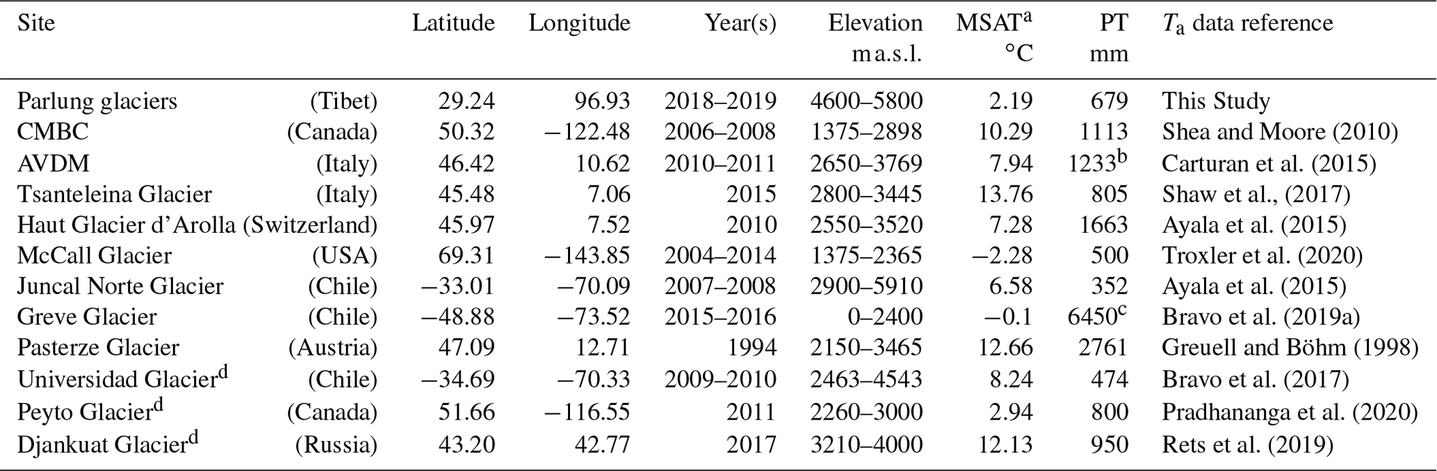
a MSAT corrected from ERA5 grid height to mean elevation of glacier using the environmental lapse rate. b Average for 1979–2009. Precipitation for 2010–2011 was above average at ∼1400 mm (Luca Carutran, personal communication, 2020). c Value taken from Bravo et al. (2019b). d Glaciers where the ELR was used to distribute temperature for calculation. See text for details.
Finally, we group the derived k2 sensitivities of the SM10 approach against the climatology that describes the given glacier(s) location. For this, we consider the mean summer (JJAS or DJFM in the Southern Hemisphere) air temperature (MSAT) and the total annual precipitation for the year(s) of study at each location (Table 2). MSAT is derived from the ERA5 product for the glacier centroid location and corrected to the mean glacier elevation by the ELR. However, total precipitation from ERA5 has been shown to have considerable bias when tested against in situ observations (e.g. Betts et al., 2019), and so we provide the best available value from the relevant literature (Table 2). We note that a full analysis of the local climate is beyond the scope of this work, though we attempted a generalised analysis in order to link any clear differences in the global datasets to climatological influences.
5.1 Variability of on-glacier air temperatures
Figure 3 shows the mean Ta as a function of elevation and flowline distance for the Parlung glaciers for all conditions and for the warmest 10 % of AWS_Off observations (P90). The average of all hours (n=3312) reveals a generally linear relationship with the glacier elevation (Fig. 3a) and flowline distance (Fig. 3b), resulting in a mean on-glacier lapse rate (mean R2 with elevation) equivalent to −3.0 (0.92), −3.7 (0.71) and −4.5 (0.81) for Parlung4, Parlung94 and Parlung390, respectively. For P90 h (n=312), mean Ta demonstrates a poorer fit to elevation and with flowline distance for Parlung4 (mean R2 with elevation = 0.12 and flowline = 0.20) and Parlung 94 (mean R2 with elevation = 0.13 and flowline = 0.09). For the small Parlung390 Glacier, Ta remains strongly related to elevation (R2=0.84) and flowline (R2=0.82) under P90 conditions. The equivalent mean on-glacier lapse rates for P90 h are −2.1, −1.4 and −4.1 . Nevertheless, assuming a 0.5 ∘C uncertainty of the observations for P90 conditions (Fig. 3c and d), the mean of observations still lie along a linear fit line. However, for given hours, the deviation of observations from the linear fit line exceeds 3 ∘C at large flowline distances (>7000 m) on Parlung4. In general, 2018 experienced cooler average temperatures at higher elevations, but in general, there are no marked differences between the two years of observation when comparing on-glacier Ta to glacier elevation or flowline (not shown).
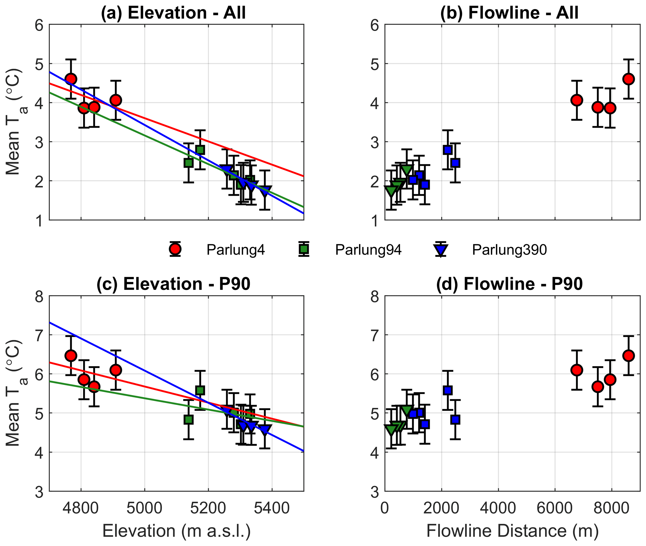
Figure 3The mean Ta against elevation and uncertainty (error bar) for (a) all hours (n=3312) and (c) P90 h (n=312). Panels (b) and (d) are the equivalent plots against flowline distance. Coloured lines show the linear fit against elevation (lapse rate) to each glacier.
5.2 Differences in on- and off-glacier air temperatures
Comparing mean on- and off-glacier Ta at the same elevation reveals the expected behaviour associated with the glacier cooling effect (Carturan et al., 2015) and a greater deviation from the calculated catchment lapse rate temperature for the warmest conditions (P90, Fig. 4), indicating a reduced temperature sensitivity. The mean Ta observed at off-glacier T loggers supports the selection of those stations used for catchment lapse rate calculation (green dots in Fig. 4) that are further from the potential effects of the glacier boundary layer (red markers in Fig. 4). Following Carturan et al. (2015), we suggest a potential non-linear behaviour of lapse rates between AWS_Off and the top of the flowline for Parlung390, though we lack the off-glacier observations above the flowline origin to test this (Fig. 4b). We therefore utilise a piecewise lapse rate at the point of the highest off-glacier lapse rate station (T1390 – red line in Fig. 4) to account for the discrepancy between the estimated and observed Ta at T6390, which is assumed to be near to the flowline origin where temperature sensitivity is theoretically equal to 1 (i.e. where the on-glacier observations are expected to match TaAmb).
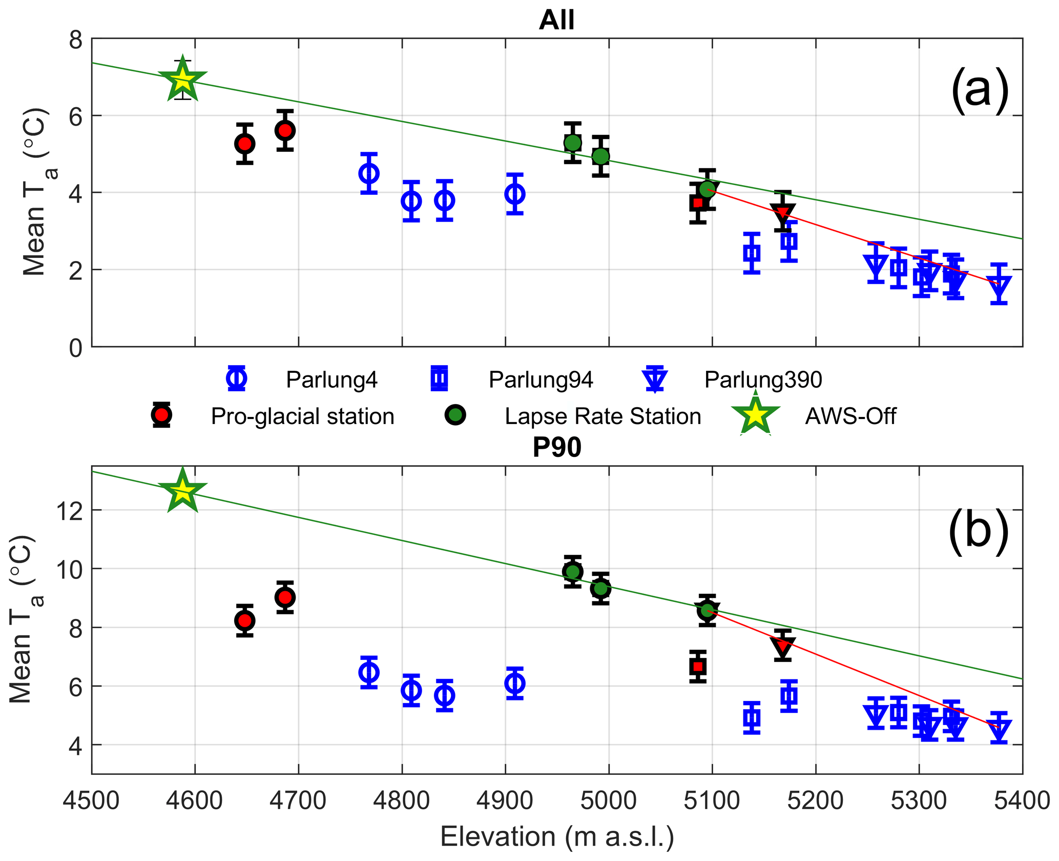
Figure 4The mean Ta against elevation for all hours (a) and P90 h (b), where blue markers are on-glacier T loggers, red markers are pro-glacial T loggers and green circles denote off-glacier T loggers used to construct an hourly variable catchment lapse rate (green line), extrapolated from AWS_Off (star). The red line indicates the piecewise lapse rate above the elevation of T1390 to lapse Ta to the top of the flowline. A 0.5 ∘C uncertainty is shown by the error bar for each station (not applied to the lapse rate for neatness).
Figure 5 presents the hourly differences between TaAmb and observed Ta at each site. The deviation of estimated and observed Ta theoretically begins at a critical temperature threshold, T* (Shea and Moore, 2010), and this effect can be observed at T-logger sites on Parlung94 and Parlung4, particularly those at greater flowline distances. On-glacier Ta and TaAmb align well until the onset of katabatic winds (on Parlung4 and only assumed for the other glaciers due to lack of on-glacier wind observations – Fig. 5). Despite being pro-glacial stations, T14 and T24 reveal a similar albeit weaker effect of the glacier boundary layer, possibly due to larger glacier flowline and extension of the katabatic wind into the pro-glacial area.

Figure 5Estimated (TaAmb) vs. observed Ta at each T-logger location (including off-glacier T loggers). Individual, hourly values are coloured by the observed wind speeds at AWS_On (Parlung4). * denotes stations that are off glacier.
The mean difference of along-flowline Ta and TaAmb using the catchment lapse rate is shown in Fig. 6. For the coolest 10 % of hours at AWS_Off (P10), there is generally minimal difference between TaAmb and observed Ta for the entire dataset. For P90 conditions (Fig. 6a), differences between TaAmb and observed on-glacier temperatures are up to 5.8 ∘C at flowline distances greater than 7000 m. These differences appear to increase beyond 2000 m along the flowline (Parlung94), though significant differences can be witnessed for all glaciers (different symbols in Fig. 6). This is generally associated with drier conditions, and for hours of greater relative humidity (AWS_Off), when conditions are generally cooler, differences are unsurprisingly smaller (Fig. 6b). Considering free-air wind variability provided by ERA5 reanalysis, Ta differences are largest for the dominant south-westerly wind direction (85 % of hours) and when free-air wind speeds are smallest (Fig. 6c and d). However, un-corrected, gridded wind speeds do not appropriately represent the local free-air boundary conditions, and thus the interaction of off-glacier wind speeds and the glacier boundary layer development remains unclear for these glaciers. For all but the coolest ambient temperatures (Fig. 6a), observations at the greatest flowline distances deviate the most from the estimated values. Besides the analyses against individual meteorological variables, the differences are largest for warm/anticyclonic conditions and lowest for cool/cyclonic conditions.

Figure 6The mean and standard deviation (error bars) of hourly Ta differences (TaAmb – observed) along the glacier flowline. Each panel depicts hourly grouping by (a) off-glacier Ta at AWS_Off (P90 is ≥ 10.5 ∘C and P10 is ≤3.5 ∘C), (b) off-glacier RH at AWS_Off (high is >90 % and low is <70 %), (c) wind speed from ERA5 (high is >2.5 m s−1 and low is <0.7 m s−1) and (d) dominant wind direction from ERA5 (south-west wind direction is considered as 180–270∘). Marker shapes show the different glaciers, as in Figs. 3 and 4. X axes are split to improve visibility at low flowline distances.
The differences between TaAmb and on-glacier Ta are highly variable in time, however, and related to the prevailing conditions of a given year (Fig. 7). Considering the maximum daily Ta differences at the on-glacier T logger closest to the terminus of each glacier (Table 1, Fig. 2), we find that Parlung94 and Parlung4 T loggers have similar magnitudes of Ta offsets during the mid-summer months, particularly for 2018 (Fig. 7). These maximum differences are in clear relation to the incoming shortwave radiation recorded at AWS_Off (correlations of 0.44, 0.60 and 0.80 for Parlung390, Parlung94 and Parlung4, respectively), which is indicative of warmer ambient conditions (i.e. P90). For Parlung390 the maximum daily differences are much smaller, though they vary considerably throughout the summer. For 2019, maximum daily Ta offsets on Parlung390 steadily increase during July and August and then fall close to zero in September. The maximum differences for Parlung4 and Parlung94, however, remain sizeable (Fig. 7), perhaps due to the persistence of katabatic winds over a larger flowline distance even under the relatively cooler conditions of September. Because our study period focuses on the core monsoon period (Yang et al., 2011), we do not observe the influence of monsoon arrival or cessation on the Ta variability of the Parlung glaciers.
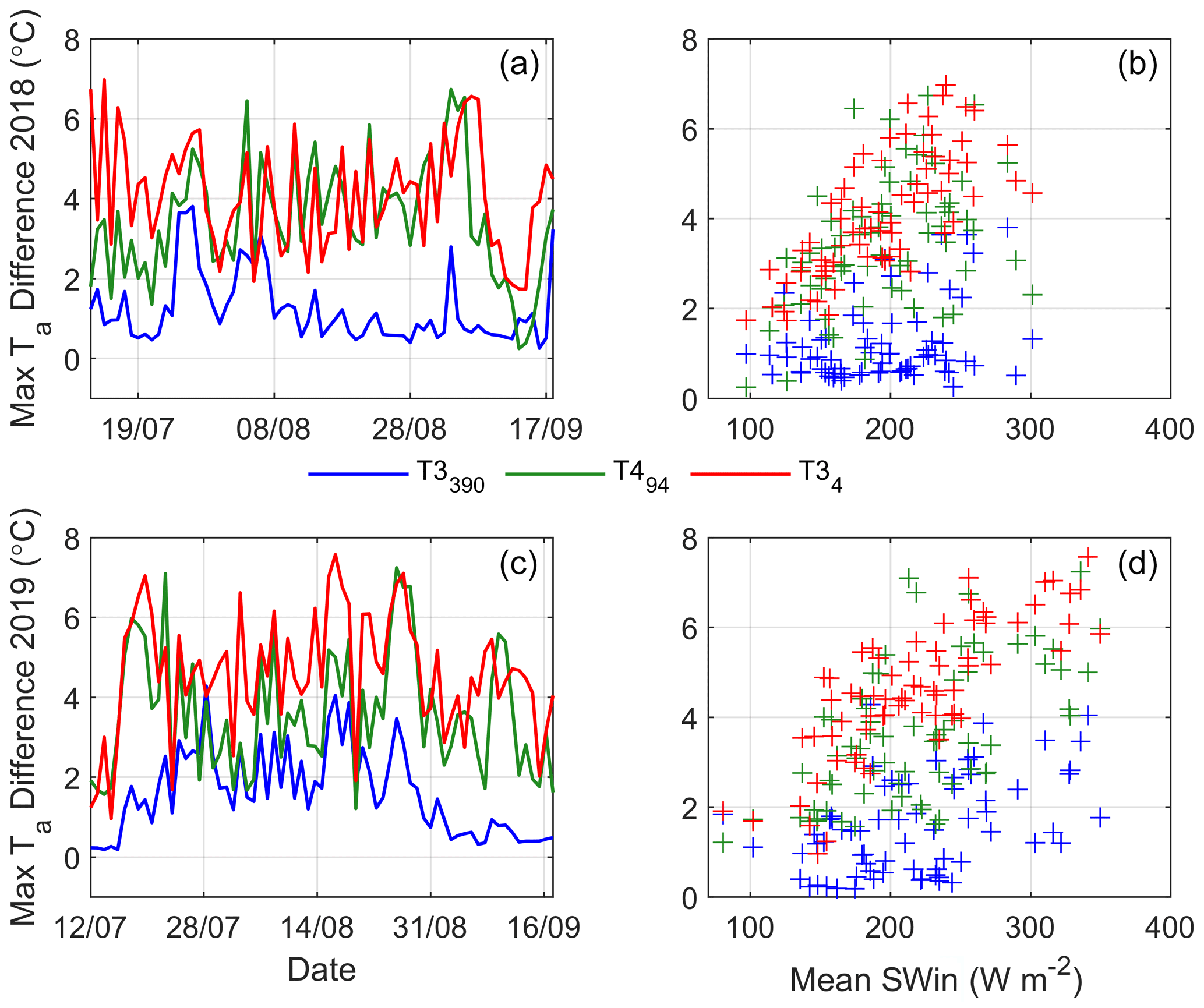
Figure 7Maximum daily Ta differences (TaAmb – observed) at the T logger closest to the terminus on each glacier for 2018 (a, b) and 2019 (c, d). Maximum daily Ta differences are plotted against mean daily incoming shortwave radiation (SWin) at AWS_Off in panels (b) and (d).
5.3 Parameterisation of along-flowline air temperatures
Figure 8 presents the temperature sensitivities of the SM10 approach for the Parlung glaciers and available distributed Ta datasets around the world (Table 2). Comparing the k1 and k2 parameters from Tibet to the parameters of Shea and Moore (2010) from western Canada, a similar behaviour is observable up to ∼2000–3000 m of flowline distance (red and blue symbols). The exponential functions that are fitted to the observations at Parlung glaciers and the original study are distinct (red and blue lines in Fig. 8, Table 3), although within the confidence intervals of each other. Fitting an exponential function for all sites where a down-glacier decrease in temperature sensitivity (k2) is evident (black dashed line in Fig. 8b) clearly misrepresents many of the observations, particularly those at greater flowline distances, balancing the behaviours reported for different sites.
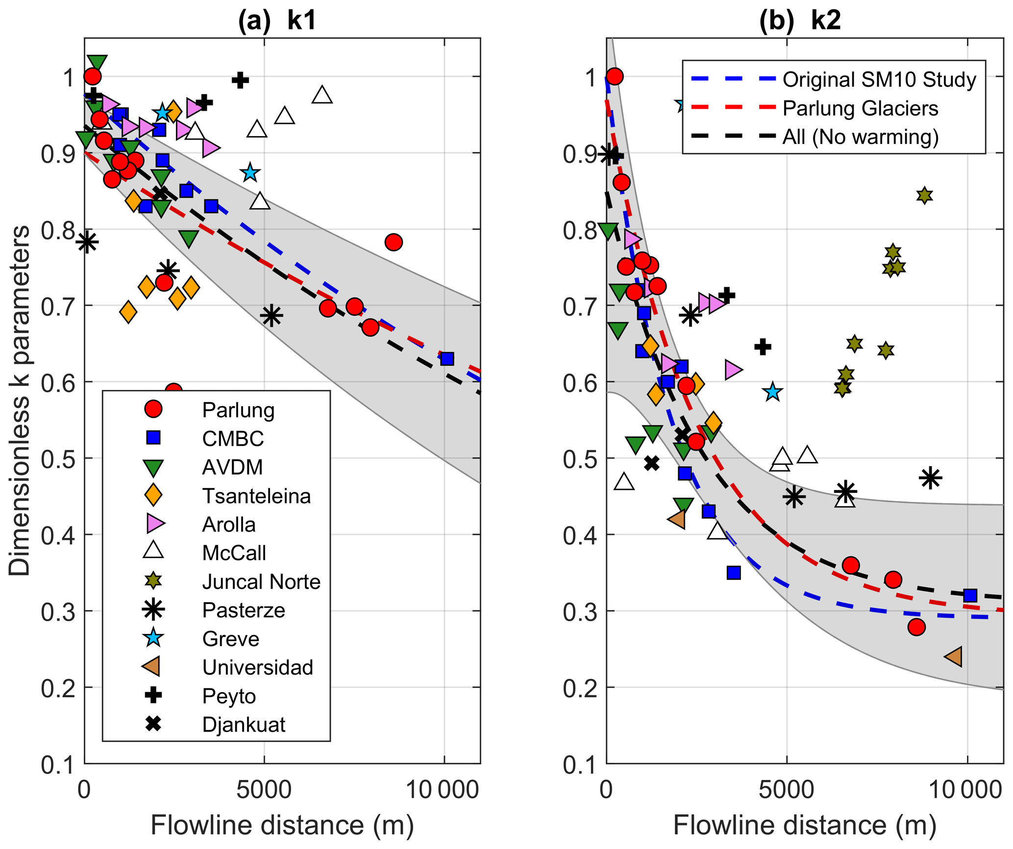
Figure 8The calculated k1 and k2 sensitivities as a function of the flowline distance of each observation on the Parlung glaciers (red circles) and other global datasets (Table 2). The dashed blue and red lines show the fitted exponential parameterisation of Shea and Moore (2010) and this study, respectively. The dashed black line and shaded area denote the equivalent parameterisation for all observations without a large increase in sensitivity on the glacier terminus (warming effect – explicitly excluding data from McCall, Juncal Norte and Djankuat). The shaded area represents the 95 % confidence interval of this fit line.
Table 3The coefficients of the original SM10 model and those fitted to the k1 and k2 sensitivities on the Parlung glaciers and all glaciers where no warming effect was evident (see Fig. 10).
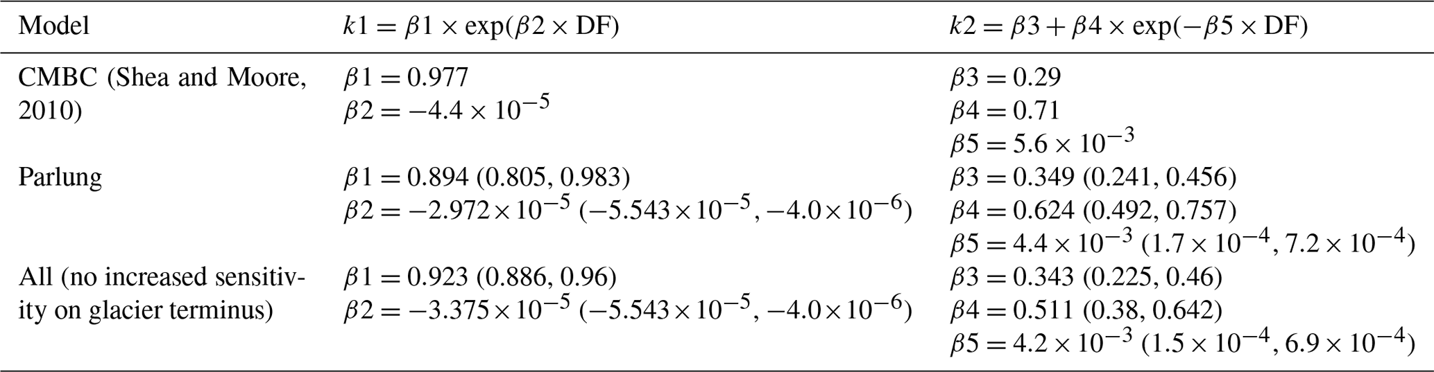
Notably, observations at McCall Glacier, Alaska, relate very well to ambient Ta under cooler conditions, with most k1 values remaining Above the T* threshold, however, the relationship of observed and estimated Ta results in increasing k2 along the flowline, in contradiction to the majority of the other datasets. Nevertheless, these data also confirm the increased temperature sensitivity on the glacier terminus (Troxler et al., 2020) as evident with datasets for Tsanteleina (Shaw et al., 2017), Arolla and Juncal Norte (Ayala et al., 2015). Observations at Parlung4 and Universidad Glacier (Bravo et al., 2017) emphasise the strong decrease in temperature sensitivity at large flowline distances (∼10 000 m) previously only witnessed from one location on Bridge Glacier, Canada (Shea and Moore, 2010). At these stations, changes in on-glacier Ta are less than a third of the equivalent change in TaAmb.
Figure 9 shows the k2 parameters plotted against flowline distance, coloured by rankings of MSAT and precipitation totals (Table 2). The warmest of the investigated sites (during the measurement years) lie closer to the original SM10 exponential function up to ∼4000 m, whereas deviation of the k2 parameters from this line appears larger for the relatively cold sites (Greve, McCall and Peyto – Fig. 9a). The main exception to this is for Juncal Norte, which demonstrates a high and rapidly increasing sensitivity of ambient Ta at the greatest flowline distances.
No clear patterns are visible in relation to mean annual precipitation, though the distinct behaviour at Juncal Norte Glacier corresponds to the driest of the study sites considered (Fig. 9b).
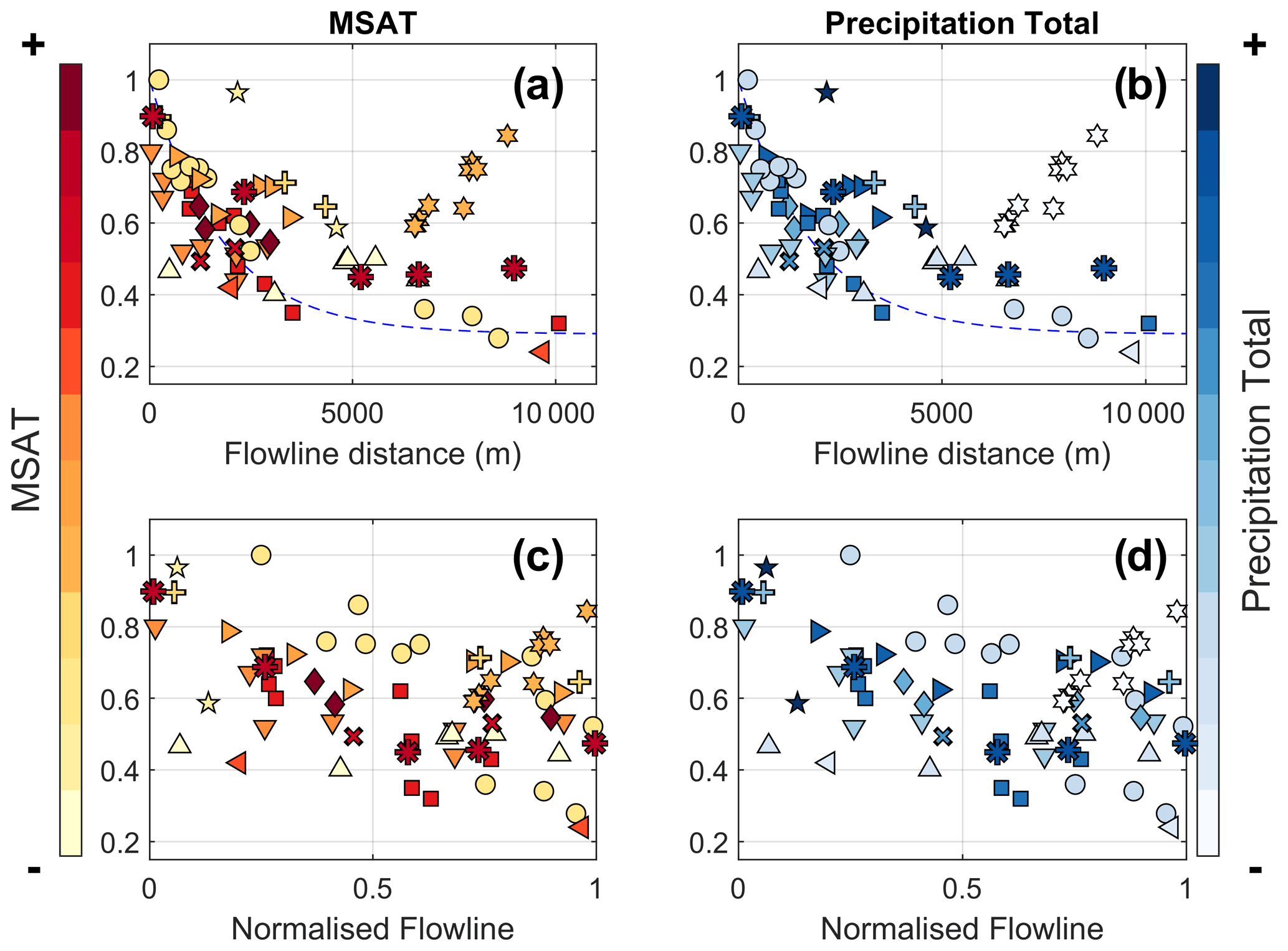
Figure 9The k2 sensitivities as a function of flowline distance (a, b) and a normalised distance, considering the total flowline distance for the year of study (c, d). The individual glaciers of grouped studies (Parlung, CMBC and AVDM) are separated and normalised by the individual glacier length (symbols as in Fig. 8). Glaciers are coloured by rankings of the mean summer air temperatures (MSAT – a and c) and precipitation total (b, d). The original SM10 parameterisation is retained in (a) and (b).
A clear difference between the station observations of Shea and Moore (2010) and Parlung glaciers at large flowline distances (Fig. 8) is the total distance of that station observation from the glacier terminus, which suggests a possible difference in processes occurring between sites. Accordingly, we plot the k2 parameters as a function of the normalised flowline (Fig. 9c and d), adjusted by the total length of glacier for the year(s) of observation (Table 2). The largest flowline distance observation of the entire dataset (Fig. 9a) extends only ∼60 % of the total glacier length (Bridge Glacier – CMBC), neither representing the smallest temperature sensitivity (Fig. 8b), nor an increasing temperature sensitivity witnessed at the terminus of the glacier (and estimated using the ModGB model) by other studies (Ayala et al., 2015; Troxler et al., 2020). We group glaciers by the presence (or absence) of an increasing temperature sensitivity on the terminus in Fig. 10. We find that there is no clear relation between the total length of the glacier and increasing temperature sensitivity, which is seen for both smaller and larger glaciers (Fig. 10b). For those glaciers where a temperature sensitivity increase (a relative ModGB warming effect – Fig. 1a) is evident, it is found only on the lowest 30 % of the glacier terminus (Fig. 10b – vertical dashed line).
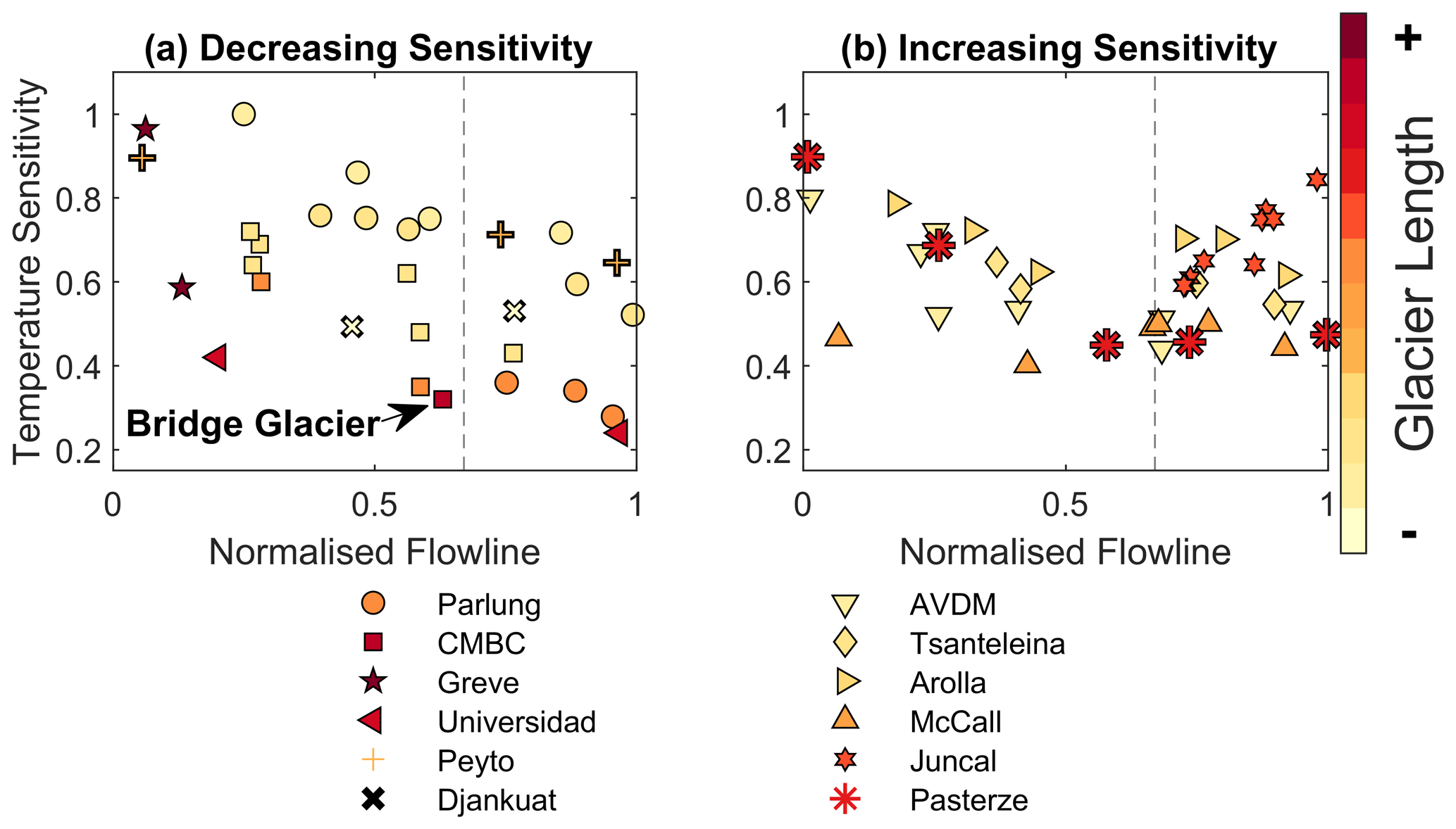
Figure 10The k2 sensitivity along the normalised flowline compared to total glacier length (colour bar). Glaciers have been grouped in two clusters: (a) those with down-glacier decreasing sensitivity, and (b) those with increasing sensitivity towards the glacier terminus.
6.1 Relevance of the findings from Parlung glaciers
Our observations of along-flowline Ta on the glaciers in the Parlung catchment provide more evidence of the spatial variability of the glacier cooling and dampening effect (Oerlemans, 2001; Carturan et al., 2015; Shaw et al., 2017) and highlight the need to appropriately estimate its behaviour for use in glacier energy balance and enhanced temperature index melt models (Petersen and Pellicciotti, 2011; Shaw et al., 2017; Bravo et al., 2019a). It has long been observed that a static lapse rate is inappropriate for characterising the spatio-temporal variability of Ta, both within the KBL (Greuell et al., 1997; Konya et al., 2007; Marshall et al., 2007; Gardner et al., 2009; Petersen and Pellicciotti, 2011) and outside the glacier boundary layer in adjacent valleys (Minder et al., 2010; Immerzeel et al., 2014; Gabbi et al., 2014; Heynen et al., 2016; Jobst et al., 2016). Despite this, the lack of locally available observations often requires modellers to force models with the nearest off-glacier record of Ta and extrapolate it based upon the ELR value as a default. In the case of Tibetan glaciers, model studies have often derived static lapse rates between on- and off-glacier stations (Huintjes et al., 2015) or downscale Ta with a correction factor based upon a single on-glacier location (e.g. Caidong and Sorteberg, 2010; Yang et al., 2013; Zhao et al., 2014). To the authors' knowledge, this is the first time that such detailed information regarding spatio-temporal variations in Ta has been presented for a glacier of the Tibetan Plateau. Because glaciers of the south-eastern Tibetan Plateau have been shown to be particularly susceptible to increases in Ta (Wang et al., 2019), accurately parameterising Ta along glaciers of differing size is highly relevant for present and future melt modelling attempts. This is especially true where glaciers begin to shrink or fragment (Munro and Marosz-Wantuch, 2009; Jiskoot and Mueller, 2012; Carturan et al., 2015) and become more sensitive to ambient air temperatures due to a lack of katabatic boundary layer development (Figs. 6 and 7).
The summer monsoon exerts a strong control on the energy and mass balance of Tibetan glaciers (Yang et al., 2011; Mölg et al., 2012; Zhu et al., 2015). Although our dataset spanned two summers of only the core monsoon period for this region (Yang et al., 2011), we have shown that the sensitivity of the glacier to external temperature changes (shown by on-glacier and ambient Ta differences) has a sizeable temporal variability that can be controlled by the monsoon weather conditions (such as ambient air temperature, humidity and incoming radiation) and can sometimes be independent of the glacier size (Fig. 7). Whilst we cannot determine the impact of monsoon timing and intensity upon the temperature sensitivity of these glaciers with the current dataset, we are able to determine that the observed relationship to flowline distance is consistent with that of other regions of the world (Fig. 8). Future work on Tibetan glaciers should attempt to extend monitoring to the pre-monsoon period to identify if a seasonal onset for the changing glacier temperature sensitivity can be defined and how the monsoon may affect it. Particular focus should be given to understanding the local meteorological conditions for each glacier, as this may explain some of the variability in Ta offset values and why they may sometimes be independent of the along-flowline distance (Fig. 7).
6.2 Parameterising glacier temperature sensitivity
In this study, we discuss the temperature sensitivity of on-glacier Ta based upon observations above a threshold ambient temperature for the onset of katabatic conditions (T*). This sensitivity to ambient temperature during relatively warm conditions, indicated by the k2 parameter of Shea and Moore (2010) (Fig. 1), demonstrates a generally consistent behaviour between the T-logger observations of Parlung glaciers and those where this model had been previously implemented (Shea and Moore, 2010; Carturan et al., 2015). While data from the Parlung catchment provide an important confirmation of the temperature sensitivity for some Tibetan glaciers, further studies of individual glaciers can provide only local parameterisations for temperature sensitivity that may not be applicable to other sites. Accordingly, we have made here one of the first attempts at combining many of the published datasets regarding distributed Ta on mountain glaciers around the world (Table 2) to examine the potential transferability of a model accounting for temperature sensitivity (Fig. 8).
We found a sizeable spread in the temperature sensitivities of Ta for the on-glacier datasets considered, though a consistently rapid decrease in sensitivity along glacier flowlines is found for most sites up until ∼2000–3000 m of distance (Fig. 8b). While localised meteorological and topographic factors likely interact to explain the spread of sensitivities at small flowline distances (Fig. 8b), the results suggest that small glaciers with flow lengths <1000 m would reflect a 0.7–0.8 sensitivity to changes in TaAmb. Beyond this distance, the temperature sensitivities notably follow one of two patterns: a continued albeit less rapid decrease in sensitivity (generally following the model proposed by Shea and Moore, 2010) or a tendency toward increasing sensitivity at the largest flowline distances (in agreement with the ModGB model – Fig. 1a). With reference to the relative Ta differences among only on-glacier observations, these have been termed as down-glacier “cooling” or “warming”, respectively, in many past studies (Ayala et al., 2015; Carturan et al., 2015; Shaw et al., 2017; Troxler et al., 2020). Whilst the former is generally associated with relatively warmer regions of study (Fig. 9), such as the southern Coast Mountains (Shea and Moore, 2010) or Universidad Glacier (Bravo et al., 2017), no strong relationship of the climate setting exists between these sites to explain the magnitude of the temperature sensitivity (i.e. the strength of the glacier cooling and dampening effect) or the observed increases in temperature sensitivity on glacier termini (Ayala et al., 2015; Shaw et al., 2017; Troxler et al., 2020).
Interestingly, we noted that the station with the largest flowline distance used to derive the parameterisation by Shea and Moore (2010) was located at only around 60 % of the total glacier flowline distance (Bridge Glacier – Fig. 10), whereas data presented by other studies provided observations up to the glacier terminus (Greuell and Böhm, 1998; Ayala et al., 2015; Shaw et al., 2017; Troxler et al., 2020), therefore potentially parameterising different effects of the glacier boundary layer. It has been suggested that observations at large flowline distances (such as those on Parlung4 or Bridge Glacier) represent a segment of the boundary layer where the near-surface layer becomes highly insensitive to the ambient free-air temperature fluctuations (point 3 in Fig. 1a and d). This phenomenon has been shown to be sustained over large fetch distances by an increasing depth of the glacier wind layer (van den Broeke, 1997; Greuell and Böhm, 1998; Shea and Moore, 2010; Jiskoot and Mueller, 2012). However, as air parcels travel down glacier toward the glacier terminus (point 4 in Fig. 1a and d), they potentially encounter warm-air entrainment due to a divergent boundary layer (Munro, 2006), up-valley winds (Pellicciotti et al., 2008; Oerlemans, 2010; Petersen and Pellicciotti, 2011), large changes in surface slope and the dominance of adiabatic heating over sensible heat losses (Greuell and Böhm, 1998), or heating from debris-covered ice at the terminus (Brock et al., 2010; Shaw et al., 2016; Steiner and Pellicciotti, 2016; Bonekamp et al., 2020). These are effects of the glacier boundary layer that the ModGB model was designed to account for, though we did not explicitly test this within our study due to a requirement for more data and a greater number of parameters and assumptions (Shaw et al., 2017). The strength of this so called along-glacier warming effect could therefore be governed by local topography (adjusting the boundary layer convergence or divergence) or the total glacier flowline distance and the large fetch of a cool air parcel overcoming the competing effect of warm, up-valley winds (Fig. 1d – as seen at T24 in Fig. 5).
By grouping glaciers by the presence of the observed increase in temperature sensitivity and normalising the flowline distance of the observations by the total flowline for each glacier, we identify that the relative increases in temperature sensitivity begin at ∼70 % of the total flowline distance (Fig. 10). A smaller temperature sensitivity can be observed for larger glaciers (Fig. 10a), which is consistent with the development of the KBL over a large fetch (Greuell and Böhm, 1998; Shea and Moore, 2010), though the length itself indicates nothing clear about why greater temperature sensitivity exists for some glacier termini (Fig. 10b).
The clear outlier of these datasets is Juncal Norte Glacier in Chile (Fig. 8b). It is interesting to note that Juncal Norte is the only reported case in the literature on Ta variability where the warmest hours of the afternoon correspond to the dominance of an up-valley, off-glacier wind (Pellicciotti et al., 2008; Petersen and Pellicciotti, 2011). Counter to the typical role of the dominant, down-glacier wind layer for these warmest afternoon hours (Greuell et al., 1997; Greuell and Böhm, 1998; Strasser et al., 2004; Jiskoot and Mueller, 2012; Shaw et al., 2017; Troxler et al., 2020), up-valley winds on Juncal Norte seemingly erode the along-flowline reduction in temperature sensitivity (along-flowline cooling) up to a distance along the flowline where it is theoretically at its maximum (point 3 in Fig. 1). Evidence from other glaciers suggest that this point is close to upper observations for Juncal Norte at ∼70 % of the total flowline (Fig. 10b), though further observations on Juncal Norte Glacier would be required to test this.
Finally, the extent to which a glacier terminus is constrained by high valley slopes may be an additional explanatory factor for the occurrence of increasing temperature sensitivities on some glaciers (Fig. 10). While this may limit the suggested boundary layer divergence (Munro, 2006), it may equally promote greater warming due longwave emission from valley slopes (e.g. Strasser et al., 2004; Ayala et al., 2015). We calculated the terminus widthlength ratio of each glacier and compared it to the presence of increasing temperature sensitivity on the terminus (Fig. S4 in the Supplement), revealing a potential relationship between the two. However, given the available data for this study and the unknown extent to which longwave emission may affect a fast-moving air parcel (Ayala et al., 2015), a dedicated study would be required to further address this hypothesis.
6.3 Future directions for researching air temperatures on glaciers
A limitation of our work is the dependency of the derived global temperature sensitivities (Fig. 8b) to the available off-glacier data and the published lapse rates to extrapolate them to the relevant elevations on glacier. In our case, we are able to identify a potentially non-linear lapse rate of TaAmb for the highest elevations over Parlung94 and Parlung390 (Fig. 4). Although we cannot confirm this without off-glacier observations above the top of the flowline (Carturan et al., 2015), we are able to well constrain ambient air temperature distribution using hourly observations at several off-glacier locations to derive the best possible catchment lapse rate. For other datasets (Table 2), we rely upon the available off-glacier data and lapse rates that are not derived in a consistent manner. The derivation of flowline distances from the DEM is also not consistent between the prior studies (Shea and Moore, 2010; Carturan et al., 2015; Shaw et al., 2017; Bravo et al., 2019a; Troxler et al., 2020) and may hold some small influence on the derived parameterisations (Table 3), particularly at lateral locations on the glacier (not explored here), which can be subject to different micro-meteorological effects (van de Wal et al., 1992; Hannah et al., 2000; Shaw et al., 2017). Equally, the uncertainty of the actual observations (e.g. Sect. 3.2) is hard to clearly define due the variable instrumentation (sensors and radiation shielding), on-glacier location, and local topographic and micro-meteorological effects of each study site (Table 2). Because our study, and many similar studies of this kind, did not have artificially ventilated radiation shields available, the uncertainty of the measured Ta is difficult to quantify. We consider this to be less problematic at large flowline distances, where good ventilation to the sensors is often provided by the glacier katabatic wind layer even under warm conditions. However, at short flowline distances in the glacier accumulation zones, uncertainty of both the on-glacier observations and ambient Ta extrapolation is larger. Artificially ventilated radiation shields are not commonplace in glaciological research due to the additional power demands that often cannot be met though would be strongly encouraged for further research into the temperature sensitivity of mountain glaciers. Further work on a unified model of estimating Ta should need to address these issues, perhaps with further dedicated analyses.
In our study, we apply the parameterisation of Carturan et al. (2015) to derive along-flowline values of the theoretical onset of the KBL (T*). While these values appear appropriate for our case studies (based upon manual inspection), they were derived for a smaller sample size of total observations. We experimented with a static T* value of 5 ∘C in order to test the sensitivity of our analysis to the assumptions of T*, though we found negligible sensitivity of derived k2 on T* (not shown). Similarly, a sensitivity to the choice of constant lapse rate for those sites without available lapse rate information (Table 2) proved to have only a small influence on the derived k1 and k2 values.
Finally, in this study we assess temperature sensitivity based upon ambient air temperatures above the T* threshold. This is partly different from the “climatic sensitivity” presented by earlier works (Greuell et al., 1997; Greuell and Böhm, 1998; Oerlemans, 2001, 2010), which considered an all-hour temperature sensitivity value (i.e. not thresholding sensitivities by katabatic wind onset – Fig. 1b). However, ignoring the differences in temperature sensitivity before and after the onset of the KBL (Figs. 1c and 5) is arguably an over-simplification and does not enable one to correctly describe the observed behaviours (Shea and Moore, 2010; Jiskoot and Mueller, 2012). Accordingly, we caution somewhat the direct comparison of the temperature sensitivity presented here and the “climatic sensitivity” of previous works.
We consider the SM10 approach and the use of k2 to be an appropriate indicator of temperature sensitivity for mountain glaciers in future work of this type. This approach is an easily adaptable method for calculating glacier temperature sensitivity and thus estimating on-glacier Ta. However, the competing effects of glacier katabatic and up-valley winds/debris or valley warming need to be incorporated to address the challenges that less simplistic methods (i.e. ModGB) were designed for.
Based upon the findings of this work, we recommend that future research (i) attempt to standardise, where possible, the measurement and comparison of off- and on-glacier air temperature, exploring the use of artificially ventilated radiation shields that are less prone to heating errors (Georges and Kaser, 2002; Carturan et al., 2015), (ii) instrument glaciers of varying size in the same catchment to explore the relative importance of glacier size and local meteorological conditions (Fig. 7), and (iii) model the detailed interactions of air flows on glacier termini using, for example, large eddy simulations (Sauter and Galos, 2016; Bonekamp et al., 2020) in order to identify possible drivers of the observed increase in temperature sensitivity for certain glacier areas (point 4 in Fig. 1).
We presented a new dataset of distributed on-glacier air temperatures for three glaciers of different size in the south-east Tibetan Plateau during two summers (July–September). We analysed the along-flowline air temperature distribution for all three glaciers and compared them to the estimated ambient temperatures derived from several local off-glacier stations. Using this information, we parameterised the along-flowline temperature sensitivities of these glaciers using the method proposed by Shea and Moore (2010) and presented the results in the context of several available distributed on-glacier datasets. The key findings of this work are the following.
-
For our Tibetan case study, on-glacier air temperatures at short flowline distances display a high temperature sensitivity (i.e. demonstrate a relationship with off-glacier air temperature that is close to 1). We therefore confirm earlier evidence regarding the high temperature sensitivity of high-elevation, small glaciers (flowline distances <1000 m) to external climate and thus future warming.
-
The largest differences between observed on-glacier and estimated off-glacier air temperatures are found for the warmest off-glacier hours during drier, clear-sky conditions of the summer monsoon period.
-
Above the established onset of the katabatic boundary layer, temperature sensitivity to ambient temperature decreases rapidly up to ∼2000–3000 m along the glacier flowline. Beyond this distance, both the Tibetan glaciers and other datasets of the literature show a slower decrease in temperature sensitivity.
-
A parameterisation for the temperature sensitivity of the Tibetan study glaciers implies a similar boundary layer effect compared to the existing parameterisation of Shea and Moore (2010). The climatology of a given region may influence the magnitude of the glacier's temperature sensitivity, though no clear relationships with the climatology of the glacier sites are found, thus suggesting the stronger role of local meteorological or topographic effects on the along-flowline pattern of Ta variability.
-
The terminus of some glaciers is associated with other warm-air processes, possibly due to boundary layer divergence, warm up-valley winds, large glacier slope changes or debris cover/valley heating. We find that these effects are evident only beyond ∼70 % of the total glacier flowline distance, although further work is required to explain this behaviour. A better understanding of temperature variability for this lower 30 % is highly important as this part of the glacier is most affected by ablation.
In summarising the findings from all available distributed on-glacier datasets to date, we identify some key directions for future work on this subject. This includes comparing local influences of glacier size and micro-meteorology and standardising measurement practices, where possible, to enable the construction of a generalised model for on-glacier air temperature estimation.
Calculated flowlines and temperature sensitivities are available at the following Zenodo repository: https://doi.org/10.5281/zenodo.3937777 (Shaw et al., 2020).
The supplement related to this article is available online at: https://doi.org/10.5194/tc-15-595-2021-supplement.
TES and WY discussed and designed the research plan with Parlung data provided by WY and CZ. Additional data and analysis were provided by AA and CB. TES wrote the manuscript with scientific input from all co-authors.
The authors declare that they have no conflicting interests.
Funding for the instrumentation of the Parlung catchment was provided by an NSFC project (91647205 and 41961134035) and Newton Advanced Fellowship (NA170325). This project has received funding from the European Research Council (ERC) under the European Union's Horizon 2020 research and innovation programme grant agreement no. 772751, RAVEN (Rapid mass losses of debris-covered glaciers in High Mountain Asia). Álvaro Ayala acknowledges support from a FONDECYT project (number 3190732) and Claudio Bravo from the ANID Be- cas Chile PhD scholarship program. The authors kindly acknowledge the sharing of global datasets or parameters provided to aid this analysis, explicitly Matt Nolan (McCall Glacier), Paul Smeets and IMAU, Utrecht (Pasterze Glacier), DGA, Chile (Universidad Glacier and Greve Glacier) and Luca Carturan (AVDM, Italy). The Peyto Glacier data used this paper were provided by John Pomeroy, as well as Dhiraj Pradhananga of the University of Saskatchewan Centre for Hydrology through the Global Water Futures (GWF) programme. Elke Ludewig is thanked for the provision of off-glacier temperature records at Sonnblick station, Austria. Additionally we recognise the hard work involved in obtaining and sharing all of the datasets acquired and the acknowledgements of those works. Scientific editor Tobias Sauter, Luca Carturan and one anonymous reviewer are thanked for their insightful and constructive comments that have improved the quality of the manuscript.
This project has received funding from the European Research Council (ERC) under the European Union's Horizon 2020 research and innovation programme grant agreement no. 772751, RAVEN (Rapid mass losses of debris-covered glaciers in High Mountain Asia).
This paper was edited by Tobias Sauter and reviewed by Luca Carturan and one anonymous referee.
ASF DAAC: ALOS PALSAR_Radiometric_Terrain_Corrected_low_res, Includes Material © JAXA/METI 2007, Accessed through ASF DAAC 20 March 2020, https://doi.org/10.5067/JBYK3J6HFSVF, 2020.
Arnold, N. S., Rees, W. G., Hodson, A. J., and Kohler, J.: Topographic controls on the surface energy balance of a high Arctic valley glacier, J. Geophys. Res., 111, F02011, https://doi.org/10.1029/2005JF000426, 2006.
Ayala, A., Pellicciotti, F., and Shea, J.: Modeling 2m air temperatures over mountain glaciers: Exploring the influence of katabatic cooling and external warming, J. Geophys. Res.-Atmos, 120, 1–19, https://doi.org/10.1002/2015JD023137, 2015.
Betts, A. K., Chan, D. Z., and Desjardins, R. L.: Near-Surface Biases in ERA5 Over the Canadian Prairies, Front. Environ. Sci., 7, 129, https://doi.org/10.3389/fenvs.2019.00129, 2019.
Bonekamp, P. N. J., van Heerwaarden, C. C., Steiner, J. F., and Immerzeel, W. W.: Using 3D turbulence-resolving simulations to understand the impact of surface properties on the energy balance of a debris-covered glacier, The Cryosphere, 14, 1611–1632, https://doi.org/10.5194/tc-14-1611-2020, 2020.
Bravo, C., Loriaux, T., Rivera, A., and Brock, B. W.: Assessing glacier melt contribution to streamflow at Universidad Glacier, central Andes of Chile, Hydrol. Earth Syst. Sci., 21, 3249–3266, https://doi.org/10.5194/hess-21-3249-2017, 2017.
Bravo, C., Quincey, D. J., Ross, A. N., Rivera, A., Brock, B. W., Miles, E., and Silva, A.: Air Temperature Characteristics, Distribution, and Impact on Modeled Ablation for the South Patagonia Ice field, J. Geophys. Res.-Atmos., 124, 907–925, https://doi.org/10.1029/2018JD028857, 2019a.
Bravo, C., Bozkurt, D., Gonzalez-reyes, Á., Quincey, D. J., Ross, A. N., Farias-Barahona, D., and Rojas, M.: Assessing Snow Accumulation Patterns and Changes on the Patagonian Icefields, Front. Environ. Sci., 7, 1–18, https://doi.org/10.3389/fenvs.2019.00030, 2019b.
Brock, B. W., Mihalcea, C., Kirkbride, M. P., Diolaiuti, G., Cutler, M. E. J., and Smiraglia, C.: Meteorology and surface energy fluxes in the 2005–2007 ablation seasons at the Miage debris-covered glacier, Mont Blanc Massif, Italian Alps, J. Geophys. Res, 115, D09106, https://doi.org/10.1029/2009JD013224, 2010.
Caidong, C. and Sorteberg, A.: Modelled mass balance of Xibu glacier, Tibetan Plateau: Sensitivity to climate change, J. Glaciol, 56, 235–248, https://doi.org/10.3189/002214310791968467, 2010.
Carturan, L., Cazorzi, F., De Blasi, F., and Dalla Fontana, G.: Air temperature variability over three glaciers in the Ortles–Cevedale (Italian Alps): effects of glacier fragmentation, comparison of calculation methods, and impacts on mass balance modeling, The Cryosphere, 9, 1129–1146, https://doi.org/10.5194/tc-9-1129-2015, 2015.
Copernicus Climate Change Service (C3S): ERA5: Fifth generation of ECMWF atmospheric reanalyses of the global climate, Copernicus Climate Change Service Climate Data Store (CDS), available at: https://cds.climate.copernicus.eu/cdsapp#!/home (last access: 5 May 2020), 2017.
Ding, B., Yang, K., Yang, W., He, X., Chen, Y., Lazhu, Guo, X., Wang, L., Wu, H., and Yao, T.: Development of a Water and Enthalpy Budget-based Glacier mass balance Model (WEB-GM) and its preliminary validation, Water Resour. Res., 53, 3146–3178, https://doi.org/10.1002/2016WR018865, 2017.
Gabbi, J., Carenzo, M., Pellicciotti, F., Bauder, A., and Funk, M.: A comparison of empirical and physically based glacier surface melt models for long-term simulations of glacier response, J. Glaciol, 60, 1140–1154, https://doi.org/10.3189/2014JoG14J011, 2014.
Gardner, A. S., Sharp, M. J., Koerner, R. M., Labine, C., Boon, S., Marshall, S. J., Burgess, D. O., and Lewis, D.: Near-Surface Temperature Lapse Rates over Arctic Glaciers and Their Implications for Temperature Downscaling, J. Climate, 22, 4281–4298, https://doi.org/10.1175/2009JCLI2845.1, 2009.
Georges, C. and Kaser, G.: Ventilated and unventilated air temperature measurements for glacier-climate studies on a tropical high mountain site, J. Geophys. Res., 107, 4775, https://doi.org/10.1029/2002JD002503, 2002.
Greuell, W. and Böhm, R.: 2 m temperatures along melting mid-latitude glaciers, and implications for the sensitivity of the mass balance to variations in temperature, J. Glaciol, 44, 9–20, 1998.
Greuell, W., Knap, W. H., and Smeets, P. C.: Elevational changes in meteorological variables along a midlatitude glacier during summer, J. Geophys. Res., 102, 25941, https://doi.org/10.1029/97JD02083, 1997.
Hannah, D. M., Gurnell, A. M., and McGregor, G. R.: Spatio-temporal variation in microclimate, the surface energy balance and ablation over a cirque glacier, Int. J. Climatol., 20, 733–758, https://doi.org/10.1002/1097-0088(20000615)20:7<733::AID-JOC490>3.0.CO;2-F, 2000.
Heynen, M., Miles, E., Ragettli, S., Buri, P., Immerzeel, W., and Pellicciotti, F.: Air temperature variability in a high elevation Himalayan catchment, Ann. Glaciol., 57, 212–222, https://doi.org/10.3189/2016AoG71A076, 2016.
Huintjes, E., Sauter, T., Schröter, B., Maussion, F., Yang, W., Kropácek, J., Buchroithner, M., Scherer, D., Kang, S., and Schneider, C.: Evaluation of a Coupled Snow and Energy Balance Model for Zhadang Glacier, Tibetan Plateau, Using Glaciological Measurements and Time-Lapse Photography, Arct. Antarct. Alp. Res., 47, 573–590, https://doi.org/10.1657/AAAR0014-073, 2015.
Immerzeel, W. W., Petersen, L., Ragettli, S., and Pellicciotti, F.: The importance of observed gradients of air temperature and precipitation for modeling runoff from a glacierized watershed, Water Resour. Res., 50, 2212–2226, https://doi.org/10.1002/2013WR014506, 2014.
Jiskoot, H. and Mueller, M. S.: Glacier fragmentation effects on surface energy balance and runoff: field measurements and distributed modelling, Hydrol. Process., 26, 1861–1875, https://doi.org/10.1002/hyp.9288, 2012.
Jobst, A. M., Kingston, D. G., Cullen, N. J., and Sirguey, P.: Combining thin-plate spline interpolation with a lapse rate model to produce daily air temperature estimates in a data-sparse alpine catchment, Int. J. Climatol., 37, 214–229, https://doi.org/10.1002/joc.4699, 2016.
Konya, K., Hock, R., and Naruse, R. Temperature lapse rates and surface energy balance at Storglaciären, northern Sweden, Glacier Mass Balance and Meltwater Discharge, 186–194, 2007.
Marshall, S. J., Sharp, M. J., Burgess, D. O., and Anslow, F. S.: Near-surface-temperature lapse rates on the Prince of Wales Icefield, Ellesmere Island, Canada: implications for regional downscaling of temperature, Int. J. Climatol., 27, 1549–1555, https://doi.org/10.1002/joc.1396, 2007.
Maurer, J. M., Schaefer, J. M., Rupper, S., and Corley, A.: Acceleration of ice loss across the Himalayas over the past 40 years, Sci. Adv., 5, 1–12, 2019.
Minder, J. R., Mote, P. W., and Lundquist, J. D.: Surface temperature lapse rates over complex terrain: Lessons from the Cascade Mountains, J. Geophys. Res., 115, D14122, https://doi.org/10.1029/2009JD013493, 2010.
Mölg, T., Maussion, F., Yang, W., and Scherer, D.: The footprint of Asian monsoon dynamics in the mass and energy balance of a Tibetan glacier, The Cryosphere, 6, 1445–1461, https://doi.org/10.5194/tc-6-1445-2012, 2012.
Munro, D. S.: Linking the weather to glacier hydrology and mass balance at Peyto glacier, Peyto Glacier: One Century of Science, National Hydrology Research Institute, Science Report #8, 2006.
Munro, D. S. and Marosz-Wantuch, M.: Modeling Ablation on Place Glacier, British Columbia, from Glacier and Off-glacier Data Sets, Arct. Antarct. Alp. Res., 41, 246–256, https://doi.org/10.1657/1938-4246-41.2.246, 2009.
Nolin, A. W., Phillippe, J., Jefferson, A., and Lewis, S. L.: Present-day and future contributions of glacier runoff to summertime flows in a Pacific Northwest watershed: Implications for water resources, Water Resour. Res., ., 46, W12509, https://doi.org/10.1029/2009WR008968, 2010.
Oerlemans, B. J. and Grisogono, B.: Glacier winds and parameterisation of the related surface heat fluxes, Tellus, 54, 440–452, 2002.
Oerlemans, J.: Glaciers and Climate Change, A. A. Balkema Publishers, xii, 148 pp., 2001.
Oerlemans, J.: The microclimate of valley glaciers, Utrecht Publishing and Archiving Services, Universiteitsbibliotheek, Utrecht, 2010.
Pellicciotti, F., Brock, B. W., Strasser, U., Burlando, P., Funk, M., and Corripio, J. G.: An enhanced temperature-index glacier melt model including the shortwave radiation balance: development and testing for Haut Glacier d'Arolla, Switzerland, J. Glaciol., 51, 573–587, 2005.
Pellicciotti, F., Helbing, J., Rivera, A., Favier, V., Corripio, J. G., Araos, J., Sicart, J.-E., and Carenzo, M.: A study of the energy balance and melt regime on Juncal Norte Glacier, semi-arid Andes of central Chile, using melt models of different complexity, Hydrol. Process., 22, 3980–3997, https://doi.org/10.1002/hyp.7085, 2008.
Pellicciotti, F., Ragettli, S., Carenzo, M., and McPhee, J.: Changes of glaciers in the Andes of Chile and priorities for future work, Sci. Total Environ., 493C, 1197–1210, https://doi.org/10.1016/j.scitotenv.2013.10.055, 2014.
Petersen, L. and Pellicciotti, F.: Spatial and temporal variability of air temperature on a melting glacier: Atmospheric controls, extrapolation methods and their effect on melt modeling, Juncal Norte Glacier, Chile, J. Geophys. Res., 116, D23109, https://doi.org/10.1029/2011JD015842, 2011.
Petersen, L., Pellicciotti, F., Juszak, I., Carenzo, M., and Brock, B. W.: Suitability of a constant air temperature lapse rate over an Alpine glacier: testing the Greuell and Böhm model as an alternative, Ann. Glaciol., 54, 120–130, https://doi.org/10.3189/2013AoG63A477, 2013.
Pradhananga, D., Pomeroy, J. W., Aubry-Wake, C., Munro, D. S., Shea, J., Demuth, M. N., Kirat, N. H., Menounos, B., and Mukherjee, K.: Hydrometeorological, glaciological and geospatial research data from the Peyto Glacier Research Basin in the Canadian Rockies, Earth Syst. Sci. Data Discuss. [preprint], https://doi.org/10.5194/essd-2020-219, in review, 2020.
Ragettli, S., Immerzeel, W. W., and Pellicciotti, F.: Contrasting climate change impact on river flows from high-altitude catchments in the Himalayan and Andes Mountains, P. Natl. Acad. Sci. USA, 113, 9222–9227, https://doi.org/10.1073/pnas.1606526113, 2016.
Rets, E. P., Popovnin, V. V., Toropov, P. A., Smirnov, A. M., Tokarev, I. V., Chizhova, J. N., Budantseva, N. A., Vasil'chuk, Y. K., Kireeva, M. B., Ekaykin, A. A., Veres, A. N., Aleynikov, A. A., Frolova, N. L., Tsyplenkov, A. S., Poliukhov, A. A., Chalov, S. R., Aleshina, M. A., and Kornilova, E. D.: Djankuat glacier station in the North Caucasus, Russia: a database of glaciological, hydrological, and meteorological observations and stable isotope sampling results during 2007–2017, Earth Syst. Sci. Data, 11, 1463–1481, https://doi.org/10.5194/essd-11-1463-2019, 2019.
Sauter, T. and Galos, S. P.: Effects of local advection on the spatial sensible heat flux variation on a mountain glacier, The Cryosphere, 10, 2887–2905, https://doi.org/10.5194/tc-10-2887-2016, 2016.
Schwanghart, W. and Kuhn, N, J.: TopoToolbox: A set of Matlab functions for topographic analysis, Environ. Modell. Softw., 25, 770–781, https://doi.org/10.1016/j.envsoft.2009.12.002, 2010.
Shaw, T., Brock, B., Fyffe, C., Pellicciotti, F., Rutter, N., and Diotri, F.: Air temperature distribution and energy balance modelling of a debris-covered glacier, J. Glaciol., 62, 185–198, https://doi.org/10.1017//jog.2016.31, 2016.
Shaw, T. E., Brock, B. W., Ayala, A., Rutter, N., and Pellicciotti, F.: Centreline and cross-glacier air temperature variability on an Alpine glacier: assessing temperature distribution methods and their influence on melt model calculations, J. Glaciol., 63, 1–16, https://doi.org/10.1017/jog.2017.65, 2017.
Shaw, T. E., Yang, W., Ayala, Á., Bravo, C., Zhao, C., and Pellicciotti. F.: Temperature sensitivity of mountain glaciers [Data set], Zenodo, https://doi.org/10.5281/zenodo.3937777, 2020.
Shea, J. M. and Moore, R. D.: Prediction of spatially distributed regional-scale fields of air temperature and vapor pressure over mountain glaciers, J. Geophys. Res., 115, D23107, https://doi.org/10.1029/2010JD014351, 2010.
Steiner, J. F. and Pellicciotti, F.: Variability of air temperature over a debris-covered glacier in the Nepalese Himalaya, Ann. Glaciol., 57, 295–307, https://doi.org/10.3189/2016AoG71A066, 2016.
Strasser, U., Corripio, J. G., Pellicciotti, F., Burlando, P., Brock, B. W., and Funk, M.: Spatial and temporal variability of meteorological variables at Haut Glacier d'Arolla (Switzerland) during the ablation season 2001: Measurements and simulations, J. Geophys. Res., 109, D03103, https://doi.org/10.1029/2003JD003973, 2004.
Troxler, P., Ayala, Á., Shaw, T. E., Nolan, M., Brock, B. W., and Pellicciotti, F.: Modelling spatial patterns of near-surface air temperature over a decade of melt seasons on McCall Glacier, Alaska. J. Glaciol, 66, 386–400, https://doi.org/10.1017/jog.2020.12, 2020.
van de Wal, R. S. W., Oerlemans, J., and Van Der Hage, J. C.: A study of ablation variations on the tongue of Hintereisferner, Austrian Alps, J. Glaciol., 38, 319–324, 1992.
van den Broeke, M. R.: Momentum, Heat, and Moisture Budgets of the Katabatic Wind Layer over a Midlatitude Glacier in Summer, J. Appl. Meteorol., 36, 763–774, 1997.
Wang, R., Liu, S., Shangguan, D., Radić, V., and Y, Z.: Spatial Heterogeneity in Glacier Mass-Balance, Water, 11, 1–21, https://doi.org/10.3390/w11040776, 2019.
Yang, W., Guo, X., Yao, T., Yang, K., Zhao, L., Li, S., and Zhu, M.: Summertime surface energy budget and ablation modeling in the ablation zone of a maritime Tibetan glacier, J. Geophys. Res.-Atmos., 116, 1–11, https://doi.org/10.1029/2010JD015183, 2011.
Yang, W., Yao, T., Guo, X., Zhu, M., Li, S., and Kattel, D. B.: Mass balance of a maritime glacier on the southeast Tibetan Plateau and its temperature sensitivity, J. Geophys. Res.-Atmos., 118, 9579–9594, https://doi.org/10.1002/jgrd.50760, 2013.
Zhao, L., Tian, L., Zwinger, T., Ding, R., Zong, J., Ye, Q., and Moore, J. C.: Numerical simulations of Gurenhekou glacier on the Tibetan Plateau, J. Glaciol., 60, 71–82, https://doi.org/10.3189/2014JoG13J126, 2014.
Zhu, M., Yao, T., Yang, W., Maussion, F., Huintjes, E., and Li, S.: Energy- and mass-balance comparison between Zhadang and Parlung No. 4 glaciers on the Tibetan Plateau, J. Glaciol., 61, 595–607, https://doi.org/10.3189/2015JoG14J206, 2015.