the Creative Commons Attribution 4.0 License.
the Creative Commons Attribution 4.0 License.
 | 25 Oct 2021
The role of sublimation as a driver of climate signals in the water isotope content of surface snow: laboratory and field experimental results
Abigail G. Hughes
Sonja Wahl
Tyler R. Jones
Alexandra Zuhr
Maria Hörhold
James W. C. White
Hans Christian Steen-Larsen
Ice core water isotope records from Greenland and Antarctica are a valuable proxy for paleoclimate reconstruction, yet the processes influencing the climate signal stored in the isotopic composition of the snow are being challenged and revisited. Apart from precipitation input, post-depositional processes such as wind-driven redistribution and vapor–snow exchange processes at and below the surface are hypothesized to contribute to the isotope climate signal subsequently stored in the ice. Recent field studies have shown that surface snow isotopes vary between precipitation events and co-vary with vapor isotopes, which demonstrates that vapor–snow exchange is an important driving mechanism. Here we investigate how vapor–snow exchange processes influence the isotopic composition of the snowpack. Controlled laboratory experiments under forced sublimation show an increase in snow isotopic composition of up to 8 ‰ δ18O in the uppermost layer due to sublimation, with an attenuated signal down to 3 cm snow depth over the course of 4–6 d. This enrichment is accompanied by a decrease in the second-order parameter d-excess, indicating kinetic fractionation processes. Our observations confirm that sublimation alone can lead to a strong enrichment of stable water isotopes in surface snow and subsequent enrichment in the layers below. To compare laboratory experiments with realistic polar conditions, we completed four 2–3 d field experiments at the East Greenland Ice Core Project site (northeast Greenland) in summer 2019. High-resolution temporal sampling of both natural and isolated snow was conducted under clear-sky conditions and demonstrated that the snow isotopic composition changes on hourly timescales. A change of snow isotope content associated with sublimation is currently not implemented in isotope-enabled climate models and is not taken into account when interpreting ice core isotopic records. However, our results demonstrate that post-depositional processes such as sublimation contribute to the climate signal recorded in the water isotopes in surface snow, in both laboratory and field settings. This suggests that the ice core water isotope signal may effectively integrate across multiple parameters, and the ice core climate record should be interpreted as such, particularly in regions of low accumulation.
- Article
(14677 KB) - Full-text XML
- BibTeX
- EndNote


Water isotope records in polar ice cores have been used as a proxy to reconstruct local temperature and evaporation source conditions dating back hundreds of thousands of years. The isotope–paleothermometer relationship used to interpret ice core water isotope records is based on the assumption that the observed stable water isotope signal is primarily composed of the input signals from individual precipitation events (Johnsen et al., 2001; Werner et al., 2011; Sime et al., 2019). However, this approach does not take into account the effects of post-depositional surface exchange processes such as vapor exchange and wind-driven redistribution. Recent field studies have shown that the isotopic composition of surface snow varies in parallel with atmospheric water vapor without occurrence of newly precipitated snow (Steen-Larsen et al., 2014) and can change on sub-diurnal timescales (Ritter et al., 2016; Casado et al., 2018), suggesting a coupling between the atmospheric water vapor and surface snow through isotope exchange.
The primary water isotope signal (i.e., δ18O, δD) in polar precipitation closely reflects the temperature gradient experienced by an air mass from source to deposition and ultimately the temperature of condensation in the cloud (Dansgaard, 1964; Dansgaard et al., 1973; Jouzel and Merlivat, 1984; Jouzel et al., 1997). Therefore, seasonal differences in the isotopic composition of the precipitation have historically been assumed to be the primary contributor to observed annual cycles in the ice core. In addition, the second-order parameter deuterium excess (d-excess O) results from kinetic fractionation due to molecular differences between the movement of oxygen and hydrogen in the hydrologic cycle. Traditionally, it is thought that the ice core d-excess signal is driven by the evaporation conditions at the moisture source to an ice core site (Merlivat and Jouzel, 1979).
There are several processes known to influence the climate signal recorded in ice core water isotopes. First, precipitation may not take place continuously throughout the year, and precipitation intermittency and seasonal bias influence the isotope record (Werner et al., 2000; Casado et al., 2018; Münch et al., 2017; Münch and Laepple, 2018; Zuhr et al., 2021). Second, surface processes such as snowdrift erosion and redistribution may hamper the consecutive deposition and burial of snow layers through time, leading to a lack of a continuous time record. For example, wind-drifted snow can form large persistent surface features/dunes with variations in the snow density and height, altering the isotope signal spatially and vertically. This issue has been approached by stacking multiple cores or snow pit profiles in order to resolve the climate signal (Casado et al., 2018; Münch et al., 2017; Münch and Laepple, 2018; Zuhr et al., 2021). Third, after deposition the snow and firn undergo vapor diffusion. Unconsolidated snow grains have open pathways between pore spaces, allowing for vapor transport and mixing. Diffusion attenuates the seasonal signal and acts as a smoothing function, and is well-constrained (Whillans and Grootes, 1985; Cuffey and Steig, 1998; Johnsen et al., 2000; Jones et al., 2017a). It has been shown that diffusion may smooth across noise and gaps from intermittent precipitation events, leading to the observed isotope records that imply continuous seasonal temperature changes (Laepple et al., 2016, 2018). However, a remaining missing link between the accumulated signal and the ice core record is a well-defined understanding of snow–air exchange. Continuous isotope exchange between the snow surface and water vapor is known to influence the recorded climate signal, yet the effects are still not fully resolved.
While it was previously assumed that sublimation of snow and ice occurs layer by layer and does not cause isotopic fractionation of remaining ice (Dansgaard, 1964), recent studies have shown this is not the case and that snow is subjected to isotopic fractionation due to sublimation (Ekaykin et al., 2009; Sokratov and Golubev, 2009; Ebner et al., 2017; Madsen et al., 2019). In the accumulation zone of ice sheets, the typical region for ice core drill sites, the snow surface and lower atmosphere are coupled through the continuous humidity exchange in the form of sublimation and deposition of water molecules and isotopologues (Wahl et al., 2021). This interaction continuously imprints on the snow surface δ18O and δD isotopic composition and suggests an interpretation of snow isotopes as an integrated climate record, rather than a precipitation signal only (Steen-Larsen et al., 2014). As sublimation is a non-equilibrium process comparable to evaporation, it likewise influences the surface snow d-excess, questioning the interpretation of d-excess as a source region signal.
Table 1Overview of all experiments conducted. Eight laboratory experiments were completed, with L1–L5 completed at the University of Colorado Boulder and L6–L8 completed at the University of Copenhagen. Four field experiments (F1–F4) were completed at the East Greenland Ice Core Project field site. Field experiments included associated field box samples (FB2–FB4) and field surface samples (FS1–FS4). For L experiments, the controlled settings of the individual experiment runs are given, whereas for the field experiments, the environmental conditions are listed. The mean sublimation rate for field (F–FB/FS) experiments was calculated for all observations in which the latent heat flux (LHF) was positive (i.e., directed away from the surface). The median peak sublimation rate in June and July 2019 was 250 , and maximum observed peak sublimation rates were 600–700 .
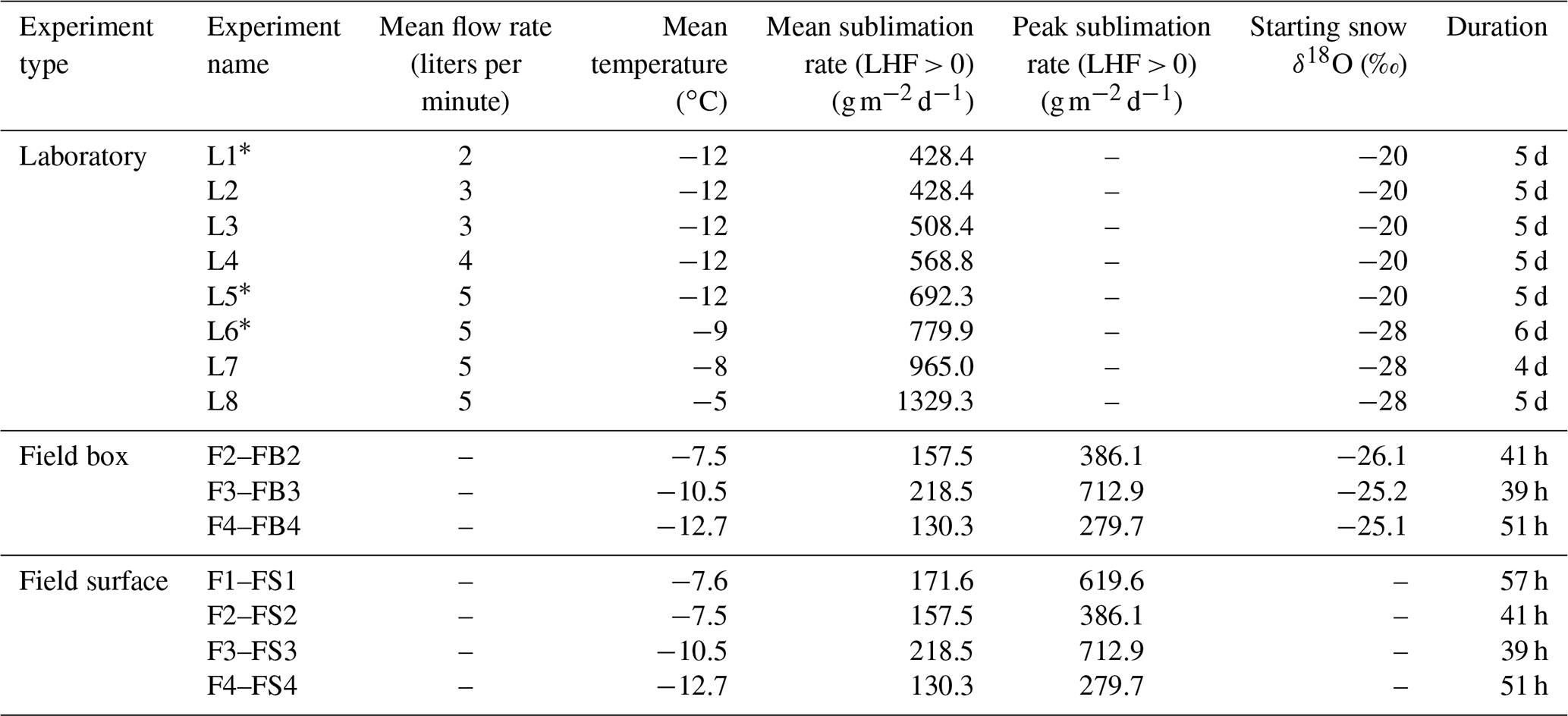
* Stars denote the subset of laboratory experiments selected for further discussion.
In this study, we investigated how the isotope signal of surface snow is altered over multiple days via post-depositional exchange between the snow and the near-surface atmospheric water vapor. We utilized multiple types of experiments including both controlled laboratory experiments and in situ field observations. First, we performed a simple laboratory experiment to observe the effects of sublimation under dry air in a controlled environment. Next, we performed two field experiments in northeast Greenland to (1) analyze the change of snow of known isotopic composition under characteristic polar conditions and (2) document the isotope signal evolution of undisturbed snow as it naturally exists at the ice sheet surface. For all experiments, continuous atmospheric vapor measurements were made above the snow surface to complement the snow sampling and allow us to observe ongoing snow–vapor isotope exchange. Thus, these laboratory and field experiments are the first to measure both δ18O and δD at fine vertical and temporal resolution for multiple depths across several multi-day experimental periods under differing environmental conditions, with simultaneous continuous measurements of atmospheric vapor δ18O and δD. In the case of the laboratory experiments presented, the vapor isotopic composition can directly be interpreted as the isotopic composition of the flux, since the experimental set-up fulfills the closure assumption and therefore allows a direct comparison of flux and snow isotopic composition. With these data we demonstrate the importance of post-depositional processes on the snow surface water isotope signal, and we provide better constraints on transfer functions between the atmospheric conditions including water vapor isotopic composition and the climate signal recorded in the surface snow, with implications for interpretation of ice core records.
We investigated through a combination of laboratory and field experiments (Table 1) the influence of phase changes (i.e., sublimation and vapor deposition) on the snow surface isotopic composition. Laboratory experiments were run in a controlled environment, which allowed us to isolate the effects of idealized sublimation conditions. The sublimation rate was varied between different experiment runs through adjusting temperature and the flow rate of dry air. Complementary field experiments provided greater insight as to how laboratory findings are consistent with field observations occurring at the surface of the ice sheet. The field experiments were run under close-to-ideal conditions, which limited the duration of the experiments to intervals of time with clear-sky conditions. In return, the sampling resolution was increased for the field experiments.
Throughout this work, water isotope measurements are reported in standard delta notation given in per mil (‰) (Craig, 1961):
where i refers to δD or δ18O, and R is the ratio of heavy to light isotopes, such that and , where 2H is referred to as D. Samples were referenced to Vienna Standard Mean Ocean Water (VSMOW).
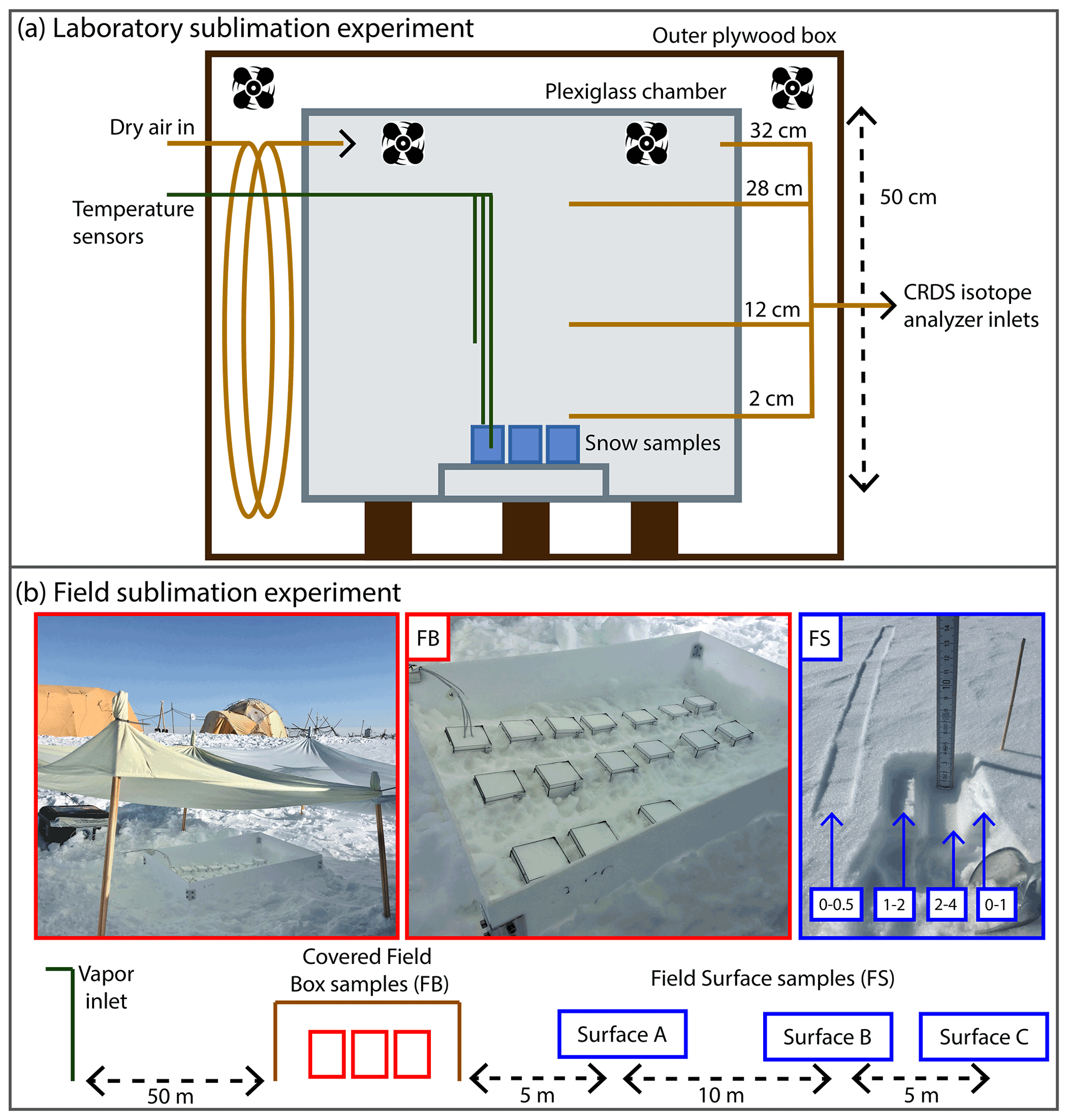
Figure 1(a) Diagram of laboratory experiment setup. A plexiglass chamber was placed within an outer plywood box in a freezer, and dry air regulated by a mass flow controller was pumped into the inner box above four to six homogeneous snow samples, placed on a small shelf to allow airflow. Fans inside the box maintained air circulation. Three temperature sensors were placed at different heights, and continuous CRDS measurements of the vapor were made at four inlet heights (2, 12, 28, 32 cm above the snow surface). (b) Schematic diagram of the field sampling setup at EastGRIP. From left to right: atmospheric vapor at 10 cm above the snow surface was continuously measured by a CRDS. Homogenous box samples (FB; red) were partially buried and covered, and temperature sensors were placed in the atmosphere, snow surface, and below the surface. Three surface sampling locations (FS A, B, C; blue) were spaced 5–10 m apart, with samples taken at every time interval at each location. A photo example of one sample is shown, in which the left-most sample is the 0–0.5 cm sample, while the intervals for 0–1, 1–2, and 2–4 cm can be seen in the small pit.
2.1 Laboratory experimental methods (L experiments)
For the laboratory experiments (L1–L8), dry air was circulated over boxes containing isotopically homogeneous snow samples that were kept at fixed temperatures (Fig. 1a). An experimental chamber was designed that consisted of an inner plexiglass box, which sat inside an outer plywood box (2.7 cm thick) used for temperature regulation. The entire setup was placed in a large freezer, with the inner temperature moderated by a PID-controlled (Omega CN7800; 50 W) cable heater wrapped around the inside of the plywood box. Dry air was produced with a generator (Puregas CDA-10) and run through Drierite desiccant, resulting in humidity <100 ppm (i.e., <5 % RH). The amount of dry air circulated in the box was regulated by a HORIBA SEC-4400 mass flow controller, and two continuously running computer fans at the top of the chamber maintained mixed air. In order to maintain positive pressure in the box, flow rates less than 2 L min−1 could not be used. Four to six small plastic boxes ( cm) were filled with snow that was well-mixed and sifted so that the snow grain size (1–2 mm) and isotope value were homogenous, and the initial mass of each sample was measured. The samples were placed at the bottom of the inner box, on a shelf with underlying airflow to prevent a temperature gradient within the samples. Every 24 h, one sample was removed, and the mass of that sample was measured. The boxes could be opened on one side, and a metal spatula was used to collect snow samples with 5 mm resolution to obtain a vertical isotope profile. Snow samples were transferred to 20 mL HDPE scintillation vials for storage and kept frozen until analysis, at which time they were melted and immediately transferred to 2 mL vials. Liquid samples were then analyzed using a Picarro L2130-i cavity ring-down spectrometer (CRDS), in conjunction with a CTC Analytics HTC PAL autosampler injection system and Picarro V1102-i vaporization module. Each sample was measured with six injections, and the reported value is based on the average of the last three injections to remove memory effects (Schauer et al., 2016). Every analysis run of 40 samples also included three known water isotope standards bracketing the sample isotope values for calibration (e.g., as done in Jones et al., 2017b). The resulting discrete measurements have uncertainties of 0.1 ‰ δ18O and 1 ‰ δD.
For the duration of all experiments, several additional parameters were monitored. A Picarro L2130-i CRDS was continuously measuring (∼1 Hz) vapor (humidity, δ18O, δD) from four heights above the snow surface (2, 12, 28, 36 cm), cycling between each level every hour. The second-order parameter d-excess (d-excess ) was also calculated from those measurements. Three Pico Technologies PT-104 data logger temperature sensors were placed in the box to record continuously: one 10 cm above the snow surface, one on the surface of the snow, and one ∼4 cm below the snow surface.
Two sets of experiments were conducted with varying sublimation rates controlled by adjusting temperature and dry air flow rate (Table 1). For five experiment runs, the temperature was held steady at −12 ∘C while the dry air flow rate was changed between a constant flow rate of 2, 3, 4, and 5 L min−1 (L1–L5, respectively). These experiments used snow from Boulder, Colorado, with a starting value of approximately −20 ‰ δ18O, and they were carried out at the Institute of Arctic and Alpine Research at the University of Colorado Boulder. Three additional experiment runs had the temperature of the inner box held constant at −9, −8, or −5 ∘C (L6–L8, respectively), and the flow rate of dry air above the snow samples was held steady at 5 L min−1. These experiments used snow from the East Greenland Ice Core Project field site with a starting δ18O value of approximately −28 ‰ and were completed at the section for Physics of Ice, Climate and Earth at the University of Copenhagen. In total, eight experiments were completed.
2.2 Field experimental methods (F experiments)
Field experiments were conducted at the East Greenland Ice Core Project (EastGRIP) field camp in July 2019. EastGRIP is located at 75.6268∘ N, 35.9915∘ W in the accumulation zone of the Greenland Ice Sheet. In July 2019, the meteorological conditions at the site were characterized by low temperatures (mean −9.0 ∘C, measured at 2 m above the snow surface) and high relative humidities (mean 91 % RH with respect to ice), leading to an average specific humidity of 2.3 g kg−1. Positive temperatures (>0 ∘C) were very rare, and we observed a positive change in snow height of about 2 cm during July.
The goal of in situ field experiments was to characterize interactions between the snow surface and near-surface atmospheric vapor on short timescales and to monitor the evolution of the isotopic signal in the snow. To do so, we selected four 2–3 d experimental periods (field experiments, F1–F4) during which changes in water isotopes in the snow surface and atmospheric vapor were measured simultaneously through three sample types (Fig. 1b): (1) discrete box samples (field box, FB2–FB4), (2) discrete surface samples (field surface, FS1–FS4), and (3) continuous vapor measurements at 10 cm above the snow surface. Each experiment was conducted during a period of good weather, such that precipitation or windblown snow would not bias results. This required air temperatures below freezing, sustained wind speeds below 5–6 m s−1, and no precipitation.
2.2.1 Discrete box samples (FB experiments)
At the beginning of each period, 14–16 boxes ( cm) were filled with well-mixed surface snow. Sampling boxes were partially buried in the snow surface, with the top of the sample box 1–2 cm above the surrounding snow surface to minimize any risk of contamination from windblown snow. Samples were also protected from direct overhead sunlight using a light-colored thin cloth covering. Although this deviates from natural conditions in which the snow surface is exposed and not covered, this modification was necessary to prevent solar heating of the sample boxes which may have led to melt of the snow samples. A Pico Technologies PT-104 data logger was used to measure temperature during the experimental period, with four sensors placed in an additional snow-filled box. The logger continuously recorded temperatures of the ambient air, snow surface, 3 cm below surface, and 6 cm below surface.
One box was collected every 3 h; each box was equipped with one removable side so that a vertical profile of the snow was accessible. Snow samples were taken at intervals 0–0.5, 0.5–1, 1–1.5, 1.5–2.5, and 2.5–4.5 cm from the surface using a spatula. The snow samples were transferred to a 20 mL HDPE scintillation vial for storage. Discrete samples are referred to as field box (FB) samples, with each experiment designated FB2, FB3, and FB4 (Table 1).
2.2.2 Discrete surface samples (FS experiments)
In addition to the isolated boxes, every 3 h we collected samples from a clean, undisturbed surface snow area at the same time as the boxes were sampled. Because wind effects can lead to variability in snow surface density and isotopic value, surface samples were collected from three locations, designated sites A, B, and C. The distance from A to B was 10 m and from B to C was 5 m (Fig. A1). At each surface location, samples were collected from 0–0.5, 0–1, 1–2, and 2–4 cm below the surface (Fig. 1b). The snow samples were transferred to a 20 mL HDPE scintillation vial for storage. Discrete surface samples are referred to as field surface (FS) samples, with each experiment designated FS1, FS2, FS3, and FS4 (Table 1).
All snow samples (both field box (FB) and field surface (FS)) were kept frozen after collection and were measured at the Stable Isotope Lab at the University of Colorado Boulder. Samples were analyzed using a Picarro L2130-i, in conjunction with a CTC Analytics HTC PAL autosampler injection system and Picarro V1102-i vaporization module. The same measurement protocol was used as described in Sect. 2.1.
2.2.3 Continuous vapor measurements
Continuous atmospheric water vapor isotope measurements were made at 10 cm above the snow surface, ∼50 m away from the FS sampling site so as not to be contaminated by snow sampling activity. The measurements were made with a Picarro L2130-i CRDS, which was kept in a temperature-controlled tent and measured humidity, δ18O, and δD. Using a diaphragm pump (KNF model DC-B 12V UNMP850), air was pumped through a ∼12 m long heated copper tube to the analyzer (similar to the setup described in Madsen et al., 2019).
Four types of calibrations were performed on the water vapor isotope measurements of the CRDS, similar to the calibration protocol described in Steen-Larsen et al. (2013): (1) humidity calibration, (2) humidity-isotope response calibration, (3) VSMOW-VSLAP scale calibration, and (4) drift calibration. All calibrations are applied to water vapor isotope measurements in both laboratory and field experiments. Details of the calibration setup specific to laboratory and field experiments are described in Appendix B.
Latent heat flux (LHF) was also continuously measured during the field campaign using a Campbell Scientific IRGASON eddy-covariance (EC) system. The two-in-one EC system measured humidity and three-dimensional wind at a sampling frequency of 20 Hz in the same sample volume at 2.15 m above the snow surface. LHF values were computed for 30 min intervals using Campbell Scientific's software EasyFlux™ adjusted for sublimation conditions and accounting for wind rotation and frequency corrections. Latent heat flux is related to sublimation: LHF = sublimation rate⋅λ, where λ is the latent heat of sublimation at 0 ∘C, 2834 kJ kg−1; a positive LHF indicates sublimation, and negative LHF indicates vapor deposition.
3.1 Laboratory experiments
3.1.1 Sublimation rate
The mean sublimation rate for each laboratory experiment is calculated based on mass loss with time and surface area, reported in Table 1. Sublimation rate does not significantly change with time and is shown for each experiment in Fig. A8. The mass of each box was measured at the onset of the experiment and immediately before each sampling. Since we only push dry air into the chamber, the experiment relates only to sublimation processes. We find that the LHF associated with sublimation varies from approximately 15 W m−2 (Experiment L1 at 2 L min−1 and −12 ∘C) to 44 W m−2 (Experiment L8 at 5 L min−1 and −3 ∘C).
Latent heat flux values in laboratory experiments are comparable to the peak daytime sublimation fluxes observed during the field campaign, albeit the average LHF during the sublimation period in the field was substantially smaller than observed during the laboratory experiments (Table 1). The mean daytime positive LHF was ∼5 W m−2, and the maximum LHF observed was ∼23 W m−2. Therefore, laboratory experiments can be considered representative of processes occurring during peak daytime conditions in the field.
3.1.2 Snow measurements
Eight laboratory experiments (L1–L8) were completed, with temperature, dry air flow rate, and sublimation rate documented in Table 1. In all experiments, the surface snow experiences substantial isotopic changes, with δ18O increasing by up to 8 ‰ and d-excess decreasing by over 25 ‰. δ18O and d-excess signals for all experiments are shown in Fig. A10, with a subset of experiments shown in Fig. 2. Changes in the isotope signal are observed to propagate several centimeters into the snowpack due to diffusion over 4–6 d, driven by the induced sublimate-related isotope change at the surface. The rate of change is calculated for the mean isotope value for each day of sampling, ranging from 0.25–0.70 ‰ d−1 for δ18O and 0.66–2.64 ‰ d−1 for d-excess (Fig. A11a and b). There is a strong relationship between mass loss and isotope values, with an average R2=0.90 for daily mean box δ18O vs. mass loss for experiments L1–L8. The relationship between sublimation rate and δ18O rate of change has R2=0.13, and sublimation rate vs. d-excess rate of change has R2=0.54 (Fig. A11c).
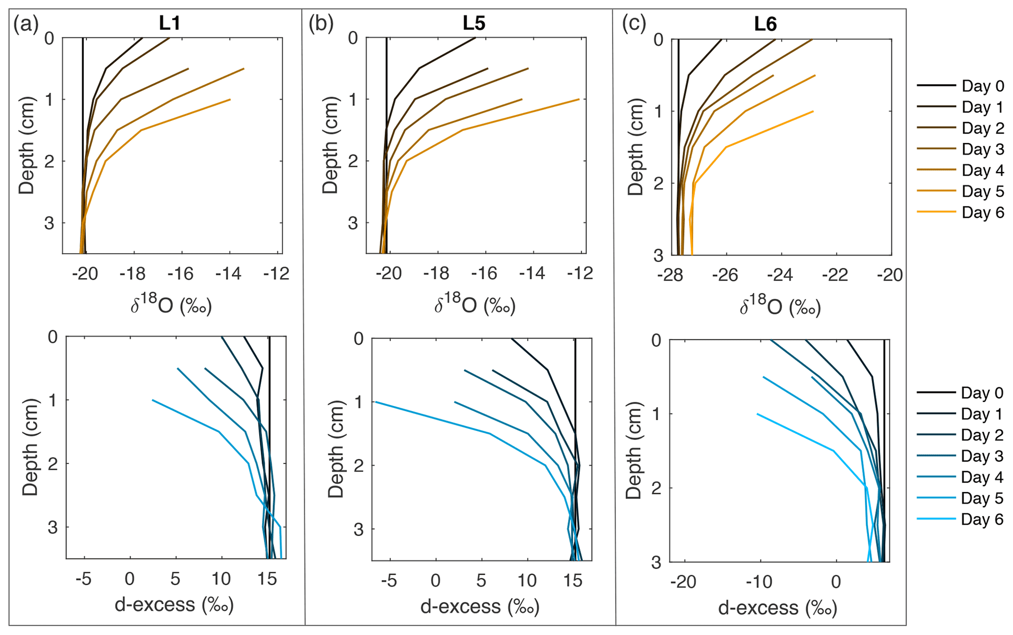
Figure 2Snow δ18O (top) and d-excess (bottom) vertical profiles from three of the laboratory experiments: (a) L1 (−12 ∘C, 2 L min−1), (b) L5 (−12 ∘C, 5 L min−1), and (c) L6 (−9 ∘C, 5 L min−1). Day 0 (black) represents the initial homogeneous snow sample, with colors progressively moving towards orange (δ18O) and blue (d-excess) with each day of sampling. As each experiment progresses from Day 0 to Day 6, sublimation drives an increase in δ18O and decrease in d-excess, with the greatest change at the snow surface. Similar figures for all laboratory experiments (L1–L8) can be found in Fig. A10.

Figure 3(a) d-excess vs. δ18O is shown for the vertical snow profile at each day of sampling in Experiment L5, with a linear regression calculated for each day. This gives a slope of d-excess vs. δ18O, which evolves with time. (b) The slope of d-excess vs. δ18O with time is shown for each experiment L1–L8, demonstrating an inverse relationship between sublimation rate and slope of d-excess vs. δ18O. Error bars indicate 95 % confidence intervals for each slope.
Because δ18O reflects equilibrium fractionation and d-excess is influenced by kinetic fractionation, a comparison of these variables provides insight into the extent of fractionation effects occurring during sublimation. The slope of d-excess vs. δ18O is calculated for samples within each box (Fig. 3a), and the slope with time over the duration of each experiment is shown in Fig. 3b. The slope ranges from −0.91 ‰ to −3.57 ‰ d-excess/‰ δ18O and decreases over the course of all experiments. In general, there is a decrease in slope associated with an increase in sublimation rate, as indicated by the color scale reflecting sublimation rate in Fig. 3b and as shown in Fig. A9.
3.1.3 Vapor measurements
During all laboratory experiments, a Picarro L2130-i CRDS was used to continuously measure vapor in the chamber at 2, 12, 28, and 36 cm, cycling through each height for 1 h measurement periods. We exclude the first 20 min of each measurement period to remove memory effects from valve changes. Figure 4 shows an example of temperature and vapor data for experiment L5, including the 28 and 32 cm levels, which represent sublimated vapor which is more well-mixed than that immediately above the snow surface. Dry air pumped into the top of the box is mixed using a set of fans creating turbulence above the snow surface. The vertical differences in humidity and isotopic composition of the air in the box (i.e., differences between 28 and 32 cm as seen in Fig. 4) likely indicate that the ventilation is not strong enough to maintain a fully homogeneous air mass in the box, allowing for a slight vertical gradient.
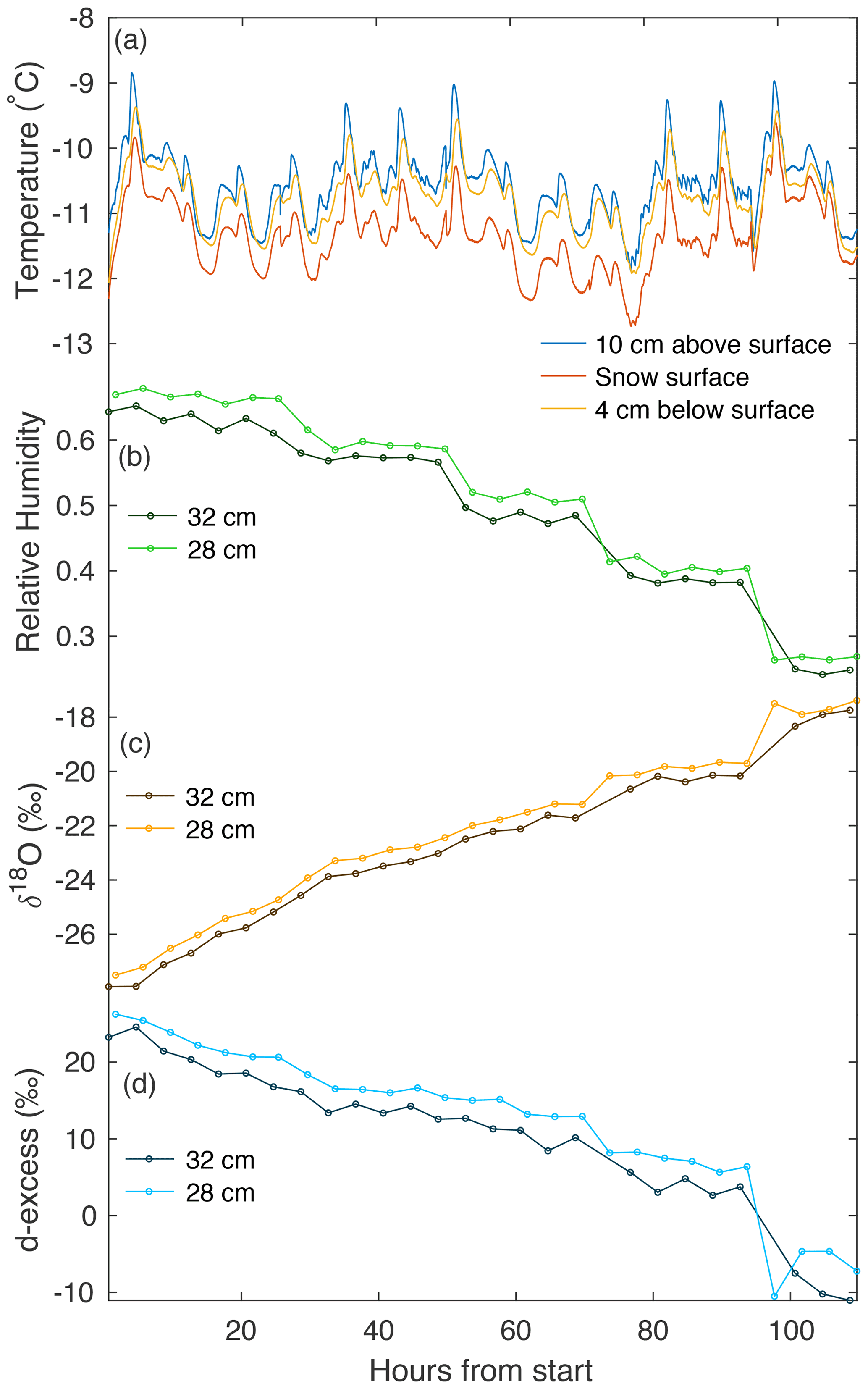
Figure 4An example of continuous temperature and vapor measurements from experiment L5. (a) Three temperature sensors continuously measure at different heights with respect to the snow surface (10 cm above, on the surface, and ∼4 cm below the surface). A CRDS measured (b) humidity, (c) δ18O, and (d) d-excess in vapor, continuously cycling at four heights. Panels (b–d) show vapor measurements at 28 and 32 cm above the snow surface. We document the average of each measurement period, with the first 20 min excluded to remove memory effects.
Over the course of each 4–6 d experimental period, we observe several trends in vapor measurements consistent across all laboratory experiments. Humidity decreases with time, due to a reduction in the sublimating surface area each time a snow sample box is removed. Vapor δ18O increases with time, consistent with the increase in δ18O observed in the snow surface. Similarly, d-excess decreases with time in both vapor measurements and the snow surface.
3.2 Field experiments
Four experiments (F1, F2, F3, F4) were carried out during the 2019 EastGRIP field season, with surface samples (FS1, FS2, FS3, FS4) collected for all experiments and box samples (FB2, FB3, FB4) collected for three experiments. Each of the four experiments lasted 40–60 h and is supported by continuous measurements of near-surface (10 cm) atmospheric vapor (δ18O, δD, d-excess, humidity), temperature (snow and atmosphere), and LHF. Within each experiment, surface snow and box samples are collected every 3 h. The duration and average environmental conditions of each experiment are reported in Table 1. A compilation of results for measurements of FS, FB, and atmospheric vapor is shown in Fig. 5 and discussed in the next section. All FS and FB samples are shown in Figs. A12 and A13, respectively, with additional vapor measurements shown in Fig. A14.

Figure 5A compilation of data from the 2019 field season shows atmospheric measurements and surface snow samples; from top: latent heat flux (red, positive values; blue, negative values; dashed gray line at 0), δ18O (green) of atmospheric vapor (2 min average) measured at 10 cm, δ18O of the top sample (0–0.5 cm) of the FB box sample (pink dashed), and δ18O of FS snow surface samples. Each snow surface sampling interval shown represents the average of three surface sampling locations (A, B, C) for four different depth intervals: 0–0.5 cm (black), 0–1 cm (red), 1–2 cm (orange), and 2–4 cm (yellow). δ18O of FS samples tends to reflect δ18O in atmospheric vapor, with the relationship strongest in the upper surface samples (Table 3). Additional data including temperature and vapor humidity are shown in Fig. A14.
3.2.1 Variability in δ18O and d-excess of surface snow
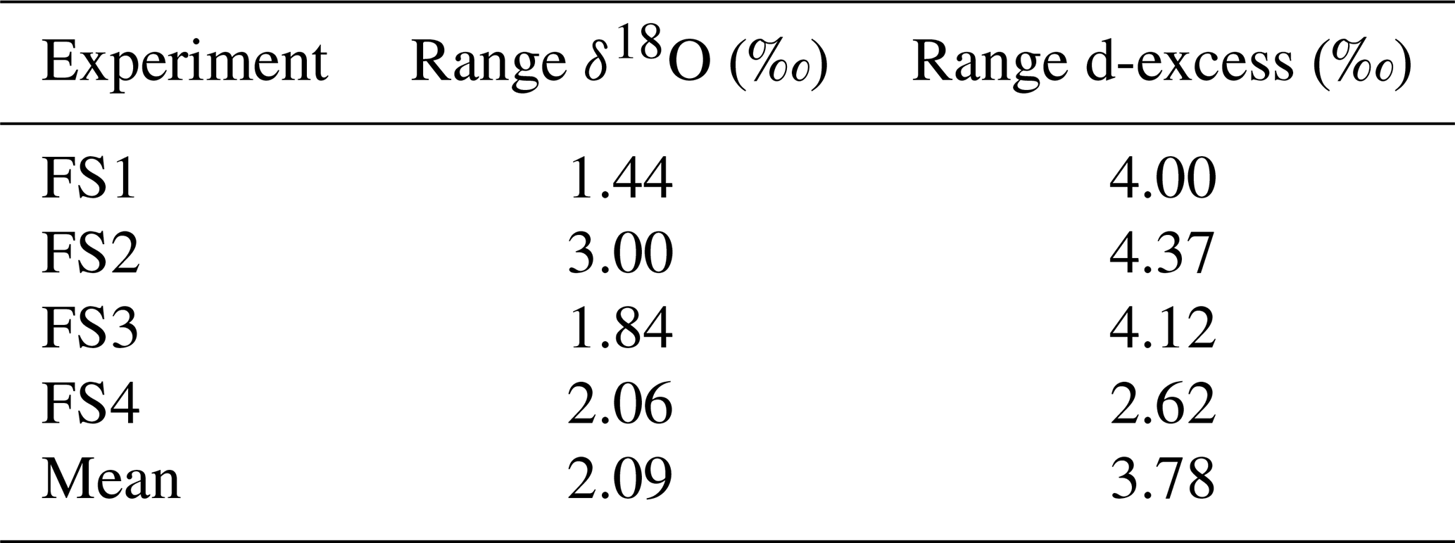
In order to account for horizontal and vertical spatial variability as a result of redistribution of snow in sastrugi and snow dunes, we averaged isotope values across the three surface locations (A, B, C) for each time of sampling and for each depth interval (i.e., one averaged value each for 0–0.5, 0–1, 1–2, and 2–4 cm at every time sampled). In the following figures and tables we focus on the location-averaged values for each sampling time and depth, referred to as FS1, FS2, FS3, and FS4 for each FS surface experiment. Isotope values for all surface locations (A, B, C) are shown together with the averages in Fig. A12. Location-averaged surface snow measurements at all depths across FS1, FS2, FS3, and FS4 range from approximately −30.3 ‰ to −20.7 ‰ δ18O and 4.6 ‰ to 14.3 ‰ d-excess. In all experiments, we consistently observe changes in surface snow isotopic composition on an hourly timescale (Fig. 5). The maximum change in average δ18O of the top surface sample (0–0.5 cm) during a single experiment occurred during FS2, which experienced an enrichment of 3 ‰ δ18O and decrease of 4.37 ‰ in d-excess. This evolution is substantially smaller than the isotopic change observed in vapor measurements, which has ranges of 5 ‰–12 ‰ δ18O over individual experiment periods and ranges for d-excess of 15 ‰–24 ‰. The maximum change in δ18O and d-excess observed within the top surface sample (0.0–5 cm) during each experiment is reported in Table 2.
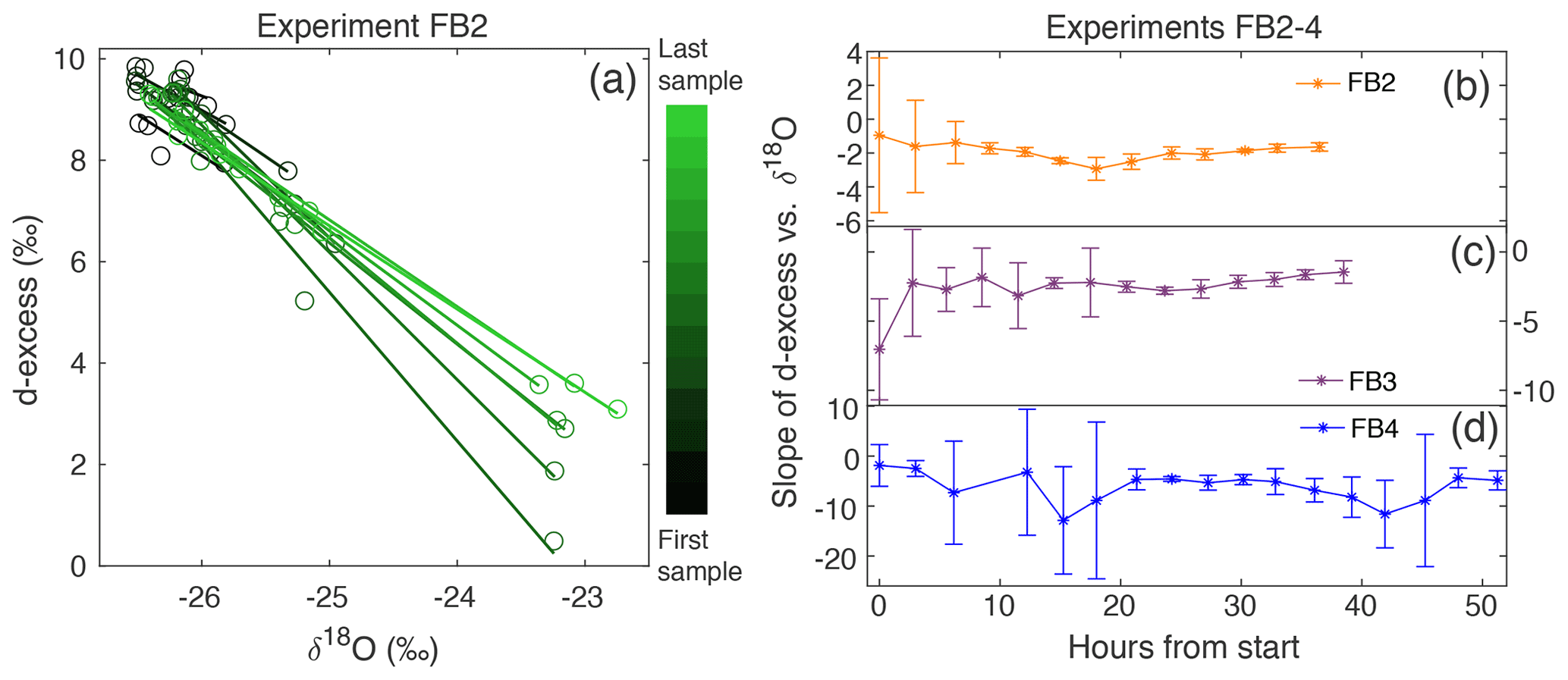
Figure 6(a) d-excess vs. δ18O is shown for the vertical snow profile at each time of sampling in Experiment FB2, with a linear regression calculated for each day. This gives a slope of d-excess vs. δ18O, which evolves with time. The sampling time is indicated by the color scale from black (first sample taken) to light green (last sample taken). The slope of d-excess vs. δ18O with time is shown for experiments (b) FB2, (c) FB3, and (d) FB4. Error bars indicate the 95 % confidence interval for each slope.
Table 2The maximum range of isotope measurements is shown for the mean value of the top (0–0.5 cm) sample for all FS experiments.
3.2.2 Relationship between vapor and surface snow
Over the course of all experiments, the minimum atmospheric vapor δ18O value observed is −50 ‰, while the maximum observed value is −33 ‰ (a range of 17 ‰). Within each 40–60 h long experiment, the minimum range of variability observed is about 5 ‰ (F4), and the maximum is about 12 ‰ (F3). Vapor δ18O co-varies with humidity and temperature (Fig. A14), with the lowest δ18O measurements observed during cold, dry conditions. A clear diurnal cycle is observed in vapor measurements for experiments F3 and F4, while experiments F1 and F2 are more variable. The change in atmospheric δ18O associated with the diurnal cycle is much smaller than that observed during synoptic weather changes, similar to the pattern previously observed at the northwest Greenland site NEEM (Steen-Larsen et al., 2014). For example, we observe a strong diurnal cycle in F4 and the first half of F3, both of which have an amplitude of approximately 5 ‰–6 ‰ δ18O; the change between experiments with different synoptic-scale atmospheric conditions is much greater (i.e., a 17 ‰ δ18O range is observed between the maximum value during F2 and the minimum value during F4).
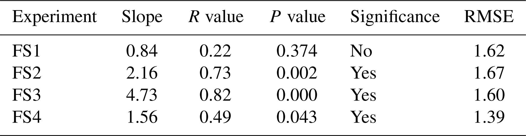
Over clear-sky experimental periods with no precipitation, we observe the δ18O value of surface snow increasing and decreasing on an hourly timescale, corresponding to changes in vapor δ18O (Fig. 5). To compare the evolution of the isotope signal in vapor and snow measurements, the vapor δ18O is downsampled to 3 h resolution to match snow sampling resolution. A statistically significant (p≤0.05) relationship is observed between δ18O of 0–0.5 cm snow surface samples and atmospheric vapor measurements for experiments FS2, FS3, and FS4, but not FS1 (Fig. A15, Table 3). The lack of a significant correlation in FS1 may be a result of some synoptic-scale weather difference, as it is the only experiment period in which there is a sustained decrease in vapor δ18O, and a diurnal cycle in temperature, LHF, and vapor δ18O is least distinguishable.
Table 3The R value, P value, and root-mean-square error (RMSE) are documented for the relationship between the top (0–0.5 cm) FS sample δ18O and interpolated vapor δ18O. Significance is determined by p≤0.05. δ18O of vapor vs. surface samples is shown in Fig. A15.
In the laboratory experiments, the snow was sublimating under dry air, resulting in a higher LHF than was observed in a typical field setting. For this reason, laboratory experiments are considered an extreme example of natural processes and can be used to identify and understand the physical processes associated with sublimation which would occur on a slower timescale in nature. Laboratory results show a strong signal of enrichment in the snow surface δ18O, as light isotopes preferentially sublimate from the surface due to fractionation. In addition we observe a strong decrease in the snow surface d-excess. Decreasing d-excess driven by kinetic fractionation is also observed when a body of water evaporates into a sub-saturated atmosphere (Benson and White, 1994; Merlivat and Jouzel, 1979). As a similar effect is observed during sublimation in laboratory experiments, we draw the analogy that this is due to kinetic fractionation. This aligns with previous experimental and modeling studies (Ritter et al., 2016; Ebner et al., 2017) and confirms our hypothesis that the upper several centimeters of the snow surface are rapidly (i.e., on a sub-daily timescale) influenced by equilibrium and kinetic fractionation during sublimation. This contradicts the traditional theory of sublimation, which states that sublimation occurs layer by layer and does not alter the snow isotopic composition, on which ice core paleoclimate water isotope research has been resting (Dansgaard et al., 1973).
In order to interpret these results in the context of natural processes, we consider the results of the field experiments. Previous studies have shown that significant isotopic changes of surface snow are observed (using daily sampling resolution) over periods of time without precipitation, and this is associated with snow metamorphism (Steen-Larsen et al., 2014; Casado et al., 2018). We expand on these findings with higher-resolution field sampling, showing that snow surface δ18O and d-excess change on an hourly basis, which was hypothesized by Madsen et al. (2019); this demonstrates that similar processes to the lab experiments are occurring in a natural environment, albeit less extreme.

Figure 7Comparison of latent heat flux (LHF) and 0–0.5 cm samples for mean FS surface samples and FB box samples for (a) F2, (b) F3, and (c) F4. Positive LHF values are indicated in red, and negative LHF values are marked blue with associated shading in all subplots (LHF, δ18O, and d-excess). FS surface snow 0–0.5 cm values are shown in brown (δ18O) and dark blue (d-excess), with each location (A, B, C) designated by dashed lines and the mean of all locations as the bold solid line. FB box snow 0–0.5 cm values are shown in light orange (δ18O) and light blue (d-excess) bold lines.
To interpret the driving factors in snow isotope changes, we consider differences between the FB box and FS surface samples. The FB samples were covered to shield from direct sunlight and windblown snow and therefore were less likely to experience vapor deposition or frost. Figure 7 shows a comparison of the top 0–0.5 cm sample for all FB and FS experiments with LHF. Over the course of the field experiments, we observe several 6–12 h periods of increasing δ18O in 0–0.5 cm FB and FS samples, primarily during periods of positive LHF and decreasing d-excess; this is indicative of sublimation as suggested by laboratory experiments and model results. We also observe several 6–12 h periods in which the FS δ18O decreases, despite experiments taking place during time periods with no precipitation and minimal wind-drifted snow. Periods of decreasing FS δ18O occur primarily during nighttime hours with negative or low LHF measurements (Fig. 7; negative LHF indicated by shading) and increasing d-excess. There is no significant decrease in δ18O in FB2 and FB3 associated with these periods, while there is a simultaneous decrease in δ18O in FB4 and FS4. Additionally, the 0–0.5 cm d-excess decreases substantially in all FB experiments, similar to the signal that was observed due to kinetic fractionation during sublimation in laboratory experiments. In general, the box samples experience less decrease in δ18O than associated FS samples due to minimized vapor deposition during periods of negative LHF and greater total decrease in d-excess due to increased total sublimation across the entire experimental period. This demonstrates that vapor deposition of preferentially isotopically heavy water molecules in the form of frost significantly contributes to the surface snow signal on a rapid timescale (Casado et al., 2018).
There are still several factors in the field experiments which could complicate interpretation of the results. While it is clear in the laboratory experiments that any changes in the snow composition are a direct result of sublimation, we cannot isolate individual processes occurring in field experiments. For example, atmospheric vapor δ18O measurements often vary in phase with LHF, but during some periods (most notably the latter half of F1 and F3) vapor δ18O deviates from the LHF trend. At this stage it is unclear whether LHF, vapor δ18O, or another factor is influencing the snow surface, or whether the snow surface composition is driving vapor δ18O. Additionally, the isotopic composition of deeper snow layers could influence the surface snow due to diffusion. We note a general trend observed in Experiments FS1, FS2, and FS3 in which the deepest surface sample (2–4 cm) has the lowest values for both δ18O and d-excess. However, throughout the duration of FS4, the upper samples (0–0.5, 0–1, and 1–2 cm) have a lower δ18O value than the 2–4 cm sample, likely due to a precipitation event preceding FS4 which may have deposited surface snow with anomalously low δ18O. If there are significant differences between the composition of adjacent snow layers, the surface snow could be influenced by a combination of interstitial diffusion and atmospheric driving forces (i.e., LHF and vapor δ18O). This may also explain some isotope inter-experiment differences between FB and FS results, as FB samples are homogeneous and FS samples have vertical variability in snow isotopic composition.
A key finding from field experiments is that both sublimation and vapor deposition influence the surface snow on an hourly timescale; this is supported by laboratory experiments, demonstrating that sublimation has the ability to influence the mean surface snow isotopic composition in the top 1–2 cm of the snowpack during precipitation-free periods. These changes are occurring faster than the average recurrence of precipitation events and could produce substantial changes in the mean isotopic composition of the upper several centimeters of the snowpack over a long precipitation-free period. This suggests that effects from sublimation and vapor deposition may be superimposed on the precipitation signal, resulting in a snowpack record indicative of multiple parameters including atmospheric conditions, water vapor isotopic composition, condensation temperature (i.e., δ18O), and precipitation source region conditions (i.e., d-excess). The extent to which this occurs is dependent on the accumulation rate at the ice core site, as these processes primarily influence the top few centimeters of the snow column. A site such as SE-Dome (southeast Greenland), which receives 102 cm yr−1 of ice equivalent precipitation (Furukawa et al., 2017) (i.e., several meters of snowfall), will be less affected than a drier location with significantly less annual accumulation, such as Antarctic sites like WAIS Divide (24 cm annual accumulation) (Fudge et al., 2016) or South Pole (7.4 cm annual accumulation) (Mosley-Thompson et al., 1999).
To assess the relevance of our results on longer timescales, we make use of a simple mass balance calculation and an observed mean LHF in July of 3.1 W m−2, indicating a net removal of snow from the surface due to sublimation. By assuming equilibrium fractionation during sublimation (Wahl et al., 2021), we can calculate the isotopic composition of the humidity flux and the associated removal of isotopologues. When considering reasonable values of a 5 cm layer of snow, a snow density of 300 kg m−3, an initial isotopic composition of −20 ‰ δ18O, and a surface temperature of −9 ∘C for the month of July, the snow would be enriched by ∼4 ‰ δ18O due to the net humidity flux, which is substantial. For comparison, the seasonal amplitude (i.e., summer peak to winter trough) at the Renland Ice Cap, for example, is about 8 ‰ in δ18O (Hughes et al., 2020). We acknowledge that this is a highly simplified mass balance calculation without taking into account the vapor isotopic composition or precipitation inputs. However, since vapor exchange is a continuous process, it will continuously affect the layer of snow that is in contact with the atmosphere and will therefore imprint on the snow isotopic composition with a general net daily sublimation signal during months with a net sublimation flux.
Which months show a net sublimation flux is dependent on the geographical location and general climatology of the area. Especially in the context of paleoclimatological interpretation of ice cores, this cannot be assumed to be constant in time. If the vapor–snow exchange imprints on the seasonal snow isotopic composition as indicated in the result of the mass balance calculation, one would need to take changes in sublimation seasonality into account when making assumptions about vapor-exchange effects on paleo timescales, as has been previously demonstrated for precipitation seasonality (Werner et al., 2000).
On shorter timescales in our laboratory experiments we observe changes of up to 8 ‰ δ18O and 20 ‰ d-excess over time periods of several days, and in FS field experiments we find an average change of 2.09 ‰ δ18O and 3.78 ‰ d-excess on very short (sub-diurnal) timescales. This observation, in combination with our mass balance calculation of 4 ‰ change in δ18O over the month of July, suggests that under typical natural conditions, changes in the surface isotope value occurring on a short timescale may have an impact on the mean seasonally recorded isotope signal. Previous studies have addressed the effect of seasonally biased accumulation rate on diffusion and the recorded δ18O isotope signal (Persson et al., 2011; Casado et al., 2020; Hughes et al., 2020) and the effect of physical modifications and snow redistribution of the snow surface on the accumulation intermittency (Zuhr et al., 2021), but the effect of sublimation-driven changes in surface snow isotopic composition between precipitation events has not been quantified previously. Whether the magnitude of the mean isotope change due to sublimation and snow–vapor exchange outweighs the effects of snow redistribution, accumulation bias, and diffusion has yet to be determined. This could be further explored through future experiments which account for additional variables or are completed at a larger scale. For example, the effect of snow specific surface area (SSA) could be determined by making simultaneous SSA and isotope measurements. Additionally, to remove the effect of wind redistribution and snow dunes on snow isotope spatial variability, a large pit could be filled with homogeneous snow for continuous sampling. In this case, the snow would have a known starting isotopic composition, similar to the FB experiments completed here but be subject to more natural conditions as in the FS experiments. Finally, as weather conditions would allow, it would be beneficial to have multiple experimental periods greater than 48 h.
In order to fully understand the implications of sublimation and vapor deposition on the ice core record, it is necessary to quantify the effects of these processes over the course of a full year. While not in the scope of this paper, this problem can first be approached through mass and isotope flux measurements throughout the summer field season (Wahl et al., 2021). Subsequent modeling of these processes throughout the annual climate cycle will provide insight as to what magnitude snow–vapor exchange influences surface snow on longer timescales (i.e., months to years), and how it may be recorded in the ice core isotope record. This could inform us to what extent changes in frequency of precipitation events, accumulation rate, and LHF could influence the isotope signal recorded in ice cores on decadal to millennial scales. Our findings suggest that these variables contribute to a combined isotope signal, in which δ18O and d-excess in ice core records likely incorporate individual precipitation events (i.e., condensation temperature and moisture source region conditions, respectively), surface redistribution (i.e., wind drift and erosion), and a post-depositional alteration signal reflecting atmospheric conditions at the ice core site. Snow isotope models such as CROCUSiso (Touzeau et al., 2018), the Community Firn Model (Stevens et al., 2020), and isotope-enabled climate models would therefore be updated through the incorporation of isotope fractionation during sublimation, snow–vapor isotope exchange, and snow metamorphosis.
In this study, we have combined controlled laboratory experiments with field measurements in an effort to constrain the effects of sublimation on surface snow isotopic composition. Experiments in a controlled laboratory setting demonstrate isotopic enrichment due to fractionation occurring during sublimation. In experimental results, δ18O increases as light isotopes preferentially sublimate due to fractionation, and d-excess decreases due to kinetic fractionation. These changes occur rapidly, substantially changing the isotopic composition of the top 2–3 cm of snow over a 4–6 d period. Field experiments included continuous measurements of atmospheric vapor and latent heat flux during periods of high-resolution surface snow sampling, during which we observed significant changes in the top 1–2 cm of snow surface isotopes on a sub-diurnal timescale. We observed periods of increasing and decreasing δ18O, indicating that both sublimation and vapor deposition influence the surface snow on an hourly basis. This supports our hypothesis that rapid change occurs in a natural setting and propagates into the snowpack, moderately altering the initial precipitation isotope signal.
Post-depositional effects have implications for the interpretation of ice core data, which traditionally is assumed to only record isotopic variability from precipitation. Our results complement previous studies demonstrating spatial and temporal variability in snow surface isotopes, further strengthening the idea that the ice core record not only integrates the climate signal of condensation temperature (i.e., δ18O and δD) and moisture source conditions (i.e., d-excess) during precipitation, but also may integrate the atmospheric conditions between precipitation events (in both δ18O and d-excess). These factors should in the future be included in isotope-enabled climate models, which may include estimates of synoptic-scale patterns across annual cycles that would influence latent heat flux, vapor composition, and the resulting influence on surface snow isotopes. This will improve future interpretations of ice core data and may be the missing link in the transfer function between climate and an uninterrupted isotope record, strengthening our interpretation of ice core water isotopes as a proxy for a continuous integrated climate record.

Figure A1(a) A photo of the FS sampling location shows the proximity between individual samples and sites. In the foreground is FS site A being sampled, with sites B and C seen in the background. The full laboratory experimental setup, with the top of the outer plywood box removed, is shown in (b), with the inside of the plexiglass chamber shown in (c).
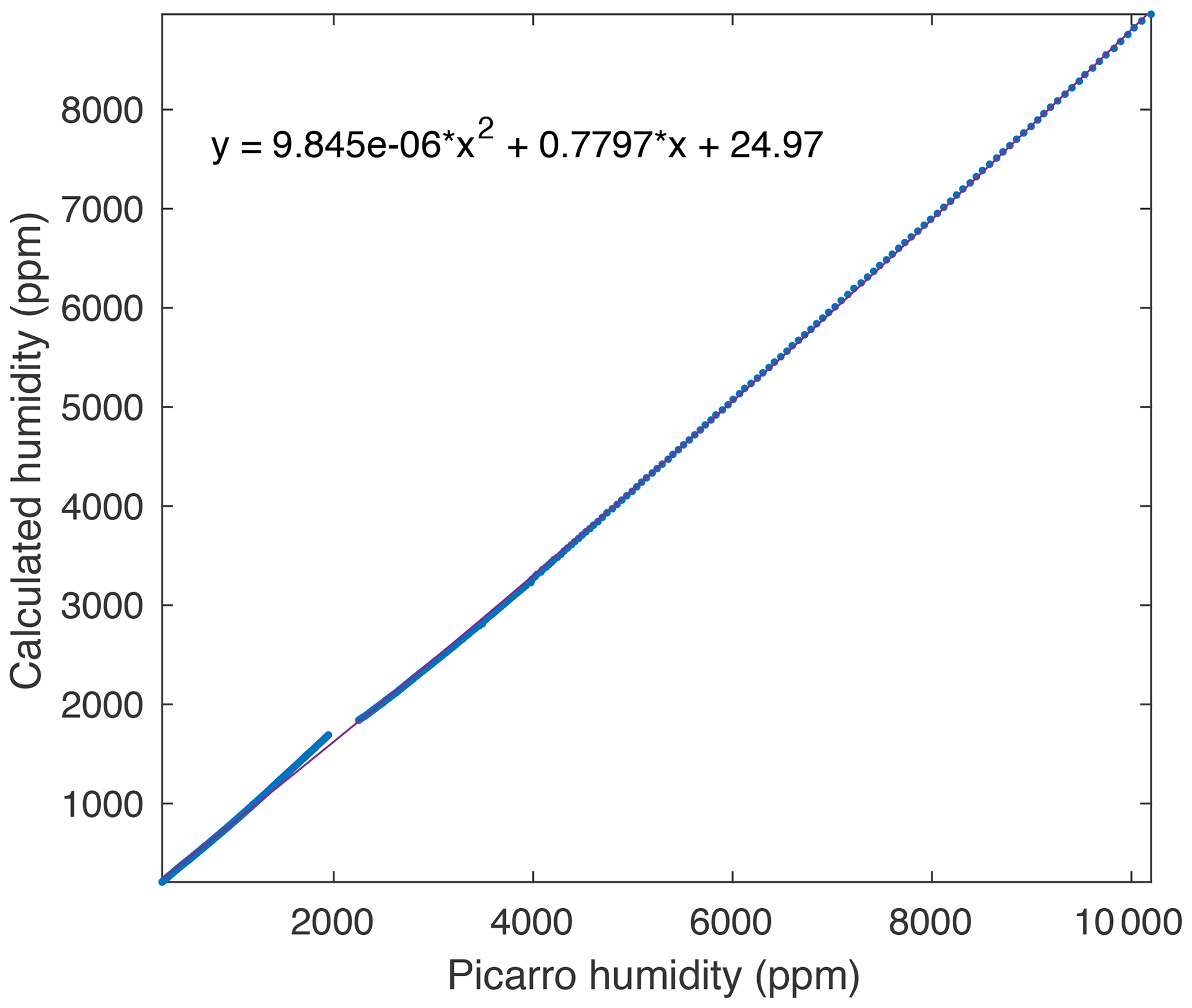
Figure A2A comparison between measured and true humidity (determined from saturation temperature) yields a quadratic response, which is used to calibrate the measured humidity.
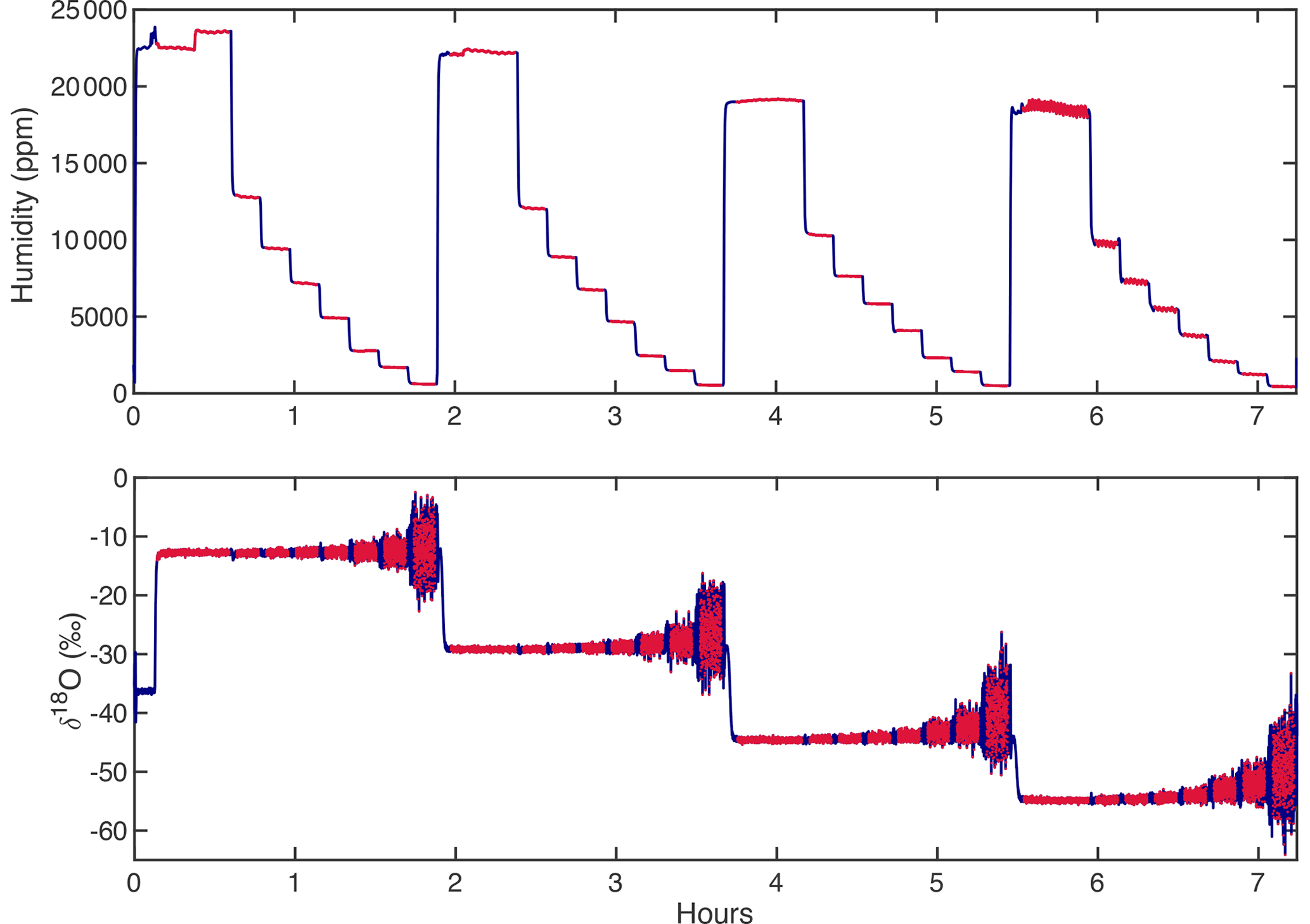
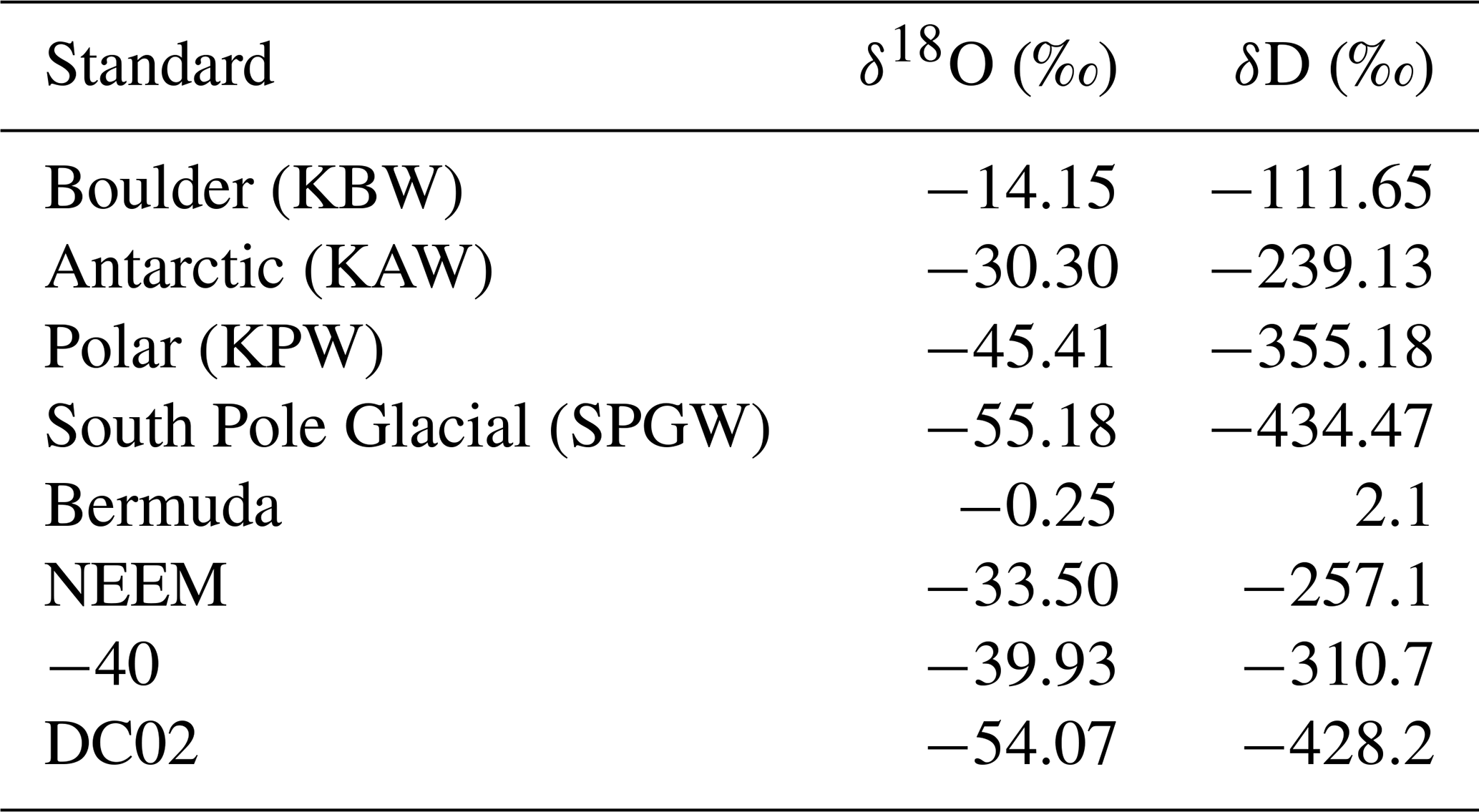
Figure A3An example of a calibration sequence shows each standard (i.e., KBW −14.15 ‰, KAW −30.30 ‰, KPW −45.41 ‰, SPGW −55.18 ‰ δ18O) measured at multiple humidity levels for 12–20 min. The full calibration sequence (blue) is trimmed (red) such that the transition periods between humidity intervals and isotopic standards are ignored, and the average value of each trimmed period is calculated.
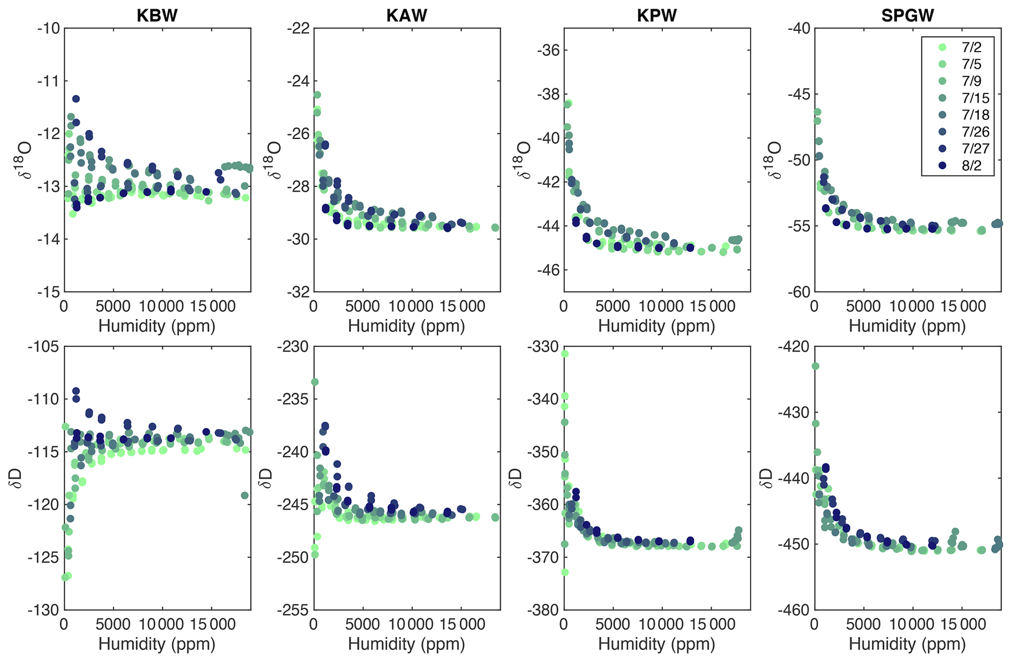
Figure A4A compilation of all calibration runs from the 2019 EastGRIP field season demonstrates slight drift in the isotopic values, particularly at water concentrations less than 5000 ppm. In total, eight calibration runs were completed (indicated by color) for four isotope standards (standard values can be found in Table A1).
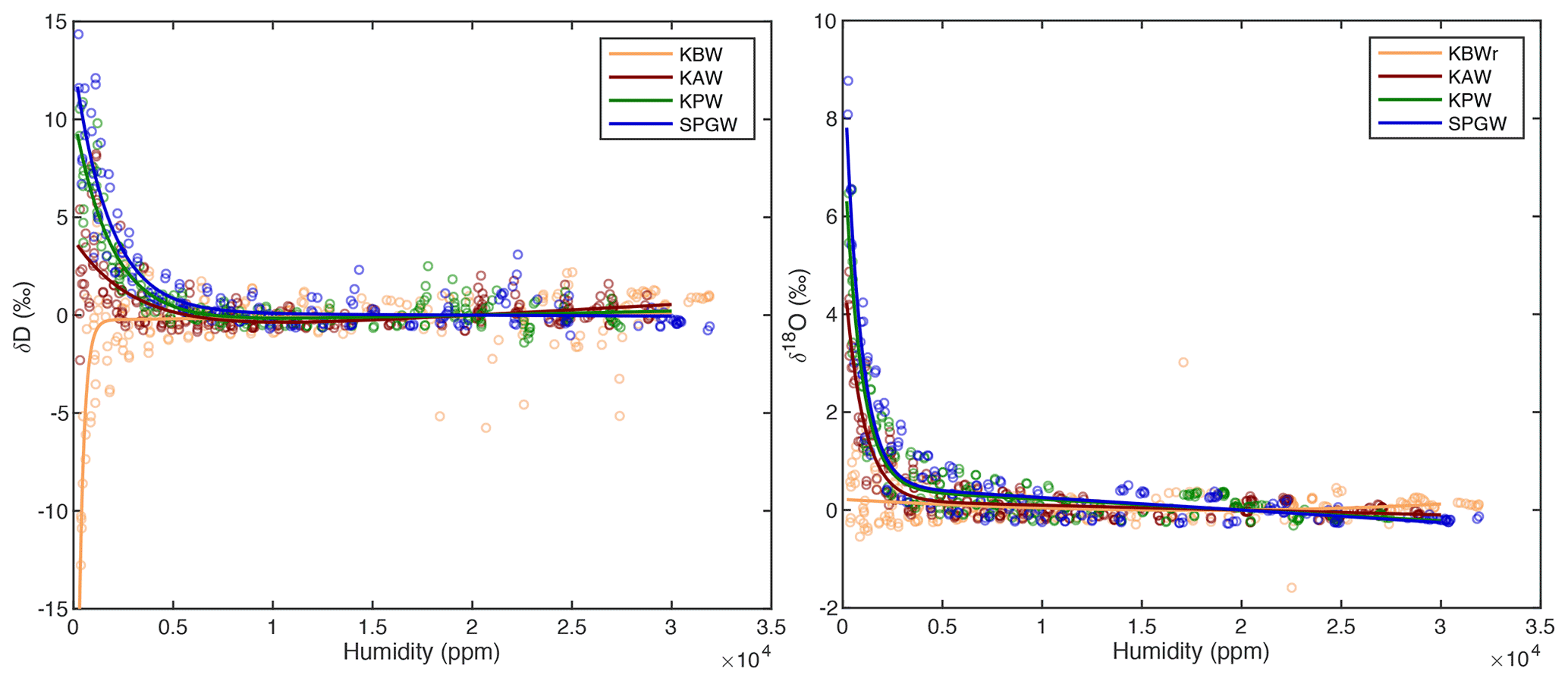
Figure A5A double exponential curve is fit to the compiled calibration data for each standard for both δ18O and δD, characterizing the instrumental humidity-isotope response. This curve, normalized to the isotope value at 20 000 ppm, is used to correct the measured isotope data for bias at low humidity values.

Figure A6The true values of standards on the VSMOW-SLAP scale are compared to a compilation of standards measured across the field season, to yield a linear relationship for (a) δ18O and (b) d-excess. This correction is applied to measured isotope data.
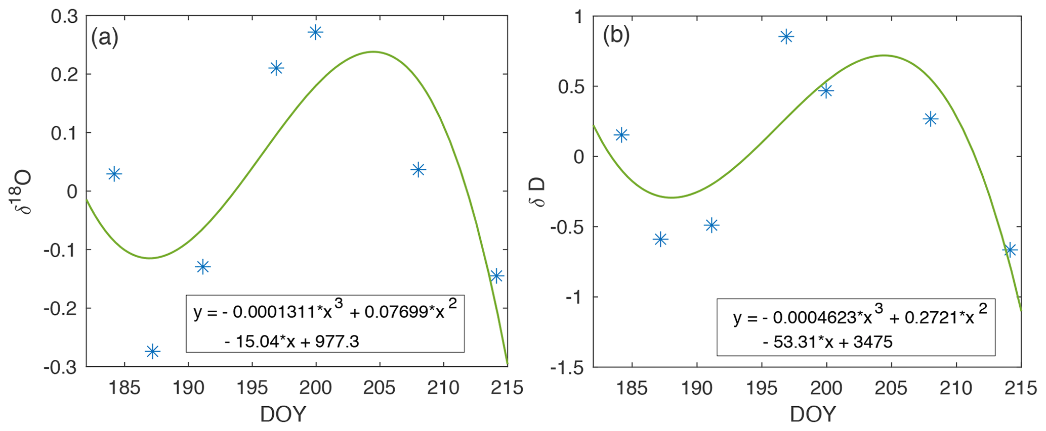
Figure A7Drift in isotope measurements across the 2019 EGRIP field season (blue). The cubic polynomial curve fit (green) is used to correct experimental vapor measurements for the associated periods of time.

Figure A8Sublimation rate with time for each laboratory experiment (L1–L8). The sublimation rate varies with temperature and dry air flow rate and is relatively constant with time throughout each experiment.
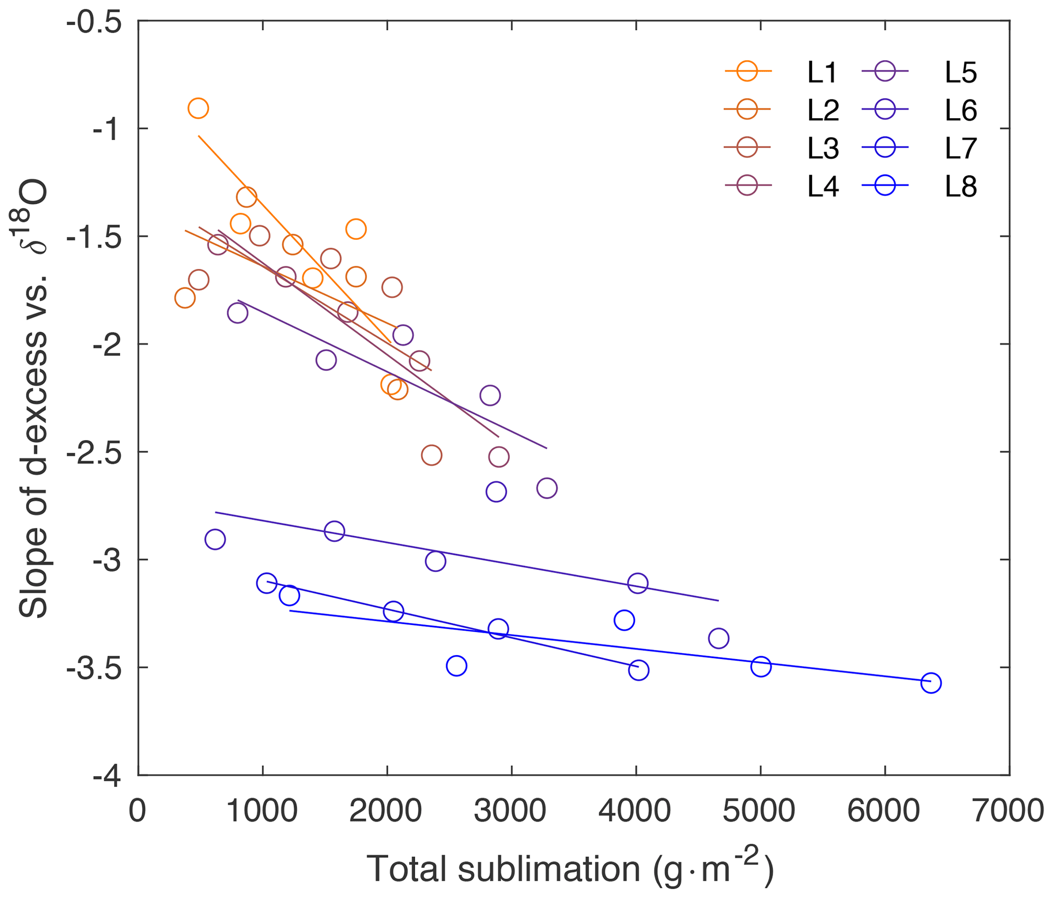
Figure A9Slope of d-excess vs. δ18O (as shown in Fig. 3) in comparison to total sublimation (sublimation rate times hours).
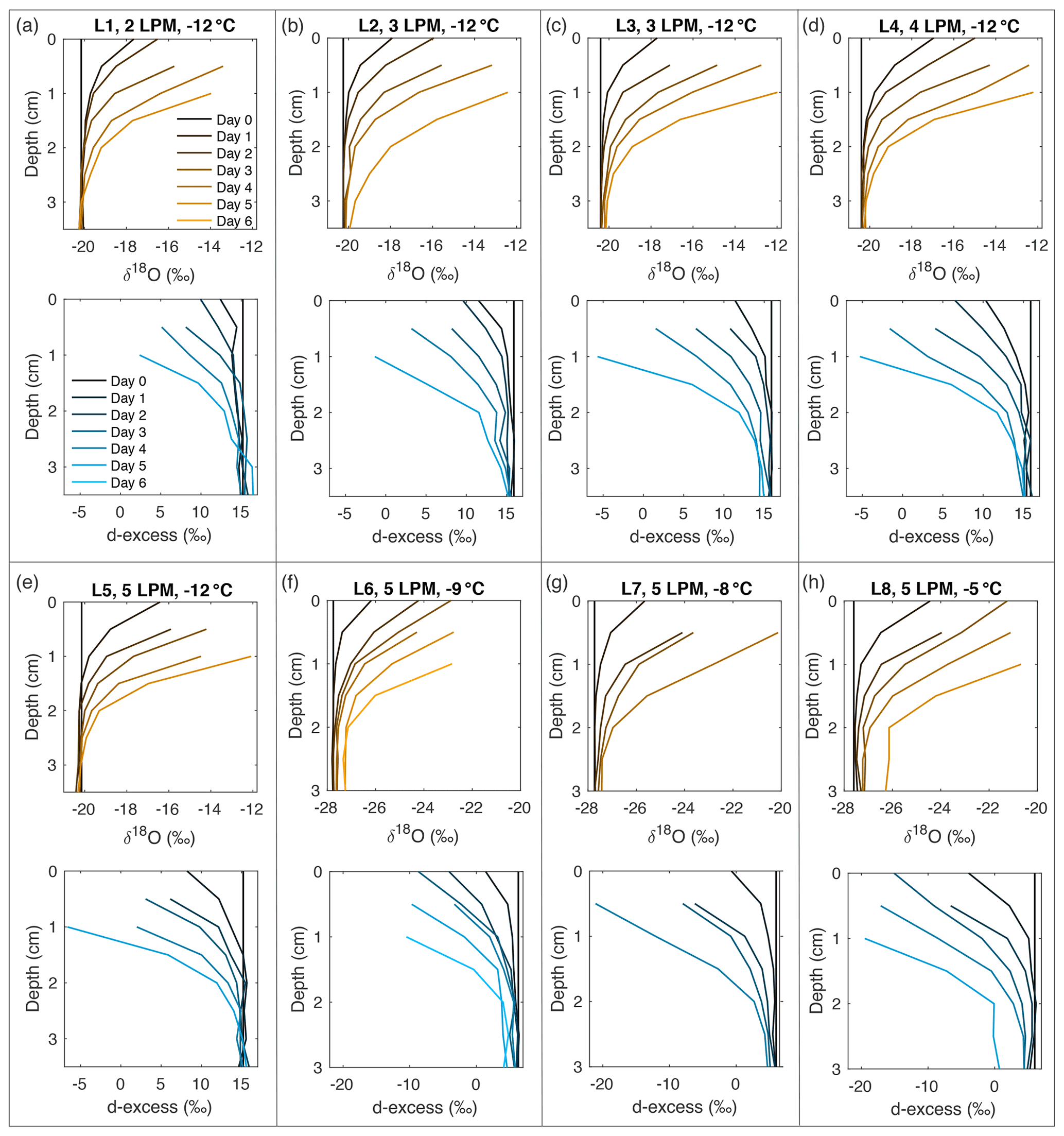
Figure A10Snow δ18O (orange) and d-excess (blue) vertical profiles from all laboratory experiments (L1–L8, (a–h), respectively). Conditions for each experiment are indicated in each subplot. Day 0 (black) represents the initial homogeneous snow sample, with colors progressively moving towards orange (δ18O) and blue (d-excess) with each day of sampling. As each experiment progresses from Day 1 to Day 6, sublimation drives an increase in δ18O and decrease in d-excess, with the greatest change at the snow surface.

Figure A11Mean daily (a) δ18O and (b) d-excess with time for laboratory experiments L1–L8. The slope of the line for each experiment is represented in (c), compared to sublimation rate. There is a slight increase in δ18O slope vs. sublimation rate (R2=0.13), with a stronger relationship observed in the decrease in d-excess vs. sublimation rate (R2=0.54).

Figure A12All surface samples are shown for field experiments FS1–FS4 (top to bottom, respectively), including δ18O (left column) and d-excess (right column). Symbols represent sampling locations (diamond, Site A; plus, Site B; asterisk, Site C), and colors indicate sampling height (yellow, 0–0.5 cm from surface; red, 0–1 cm; purple, 1–2 cm; blue, 2–4 cm). Solid lines are the average of the three sampling locations (A, B, C).
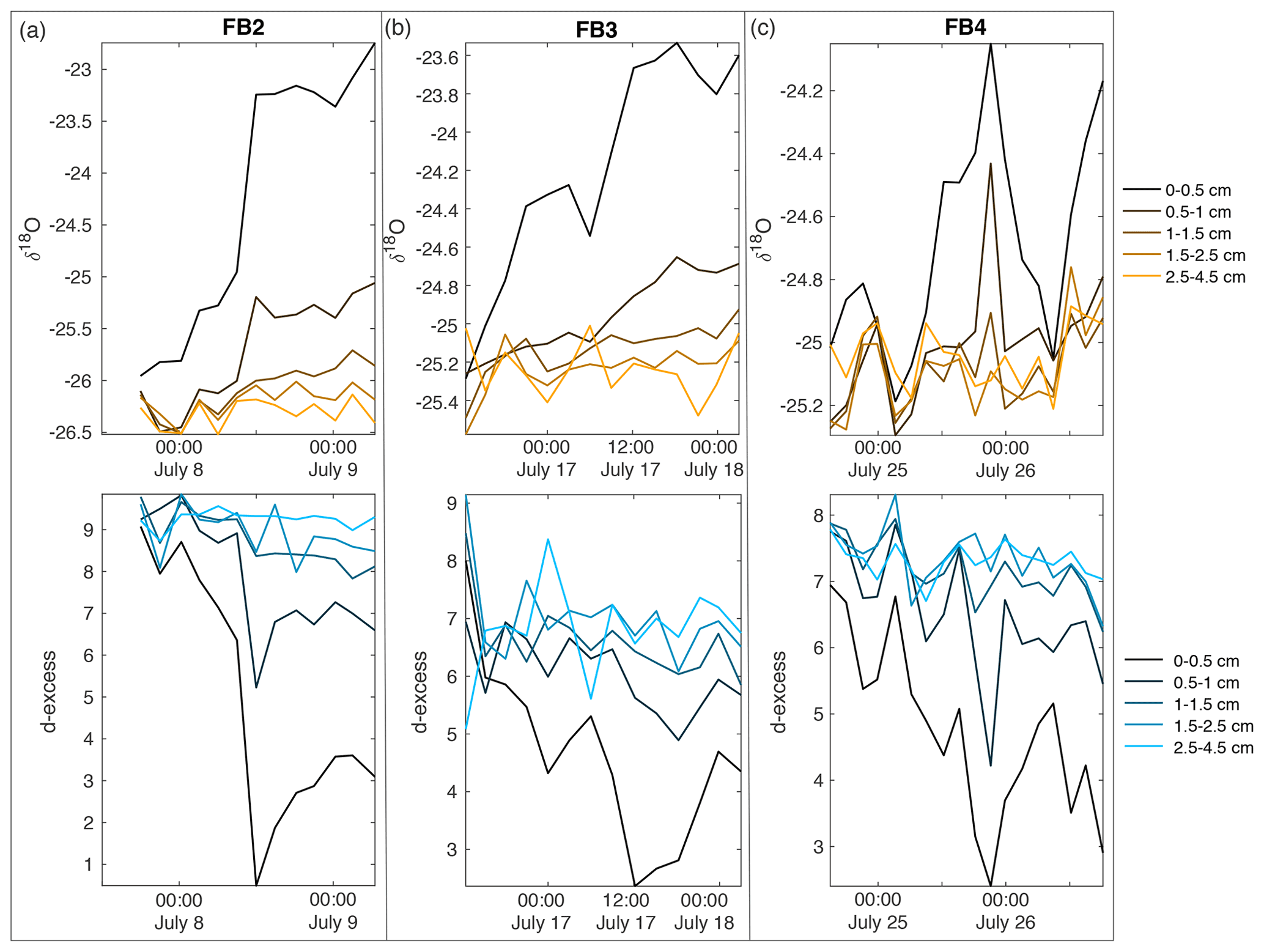
Figure A13Field box samples are shown for (a) FB2, (b) FB3, and (c) FB4, including δ18O (top row) and d-excess (bottom row). Colors indicate sampling depth from surface; black is the surface sample from 0–0.5 cm, progressing with depth towards light orange (δ18O) and light blue (d-excess) at 2.5–4.5 cm below the surface.

Figure A14Additional atmospheric conditions are shown for all field experiments F1–F4 (a–d, respectively). From top: latent heat flux (red, positive values; blue, negative values; dashed gray line at 0), temperature (orange), and atmospheric vapor measurements at 10 cm above the snow surface. Humidity (purple), δ18O (green), and d-excess (teal).
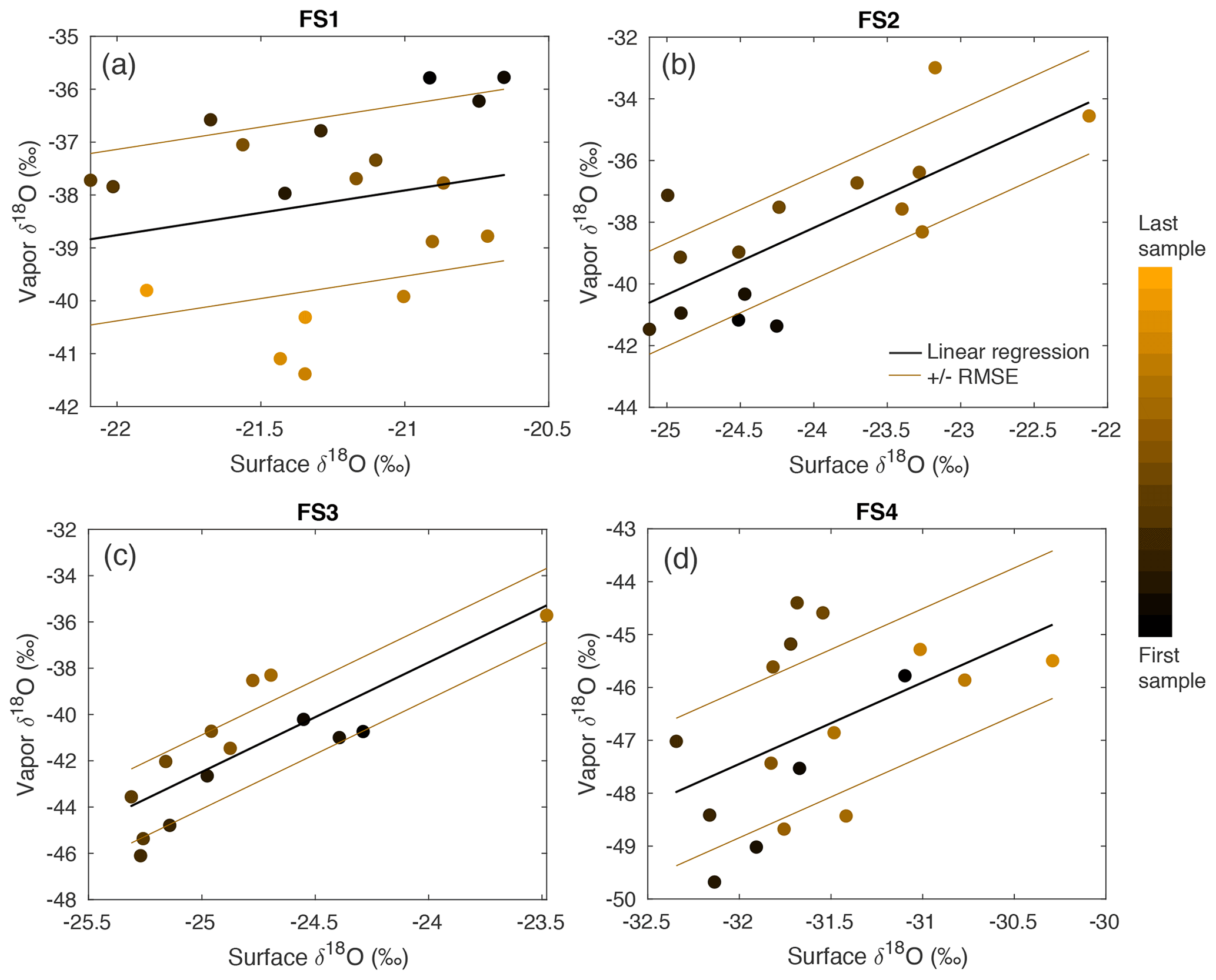
Figure A15A comparison between δ18O of vapor and the top (0–0.5 cm) FS sample shows a significant relationship in FS2, FS3, and FS4, determined by P values ≤ 0.05. The sampling time is indicated by a color scale from black (first sample taken) to orange (last sample taken), and a linear regression (black line) is calculated for each experiment. The linear regression the root-mean-square error is shown as brown lines.
The following four types of calibrations were performed to calibrate the water vapor isotope measurements of the CRDS, similar to the calibration protocol described in Steen-Larsen et al. (2013): (1) humidity, (2) humidity-isotope, (3) VSMOW-VSLAP, and (4) drift. For all isotope calibrations in both laboratory and field setups, the liquid standard was first vaporized using a nebulizer system, which produced vapor at 20 000–25 000 ppm. This vapor was combined with a dry air source using an open split, and a mass flow controller regulated the flow of dry air ranging from 10–21 cc min−1. The CRDS inlet constantly pulled a vacuum at 30 cc min−1; therefore, the remaining air flow is pulled from the humidified nebulizer source. This allowed for a constant stream of vapor at a controlled isotopic value and humidity level.
The calibration runs performed before and after each field experiment consisted of a 7 h cycle with each of the four standards (Table A1) measured for 12 min at eight different humidity levels from 500–12000 ppm, as well as a half-hour measurement at >20 000 ppm (Fig. A3). This calibration was performed before and after each field experiment run (Fig. A4). Vapor measurements have uncertainty of 0.23 ‰ δ18O and 1.4 ‰ δD (Steen-Larsen et al., 2013). Details of each laboratory and field calibration type are as follows.
-
Humidity calibration. The measured humidity was corrected to the true humidity using a polynomial relationship, which was determined by calibration to a range of known humidity levels (Fig. A2). This instrument-specific relationship was not expected to significantly drift with time.
- a.
Laboratory. A laboratory humidity calibration was carried out by drawing humid air through a chilled ethanol bath, calculating the true humidity based on the saturation vapor pressure of the bath temperature (Fig. A2).
- b.
Field. The humidity calibration required a full laboratory setup, which was not available in the field. Due to instrument damage during shipping, the calibration could not be performed after the field season. Therefore, the humidity measurements were calibrated to a second Picarro L2130-i CRDS instrument which was continuously measuring atmospheric vapor ∼30 m away and was calibrated for humidity. Simultaneous humidity measurements were matched and used to calibrate the CRDS instrument measurements reported here.
- a.
-
Humidity-isotope response calibrations. Isotopic bias occurs at a lower humidity level (i.e., less than 10 000 ppm) and is sensitive to isotope concentration (Weng et al., 2020). Because experimental vapor measurements are typically below 5000 ppm, it is important to perform a rigorous calibration of multiple isotopic standards (Table A1) at varying humidity levels (Figs. A3, A4). A double-exponential curve is fit to the isotope response with respect to humidity (Fig. A5) and is used to correct deviations in low-humidity experimental data.
- a.
Laboratory. The humidity-isotope response was determined by a full calibration of four isotopic standards (Table A1) measured for 20–30 min at a range of humidity levels from ∼500–10 000 ppm. For experiments L1–L5, vapor measurements were calibrated to KAW, and vapor measurements in experiments L6–L8 were calibrated to NEEM. These standards were closest to the isotopic values of the vapor measurements, which differed between experiments due to different starting snow isotopic composition.
- b.
Field. All calibration runs performed before and after each experiment run were compiled for the full field season. A double-exponential curve was fit to the compilation of data for each standard to determine the mean instrument response to humidity (Fig. A5). The vapor measurements were calibrated using the mean curve for KPW, which has the closest isotope value to average vapor measurements.
- a.
-
VSMOW-SLAP scale calibration. The calibration to the VSMOW-SLAP scale was established using standards (Table A1) which bracketed the measured water vapor isotope data (Fig. A6). A linear relationship is calculated between the “True value”, or the established isotopic standard value, and the “Measured value”, which is calculated from standard measurements.
- a.
Laboratory. The “Measured values” for the VSMOW-VSLAP scale were taken from the isotopic values at ∼6000–8000 ppm measured in the full calibration used for the humidity-isotope response curve.
- b.
Field. The “Measured values” were derived from the mean value of each standard measured for >10 min at 20 000–35 000 ppm over the course of the field season.
- a.
-
Drift calibration. While points (2) and (3) above account for mean instrument isotope deviations from standard values, instrument drift with time has also been observed in CRDS. For this reason, we calculated a best fit with respect to time for the isotope values at higher humidities from each calibration performed (Fig. A7). Deviations from the mean are then corrected for within each experiment period.
- a.
Laboratory. A short calibration of three to four standards at three to four humidity levels was completed before and after each experiment run. Instrument drift was calculated from the variability in KAW (L1–L5) and NEEM (L6–L8) at 2000 ppm.
- b.
Field. The isotope drift with respect to time was calculated from the mean value of measurements at 20 000 ppm for each calibration.
- a.
Latent heat flux data are available on the PANGAEA data archive at https://doi.org/10.1594/PANGAEA.928827 (Steen-Larsen and Wahl, 2021). Laboratory and field experimental data are available at https://doi.pangaea.de/10.1594/PANGAEA.937355 (Hughes, 2021).
AGH and HCSL designed the laboratory and field setup and experiments. AGH carried out the experiments with significant contributions from HCSL. SW and AZ assisted with field snow sampling, and MH assisted with materials and production ideas of the laboratory experimental chamber. AGH wrote the article with significant contributions from HCSL, TRJ, and SW and edits from all authors.
The authors declare that they have no conflict of interest.
Publisher's note: Copernicus Publications remains neutral with regard to jurisdictional claims in published maps and institutional affiliations.
Abigail Hughes acknowledges support from the National Science Foundation through the Graduate Research Fellowship Program (grant no. DGE 1650115). This paper has received funding from the European Research Council (ERC) under the European Union's Horizon 2020 research and innovation program: Starting Grant SNOWISO (grant agreement no. 759526). EGRIP is directed and organized by the Centre for Ice and Climate at the Niels Bohr Institute, University of Copenhagen. It is supported by funding agencies and institutions in Denmark (A. P. Møller Foundation, University of Copenhagen), USA (US National Science Foundation, Office of Polar Programs), Germany (Alfred Wegener Institute, Helmholtz Centre for Polar and Marine Research), Japan (National Institute of Polar Research and Arctic Challenge for Sustainability), Norway (University of Bergen and Trond Mohn Foundation), Switzerland (Swiss National Science Foundation), France (French Polar Institute Paul-Emile Victor, Institute for Geosciences and Environmental research), Canada (University of Manitoba) and China (Chinese Academy of Sciences and Beijing Normal University). Funding has also been provided by the National Science Foundation program of Arctic Natural Sciences (grant no. 1804098). The authors also thank the Stable Isotope Lab at the University of Colorado Boulder for facility and instrument use, and Bruce Vaughn and Valerie Morris for assistance.
This research has been supported by the Horizon 2020 (grant no. SNOWISO (759526)) and the National Science Foundation (grant nos. 1804098 and 1650115).
This paper was edited by Joel Savarino and reviewed by three anonymous referees.
Benson, L. V. and White, J. W. C.: Stable isotopes of oxygen and hydrogen in the Truckee River-Pyramid Lake surface-water system, 3. Source of water vapor overlying Pyramid Lake, Limnol. Oceanogr., 39, 1945–1958, 1994. a
Casado, M., Landais, A., Picard, G., Münch, T., Laepple, T., Stenni, B., Dreossi, G., Ekaykin, A., Arnaud, L., Genthon, C., Touzeau, A., Masson-Delmotte, V., and Jouzel, J.: Archival processes of the water stable isotope signal in East Antarctic ice cores, The Cryosphere, 12, 1745–1766, https://doi.org/10.5194/tc-12-1745-2018, 2018. a, b, c, d, e
Casado, M., Münch, T., and Laepple, T.: Climatic information archived in ice cores: impact of intermittency and diffusion on the recorded isotopic signal in Antarctica, Clim. Past, 16, 1581–1598, https://doi.org/10.5194/cp-16-1581-2020, 2020. a
Craig, H.: Isotopic variations in meteoric waters, Science, 133, 1702–1703, https://doi.org/10.1126/science.133.3465.1702, 1961. a
Cuffey, K. M. and Steig, E. J.: Isotopic diffusion in polar firn: implications for interpretation of seasonal climate parameters in ice-core records, with emphasis on central Greenland, J. Glaciol., 44, 273–284, 1998. a
Dansgaard, W.: Stable isotopes in precipitation, Tellus, 16, 436–468, https://doi.org/10.3402/tellusa.v16i4.8993, 1964. a, b
Dansgaard, W., Johnsen, S., Clausen, H., and Gundestrup, N.: Stable isotope glaciology, Meddelelser om Gronland, 197, 1–53, 1973. a, b
Ebner, P. P., Steen-Larsen, H. C., Stenni, B., Schneebeli, M., and Steinfeld, A.: Experimental observation of transient δ18O interaction between snow and advective airflow under various temperature gradient conditions, The Cryosphere, 11, 1733–1743, https://doi.org/10.5194/tc-11-1733-2017, 2017. a, b
Ekaykin, A. A., Hondoh, T., Lipenkov, V. Y., and Miyamoto, A.: Post-depositional changes in snow isotope content: preliminary results of laboratory experiments, Clim. Past Discuss., 5, 2239–2267, https://doi.org/10.5194/cpd-5-2239-2009, 2009. a
Fudge, T. J., Markle, B. R., Cuffey, K. M., Buizert, C., Taylor, K. C., Steig, E. J., Waddington, E. D., Conway, H., and Koutnik, M.: Variable relationship between accumulation and temperature in West Antarctica for the past 31,000 years, Geophys. Res. Lett., 43, 3795–3803, https://doi.org/10.1002/2016GL068356, 2016. a
Furukawa, R., Uemura, R., Fujita, K., Sjolte, J., Yoshimura, K., Matoba, S., and Iizuka, Y.: Seasonal-Scale Dating of a Shallow Ice Core From Greenland Using Oxygen Isotope Matching Between Data and Simulation, J. Geophys. Res.-Atmos., 122, 10873–10887, https://doi.org/10.1002/2017JD026716, 2017. a
Thayer, A.: Snow experiments EGRIP lab and field experiment data, PANGAEA [data set], https://doi.pangaea.de/10.1594/PANGAEA.937355, 2021. a
Hughes, A. G., Jones, T. R., Vinther, B. M., Gkinis, V., Stevens, C. M., Morris, V., Vaughn, B. H., Holme, C., Markle, B. R., and White, J. W. C.: High-frequency climate variability in the Holocene from a coastal-dome ice core in east-central Greenland, Clim. Past, 16, 1369–1386, https://doi.org/10.5194/cp-16-1369-2020, 2020. a, b
Johnsen, S. J., Clausen, H. B., Cuffey, K. M., Hoffmann, G., Schwander, J., and Creyts, T.: Diffusion of stable isotopes in polar firn and ice: the isotope effect in firn diffusion, Physics of Ice Core Records, 121–140, 2000. a
Johnsen, S. J., Dahl-jensen, D., Gundestrup, N., Steffensen, J. P., Clausen, H. B., Miller, H., Masson-Delmotte, V., Sveinbjo, A. E., Sveinbjörnsdóttir, Á. E., and White, J.: Oxygen isotope and palaeotemperature records from six Greenland ice-core stations: Camp Century, Dye-3, GRIP, GISP2, Renland and NorthGRIP, J. Quaternary Sci., 16, 299–307, https://doi.org/10.1002/jqs.622, 2001. a
Jones, T., Cuffey, K., White, J., Steig, E., Buizert, C., Markle, B., McConnell, J., and Sigl, M.: Water isotope diffusion in the WAIS Divide ice core during the Holocene and last glacial, J. Geophys. Res.-Earth, 122, 290–309, https://doi.org/10.1002/2016JF003938, 2017a. a
Jones, T. R., White, J. W. C., Steig, E. J., Vaughn, B. H., Morris, V., Gkinis, V., Markle, B. R., and Schoenemann, S. W.: Improved methodologies for continuous-flow analysis of stable water isotopes in ice cores, Atmos. Meas. Tech., 10, 617–632, https://doi.org/10.5194/amt-10-617-2017, 2017b. a
Jouzel, J. and Merlivat, L.: Deuterium and Oxygen 18 in Precipitation: Modeling of the Isotopic Effects During Snow Formation, J. Geophys. Res., 89, 11749–11757, 1984. a
Jouzel, J., Alley, R. B., Cuffey, K. M., Dansgaard, W., Grootes, G., Hoffmann, P., Johnsen, S. J., Koster, R. D., Peel, D., Shuman, C. A., Stievenard, M., Stuiver, M., and White, J.: Validity of the temperature reconstruction from water isotopes in ice cores, J. Geophys. Res., 102, 26471–26487, 1997. a
Laepple, T., Hörhold, M., Münch, T., Freitag, J., Wegner, A., and Kipfstuhl, S.: Layering of surface snow and firn at Kohnen Station, Antarctica: Noise or seasonal signal?, J. Geophys. Res.-Earth, 121, 1849–1860, https://doi.org/10.1002/2016JF003919, 2016. a
Laepple, T., Münch, T., Casado, M., Hoerhold, M., Landais, A., and Kipfstuhl, S.: On the similarity and apparent cycles of isotopic variations in East Antarctic snow pits, The Cryosphere, 12, 169–187, https://doi.org/10.5194/tc-12-169-2018, 2018. a
Madsen, M. V., Steen-Larsen, H. C., Hörhold, M., Box, J., Berben, S. M., Capron, E., Faber, A.-K., Hubbard, A., Jensen, M. F., Jones, T. R., Kipfstuhl, S., Koldtoft, I., Pillar, H. R., Vaughn, B. H., Vladimirova, D., and Dahl-Jensen, D.: Evidence of Isotopic Fractionation During Vapor Exchange Between the Atmosphere and the Snow Surface in Greenland, J. Geophys. Res.-Atmos., 124, 2932–2945, https://doi.org/10.1029/2018JD029619, 2019. a, b, c
Merlivat, L. and Jouzel, J.: Global Climatic Interpretation of the Deuterium-Oxygen 18 Relationship for Precipitation, J. Geophys. Res., 84, 5029–5033, 1979. a, b
Mosley-Thompson, E., Paskievitch, J. F., Gow, A. J., and Thompson, L. G.: Late 20th Century increase in South Pole snow accumulation, J. Geophys. Res.-Atmos., 104, 3877–3886, https://doi.org/10.1029/1998JD200092, 1999. a
Münch, T. and Laepple, T.: What climate signal is contained in decadal- to centennial-scale isotope variations from Antarctic ice cores?, Clim. Past, 14, 2053–2070, https://doi.org/10.5194/cp-14-2053-2018, 2018. a, b
Münch, T., Kipfstuhl, S., Freitag, J., Meyer, H., and Laepple, T.: Constraints on post-depositional isotope modifications in East Antarctic firn from analysing temporal changes of isotope profiles, The Cryosphere, 11, 2175–2188, https://doi.org/10.5194/tc-11-2175-2017, 2017. a, b
Persson, A., Langen, P. L., Ditlevsen, P., and Vinther, B. M.: The influence of precipitation weighting on interannual variability of stable water isotopes in Greenland, J. Geophys. Res.-Atmos., 116, D20120, https://doi.org/10.1029/2010JD015517, 2011. a
Ritter, F., Steen-Larsen, H. C., Werner, M., Masson-Delmotte, V., Orsi, A., Behrens, M., Birnbaum, G., Freitag, J., Risi, C., and Kipfstuhl, S.: Isotopic exchange on the diurnal scale between near-surface snow and lower atmospheric water vapor at Kohnen station, East Antarctica, The Cryosphere, 10, 1647–1663, https://doi.org/10.5194/tc-10-1647-2016, 2016. a, b
Schauer, A. J., Schoenemann, S. W., and Steig, E. J.: Routine high-precision analysis of triple water-isotope ratios using cavity ring-down spectroscopy, Rapid Commun. Mass. Sp., 30, 2059–2069, https://doi.org/10.1002/rcm.7682, 2016. a
Sime, L. C., Hopcroft, P. O., and Rhodes, R. H.: Impact of abrupt sea ice loss on Greenland water isotopes during the last glacial period, P. Natl. Acad. Sci. USA, 116, 4099–4104, https://doi.org/10.1073/pnas.1807261116, 2019. a
Sokratov, S. A. and Golubev, V. N.: Snow isotopic content change by sublimation, J. Glaciol., 55, 823–828, 2009. a
Steen-Larsen, H. C. and Wahl, S.: 2 m processed sensible and latent heat flux, friction velocity and stability at EastGRIP site on Greenland Ice Sheet, summer 2019, PANGAEA [data set], https://doi.org/10.1594/PANGAEA.928827, 2021. a
Steen-Larsen, H. C., Johnsen, S. J., Masson-Delmotte, V., Stenni, B., Risi, C., Sodemann, H., Balslev-Clausen, D., Blunier, T., Dahl-Jensen, D., Ellehøj, M. D., Falourd, S., Grindsted, A., Gkinis, V., Jouzel, J., Popp, T., Sheldon, S., Simonsen, S. B., Sjolte, J., Steffensen, J. P., Sperlich, P., Sveinbjörnsdóttir, A. E., Vinther, B. M., and White, J. W. C.: Continuous monitoring of summer surface water vapor isotopic composition above the Greenland Ice Sheet, Atmos. Chem. Phys., 13, 4815–4828, https://doi.org/10.5194/acp-13-4815-2013, 2013. a, b, c
Steen-Larsen, H. C., Masson-Delmotte, V., Hirabayashi, M., Winkler, R., Satow, K., Prié, F., Bayou, N., Brun, E., Cuffey, K. M., Dahl-Jensen, D., Dumont, M., Guillevic, M., Kipfstuhl, S., Landais, A., Popp, T., Risi, C., Steffen, K., Stenni, B., and Sveinbjörnsdottír, A. E.: What controls the isotopic composition of Greenland surface snow?, Clim. Past, 10, 377–392, https://doi.org/10.5194/cp-10-377-2014, 2014. a, b, c, d
Stevens, C. M., Verjans, V., Lundin, J. M. D., Kahle, E. C., Horlings, A. N., Horlings, B. I., and Waddington, E. D.: The Community Firn Model (CFM) v1.0, Geosci. Model Dev., 13, 4355–4377, https://doi.org/10.5194/gmd-13-4355-2020, 2020. a
Touzeau, A., Landais, A., Morin, S., Arnaud, L., and Picard, G.: Numerical experiments on vapor diffusion in polar snow and firn and its impact on isotopes using the multi-layer energy balance model Crocus in SURFEX v8.0, Geosci. Model Dev., 11, 2393–2418, https://doi.org/10.5194/gmd-11-2393-2018, 2018. a
Wahl, S., Steen-Larsen, H. C., Reuder, J., and Hörhold, M.: Quantifying the Stable Water Isotopologue Exchange Between the Snow Surface and Lower Atmosphere by Direct Flux Measurements, J. Geophys. Res.-Atmos., 126, e2020JD034400, https://doi.org/10.1029/2020JD034400, 2021. a, b, c
Weng, Y., Touzeau, A., and Sodemann, H.: Correcting the impact of the isotope composition on the mixing ratio dependency of water vapour isotope measurements with cavity ring-down spectrometers, Atmos. Meas. Tech., 13, 3167–3190, https://doi.org/10.5194/amt-13-3167-2020, 2020. a
Werner, M., Mikolajewicz, U., Heimann, M., and Hoffmann, G.: Borehole versus isotope temperatures on Greenland: Seasonality does matter, Geophys. Res. Lett., 27, 723–726, 2000. a, b
Werner, M., Langebroek, P. M., Carlsen, T., Herold, M., and Lohmann, G.: Stable water isotopes in the ECHAM5 general circulation model: Toward high-resolution isotope modeling on a global scale, J. Geophys. Res.-Atmos., 116, D15109, https://doi.org/10.1029/2011JD015681, 2011. a
Whillans, I. and Grootes, P.: Isotopic diffusion in cold snow and firn, J. Geophys. Res., 90, 3910–3918, https://doi.org/10.1029/JD090iD02p03910, 1985. a
Zuhr, A. M., Münch, T., Steen-Larsen, H. C., Hörhold, M., and Laepple, T.: Local scale depositional processes of surface snow on the Greenland ice sheet, The Cryosphere Discuss. [preprint], https://doi.org/10.5194/tc-2021-36, in review, 2021. a, b, c