Quantifying the potential future contribution to global mean sea level from the Filchner–Ronne basin, Antarctica

The future of the Antarctic Ice Sheet in response to climate warming is one of the largest sources of uncertainty in estimates of future changes in global mean sea level (ΔGMSL). Mass loss is currently concentrated in regions of warm circumpolar deep water, but it is unclear how ice shelves currently surrounded by relatively cold ocean waters will respond to climatic changes in the future. Studies suggest that warm water could flush the Filchner–Ronne (FR) ice shelf cavity during the 21st century, but the inland ice sheet response to a drastic increase in ice shelf melt rates is poorly known. Here, we use an ice flow model and uncertainty quantification approach to project the GMSL contribution of the FR basin under RCP emissions scenarios, and we assess the forward propagation and proportional contribution of uncertainties in model parameters (related to ice dynamics and atmospheric/oceanic forcing) on these projections. Our probabilistic projections, derived from an extensive sample of the parameter space using a surrogate model, reveal that the FR basin is unlikely to contribute positively to sea level rise by the 23rd century. This is primarily due to the mitigating effect of increased accumulation with warming, which is capable of suppressing ice loss associated with ocean-driven increases in sub-shelf melt. Mass gain (negative ΔGMSL) from the FR basin increases with warming, but uncertainties in these projections also become larger. In the highest emission scenario RCP8.5, ΔGMSL is likely to range from −103 to 26 mm, and this large spread can be apportioned predominantly to uncertainties in parameters driving increases in precipitation (30 %) and sub-shelf melting (44 %). There is potential, within the bounds of our input parameter space, for major collapse and retreat of ice streams feeding the FR ice shelf, and a substantial positive contribution to GMSL (up to approx. 300 mm), but we consider such a scenario to be very unlikely. Adopting uncertainty quantification techniques in future studies will help to provide robust estimates of potential sea level rise and further identify target areas for constraining projections.

1 Introduction

Ice loss from the Antarctic Ice Sheet has accelerated in recent decades (Rignot et al., 2019; Shepherd et al., 2018), and the evolution of the ice sheet in response to future climate warming is one of the largest sources of uncertainty for global mean sea level rise. Current projections suggest that the ice sheet may contribute anywhere between −7.8 and 30 cm to sea level rise by 2100 under Representative Concentration Pathway (RCP) 8.5 scenario forcing (Seroussi et al., 2020). This large spread of potential sea level rise is primarily due to uncertainties in ocean-driven thinning of ice shelves, which could initiate a positive feedback of rapid, unstable retreat and ultimate collapse of the West Antarctic Ice Sheet (Feldmann and Levermann, 2015).

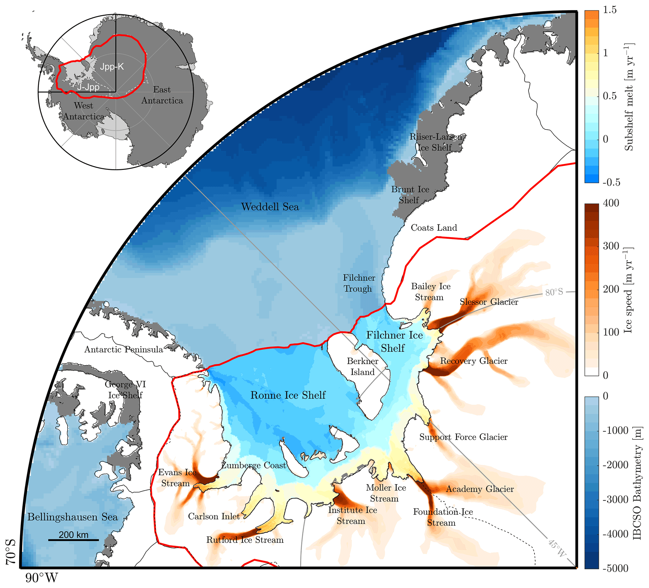
Figure 1 Map of Filchner–Ronne region. Our model domain is outlined in red. Orange to red shows model-calculated ice speeds [m yr⁻¹] initialized to observations using a model inversion with m=3 and n=3, over the grounded portion of the catchment. Blue to yellow shading shows sub-shelf melt rates across the Filchner and Ronne ice shelves, using the ocean box melt parameterization with sample point estimates for parameters from their probability distributions (see Appendix B). Light to dark blue shading shows sea floor depth from the IBCSO dataset (Arndt et al., 2013). The inset map shows the full extent of our model domain (red) as well as the drainage basins (Jpp-K, J-Jpp) as defined by Rignot et al. (2019) in white.

The Filchner–Ronne (FR) basin is a region of Antarctica that has undergone little change in recent decades and hence has not been the focus of substantial research compared to regions of Antarctica that have already begun to contribute more dramatically to sea level rise. However, the future of this region in response to climate and ocean changes remains highly uncertain. The Filchner–Ronne ice shelf (hereafter FRIS) is the second largest floating ice shelf in Antarctica, spanning approximately 400 × 10³ km² and terminating in the Weddell Sea (Fig. 1). Currently the ice shelf discharges approximately 200 Gt yr⁻¹ (Gardner et al., 2018) of sea-level-relevant ice mass into the surrounding ocean. Ice from the interior of the Antarctic Ice Sheet flows into the FRIS primarily via 11 fast-flowing ice streams (Fig. 1). These ice streams are marine-based; i.e. their bed topography rests substantially below sea level, which has implications for marine ice sheet instability (Ross et al., 2012). Throughout this paper we refer to the FR basin as the combined area of the two major drainage basins (Jpp-K, J-Jpp) as defined by Rignot et al. (2019) that encompass a number of smaller ice stream catchments that drain into the FRIS.

Current mass loss from the Antarctic Ice Sheet is concentrated in regions where warm circumpolar deep water propagates on the continental shelf (e.g. Amundsen Sea Embayment (ASE): Jacobs et al., 2011; Jenkins et al., 2010; Schmidtko et al., 2014). Warm water in the ASE has been linked to recent ice shelf thinning (Pritchard et al., 2012; Paolo et al., 2015), grounding line retreat (Rignot et al., 2014), and increased ice discharge (Mouginot et al., 2014; Shepherd et al., 2018; Rignot et al., 2019). In contrast, water entering the FRIS cavity is relatively cold (< 0 ^∘C), high-salinity shelf water, and as a result, sub-shelf melt rates are an order of magnitude lower than those in the ASE. The FR basin is also a region of Antarctica that has not undergone significant change during the modern observational period. Over the past 4 decades (1979–2017), the FR basin has remained relatively stable (accumulation is balanced by discharge) (Rignot et al., 2019), alongside a negligible change (1–3 cm yr⁻¹) in surface elevation (Shepherd et al., 2019) and no significant long-term speed-up of the major ice streams (Gudmundsson and Jenkins, 2009; Gardner et al., 2018).

Recent work suggests that melt rates beneath the FRIS could greatly increase in response to a tipping point in the neighbouring Weddell Sea. Studies have now shown that 21st century changes in atmospheric conditions and sea ice concentration could redirect relatively warm deep water beneath the FRIS via the Filchner trough (Fig. 1: Hellmer et al., 2012, 2017; Hazel and Stewart, 2020). This would cause the FR cavity to switch from what is widely referred to as a “cold state” to a “warm state”, similar to the ice shelf cavities (e.g. Pine Island and Thwaites) in the ASE. Ultimately, this warm water could be directed towards highly buttressed regions of the ice shelf close to the grounding line (Reese et al., 2018a) via deep cavity bathymetry (e.g. Foundation Ice Stream: Rosier et al., 2018) and dramatically increase melt rates under the FRIS. A loss of resistive stress at the grounding line as a result of ocean-induced melt could force dynamic imbalance and grounding line retreat of the ice streams feeding the FRIS.

Most previous studies have only assessed uncertainties in sea level contribution, on an ice-sheet-wide scale, rather than individual drainage basins (with the exception of Schlegel et al., 2018). These Antarctic-wide ensemble simulations also rely on coarse grid resolution to be computationally feasible, and as a result they may not capture small-scale processes or accurate grounding line migration relevant on regional scales. Some studies have performed sensitivity experiments on climate–ocean forcing on the FR basin (Cornford et al., 2015; Wright et al., 2014), but we do not know of an uncertainty quantification assessment of the FR region's potential contribution to sea level rise. A comprehensive uncertainty analysis is needed to fully understand the future of this region of Antarctica should it undergo an increase in sub-shelf melting.

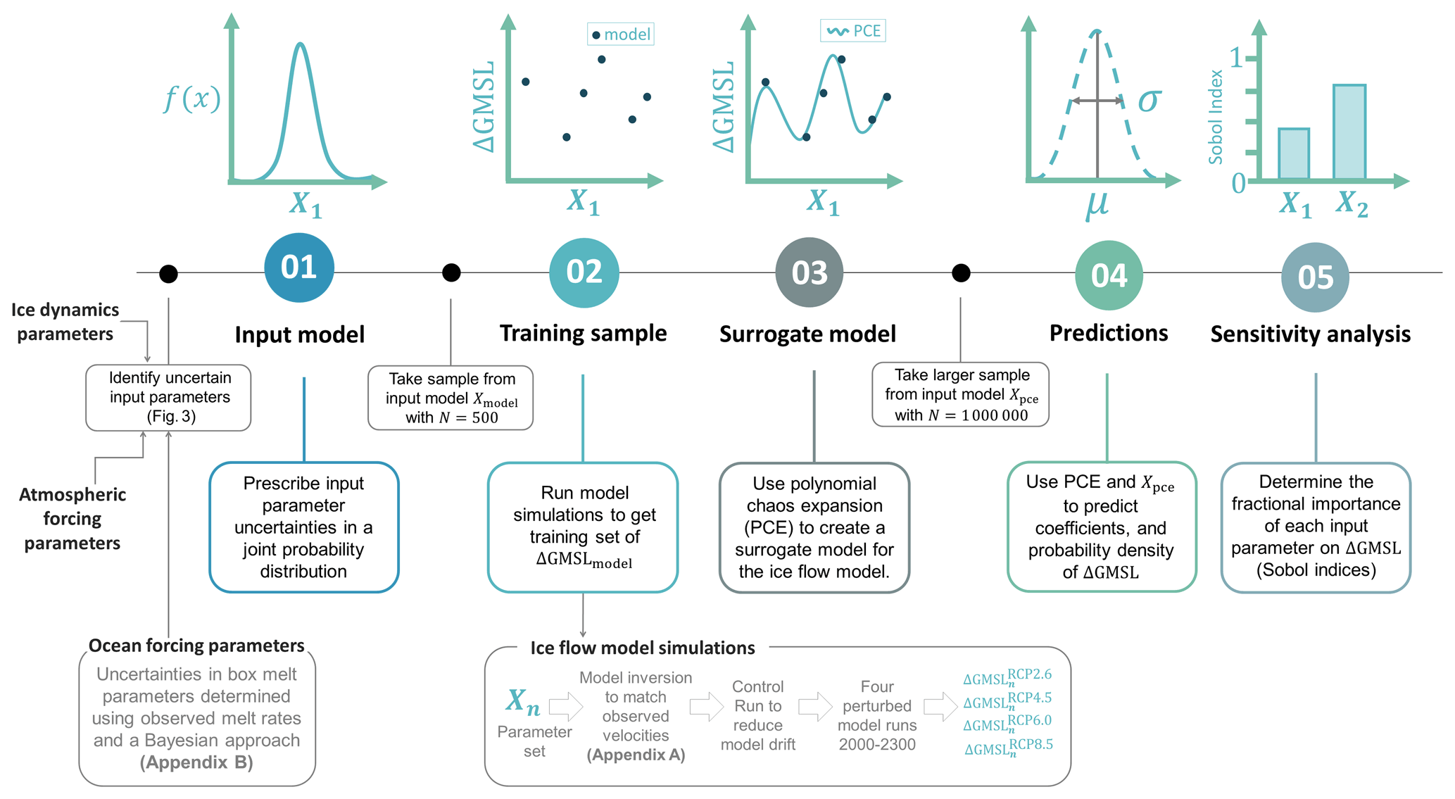
Figure 2 Workflow diagram summarizing the uncertainty quantification approach used in this study. We first identify uncertain input parameters and represent them in probabilistic framework. A training sample of 500 points is taken from this input parameter space and used as input to an ensemble of simulations in our ice flow model, which we hereafter refer to as our “training ensemble”. Using this training sample and the surrogate modelling capabilities in UQLAB we create a polynomial chaos expansion (PCE) that mimics the behaviour of our ice flow model. This allows us to evaluate a much larger sample from our parameter space, and these surrogate models are used to derive predictions and probability density functions for changes in global mean sea level (ΔGMSL). Finally, we use sensitivity analysis to identify the proportional contribution of each input parameter on projection uncertainty.

In this paper, we use an uncertainty quantification approach to assess the future of the FR basin to achieve three aims: (1) estimate potential mass change from the FR basin through to the year 2300, (2) quantify the uncertainty associated with mass change projections, and (3) identify parameters in our model or forcing functions that account for the majority of our projection uncertainty and should be priority areas for further research to constrain the spread of future projections. To do this, we integrate an existing suite of uncertainty quantification tools (UQLAB: Marelli and Sudret, 2014) for use with the state-of-the-art ice flow model Úa (Gudmundsson, 2020). See Fig. 2 for a summary of the method used in this paper. The paper is structured as follows: in the following (Sect. 2) we introduce the uncertainty methodology used in this paper. In Sect. 3 we explain the model set-up and input parameters that are propagated through our forward model. Section 4 presents our probabilistic projections and the results of our sensitivity analysis, which are then discussed in Sect. 5.

2 Uncertainty quantification

Uncertainty quantification can be broadly defined as the science of identifying sources of uncertainty and determining their propagation through a model or real-world experiment with the ultimate goal of quantifying, in probabilistic terms, how likely an outcome or quantity of interest may be.

Early estimates of uncertainties in projections of future sea level change from the Antarctic Ice Sheet were derived from sensitivity studies that evaluated a small sample of a parameter space directly in individual ice sheet models (e.g. DeConto and Pollard, 2016; Winkelmann et al., 2012; Golledge et al., 2015; Ritz et al., 2015). Model intercomparison experiments have since been used to quantify uncertainties associated with differences in the implementation of physical processes between models, beginning with idealized set-ups (e.g. MISMIP and MISMIP+; Pattyn et al., 2012; Cornford et al., 2015), and more recently on an ice sheet scale as part of the ISMIP6 project (Seroussi et al., 2020). Recently, the use of uncertainty quantification techniques has become more common for estimating uncertainties in projections of, for example, sea level rise, based on the current knowledge of uncertainties associated with model parameters or forcing functions (parametric uncertainty) (Edwards et al., 2019; Schlegel et al., 2018, 2015; Bulthuis et al., 2019; Aschwanden et al., 2019; Nias et al., 2019; Wernecke et al., 2020). This includes techniques that weight model parameters and outputs according to some performance measures, to provide a probabilistic assessment of sea level change (Pollard et al., 2016; Ritz et al., 2015). Some of these studies have also drawn upon statistical surrogate modelling techniques such as Gaussian process emulators (Edwards et al., 2019; Pollard et al., 2016; Wernecke et al., 2020) or polynomial chaos expansions (Bulthuis et al., 2019) to mimic the behaviour of an ice sheet model and sample a much larger parameter space to make predictions of Antarctic contribution to sea level rise.

In this study, we are using a probabilistic approach, in which we are primarily interested in quantifying uncertainties in the forward propagation of input uncertainties that relate to parameters in the model or in the functions used to force climate warming, on a quantity of interest. We make use of the MATLAB-based toolbox, UQLab, and the uncertainty quantification framework of Sudret (2007), on which the MATLAB-based toolbox is based (Marelli and Sudret, 2014). UQLab includes an extensive suite of tools encompassing all necessary aspects of uncertainty quantification. Here, we summarize the approach and tools used in this study (Fig. 2), and we refer the reader to the UQLAB documentation (https://www.uqlab.com/, last access: 29 September 2021, Marelli and Sudret, 2014) for further details.

We can think of a physical model (ℳ) as a map from an input parameter space to an output quantity of interest, as

$$\begin{array}{}\text{(1)}& Y=\mathcal{M}\left(X\right),\end{array}$$

where our uncertain input parameters are specified as a probabilistic input model (X) with a joint probability distribution function X∼f_X(x), and Y is a list of model responses. Using this approach we are able to propagate the uncertainties in the inputs X to the outputs Y. We can think of our ice flow model in the same way, ΔGMSL = $\stackrel{\mathrm{´}}{\mathrm{U}}\mathrm{a}\left(X\right)$, where ΔGMSL is our model response or quantity of interest. In the following sections we outline eight uncertain input parameters that are represented in X. These relate to basal sliding and ice rheology (Sect. 3.2), surface accumulation (Sect. 3.3), and sub-shelf melting (Sect. 3.4). Uncertainties in these input parameters are defined in a probabilistic way based on the available information (Fig. 3). For parameters used to force sub-shelf melt rates, we conducted a separate Bayesian analysis to determine their input parameter probability distributions (see Appendix B).

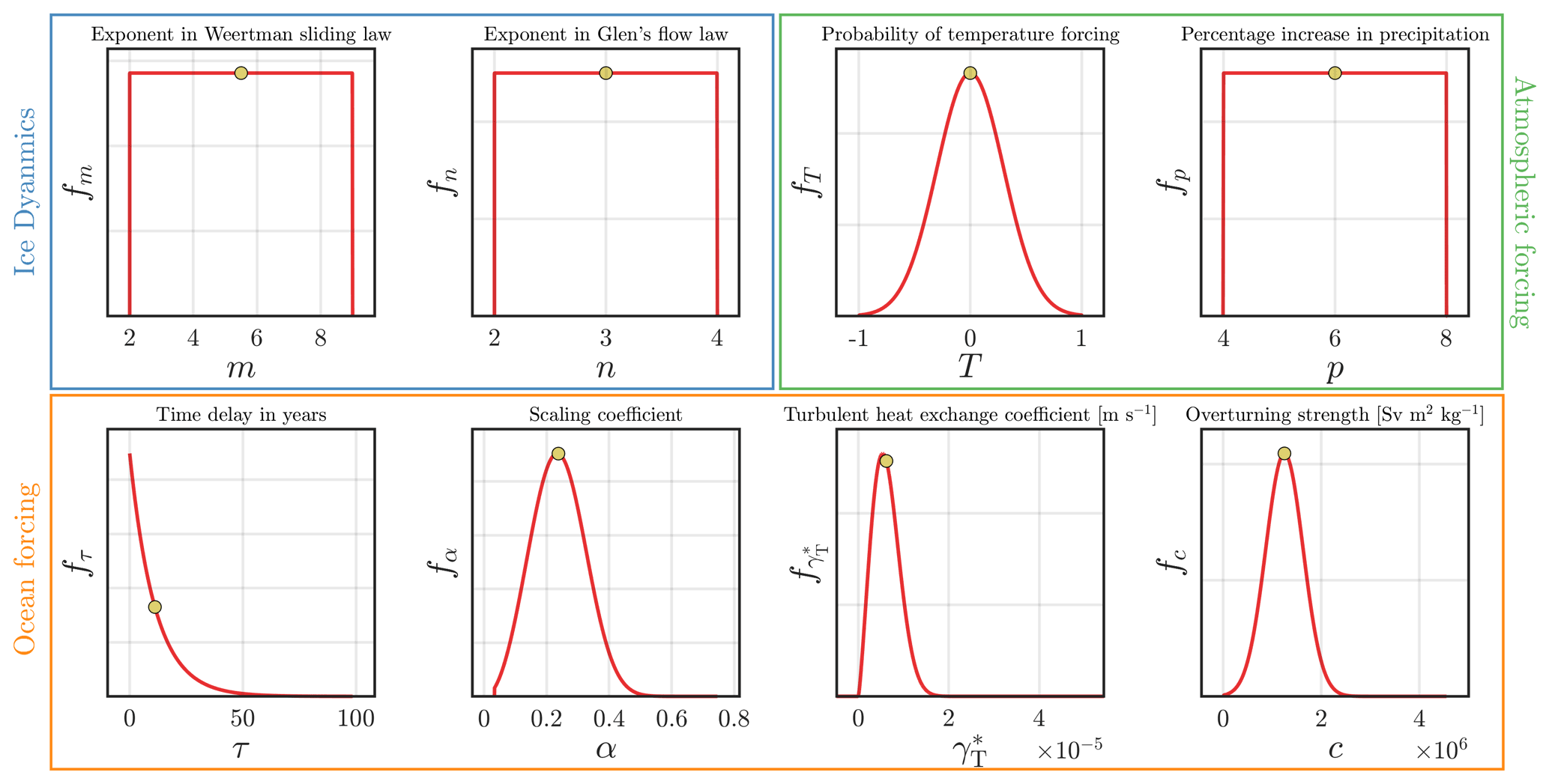
Figure 3 Probability distributions for uncertain parameters included in our analysis, grouped by ice dynamics (blue rectangle), atmospheric forcing (green rectangle), and ocean forcing (orange rectangle). For each parameter, x axes show the parameter bounds, and red lines show the probability distribution functions. Yellow circles show the sample point estimates for each of our parameters. The distributions of the four ocean forcing parameters are outputs from our Bayesian analysis (Appendix B) in which we optimized the parameter distributions using observations of melt rates beneath the Filchner–Ronne ice shelf.

Quantifying the uncertainty in model outputs due to uncertainty in input parameters or forcings may require a computationally unfeasibly large number of model evaluations. However if, for example, the model response varies slowly as the values of some input parameters are changed, the relationship between model inputs and model outputs may be approximated using a much simpler and computationally faster surrogate model. The uncertainty estimation can then be done in a much more computationally efficient way using the surrogate model.

Polynomial chaos expansion (PCE) is a surrogate modelling technique that approximates the relationship between input parameters and output response in an orthogonal polynomial basis. Aside from the work of Bulthuis et al. (2019), PCE surrogate modelling has not yet been used extensively by the glaciological community as a computationally efficient substitute for ice sheet models. The truncated PCE, ℳ^PC(X), used to approximate the behaviour of our ice sheet model ℳ(X), takes the form

$$\begin{array}{}\text{(2)}& \mathcal{M}\left(X\right)\approx {\mathcal{M}}^{\text{PC}}\left(X\right)=\sum _{\mathit{\alpha }\in \mathcal{A}}{y}_{\mathit{\alpha }}{\mathrm{\Psi }}_{\mathit{\alpha }}\left(X\right),\end{array}$$

where Ψ_α(X) represents multivariate polynomials that are orthonormal with respect to the joint input probability density function f_X, 𝒜⊂ℕ^M is a set of multi-indices of the multivariate polynomials Ψ_α, and y_α represents the coefficients. Here, our PCEs are calculated using the least angle regression (LAR) algorithm in UQLab (Blatman and Sudret, 2011; Marelli and Sudret, 2019) that solves a least-square minimization problem. This algorithm iteratively moves regressors from a candidate set to an active set, and at each iteration a leave-one-out (LOO) cross-validation error is calculated. After all iterations are complete, the best sparse candidate basis is that with the lowest leave-one-out error. This is designed to reduce the potential for over-fitting and reduced accuracy when making predictions outside of the training set. This sparse PCE calculation in UQLab also uses the LOO error for (1) adaptive calculation of the best polynomial degree based on the experimental design and (2) adaptive q-norm setup for the truncation scheme. For further details on the PCE algorithm see Marelli and Sudret (2019). We also outline details on how input uncertainties were propagated through our model to create our PCE in Sect. 3.5.

Once the surrogate model has been created, the moments of the PCE are encoded in its coefficients where the mean (μ^PC) and variance (σ^PC)² are as follows

$$\begin{array}{}\text{(3)}& {\displaystyle }{\mathit{\mu }}^{\text{PC}}=\mathbb{E}\left[{\mathcal{M}}^{\text{PC}}\right(X\left)\right]=y_{\mathrm{0}},\text{(4)}& {\displaystyle }({\mathit{\sigma }}^{\text{PC}}{)}^{\mathrm{2}}=\mathbb{E}[\left({\mathcal{M}}^{\text{PC}}\right(X)-{\mathit{\mu }}^{\text{PC}}{)}^{\mathrm{2}}]=\sum _{\begin{array}{c}\mathit{\alpha }\in \mathcal{A}\\ \mathit{\alpha }\ne \mathrm{0}\end{array}}{y}_{\mathit{\alpha }}^{\mathrm{2}}.\end{array}$$

Our existing PCE surrogate models can additionally be used in a sensitivity analysis to quantify the proportional contribution of parametric uncertainty on projections of ΔGMSL. This allows us to identify input parameters where improved understanding is needed to constrain future projections. Here, we are using Sobol indices which are a variance-based method where the model can be expanded into summands of increasing dimension, and total variance in model output can be described as the sum of the variances of these summands.

First-order indices (S_i), often also referred to as “main effects”, are the individual effect of each input parameter (X_i) on the variability in the model response (Y), defined as

$$\begin{array}{}\text{(5)}& S_i={\displaystyle \frac{\text{Var}\left[\mathbb{E}\right(Y\left|X_i\right)]}{\text{Var}\left(Y\right)}}.\end{array}$$

Total Sobol indices ($S_i^T$) are then the sum of all Sobol indices for each input parameter and encompass the effects of parameter interactions. Values for Sobol indices are between 0 and 1, where large values of S_i indicate parameters that strongly influence the projections of global mean sea level. If $S_i\approx S_i^T$, then it can be assumed that the effect of parameter interactions is negligible.

These Sobol indices can be calculated analytically from our existing PCEs, by expanding portions of the polynomial that depend on each input variable to directly calculate parameter variance using the PCE coefficients. Each of the summands of the PCE can be expressed as

$$\begin{array}{}\text{(6)}& f_v\left(x_v\right)=\sum _{\mathit{\alpha }\in {\mathcal{A}}_v}{y}_{\mathit{\alpha }}{\mathrm{\Psi }}_{\mathit{\alpha }}\left(X\right).\end{array}$$

Due to the orthonormality of the basis, the variance of our truncated PCE reads as

$$\begin{array}{}\text{(7)}& {\displaystyle }\text{Var}\left[{\mathcal{M}}^{\text{PC}}\right(X\left)\right]=\sum _{\begin{array}{c}\mathit{\alpha }\in \mathcal{A}\\ \mathit{\alpha }\ne \mathrm{0}\end{array}}{y}_{\mathit{\alpha }}^{\mathrm{2}},\text{(8)}& {\displaystyle }\text{Var}\left[f_v\right(x_v\left)\right]=\sum _{\begin{array}{c}\mathit{\alpha }\in {\mathcal{A}}_v\\ \mathit{\alpha }\ne \mathrm{0}\end{array}}{y}_{\mathit{\alpha }}^{\mathrm{2}}.\end{array}$$

The first-order Sobol indices in Eq. (5) are then calculated as the ratio between the two terms above.

3 Methods

3.1 Ice flow model

Here we use the vertically integrated ice flow model Úa (Gudmundsson, 2020) to solve the ice dynamics equations using the shallow-ice stream approximation (SSTREAM), also commonly referred to as the shallow-shelf approximation (SSA) and the “shelfy-stream” approximation. (MacAyeal, 1989). Úa has been used in previous studies on grounding line migration and ice shelf buttressing and collapse (De Rydt et al., 2015; Reese et al., 2018b; Gudmundsson et al., 2012; Gudmundsson, 2013; Hill et al., 2018), and model results have been submitted to a number of intercomparison experiments (Pattyn et al., 2008, 2012; Levermann et al., 2020; Cornford et al., 2020).

Our model domain extends across the two major drainage basins that feed into the FRIS (Fig. 1). Within this domain, we generated a finite-element mesh (Fig. S1 in the Supplement) with ∼ 92 000 nodes and ∼ 185 000 linear elements using the Mesh2D Delaunay-based unstructured mesh generator (Engwirda, 2015). Element sizes were refined based on effective strain rates and distance of the grounding line and have a maximum size of 27 km, a median size of 2 km, and a minimum size of 660 m. Within a 10 km distance of the grounding line elements are 3 km and refined further to 900 m within a distance of 1.5 km. Outside of our uncertainty analysis, we tested the sensitivity of our results to mesh resolution by repeating our median and maximum ΔGMSL simulations under RCP8.5 forcing and dividing or multiplying the aforementioned element sizes by 2. Our results are largely insensitive to the mesh resolution, with a percentage deviation in ΔGMSL of only 3 % by 2300. Finally, we linearly interpolated ice surface, thickness, and bed topography from BedMachine Antarctica v1 (Morlighem et al., 2020) onto our model mesh. We initialize our model to match observed velocities using an inverse approach (see Sect. 3.2 and Appendix A).

During forward transient simulations, Úa allows for fully implicit time integration, and the non-linear system is solved using the Newton–Raphson method. Úa includes automated time-dependent mesh refinement, allowing for high mesh resolution around the grounding line as it migrates inland. We also impose a minimum thickness constraint of 30 m using the active-set method to ensure that ice thicknesses remain positive. Throughout all simulations our calving front remains fixed in its originally prescribed position. At the end of each forward simulation we calculate the final change in global mean sea level (ΔGMSL) as the ice volume above flotation that will contribute to sea level change based on the area of the ocean (Goelzer et al., 2020).

3.2 Basal sliding and ice rheology

There are two components of surface glacier velocities: internal deformation and basal sliding. Úa uses inverse methods to optimize these velocity components based on observations by estimating the ice rate factor (A) in Glen's flow law and basal slipperiness parameter (C) in the sliding law. This section introduces uncertainties related to the exponents of the flow law and basal sliding law, whereas details of the inverse methodology are included in Appendix A.

Glen's flow law (Glen, 1955) is used to relate strain rates and stresses as a simple power relation

$$\begin{array}{}\text{(9)}& {\dot{\mathit{ϵ}}}_{ij}=A{\mathit{\tau }}_e^{n-\mathrm{1}}{\mathit{\tau }}_{ij},\end{array}$$

where ${\dot{\mathit{ϵ}}}_{ij}$ are the elements of the strain rate tensor, τ_e is effective stress (second invariant of the deviatoric stress tensor), τ_ij are the elements of the deviatoric stress tensor, A is the temperature-dependent rate factor, and n is the stress exponent.

This stress exponent (n) controls the degree of non-linearity of the flow law, and most ice flow modelling studies adopt n=3, as it is considered applicable to a number of regimes (see review in Cuffey and Paterson, 2010). However, experiments reaching high stresses (Kirby et al., 1987; Goldsby and Kohlstedt, 2001; Treverrow et al., 2012), or analysing borehole measurements and ice velocities (e.g. Gillet-Chaulet et al., 2011; Cuffey and Kavanaugh, 2011; Bons et al., 2018), have suggested that n>3. It is also possible that at low stresses, the creep regime may become more linear n<3 (Jacka, 1984; Pettit and Waddington, 2003; Pettit et al., 2011), which is supported by ice shelf spreading rates n = 2–3 (Jezek et al., 1985; Thomas, 1973). While it can be considered that n=3 is appropriate in most dynamical studies, the exact numerical value is not known and it appears plausible that it can range between 2 and 4. To capture the uncertainty in the stress exponent, we take $n\in [\mathrm{2},\mathrm{4}]$ and sample continuously from a uniform distribution within this range (Fig. 3).

Basal sliding is considered the dominant component of surface velocities in fast-flowing ice streams. The Weertman sliding law is defined as

$$\begin{array}{}\text{(10)}& {\mathit{\tau }}_b=C^{-\mathrm{1}/m}\Vert v_b{\Vert }^{\mathrm{1}/m-\mathrm{1}}{v}_b,\end{array}$$

where C is a basal slipperiness coefficient and v_b the basal sliding velocity. The Weertman sliding law typically captures hard-bed sliding, in which case m=n and is normally set equal to 3 (Cuffey and Paterson, 2010). However, using different values for m alters the non-linearity of the sliding law and can thus be used to capture different sliding processes, i.e. viscous flow for m=1 and plastic deformation for m=∞. There are limited in situ observations of basal conditions, and the value of m relies on numerical estimates of basal sliding based on model fitting to observations.

A number of studies have tested different values of m to fit observations of grounding line retreat or speed-up at Pine Island Glacier (Gillet-Chaulet et al., 2016; Joughin et al., 2010; De Rydt et al., 2021). These studies show that m=3 can underestimate observations, and more plastic-like sliding (m>3) is needed in at least some parts of the catchment to replicate observations (Joughin et al., 2010; De Rydt et al., 2021). This uncertainty in the value of m can ultimately affect projections of sea level rise (Ritz et al., 2015; Bulthuis et al., 2019; Alevropoulos-Borrill et al., 2020) by altering the length and time taken for perturbations (e.g. ice shelf thinning or grounding line retreat) to propagate inland.

While additional sliding laws have been proposed and are now implemented within a number of existing ice flow models, in this study we use the Weertman sliding law, as it remains the most common. This narrows the parameter space, allowing us to fully integrate the influence of m on projections of future sea level rise into our uncertainty assessment (by performing an inverse model run prior to each perturbed run; see Sect. 3.5). This is an advancement over previous Antarctic-wide studies, which given domain size have no choice but to invert the model for a handful of different m values prior to uncertainty propagation (e.g. Bulthuis et al., 2019; Ritz et al., 2015). To capture uncertainty in m and to sample from a range of possible methods of basal slip, we take $m\in [\mathrm{2},\mathrm{9}]$ and sample from a uniform distribution (Fig. 3).

3.3 Surface accumulation

To capture uncertainties in future climate forcing, we use projections from four Representative Concentration Pathways (RCPs) presented in the Fifth Assessment Report of the Intergovernmental Panel on Climate Change (IPCC). These pathways capture plausible changes in anthropogenic greenhouse gas emissions for the 21st and 22nd centuries. RCP2.6 is a strongly mitigated scenario, and multi-model mean estimates from the IPCC report (IPCC, 2014) project a global temperature increase of less than 2 ^∘C above pre-industrial levels by 2100 and is the goal of the 2016 Paris Agreement. Two intermediate scenarios (RCP4.5 and RCP6.0) represent global temperature increases of ∼ 2.5 and ∼ 3 ^∘C with reductions in emissions after 2040 and 2080, respectively (IPCC, 2014). Finally, RCP8.5 projects a global temperature increase of ∼ 4.5 ^∘C by 2100 and is now often referred to as an “extreme” or “worst-case” climate change scenario.

Global mean temperature changes (ΔT_g) from 1900 to 2300 relative to pre-industrial levels were obtained from the atmosphere–ocean general circulation model emulator MAGICC6.0 (http://live.magicc.org, last access: 29 September 2021: Meinshausen et al. (2011)). For each RCP scenario we obtain 600 (historically constrained) model simulations between 2000 and 2100 (see Meinshausen et al. (2009) for details on the probabilistic set-up). We then use the ensemble median and uncertainty bounds within a “very likely” range between the 25th and 75th percentiles. To extend the record to 2300, we use a single model realization, using the default climate parameter settings used to produce the RCP greenhouse gas concentrations for each RCP scenario (Meinshausen et al., 2009) and keep the upper and lower bounds constant from 2100 to 2300 (Fig. 4). Uncertainty in projections from 2100 to 2300 may well be larger, but we choose not to make an assumption on how errors will propagate up to 2300. Global temperatures from MAGICC 6.0 were also used in the Antarctic linear response model inter-comparison (LARMIP-2) experiment (Levermann et al., 2020) and are consistent with projections used in other Antarctic-wide simulations (Bulthuis et al., 2019; Golledge et al., 2015).

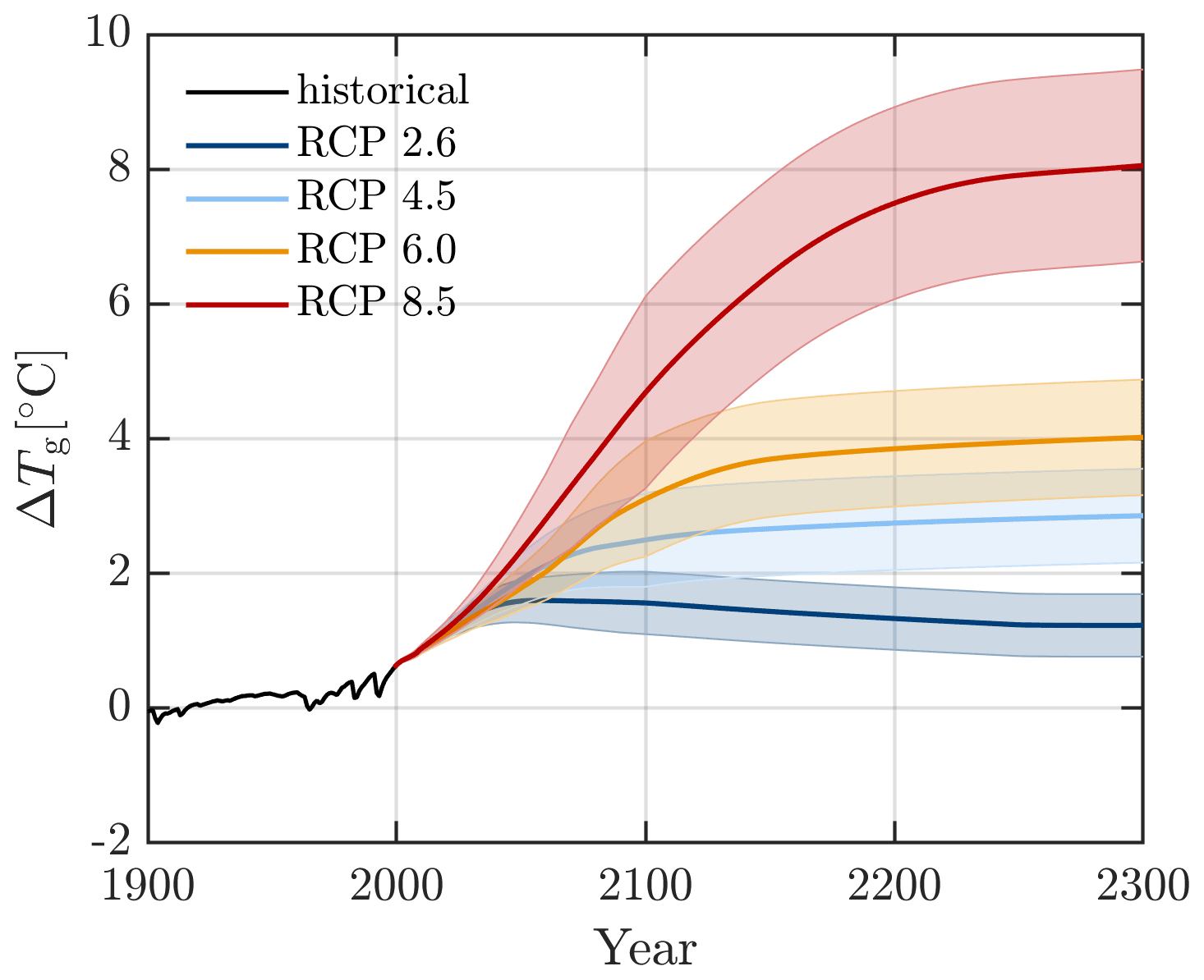
Figure 4 Changes in global mean temperatures (ΔT_g [^∘C]) relative to pre-industrial levels for four Representative Concentration Pathways (RCPs) 2.6 (blue), 4.5 (green), 6.0 (yellow), and 8.5 (pink). Shading shows uncertainty regions between the 25th and 75th percentiles.

Following the work of a number of previous studies (e.g. Pattyn, 2017; Bulthuis et al., 2019; DeConto and Pollard, 2016; Garbe et al., 2020), global temperature changes (ΔT_g) are used to force annual changes in surface mass balance through our forward-in-time simulations, by prescribing changes in surface temperature (T_air) and precipitation (P) as follows:

$$\begin{array}{}\text{(11)}& {\displaystyle }{T}_{\text{air}}=T_{\text{obs}}^{\text{air}}-\mathit{\gamma }(s-s_{\text{obs}})+\mathrm{\Delta }{T}_{\mathrm{g}},\text{(12)}& {\displaystyle }P=A_{\text{obs}}\times \exp (p\cdot (T_{\text{air}}-T_{\text{obs}}^{\text{air}}\left)\right),\end{array}$$

where $T_{\text{obs}}^{\text{air}}$ and A_obs are surface temperatures and accumulation rates from RACMO2.3, respectively (Van Wessem et al., 2014). Temperature changes through time are corrected for changes in surface elevation (s) from initial observations (s_obs), using a lapse rate of γ = 0.008 ${}^{\circ }\mathrm{C}{\mathrm{m}}^{-\mathrm{1}}$ (Pattyn, 2017; DeConto and Pollard, 2016), and subsequently used to force changes in precipitation using an expected percentage increase in precipitation (p) per degree of warming (Aschwanden et al., 2019). This captures the rise in snowfall expected with the increased moisture content of warmer air, suggested by climate models (e.g. Palerme et al., 2017; Frieler et al., 2015). Here, we do not implement a positive-degree-day surface melt model. While it is possible that RCP8.5 forcing in particular could cause enhanced surface melting in some regions of Antarctica, due to the southern location of the Filchner–Ronne ice shelf, surface melt and runoff are unlikely to outweigh increases in snowfall in the high-warming scenario (Kittel et al., 2021).

To capture further uncertainties associated with atmospheric forcing, we introduce two uncertain parameters into our analysis: (1) a scaling factor to select a temperature realization between the 25th and 75th percentiles of the ensemble median temperature for each RCP scenario (Fig. 4) and (2) uncertainty in the expected changes in precipitation across the Antarctic Ice Sheet with increased air temperatures.

First, instead of only using the ensemble median change in temperature for each RCP scenario, we capture the spread within each forcing scenario by incorporating a temperature scaling parameter (T) as follows: ΔT_g(n) = $\mathrm{\Delta }{T}_{\mathrm{g}}^{\text{median}}+T\cdot T_{\mathrm{g}}^{\text{err}}$, where for each RCP scenario $\mathrm{\Delta }{T}_{\mathrm{g}}^{\text{median}}$ is the median, $\mathrm{\Delta }{T}_{\mathrm{g}}^{\text{err}}$ is the distance either side of the median within the 25th and 75th percentiles, and ΔT_g(n) is the resultant temperature realization used to force both surface accumulation (P) and ocean temperature (see Sect. 3.4). We assume that there is decreasing likelihood of temperature profiles further away from the median, and so we prescribe a Gaussian distribution for T between −1 (25th percentile) and 1 (75th percentile) and centred around 0 (median: Fig. 3).

Secondly, we capture uncertainty associated with precipitation by varying the amount by which precipitation increases per degree of warming (p). While it is generally accepted that accumulation will increase with future warming, the value of p remains uncertain. Snow accumulation could prevent runaway ice discharge from the Antarctic Ice Sheet, which means that parameterizations of precipitation increase with warming have implications for accurate projections of mass change across the ice sheet. Previous studies using ice core records, historical global climate model (GCM) simulations, and future GCM simulations as part of the CMIP5 ensemble have estimated anywhere between 3.7 %–9 % increase in Antarctic accumulation per degree of warming (Krinner et al., 2007, 2014; Gregory and Huybrechts, 2006; Bengtsson et al., 2011; Ligtenberg et al., 2013; Frieler et al., 2015; Palerme et al., 2017; Monaghan et al., 2008). To capture this range of possible values for (p), we sample from $p\in [\mathrm{4},\mathrm{8}]$ and make no assumption of the distribution (likelihood) of the value of p within this range by sampling from a uniform distribution (Fig. 3). While the lower bound of this range sits below what is expected from the Clausius–Clapeyron relationship, it is able to capture low rates of surface mass balance that could occur with some (albeit limited) increases in surface runoff and melt under RCP8.5 forcing.

3.4 Sub-shelf melt

Ice shelf thinning due to ocean-induced melt can reduce buttressing forces on grounded ice and accelerate ice discharge. Such feedbacks may already be taking place in parts of West Antarctica. However, future changes in ocean conditions remain uncertain, owing to poor understanding and the challenges of modelling interactions between global atmospheric warming and ocean circulation and temperature changes (Nakayama et al., 2019; Thoma et al., 2008). In particular, the likelihood that the Filchner–Ronne ice shelf cavity will be flushed with modified warm deep water in the future is unclear (Hellmer et al., 2012).

To parameterize basal melting beneath the ice shelf, we use an implementation of the PICO ocean box model (Reese et al., 2018a) for use in Úa, which we hereafter refer to as the ocean box model. This provides a computationally feasible alternative to fully coupled ice–ocean simulations for large ensemble analysis, which is more physically based than simple depth-dependent parameterizations (e.g. Favier et al., 2014) and has been shown to provide similar results to coupled simulations under future climate forcing scenarios (Favier et al., 2019). The basic overturning circulation in ice shelf cavities is captured using a series of ocean boxes, calculated based on their distance from the grounding line. The overturning flux q is then calculated as the density difference between the far-field (p₀) and grounding line (p₁) water masses using a constant overturning strength parameter (c). The melt parameterization also includes a turbulent heat exchange coefficient ${\mathit{\gamma }}_T^{*}$ that controls the strength of melt rates by varying the heat flux across the ice–ocean boundary. For a detailed description of the physics of the PICO box model, see Reese et al. (2018a). To calculate sub-shelf melt rates, the box model requires inputs of sea-floor temperature (T_ocean) and salinity (S) on the continental shelf to drive the ocean cavity circulation. We use S = 34.65 psu and the initial observed ocean temperature for the Weddell Sea $T_{\text{obs}}^{\text{ocean}}$ = −1.76 ^∘C from Schmidtko et al. (2014), which was proposed for use in PICO (Reese et al., 2018a). For the FR basin we use five ocean boxes and only apply sub-shelf melting to nodes that are fully afloat (no connecting grounded nodes) to avoid overestimating grounding line retreat (Seroussi and Morlighem, 2018).

To force changes in sub-shelf melt rates using RCP forcing, we update the far-field ocean temperature (T_ocean) through time with an ocean temperature anomaly:

$$\begin{array}{}\text{(13)}& T_{\text{ocean}}=T_{\text{obs}}^{\text{ocean}}+\mathrm{\Delta }{T}_{\mathrm{o}}.\end{array}$$

It is often assumed that atmospheric temperature changes ΔT_g can be translated to ocean temperature changes ΔT_o using some scaling factor (α) (Maris et al., 2014; Golledge et al., 2015; Levermann et al., 2014, 2020). Here, we use the linear scaling proposed in Levermann et al. (2020), which additionally includes a time delay τ to capture the assumed time lag between atmospheric and subsurface ocean warming.

$$\begin{array}{}\text{(14)}& \mathrm{\Delta }{T}_{\mathrm{o}}=\mathit{\alpha }\cdot \mathrm{\Delta }{T}_{\mathrm{g}}(t-\mathit{\tau })\end{array}$$

To obtain suitable values for α and τ, Levermann et al. (2020) used 600 atmospheric temperature realizations (also from MAGICC6.0 simulations) and ocean temperatures from 19 CMIP5 models (Taylor et al., 2012) to derive the relation between global surface temperatures and subsurface ocean warming by computing the correlation coefficient (α) and time delay between the signals (τ). The values proposed are consistent with α≈0.25 used in a number of other Antarctic-wide simulations (Bulthuis et al., 2019; Golledge et al., 2015; Maris et al., 2014). However, given the spread of values depending on the choice of CMIP5 model, no single value for either α or τ can be chosen with confidence, and it is instead appropriate to sample from parameter probability distributions.

We identify a further two uncertain parameters in the ocean box model that additionally control the strength of sub-shelf melt. These are the turbulent heat exchange coefficient ${\mathit{\gamma }}_{\mathrm{T}}^{*}$ and the strength of the overturning circulation c. Values for these parameters presented in Reese et al. (2018a) have been optimized to present-day ocean temperatures and observations of melt rates for a circum-Antarctic set-up. While upper and lower bounds for these parameters have also been proposed (Reese et al., 2018a; Olbers and Hellmer, 2010), little information exists on the likelihood of parameter values within these ranges, particularly for different regions of Antarctica, with varying ocean conditions.

For the four parameters that control the sub-shelf melt rates (α, τ, ${\mathit{\gamma }}_{\mathrm{T}}^{*}$, and c), we decided to constrain their uncertainty (probability distributions) using a Bayesian approach. Using the a priori information on the distributions for α and τ (Levermann et al., 2020) and possible upper and lower bounds for ${\mathit{\gamma }}_T^{*}$ and c from Reese et al. (2018a) and Olbers and Hellmer (2010), alongside observed sub-shelf melt rates from Moholdt et al. (2014), we derive optimized posterior probability distributions for use as input to our uncertainty propagation. The details of this are outlined in Appendix B, and the resultant probability distribution functions for these parameters are shown in Fig. 3.

3.5 Propagating uncertainty

In this section we explain how uncertainties in the input parameters introduced in the previous sections are propagated through our model to obtain projections of global mean sea level (Fig. 2). We began by generating an experimental design (training set) for the surrogate model. An input parameter sample of 500 points was extracted from the parameter space using Latin hypercube sampling. This sample was determined to be sufficient in size such that the mean ΔGMSL had converged for each RCP surrogate model (see Fig. S3). Using each training sample, we then evaluate the ice flow model to generate model responses. For each sample point we perform six model runs. First, we perform a model inversion following the procedure outlined in Appendix A using the selected values for m and n. The resulting optimized fields of C and A are then input into five forward-in-time simulations, four based on different RCP scenarios and one control run, all of which run from 2000 (nominal start year) to 2300.

Experience has shown that our model (similar to others, e.g. Bulthuis et al., 2019; Schlegel et al., 2018) undergoes a period of model drift at the start of the simulation, characterized by a slowdown and thickening of many of the ice streams in our domain, amounting to between 80 and 100 mm of negative contribution to ΔGMSL. We found model drift to be similar between parameter sets, but it was affected by the basal boundary conditions from our inversion. Hence, rather than specify a single baseline for the entire experimental design, we perform a control simulation for each set of basal boundary conditions. This control run uses selected values of m and n and inverted fields of C and A but holds all other input parameters fixed to their sample point estimates, as well as using a constant temperature forcing. Each control run is followed by four forward runs, one for each RCP forcing scenario, in which surface accumulation and sub-shelf melt rates are updated at annual intervals based on global temperature changes (Fig. 4). The final calculated change in global mean sea level for each RCP scenario is with respect to the preceding control run (ΔGMSL_rcp − ΔGMSL_ctrl). For our 500-member training ensemble, we perform 500 model inversions and 2500 forward simulations.

Model responses (ΔGMSL) and input parameter samples $X=x_i,\mathrm{\dots },x_N$ are used to train four surrogate models (one for each RCP scenario). This is done using the Polynomial Chaos module in UQLab (Marelli and Sudret, 2019) using the LAR algorithm previously described in Sect. 2. We allow the LAR algorithm to choose a PCE with a degree anywhere between 3 and 15 and q-norm between 0.1 and 1. Predictions (mean and variance) of ΔGMSL are then directly extracted from each surrogate model. To estimate the accuracy of our PCE predictions and and to calculate the quantiles of our projections, we use bootstrap replications. We use 1000 replications (B) each with the same number of sample points as the original experimental design (500) to create an additional set of B PCEs and associated responses. Quantiles (5th and 95th) were extracted from the bootstrap evaluations (see Fig. S2). To assess the performance of our surrogate model, we generated an additional and independent validation sample of 20 sample points in the parameter space, evaluated for each RCP scenario (total of 80 perturbed simulations). We then calculate the root mean square error (RMSE) between validation responses Y_val to those calculated by each surrogate model (Y_PCE) using the same validation input parameter sample X_val. Predictions made by the surrogate models are close to the responses by our ice flow model and have a maximum RMSE of 2.3 mm for our RCP8.5 surrogate model (Fig. S2).

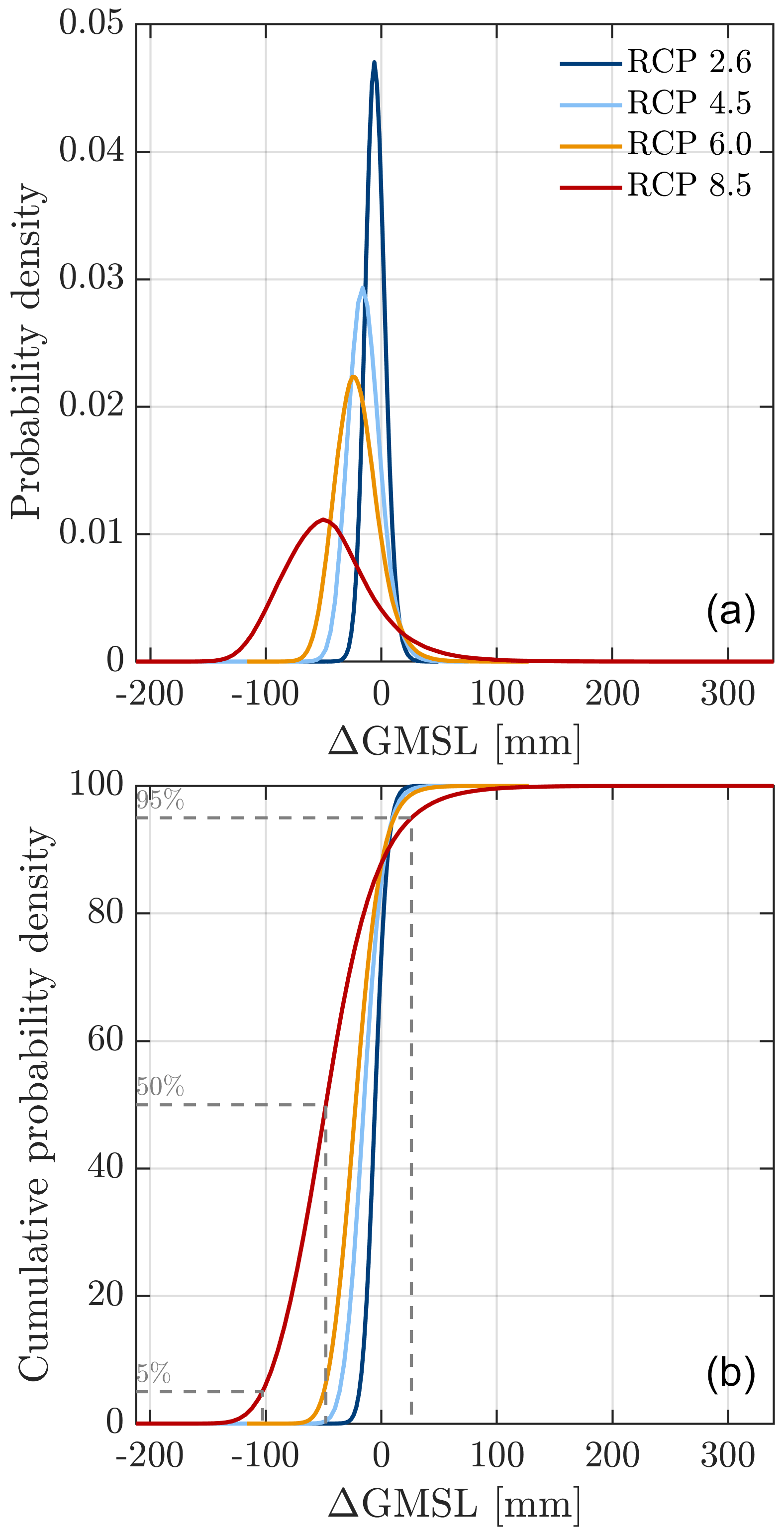
Figure 5 Probability density (a) and cumulative probability density (b) for projections of change in global mean sea level (ΔGMSL) in millimetres by the year 2300 under four RCP emissions scenarios. Dashed lines show the 5th, 50th, and 95th percentiles for the highest emission scenario RCP8.5.

4 Results

4.1 Projections of sea level rise from FR basin

We begin by presenting probabilistic projections of global mean sea level change from the Filchner–Ronne basin for four RCP scenarios. These projections were derived from surrogate models that were trained with our 500 member training ensemble of forward-in-time ice flow model simulations. We then evaluated these surrogate models with a 1 000 000 point sample (generated using Latin hypercube sampling) from our input parameter space to derive model responses, and calculated probability distributions using kernel density (Fig. 5).

Table 1 Contribution to global mean sea level (mm) at the years 2100, 2200, and 2300. The first number is the median projection, and values in brackets are 5 %–95 % confidence intervals

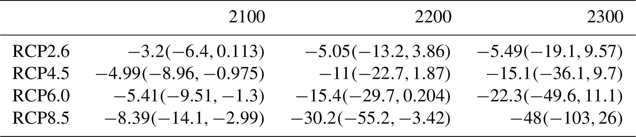
Our projections indicate it is most likely that the FR basin will undergo limited change or contribute negatively to global mean sea level by the year 2300. Under the lowest-warming scenario (RCP2.6: 0.77–1.7 ^∘C), ΔGMSL is limited, ranging between −19.1 mm (5th percentile) and 9.57 mm (95th percentile: Table 1). The probability distribution (Fig. 5) takes a near-to-normal shape, with a median projection close to zero (−5.49 mm), but it has a weak positive skew of 0.16 (calculated using the moment coefficient of skewness), with a tail extending towards a maximum sea level contribution of ∼ 50 mm. Projections of ΔGMSL under the medium-warming scenarios RCP4.5 and 6.0 range from −36.1 to 9.7 and −49.6 to 11.1 mm, respectively (Table 1). These distributions are more positively skewed than RCP2.6 (skewness coefficients of 0.29 and 0.39, respectively), with tails extending towards ∼ 100 mm of global sea level rise (Fig. 5). Extreme warming leads to the greatest uncertainty in projections, which range from −103 to 26 mm under RCP8.5 (Table 1). The median projection indicates a greater negative contribution to sea level rise under higher warming. However, the probability distribution is asymmetric, with a long tail (high positive skew = 0.77) that decreases exponentially away from the median and reaches a maximum ΔGMSL of 332 mm (Fig. 5). This long tail represents the potential for low-probability but high-magnitude contributions to sea level rise.

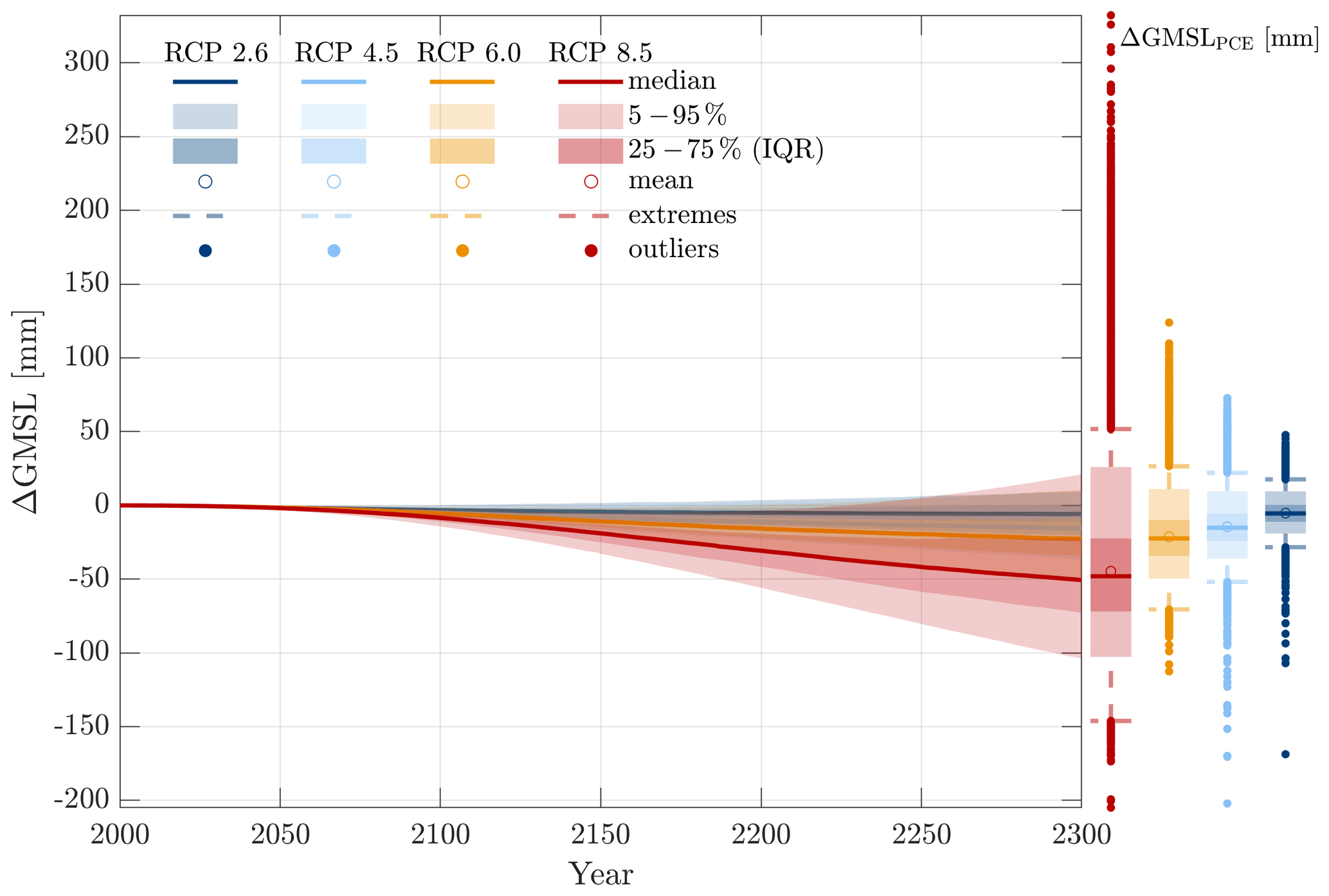
Figure 6 Projections of changes in global mean sea level (ΔGMSL) from 2000 and 2300 from our training ensemble of ice flow model simulations. Dark shading is the interquartile range (IQR) defined between the 25th and 75th percentiles. Lighter shading shows the 5th–95th percentiles. Box plots show the projections from the surrogate models (ΔGMSL_PCE) for each RCP scenario at 2300. Extreme values are located at 1.5 times the interquartile range away from the 25th and 75th percentiles. Values outside of these extreme bounds are considered to be outliers.

As our surrogate modelling is based around a single quantity of interest (ΔGMSL at the year 2300) it does not allow us to evaluate temporal changes in ice loss directly. Figure 6 instead presents projections through time from our 500-member training ensemble alongside the final ΔGMSL from each surrogate model (PCE). We also generate two additional surrogate models for each RCP scenario at the years 2100 and 2200 (Table 1) to evaluate projections at these time intervals, and we identify the temporal importance of parameters on projection uncertainty (see Sect. 4.2 and Fig. 7).

Both Table 1 and Fig. 6 show that the contribution to ΔGMSL and associated uncertainties increase through time. Within the next 100 years (up to 2100) we project little change in ice mass from the FR basin. This constitutes a small negative contribution to sea level rise of < 10 mm in all warming scenarios (Table 1), with a maximum range of −14.1 to 0.11 mm. By 2200 the spread of ΔGMSL has diverged based on warming scenario, with little change under limited forcing (RCP 2.6 = −5.05) and a greater negative contribution under higher warming (−30.2 in RCP8.5). Between 2200 and 2300 uncertainties increase dramatically in all warming scenarios, particularly in RCP8.5. Box plots in Fig. 6 show the projections generated from our surrogate model in 2300 alongside our ice flow model training ensemble. This shows that the probability distributions in the most likely range between 5 %–95 % generated from our surrogate models are largely similar to those found from our training ensemble in 2300. However, we note that the tails of these distributions, in particular for RCP8.5, extend substantially beyond the maximum ΔGMSL shown from our training ensemble alone (150 mm). While this is expected with more extensive sampling of our parameter space, we test the feasibility of ΔGMSL = 332 mm by taking the parameter values that led to this and re-evaluating the “true” ice flow model. This gives a slightly lower value of ΔGMSL = 250 mm but one that is still considerably higher than in our original training ensemble despite its relatively large size (N=500). This demonstrates the benefits of our surrogate modelling approach, as it was able to capture the possibility of more extreme sea level rise scenarios that were not exposed by the original sample. Recalculating the surrogate model for RCP8.5 including this “extreme” sample point reduces the maximum contribution to sea level rise to 288 mm.

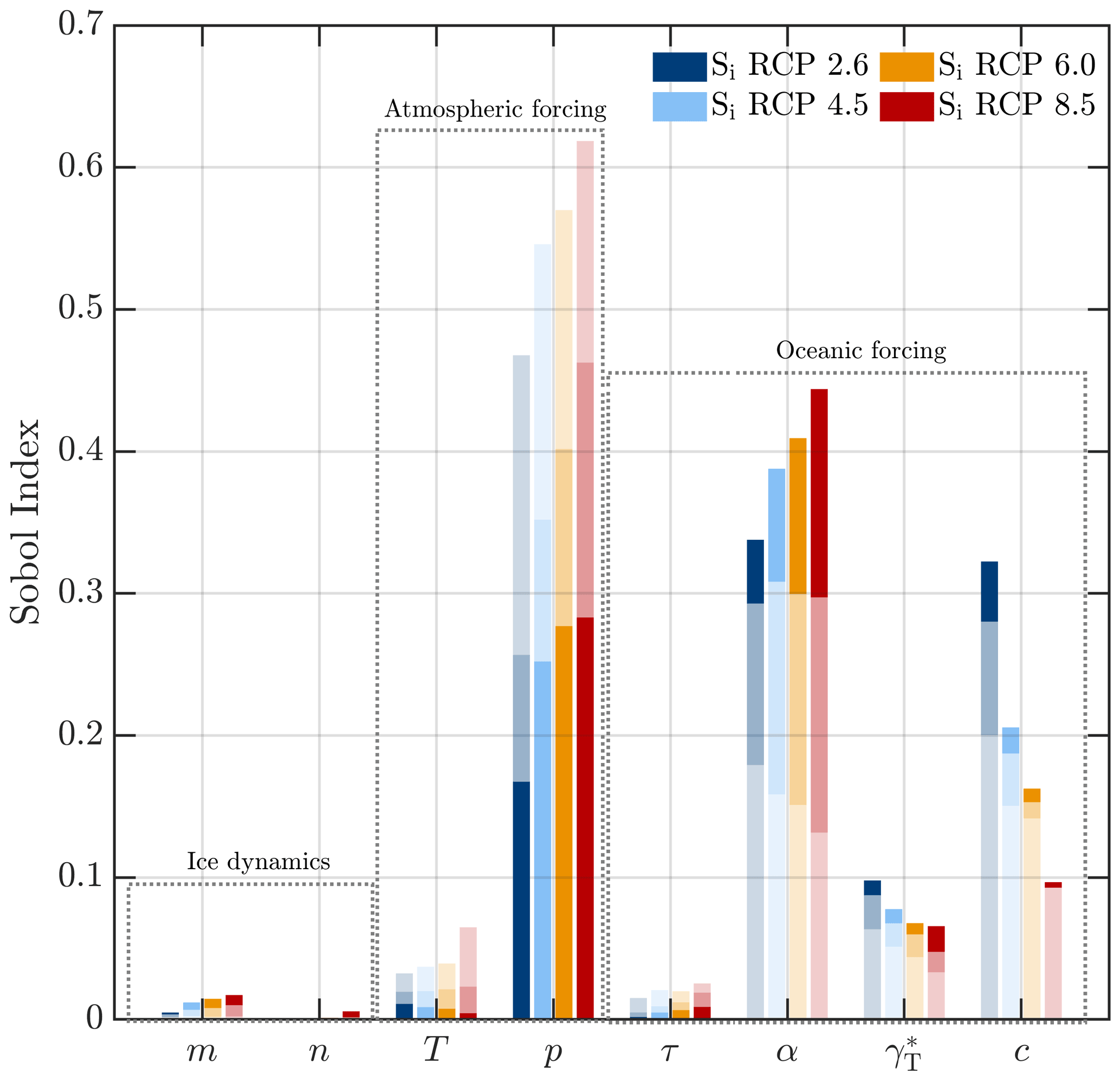
Figure 7 First-order Sobol indices, i.e. the fractional contribution of each input parameter on the uncertainty in our projections of ΔGMSL, for each RCP forcing scenario. Dark shading shows the Sobol indices for ΔGMSL in 2300. Two lighter shading colours represent Sobol indices at the years 2100 and 2200, to show the variability in parameter importance through time.

4.2 Parametric uncertainty

In this section we present the results of our sensitivity analysis, in which we determine how uncertainties in our input parameters (parametric uncertainty) impact our projections of ΔGMSL. To do this, first-order Sobol indices were decomposed from each of our PCE models (four RCP forcing scenarios) and for three time steps: 2100, 2200, and 2300, which are presented in Fig. 7. We additionally assessed the individual parameter-to-projection relationship, by re-evaluating our surrogate model for each parameter, while all other parameters were held at their sample point estimates (see Fig. S4).

By 2300 (dark shaded bars in Fig. 7) uncertainties in our four ocean forcing parameters collectively have the greatest fractional contribution to the uncertainty in our projections of global mean sea level contribution. This ranges from 60 % in RCP8.5 to 75 % for RCP2.6. Projection uncertainty in all RCP scenarios is primarily driven by ocean temperature forcing and the value of α used to scale atmospheric to ocean temperatures. Uncertainties attributed to α appear to increase both with warming scenario and through time. In all RCP scenarios, fractional uncertainty associated with α increases from 2100 to 2300 (light shaded bars in Fig. 7), coincident with an increase in the spread of ΔGMSL contribution (Fig. 6). In 2100, α has a greater impact on projection uncertainty in the lower-warming scenario. However, by 2300, the fractional uncertainty is greatest in RCP8.5, accounting for almost half of projection uncertainty (0.44) compared to 0.34 in RCP2.6. Re-evaluating the surrogate models varying only the value of α reveals a quadratic dependency of ΔGMSL on the value of the scaling coefficient (Fig. S4), which is consistent with the quadratic sensitivity of sub-shelf melt rates to ocean temperature forcing observed for the FR ice shelf cavity by Reese et al. (2018a). Under extreme warming (RCP8.5), this quadratic relation becomes stronger, and variability in α alone can cause ΔGMSL to range between −86 and 73 mm by 2300. Under all RCP warming scenarios the value of α contributes to a greater range of ΔGMSL than any other parameter (Fig. S4) and encompasses almost all of the 5 %–95 % spread of projections (Table 1).

Of our two ocean box model parameters, overturning strength (c) accounts for more projection uncertainty than the turbulent heat exchange coefficient (${\mathit{\gamma }}_T^{*}$) in all warming scenarios. This is consistent with the theory that sub-shelf melting at large and cold cavity ice shelves is predominantly driven by overturning strength (Reese et al., 2018a). The fractional importance of c has the greatest variability between forcing scenarios than any other parameter. Unlike α, uncertainty associated with c decreases with warming, from 0.32 in RCP2.6 to 0.1 for RCP8.5 (Fig. 7). The importance of the overturning strength, c, also increases with time, which is most pronounced in lower-warming scenarios, e.g. RCP2.6 where α and c are similar by 2300. This suggests that with greater ocean warming (in RCP8.5) and a transition to warm cavity conditions uncertainties in temperature (associated with the value of α) outweigh uncertainties in sub-shelf melt rates driven by the overturning strength alone. Conversely, in colder conditions (RCP2.6) variability in c has a greater control on heat supply for sub-shelf melt. A similar trend exists for uncertainties associated with ${\mathit{\gamma }}_T^{*}$: greater importance for lower-warming scenarios and increasing importance with time in all scenarios. However, in contrast to c, there is a greater relative increase in the Sobol index for the highest-warming scenario (RCP8.5) from 2100 to 2300; the importance of ${\mathit{\gamma }}_T^{*}$ doubled from 0.033 to 0.066 versus only a 54 % increase in RCP2.6. This suggests that as the FR ice shelf transitions to warm cavity conditions (∼ 2 ^∘C in RCP8.5) the heat exchange in the turbulent boundary layer may become a more important driver of sub-shelf melt than under colder conditions.

Atmospheric forcing parameters account for the second largest proportion of uncertainty in ΔGMSL by 2300. This is primarily driven by variability in the percentage increase in precipitation per degree of warming (p) and to a lesser extent the temperature scaling parameter (T). At all time intervals (2100, 2200, 2300), projection uncertainty attributed to p is largest based on warming scenario. Unlike α, Sobol indices for p decrease through time, which is asynchronous to increased uncertainty in ΔGMSL contribution (Fig. 6). In 2100, p accounts for over half of projection uncertainty in all scenarios (except RCP2.6), reaching a maximum of 0.62 in RCP8.5. p remains the dominant parameter in 2200 for higher-warming scenarios, but for RCP2.6 the Sobol index for p decreases to 0.26, less than both α and c. By 2300, the fractional importance of p is <0 3 and lower than α for all four warming scenarios. Evaluating the surrogate model (at the year 2300) for p only reveals a linear dependency on the value of p, where, as expected, increases in precipitation lead to a decrease in the contribution to GMSL, or in this case a greater negative contribution to GMSL (Fig. S4). In RCP8.5, p alone contributes between −8 and −80 mm of ΔGMSL (Fig. S4). This suggests that even with a limited (p = 4 %) increase in precipitation, and fixed melt rates, the FR basin is unlikely to contribute positively to ΔGMSL. However, in RCP2.6, increased accumulation with p<0.05 does not outweigh mass loss associated with sub-shelf melting and could lead to a small positive contribution to sea level rise.

Finally, uncertainties in our ice dynamical parameters relating to the non-linearity in the sliding (m) and flow (n) laws used in our model have a limited contribution to uncertainties in our projections of ΔGMSL (Fig. 7). The combined contribution of these parameters by 2300 under all warming scenarios (0.02 in RCP8.5) is an order of magnitude less than uncertainties associated with atmospheric and oceanic forcing (see Fig. S5 for Sobol indices for just m and n). Of the two parameters, m accounts for the most uncertainty in ΔGMSL, which is unsurprising given that basal sliding is likely to be the dominant component of surface velocities of the fast-flowing ice streams feeding the FR ice shelf. Despite low values of the Sobol indices, we note that uncertainties in both m and n increase with time and the strength of the temperature perturbation (Fig. S5). Increasing the values of m and n in isolation reduces the negative contribution to ΔGMSL, i.e. less mass gain (Fig. S4). In both cases, a stronger non-linearity in the ice flow (n), or more plastic like flow (m), allows for faster delivery of the ice to the grounding line in response to a perturbation.

Figure 8 Projected temperature changes and mass balance changes for RCP2.6 (a–d, blue lines) and RCP8.5 (e–h, red) between 2000 and 2300 from our training ensemble. Uncertainties are shown between 5 % and 95 % in light shading and between 33 % and 66 % in dark shading. (a, e) Global temperature anomalies. (b, f) Change in the rate of total mass change (M) in Gt yr⁻¹ calculated as P−D. (c, g) Change in the rate of accumulation (P) with respect to our control runs (P_rcp−P_ctrl), integrated over the grounded area in Gt yr−1. (d, h) Change in the rate of ice discharge (D) calculated with respect to our control runs (D_rcp−D_ctrl), integrated across the grounding line in Gt yr⁻¹.

4.3 Partitioned mass change

Our Sobol indices reveal that the percentage change in precipitation and ocean temperature scaling are the main drivers of uncertainty in changes in global mean sea level. To further examine the relative importance of precipitation and sub-shelf melt parameters on mass change in the FR basin, we take our training ensemble and partition components of mass balance (accumulation and discharge) using the input–output method. We calculated the integrated input accumulation (P) across the grounded area and the total integrated discharge (D) output across the grounding line with respect to our control runs. These mass balance components, as well as total mass change ($M=P-D$), are shown for the low-warming (RCP2.6) and high-warming (RCP8.5) scenarios in Fig. 8) and for intermediary scenarios in Fig. S6.

Mass change under the lowest-warming scenario (RCP2.6) closely follows the temperature anomaly trend and appears primarily driven by increases (and subsequent decreases) in accumulation with warming. In the first 50 years, mass balance increases to 12.6 (6.56–18.6) Gt yr⁻¹ (where values in brackets here and in the remainder of this section are 5 %–95 %). This is primarily due to an increase in accumulation at a rate of 15.2 Gt yr⁻¹ in 2050, which is offset by a limited increase in discharge across the grounding line (2.5 Gt yr⁻¹) during this period. Between 2050 and 2100 accumulation remains constant and discharge increases, which consequently reduces the rate of total mass gain. Uncertainties associated with accumulation are greater than those for discharge during this period (Fig. 8c), which is consistent with the high contribution of the percentage increase in precipitation to projection uncertainty in 2100 (Fig. 7). The rate of mass gain continues to decrease after 2100, alongside a reduction in the temperature perturbation in RCP2.6 and decelerating accumulation. During this period, discharge across the grounding line stabilizes at a median of 10 Gt yr⁻¹, but the uncertainty range increases dramatically to −8 to 26 Gt yr⁻¹, which coincides with an increasing importance of parameters relating to sub-shelf melt from 2200 to 2300 (Fig. 7). By 2300 this drives the mass balance towards zero, at which accumulation is approximately balanced by ice discharge.

Under RCP8.5 forcing the spread of mass change in 2300 is driven by anomalies in ice discharge. During the first 150 years, surface accumulation steadily increases at an average rate of 50 Gt yr⁻¹, which is consistent with increased temperature forcing of 6.4 ^∘C. During this period, increases in discharge lag that of accumulation, averaging only 9.6 Gt yr⁻¹, which can partly be explained by the prescribed time delay between atmospheric and oceanic warming (τ: Eq. 14). Hence, it appears likely that total mass balance will remain positive up to 2150, as no parameter combinations (training ensemble members) are able to sufficiently increase ice discharge above that of accumulation. Consistent with other forcing scenarios, uncertainties in accumulation are also greater than those associated with discharge, which corresponds to greater projection uncertainty attributed to p up to 2200 (Fig. 7).

After 2150, the rate of temperature increase is reduced, which leads to a reduction in surface accumulation that plateaus at ∼ 140 (86–202) Gt yr⁻¹ between 2200 and 2300. Despite a limited change in temperature (+1.6 ^∘C) between 2150 and 2300 (relative to 2000 to 2150), discharge continues to increase linearly from 31 to 92 Gt yr⁻¹. Simultaneously, uncertainties in discharge increase substantially and span 0.05–0.76 mm yr⁻¹ (5–95th percentiles) of sea level equivalent volume in 2300. This suggests that the atmospheric temperature anomaly itself becomes less important than the amount by which atmospheric temperatures are scaled to ocean warming, i.e. the value of α, where variability in α alone accounts for most of the range of sea level contribution (Fig. 7 and Fig. S4). Indeed, the spread of total mass change (M) closely follows the uncertainties in ice discharge, where it is possible, albeit unlikely, that certain combinations of parameters (within the 5–95th percentiles) allow for mass imbalance (P<D) and a positive contribution to sea level.

Variability in ice discharge alone also reveals the spread of potential positive contribution to sea level rise that would have occurred in our simulations if surface accumulation had remained unchanged. To explore this, we rerun our median simulation under RCP8.5 forcing using the same parameter values, but we keep surface mass balance fixed at its initial value. This reveals that increases in sub-shelf melt alone would contribute 84 mm of global mean sea level rise (as opposed to −50 mm), and highlights the important and compensating effect accumulation has on the sign of our sea level projections.

Figure 9 Changes in grounded area and grounding line position for RCP8.5. Panel (a) shows change in grounded area (ΔGA calculated as GA_rcp − GA_ctrl) in ×10⁴ km². Coloured lines represent the 5th, 50th, and 95th percentiles of the projections of ΔGMSL rather than the percentiles of the change in grounded area itself. However, they are generally close to the grounded area results. Panel (b) shows the FR basin and bed elevation in metres above (green to brown) and below (light to dark blue) sea level. Coloured lines show grounding line positions from our training ensemble that lie closest to our percentiles (5 %, 50 %, and 95 %) from our surrogate model projections, with respect to control runs (dashed grey lines). Two additional grounding line positions are shown; the maximum ΔGMSL from our training ensemble (orange) and the maximum ΔGMSL from our surrogate model (magenta), which we evaluated separately to our initial training ensemble of simulations.

4.4 Grounded ice loss

In this section we explore the changes in grounded area throughout our simulations to see how our projections of mass change correspond to the retreat of the grounding line. Figure 9 presents changes in grounded area with respect to the control runs (Fig. 9a) and grounding line positions from members of our training ensemble closest to our 5 %, 50 %, and 95 % percentile projections of ΔGMSL from our surrogate models (Fig. 9b) for RCP8.5, while additional RCP scenarios are shown in Figs. S7–S9.

Despite the negative contribution to ΔGMSL likely under all warming scenarios (50th percentiles: Table 1), our results show that these median projections correspond to simulations that all experience a reduction in grounded area by 2300 (Fig. 9 and Figs. S7–S9). In all scenarios there is limited grounding line retreat in the next 100 years (up to 2100), amounting to only −716 km² (−4800 to 2050 km²: 5 %–95 %) change in grounded area in RCP8.5. After 2150, grounded area decreases more rapidly, and the spread of change in grounded area increases within each forcing scenario. This coincides with the timing of a reduction in the rate of accumulation and increases in the rate of grounded ice discharge (Fig. 8). This is particularly the case in RCP8.5 (Fig. 9), where more substantial ungrounding coincides with a sharp increase in uncertainty in ice discharge in 2200 and the increasing importance of sub-shelf parameters on projection uncertainty (Fig. 7). This indicates that parameters controlling melt rates are responsible for the spread of grounded ice loss via variations in sub-shelf melt applied close to the grounding line. Ultimately this drives the long positive tail of projections of sea level rise contribution (ΔGMSL: Fig. 5).

While median projections for all RCP scenarios experience a loss of grounded area by 2300, in the lower-warming scenarios (RCP2.6 and RCP4.5) this is relatively limited (< 800 km²), with the exception of some retreat of the Möller and Institute ice streams (Figs. S7–S9). This suggests that these ice streams are prone to some ungrounding even with limited increases in sub-shelf melting. The likelihood of retreat and complete collapse of these ice streams increases dramatically with warming (RCP6.0 and 8.5). In RCP8.5 perturbations become large enough for possible (but less likely) retreat of additional regions, in particular the Rutford and Evans ice streams draining into the western part of the Ronne Ice Shelf and some retreat of ice streams feeding the Filchner Ice Shelf (Fig. 9). Our separate additional simulation that validated the upper end of sea level projections from our surrogate model (ΔGMSL = 250 mm) shows that there is potential within our parameter space (beyond our initial ensemble) for the grounding line to retreat much further inland (Fig. 9). This is characterized by runaway retreat of Möller and Institute ice streams, likely due to being topographically unconfined and rested upon a retrograde bed below sea level (Fig. 9). This suggests that increases in sub-shelf melt with climate warming have the potential to reduce ice shelf buttressing and force substantial grounded ice loss.

5 Discussion

Here, we have used an uncertainty quantification approach to assess the spread of future changes in global mean sea level (ΔGMSL) contribution from the Filchner–Ronne region of Antarctica under different RCP emissions scenarios. We have taken a large and extensive sample of parameter space using a novel surrogate modelling approach, and our results show it is highly likely that, within the bounds of our input parameter space, ΔGMSL from the FR basin will be negative. Under RCP2.6 forcing, during which atmospheric temperatures increase by 2 ^∘C (Fig. 4: in line with the targets of the Paris agreement), this region is likely to remain close to balance (accumulation ≈ discharge) and contribute to −19.1 to 9.57 mm (5 %–95 %) of sea level rise by 2300. Under higher-warming scenarios, projections of sea level rise become increasingly negative, but the uncertainties in these projections also increase dramatically. In the highest-warming scenario (RCP8.5), the FR basin could contribute anywhere between −103 and 26 mm (5 %–95 %) to global mean sea level. Our projections are predominantly negative due the mitigating effect of increased accumulation with warming on sub-shelf-melt-driven increases in ice discharge.

Increases in precipitation across the Antarctic Ice Sheet are known to have an important mitigating effect on the contribution to global sea level rise (Medley and Thomas, 2019; Winkelmann et al., 2012). Unlike other parts of West Antarctica, the Weddell Sea showed a strong accumulation trend during the 20th century (Medley and Thomas, 2019) and limited change in dynamic ice discharge towards the end of the century (Rignot et al., 2019). Our simulations show that continued increases in accumulation during the 21st century, driven by warming, can outweigh slow increases in ice discharge associated with sub-shelf melting (Fig. 8). This may be enough to stabilize some of the major ice streams, in particular Institute and Möller (see 50 % line in Fig. 9). In most cases, mass gain continues through to 2300, despite increases in the rate of ice discharge and slowdown in the accumulation trend, both of which are not enough to switch to mass loss/positive ΔGMSL by 2300. We continued our median RCP8.5 simulation for a further 200 years with forcing held at 2300, and we found that total mass balance (accumulation − discharge) remained positive (mass gain) by 2500. These findings are consistent with previous regional modelling studies which showed that when applying either both accumulation and sub-shelf melt anomalies through time (Wright et al., 2014; Cornford et al., 2015) or a step function in accumulation alongside sub-shelf melting (Schlegel et al., 2018) it is possible for accumulation to suppress the effects of increased sub-shelf melt. This is in contrast to Antarctic-wide simulations that do not impose changes in surface accumulation through time (Ritz et al., 2015; Levermann et al., 2020) and hence project greater ice loss and sea level rise contribution from this region. Overall, our results demonstrate that the FR basin is particularly sensitive to future accumulation changes, which are capable of stabilizing this region in response to climate warming.

Despite the important role that precipitation plays in suppressing ice loss from the FR basin, our sensitivity analysis reveals that the percentage increase in precipitation per degree of warming p is the second largest contributor (approx. 30 % in RCP8.5) to uncertainties in our projections. Hence, we can identify the representation of accumulation changes with warming in ice sheet models as a target area for further research, in order to better constrain projections of sea level contribution. However, modelling future precipitation trends is challenging and CMIP5 models themselves show large temporal and spatial variability in projected precipitation trends with warming (Tang et al., 2018; Palerme et al., 2017; Rodehacke et al., 2020). Despite this, it has been assumed that there is a general correlation between precipitation and temperature anomalies. As a result, temperature scaling of precipitation (as used in this study) is a common approach in ice sheet modelling, most of which uses a Clausius–Clapeyron relation, equivalent to a 5 % spatially uniform increase in precipitation (Golledge et al., 2015; Gregory and Huybrechts, 2006; Garbe et al., 2020; DeConto and Pollard, 2016). But, as we have shown here, small variations in p can have a large effect on the spread of ΔGMSL projections, and better constraints on the value of p are needed.

Sampling from an uncertainty distribution for p has been valuable to capture the spread of future accumulation change predicted in a warming climate; however, one caveat to this is the use of uniform priors. In the absence of additional constraints, we cannot make a more informed choice on the uncertainty distribution of p, but it is possible that this leads to a greater spread, or skewed distribution of accumulation changes, with respect to those predicted by CMIP GCMs. Validating these parameterizations to climate model predictions should be the focus of future work. Recent work by Rodehacke et al. (2020) has made improvements towards Antarctic estimates for p and found that the assumed correlation/or lack thereof between temperature and precipitation anomalies has strong regional differences, which may invalidate the use of a spatially invariant value for p. Instead they propose spatially variable values of p across the Antarctic Ice Sheet. Over the FRIS, they showed p = 4 %–6 %, which is consistent with values used in this study, but may reach up to 10 % in inland regions of the FR basin (Rodehacke et al., 2020). Thus, using a spatially invariant value for p may lead to under- or overestimates of precipitation across the catchment. This is even more important when conducting Antarctic-wide simulations, and future studies should move towards using a spatially variable value for p, or ultimately conduct coupled atmosphere–ocean–ice sheet simulations.

Our probabilistic projections have shown that a negative ΔGMSL is most likely from the FR basin. Nonetheless, uncertainties associated with our input parameters reveal that it is also possible within our parameter space for the FR basin to contribute positively to sea level rise. This occurs predominantly under RCP8.5 forcing, where the long tail of the projections in Fig. 5 reflects these more “extreme” (maximum of 332 mm by 2300) yet unlikely contributions to ΔGMSL. Hence, it is possible for sub-shelf melt to increase enough to outweigh 21st century accumulation, by forcing substantial increases in ice discharge (Fig. 8) and un-grounding of the ice streams feeding the FRIS (Fig. 9). These high-magnitude contributions to sea level rise are characterized by the rapid retreat of the lightly grounded Möller and Institute ice streams, which, once initiated, continues unabated across the Robin subglacial basin throughout our simulations (maximum GMSL simulation: Fig. 9). Additional retreat occurs predominantly in the ice streams feeding the Ronne ice shelf (Evans and Rutford ice streams and Carlson Inlet), suggesting that these regions are likely to be the dominant contributors to future sea level rise. There is also some potential for un-grounding in the ice streams feeding the Filchner ice shelf, but this is less than elsewhere in the region (Fig. 9). Retreat of the grounding line in our simulations is consistent with the magnitude and spatial pattern of retreat simulated in other studies in response to increased ocean-driven melt rates, with comparable projections of sea level rise contribution (approx 150–160 mm) to the high end of our results (up to 300 mm) (Schlegel et al., 2018; Wright et al., 2014; Cornford et al., 2015).

Greater variability in ice discharge from the 22nd century onwards (Fig. 8) coincides with an increase in the spread of our projections, suggesting that sub-shelf melt could strongly influence the region's potential contribution to sea level rise. Indeed, our sensitivity analysis clearly reveals that ocean forcing parameters are the dominant component of uncertainties in our projections of sea level contribution from the FR basin (Fig. 7). This sensitivity corroborates the well-established theory that ocean forcing and the impact it has on sub-shelf melt rates are a dominant, yet uncertain, driver of Antarctic Ice Sheet mass loss (Seroussi et al., 2019, 2020; Cornford et al., 2015; Bulthuis et al., 2019). Of our ocean forcing parameters, the magnitude by which global atmospheric temperature anomalies are scaled to ocean temperature changes α appears highly uncertain, amounting to 44 % of projection uncertainty in RCP8.5 (Fig. 7). This is consistent with the high sensitivity to the value of α across the entire Antarctic Ice Sheet (Bulthuis et al., 2019). Going forward, given the impact of a linear scaling and the value of α on projection uncertainty, it may be more suitable to instead force ocean temperature changes with the results of CMIP ocean models directly (e.g. the approach used in ISMIP6 proposed by Jourdain et al., 2020). In addition to uncertainties in ocean temperature forcing, it remains challenging to accurately represent ice shelf melt rates, and their sensitivity to temperature changes, in ice sheet models. While melt parameterizations such as the PICO box model (Reese et al., 2018a) are a substantial advancement in our ability to efficiently apply sub-shelf melting in a physically plausible way, they remain a simplification of observed melt rate patterns, and those simulated by ocean models. Hence, it is possible we do not capture the same spatial distribution or magnitude of melt in highly buttressed regions of the ice shelf as shown in observations, which could ultimately impact the (in)stability of the grounding line.

Alongside the mitigating effect of accumulation, using a linear scaling of ocean temperatures, and a simple melt parameterization, may both be responsible for our simulations not projecting a substantial increase in sub-shelf melt or contribution to global mean sea level rise. Crucially, it appears that we are not capturing the regime shift from “cold” to “warm” cavity conditions as seen in ocean model results (Hellmer et al., 2012, 2017; Hazel and Stewart, 2020). Simulations by Hellmer et al. (2012) showed relatively warm ocean waters could flush the ice shelf cavity and increase the area-integrated (fixed ice shelf extent) basal mass loss from 80 to 1600 Gt yr⁻¹ by the year 2100. By comparison, basal mass loss during our RCP8.5 training ensemble of simulations (integrated over the initial ice shelf area) reached a maximum of only 1200 Gt yr⁻¹ some 200 years later (2300). Beyond our training ensemble of 500 simulations, we may start to capture the same magnitude of basal mass loss, which is reflected in the long tail of positive contribution to sea level rise in RCP8.5 projections. However, the key difference is that melt rates increase at a slow and steady rate over the 150-year period and do not impose a rapid switch from cold to warm conditions which may be possible with a sudden flushing of warm water into the ice shelf cavity. Additionally, our Bayesian-analysis-derived probability distributions for ocean forcing parameters, while potentially generating more realistic melt rates, may have reduced the probability of sampling high-melt-rate distributions sufficient to impose a regime shift that may have occurred with wider sampling. To fully capture such a regime shift, and the effects this would have on ice shelf thinning, loss of buttressing, and increases in ice sheet discharge, it is necessary to run fully coupled ice–ocean model simulations. Recent work performing coupled simulations in the FR region (Naughten et al., 2021) found that ice shelf melt rates are unlikely to increase over the next century, and thus the region will have a limited contribution to sea level rise until ocean temperatures increase substantially (+7 ^∘C). While more coupled modelling studies emerge, they are currently only computationally feasible for regional configurations and have yet to be accomplished on an ice sheet scale. In the meantime, melt parameterizations will remain important for future ice sheet simulations, and so work should still focus on improving their ability to capture the physical behaviour of ocean models, as well as the choice of ocean temperature forcing used to perturb those melt rates.

In contrast to atmospheric and oceanic forcing parameters, those related to ice flow dynamics in our model appear to play a less important role in uncertainties in projections of ΔGMSL. Consistent with other studies (Ritz et al., 2015; Bulthuis et al., 2019; Gillet-Chaulet et al., 2011; Alevropoulos-Borrill et al., 2020), we have shown that stronger non-linearity in our basal sliding and ice flow laws (increasing values of m and n) reduces the response time to a temperature perturbation, allowing for faster delivery of ice to the grounding line and a greater contribution to sea level rise. By varying the value of m in the Weertman sliding law, we have captured a large range of amounts of basal sliding, and this has been fully integrated into our uncertainty analysis. However, this may not have captured the full spread of basal sliding possible under different sliding laws and/or spatially variable fields of m. Different sliding laws (e.g. Budd sliding) may allow for even faster delivery of ice to the grounding line and thus greater contributions to sea level rise (Schlegel et al., 2018; Brondex et al., 2019). We are also not accounting for any transient variability in our basal slipperiness and ice rheology fields, which is not yet captured in most ice flow models but may additionally increase sea level rise. Progress is being made towards assessing the sensitivity of sea level projections to the choice of sliding law (Brondex et al., 2017, 2019; Cornford et al., 2020). Future work will benefit from choosing the form of the sliding law (Ritz et al., 2015; Gillet-Chaulet et al., 2016) and/or determining spatially variable values for m (De Rydt et al., 2021; Joughin et al., 2010) that best replicate regional observations of ice loss. This will help to constrain uncertainties associated with the prescription of basal sliding, but this remains an active area of research.

The surrogate modelling approach used in this study has been a powerful tool for exploring the future behaviour of the FR basin of Antarctica. We have shown that by extensively sampling the parameter space and efficiently propagating this through our surrogate models, we get a greater spread of results, and thus insights into the future of the region, than we would have from our already large ensemble. Overall, our results have shown that regional increases in accumulation assumed with warming are likely to have an important stabilizing effect on the ice loss from the FR basin under scenarios of future climate change. There is still some potential for a positive contribution to global mean sea level rise under high-sub-shelf-melt scenarios. This means that the sign of ΔGMSL projections from the FR basin cannot be fully constrained. Parameters driving both accumulation and sub-shelf melting are highly uncertain, and we identify them as priority areas for research, where more accurate parameterizations will help to constrain future projections, not only from the FR basin but also the entire Antarctic Ice Sheet. Future coupled atmospheric–ocean–ice sheet simulations will help to more accurately capture feedbacks between the atmosphere and ocean on the evolution of the ice sheet, but remain computationally challenging on a pan-Antarctic scale. In addition to coupled simulations, it is important to consider a number of additional processes that have not been captured in our ice flow model simulations. These include iceberg calving and the retreat of the ice front; evolution of damage of the ice shelf, which is becoming of emerging interest in the ice sheet modelling community; and the potential for hydrofracture-driven ice shelf collapse under increased surface melt. All of these processes remain highly uncertain, largely due to the challenges of implementation in ice sheet models, but equally have important implications for ice loss and the contribution to global sea level rise, and future work to incorporate these into similar studies is necessary. Future studies would also benefit from calibrating ice sheet models with observations in order to reduce uncertainties and constrain future projections by narrowing the parameter space for future simulations based on their fit to observations (Wernecke et al., 2020; Ritz et al., 2015; DeConto and Pollard, 2016; Reese et al., 2020) . As the number and time span of observations increases, we will be able to better initialize our ice sheet models to present-day conditions prior to future simulations. Overall, employing uncertainty quantification techniques in future studies will help to provide more robust estimates of potential sea level rise and identify priority areas for better constraining these projections.

6 Conclusions

This study set out to implement an uncertainty quantification framework (UQLAB) for use alongside the ice flow model Úa and use this to quantify uncertainties in projections of mass loss from the Filchner–Ronne region of Antarctica. We used a novel surrogate modelling approach to extensively sample an input parameter space to determine the forward propagation of uncertainties. Our probabilistic projections indicate that this region may not undergo dramatic ice loss under climate warming scenarios and instead have a negative contribution to global mean sea level rise. This is primarily due to the effects of increased accumulation assumed with greater moisture content in a warmer climate that is capable of suppressing mass loss attributed to ocean-driven increases in sub-shelf melt rates. Despite this, we find that there is the potential, albeit highly unlikely, within the bounds of our input parameter space, for a substantial positive contribution to global mean sea level. In these high-mass-loss scenarios, sub-shelf melting increases enough to outweigh accumulation and force major retreat of some of the ice streams flowing into the FRIS. Uncertainties associated with parameters driving accumulation and sub-shelf melt account for most of the spread of future changes in global mean sea level, and we highlight these as priority areas for constraining projections of ice loss. Future work would benefit from employing uncertainty quantification techniques similar to those used in this study, to fully assess the spread of future projections of sea level rise, not only from the FR basin but also across the entire ice sheet.

Appendix A: Model inversion for basal slipperiness C and ice rheology A parameters

To estimate the rate factor (A) and basal slipperiness coefficient (C) for each of our randomly sampled combinations of m and n, we use the inverse capabilities of Úa to minimize the misfit between observed (u_obs) and modelled (u_mod) velocities. Observed velocities are MEaSUREs InSAR-based Antarctica ice velocities (Version 2) from 1996 to 2016 and with a spatial resolution of 450 m (Rignot et al., 2011; Mouginot et al., 2012). Ice velocities were linearly interpolated onto our model mesh. Úa uses a standard inverse methodology in which a cost function J, which is the sum of a misfit (I) and regularization (R) term, is minimized. The gradients of J with respect to A and C are determined in a computationally efficient way using the adjoint method and Tikhonov-type regularization. The misfit (I) and regularization (R) terms are defined as

$$\begin{array}{}\text{(A1)}& {\displaystyle }I={\displaystyle \frac{\mathrm{1}}{\mathrm{2}\mathcal{A}}}\int {\left(u_{\text{mod}}-u_{\text{obs}}\right)}^{\mathrm{2}}/{\mathit{ϵ}}_{\text{obs}}^{\mathrm{2}}\mathrm{d}\mathcal{A},\text{(A2)}& {\displaystyle }R={\displaystyle \frac{\mathrm{1}}{\mathrm{2}\mathcal{A}}}\int \left({\mathit{\gamma }}_{\mathrm{s}}^{\mathrm{2}}{\left(\mathrm{\nabla }{\log }_{\mathrm{10}}(p/\widehat{p})\right)}^{\mathrm{2}}+{\mathit{\gamma }}_{\mathrm{a}}^{\mathrm{2}}{\left(\mathrm{\nabla }{\log }_{\mathrm{10}}(p/\widehat{p})\right)}^{\mathrm{2}}\right)\mathrm{d}\mathcal{A},\end{array}$$

where $\mathcal{A}=\int \mathrm{d}\mathcal{A}$ is the area of the model domain, ϵ_obs represents measurement errors, and $\widehat{p}$ represents the a prior values for model parameters ($\widehat{A}$ and $\widehat{C}$). Tikhonov regularization parameters γ_s and γ_a control the slope and amplitude of the gradients in A and C. Optimum values were determined using L-curve analysis and are equal to γ_s=10000 and γ_a=1 for all results presented. The inversions are run for the number of iterations needed for the cost function to converge. The number of iterations needed can vary depending on the values of m and n. Instead of using a fixed number of iterations, each inversion was terminated when the norm of the function gradient $\left|\mathrm{\nabla }f\right(x\left)\right|$ becomes sufficiently small. We tested several values for $\left|\mathrm{\nabla }f\right(x\left)\right|$ and found 10⁻⁴ was sufficient and that values any smaller did not substantially improve the cost function or substantially affect the transient behaviour in a forward-in-time model run.

Prior to our uncertainty quantification routine (see Sect. 3.5) we generated a 75-member “library” of inversions for every half integer between 2 and 9 for m and between 2 and 4 for n. For these 75 inversions we defined prior values as follows: $\widehat{A}=\mathit{ϵ}/{\mathit{\tau }}^n$ with ϵ = 10⁻⁴ yr⁻¹ and τ_e = 80 kPa, which for n=3 gives $\widehat{A}\approx$ 2 × 10⁻⁹ ${\mathrm{kPa}}^{-\mathrm{3}}{\mathrm{yr}}^{-\mathrm{1}}$ equivalent to an ice temperature of approx. −25 ^∘C using an Arrhenius temperature relation (Cuffey and Paterson, 2010). $\widehat{C}=u_b/{\mathit{\tau }}_b^m$ with u_b = 10 m yr⁻¹ and τ_b = 80 kPa. This library of inversions was designed to make it computationally feasible to incorporate a model inversion before every forward model run into our uncertainty analysis. For each of our randomly sampled values of m and n, we select the closest inversion from our library as the a priori values for A and C. These priors provide a good initial estimate of the spatial fields of A and C, which means the subsequent inversions need far fewer iterations to converge. After each inversion we advected C beneath the ice shelf to avoid a sharp gradient in C downstream of the grounding line in the case of glacier advance. We note that the model-calculated velocities for each model inversion will vary slightly based on the value of m and n used and the resultant fields of A and C. However, we find all training ensemble members (N=500) to provide an optimal fit to observations and that the misfit between observed and modelled velocities varies by only 1 m yr⁻¹, which is small with respect to measurement errors.

Appendix B: Bayesian optimization of ocean box model parameters

The majority of our parameters (Fig. 3) are reasonably well constrained; i.e. there is good a priori information on their probable distributions. However, some parameters used to force future simulations of sea level rise from Antarctica are less well known, which could lead to wide and potentially unrealistic estimates of future sea level rise. When prior information on parameter values is poor, it is best to take a non-parametric approach, in which the probability distributions are constructed based on observations. This can be done using Bayes' theorem:

$$\begin{array}{}\text{(B1)}& \mathit{\pi }\left(\mathit{\theta }\right|Y)=\mathrm{\ell }(\mathit{\theta };Y\left)\mathit{\pi }\right(\mathit{\theta }),\end{array}$$

where the posterior probability distribution of θ (a hyperparameter) given Y observations is equal to the likelihood (ℓ) of θ given Y multiplied by the prior probability distribution π(θ). We conduct this analysis on the four “hyperparameters” used in the box model. These are the time delay (τ) and scaling coefficient (α) used to force changes in ocean temperature through time (Eq. 14) and two physical parameters that additionally control sub-shelf melt: the turbulent heat exchange coefficient ${\mathit{\gamma }}_T^{*}$ and the strength of the overturning circulation c (see Reese et al., 2018a; Olbers and Hellmer, 2010). While some information exists on all these parameters, their bounds and distributions are not well known. The primary aim is not to find single point estimates for these parameters but to obtain an optimal range of parameter values that fit model-predicted melt rates to observations. These posterior distributions are then used as input to our uncertainty analysis (see Fig. 3). We conduct this Bayesian optimization using the tools in UQLab, including specifying a prior input model, surrogate models, and the Bayesian inversion itself (Marelli and Sudret, 2014).

B1 Priors

Prior probability distributions of our four parameters take into account any available information on their values before our Bayesian calculation. For the scaling coefficient (α) and time delay τ we used the values presented in Levermann et al. (2020) (see outline in Section 3.4) as the a priori information on the probability distributions of these parameters (Fig. B1). While some ranges for the heat exchange coefficient (${\mathit{\gamma }}_T^{*}$) and overturning strength (c) have been proposed (Reese et al., 2018a; Olbers and Hellmer, 2010), their probability distributions are unknown. Therefore, we use non-informative priors; i.e. we do not prescribe any prior information about these parameters and use a uniform distribution within the bounds $c\in [\mathrm{0.1},\mathrm{9}]$ Sv m³ kg⁻¹ and ${\mathit{\gamma }}_T^{*}\in [\mathrm{5}\times {\mathrm{10}}^{-\mathrm{6}},\mathrm{1}\times {\mathrm{10}}^{-\mathrm{4}}]$ m s⁻¹ given by Reese et al. (2018a) Olbers and Hellmer (2010) (see Fig. B1). However, we do know that these parameters are related, and certain combinations mean that the physics in the box model no longer hold Reese et al. (2018a). To specify the dependence between values of ${\mathit{\gamma }}_T^{*}$ and c and ensure that values outside of these bounds are not sampled, we prescribe a Gaussian copula with a correlation of p=0.9. To test the sensitivity of our posterior distributions to our specification of the priors, we repeated the analysis for several prior distributions, with or without copulas, and found our results were largely insensitive to our priors (Fig. B1).

B2 Surrogate modelling

Rather than use a single area-integrated value of sub-shelf melt, and to preserve some of the spatial distribution of melt rates across the shelf, we chose to tune our parameters to observations, using average melt rates within each melt box. As Bayesian analysis requires a large number of iterations to settle on a posterior distribution, we first construct five surrogate models to emulate calculated melt rates in each ocean box. For this we use the same method as our surrogate modelling for changes in global mean sea level (see Sect. 2). We sample 2000 points from our prior probability distributions using Latin hypercube sampling and use these to directly evaluate sub-shelf melt rates in the box model. Each simulation is run in a diagnostic mode for our nominal start year of 2000, using observations of topography. We assessed the performance of our surrogate models by taking a separate validation sample from the parameter space, and we found a good fit between true and surrogate modelled melt rates (Fig. S10).

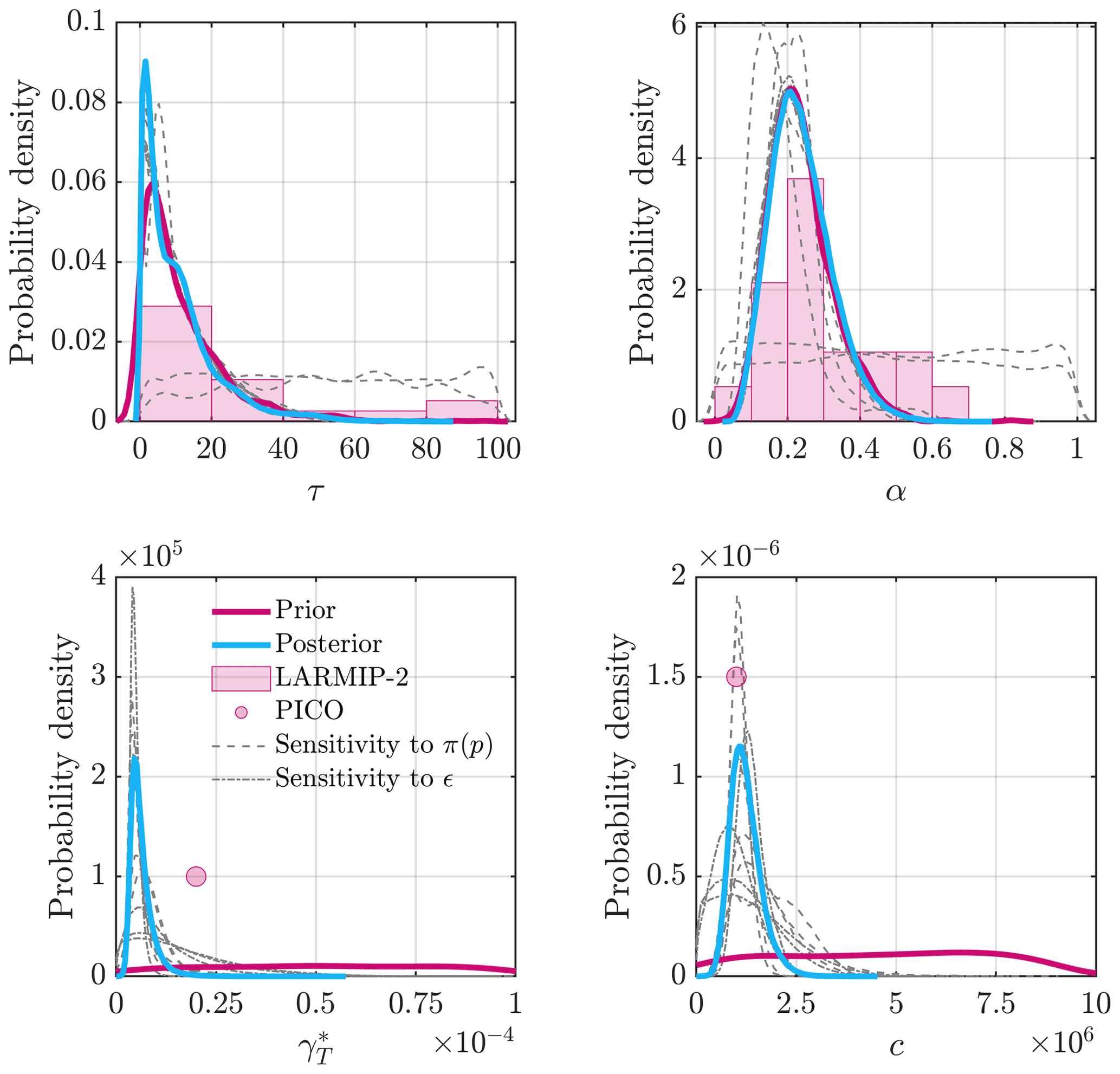
Figure B1 Results from our Bayesian analysis. Solid pink line shows priors using uniform bounds for ${\mathit{\gamma }}_T^{*}$ and c and prior knowledge from the LARMIP-2 distributions for τ and α (pink bars). Solid blue lines show the resultant posterior distributions using the pink lined priors. We performed a number of additional sensitivity experiments in which we varied either the prior distributions (dashed grey line) or the likelihood function (solid grey line). The lines shown are the resultant posterior distributions. These show that our results are largely insensitive to our choice of priors (except in the case of uniform priors for τ and α, which given the information we have are unsuitable) or the likelihood function used. Pink circles show the values proposed for ${\mathit{\gamma }}_T^{*}$ and c by Reese et al. (2018a) for circum-Antarctic simulations using the PICO box model. Point estimates from our posterior probability distributions show our c value is close, while values of ${\mathit{\gamma }}_T^{*}$ appear likely to be lower than the value in PICO.

B3 Bayesian inversion

To derive posterior distributions for our hyperparameters in Eq. (B1), we require three things: (1) prior probability distributions, (2) observations of ice shelf melt rates, and (3) a likelihood function that specifies the likelihood of parameter probability distributions given observed and modelled melt rates and associated errors. Prior probability distributions have been outlined above and are shown in Fig. B1. Secondly, we take observations of sub-shelf melt rates from Moholdt et al. (2014) and average these within each of our five ocean boxes across the Filchner–Ronne ice shelf (Fig. B2). We then assume that average melt rates within each box are independent (uncorrelated) of one another and use a log likelihood function defined in the common format as

$$\begin{array}{}\text{(B2)}& \mathrm{\ell }(\mathit{\theta },Y)=-{\displaystyle \frac{\mathrm{1}}{\mathrm{2}}}\log \left|\mathrm{\Sigma }\right|-{\displaystyle \frac{\mathrm{1}}{\mathrm{2}}}\sum _i{\displaystyle \frac{(y_i-f(x_i){)}^{\mathrm{2}}}{{\mathit{\epsilon }}_i^{\mathrm{2}}}},\end{array}$$

where i is the box number, y represents observed melt rates, f(x) represents modelled melt rates from the surrogate models, and ε is the discrepancy term for the melt of each box. Errors associated with model physics are difficult to quantify, so we instead incorporate errors from both measurements ${\mathit{\sigma }}_{\text{obs}}^{\mathrm{2}}$ (Moholdt et al., 2014) and the surrogate models ${\mathit{\sigma }}_{\text{pce}}^{\mathrm{2}}$. We then weight this error term (w) with the normalized box area with respect to the total ice shelf area.

$$\begin{array}{}\text{(B3)}& {\mathit{\epsilon }}_i=w_i\sqrt{{\mathit{\sigma }}_{\text{obs}}^{\mathrm{2}}\left(i\right)+{\mathit{\sigma }}_{\text{pce}}^{\mathrm{2}}\left(i\right)}\end{array}$$

We performed a number of sensitivity experiments in which we varied the specification of the discrepancy term in the log likelihood function and found that our posterior distributions are similar, regardless of the choice of discrepancy (see Fig. B1).

Observations for the ocean box closest to the calving front showed high average melt rates (0.5 m yr⁻¹), which are not related to the overturning circulation in the cavity but instead seasonal warm surface water intrusions, and will not be replicated by the box model. We therefore choose to replace this with the box average melt from an initial run (using default parameters from Reese et al. (2018a) in Table B1) and reduce the weighting so that it is largely excluded from the analysis. As most ice shelf melt takes place close to the grounding line, far-field melt rates are less important for the total mass balance of the shelf.

We specify our priors, likelihood function, and observed melt rates in the Bayesian inference module in UQLab (Wagner et al., 2019). The posterior probability distributions (π(θ|Y)) for our hyperparameters (θ) are then estimated using Monte Carlo Markov chains (MCMCs). We use 1000 independent parallel chains (or sometimes referred to as walkers that move randomly around the parameter space), the starting points of which are randomly sampled initial estimates for θ from our prior probability distributions (π(θ)). Then an initial step is made from the current position, and the posterior probability distribution at that point (which is the product of the likelihood and prior probability; see Eq. B1) is accepted or rejected using an adaptive metropolis Hastings algorithm (Haario et al., 2001). This is based on whether they are in the right direction from the last sampled point, using an acceptance probability, and then the posterior distribution is updated along the way using the information accumulated so far. This process is repeated for 10000 steps for each Markov chain, by which time the posterior distributions have converged. For more details on MCMC and the adaptive metropolis Hastings algorithm, see the UQLab Bayesian Inference Manual (Wagner et al., 2019). We estimate whether the chains have converged on the same sample point using a multivariate potential scale reduction factor (MPSRF: see Brooks and Gelman, 1998 and Wagner et al., 2019), which should approach 1 if the chains have reached the target posterior distribution. Our final value for MPSRF is 1.01. Finally, it is necessary to post-process the posterior distributions to remove the burn-in steps, which are the steps taken prior to converging on the target posterior distribution. After 2000 steps the posterior distributions have converged (Fig. S11) so we remove 40 % of the posterior sample.

B4 Posterior distributions

Our posterior probability distributions for all four parameters in the ocean box model are shown in Fig. B1 and are input to our uncertainty propagation (Fig. 3). These show the distribution of possible values for these parameters that can lead to melt rates closer to observations than non-informative priors. Posterior distributions for τ and α remain close to their priors (Levermann et al., 2020). There is a decreasing likelihood of the delay between increases in atmospheric and ocean temperatures from τ≈10 to 100. The scaling coefficient is centred around 0.24, which is consistent with the scaling factor found to provide a good fit to CMIP5 model data (Taylor et al., 2012; Golledge et al., 2015). We note that the range for α is similar to that proposed by Bulthuis et al. (2019) of 0.1 and 0.8, but in this case the posterior distributions are not uniform. In contrast, distributions for ${\mathit{\gamma }}_T^{*}$ and c have shifted significantly from their prior distributions and in both cases favour values towards the lower end of prior ranges. Our parameter point estimate for c (1.2 Sv m³ kg⁻¹) is close to the value proposed in Reese et al. (2018a), while ${\mathit{\gamma }}_T^{*}$ is lower, but the probability density function still extends to the value in Reese et al. (2018a) (Fig. B1).

Table B1 Comparison between the forcing temperature and integrated basal mass balance across the total ice shelf for prior and posterior parameter values. In the prior case we use the parameter values for ${\mathit{\gamma }}_T^{*}$ and c proposed in Reese et al. (2018a) and use mean point estimates from our prior distributions for τ and α. Our posterior case uses point estimates for all parameters from our posterior distributions.

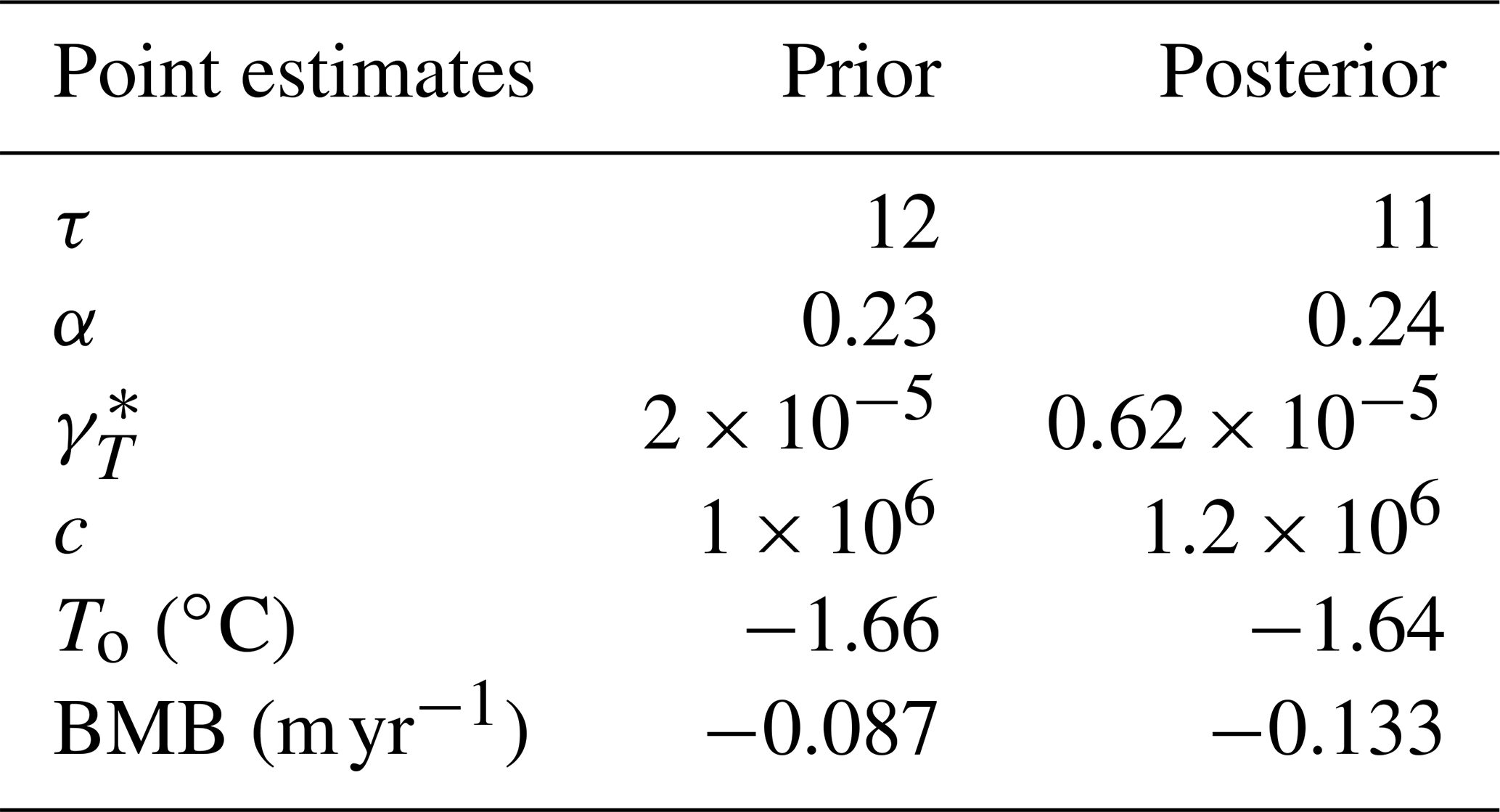
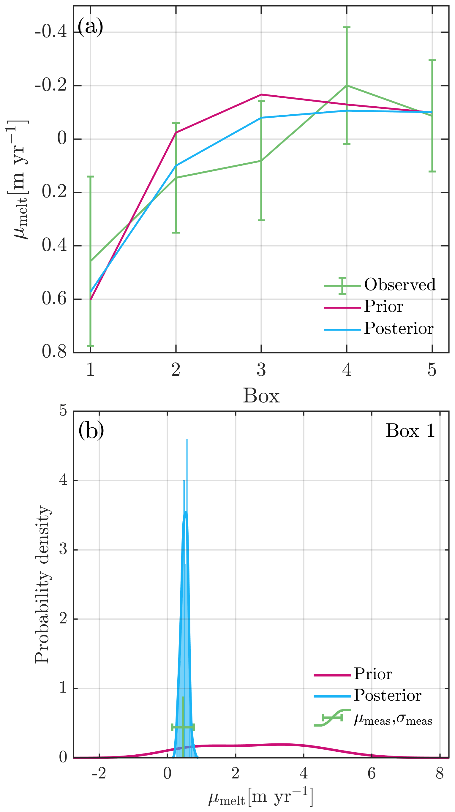
Figure B2 (a) Observed and modelled mean melt rates (μ_melt) for each box in box model melt parameterization. Observations and standard deviations from Moholdt et al. (2014) are shown in green. Pink and blue lines use sample point estimates from Table B1 to compare prior and posterior box melt rates. Prior melt rates (pink) use the same parameters for ${\mathit{\gamma }}_T^{*}$ and c from Reese et al. (2018a) and use mean sample point estimates from our priors for τ and α. The posterior melt rates (blue) use sample point estimates from all parameters from our final posterior distributions. (b) shows the probability distributions of melt rates in Box 1 (closest to the grounding line) using the entire sample set for both priors and posterior. Note the tight distribution around observations (green) for the posterior sample.

To examine the performance of our Bayesian inversion, we compare the total area-integrated basal mass balance i.e. mean specific basal mass balance (see Table B1), and spatially averaged melt rates within each box (Fig. B2a), for both our prior and posterior sample point estimates. Using a priori information (values from priors for τ and α and proposed values for ${\mathit{\gamma }}_T^{*}$ and c from Reese et al., 2018a) yields an area-integrated basal mass balance (BMB) of −0.09 m yr⁻¹. This remains less than half of the BMB from observations −0.26 m yr⁻¹. Using the updated parameter point estimates has brought the BMB closer to observations (−0.13 m yr⁻¹), primarily by improving the mean melt rates in boxes 2 and 3 to within the error of observations (Fig. B2a). Additionally, we take our model optimized velocities (using an inversion with m=3 and n=3) and calculate sub-shelf melt rates from ice flux divergence assuming steady-state conditions, i.e. negligible surface mass balance and no surface thinning or thickening. In this case, BMB is −0.15 m yr⁻¹, which suggests that our point parameter estimates are producing near-steady-state melt rates (−0.13 m yr⁻¹).

We re-evaluate the surrogate model for the entire prior and posterior sample sets to examine the distribution of melt rates in each ocean box. Figure B2b shows the range of initial melt rates (at start year 2000) close to the grounding line (Box 1) that would have occurred in our uncertainty propagation if we had chosen to use non-informative priors, particularly uniform distributions for ${\mathit{\gamma }}_T^{*}$ and c. Given the prior information we have on sub-shelf melt rates (Moholdt et al., 2014), this range of melt rates suggests we would have been sampling unlikely regions of the parameter space. Our Bayesian analysis has successfully tightened the posterior distribution of melt rates, where 5 %–95 % fall within the standard deviation of observations. We can now be confident that our initial melt rates under the ice shelf at the beginning of our forward simulations is reasonable with respect to observations. We note that our approach estimates these distributions at a single snapshot in time and does not take into account variations in these parameters that may occur under future warming, e.g. an increase in the strength of the overturning circulation in ice shelf cavities with warmer ocean temperatures.