Meltwater sources and sinks for multiyear Arctic sea ice in summer

On Arctic sea ice, the melt of snow and sea ice generate a summertime flux of fresh water to the upper ocean. The partitioning of this meltwater to storage in melt ponds and deposition in the ocean has consequences for the surface heat budget, the sea ice mass balance, and primary productivity. Synthesizing results from the 1997–1998 SHEBA field experiment, we calculate the sources and sinks of meltwater produced on a multiyear floe during summer melt. The total meltwater input to the system from snowmelt, ice melt, and precipitation from 1 June to 9 August was equivalent to a layer of water 80 cm thick over the ice-covered and open ocean. A total of 85 % of this meltwater was deposited in the ocean, and only 15 % of this meltwater was stored in ponds. The cumulative contributions of meltwater input to the ocean from drainage from the ice surface and bottom melting were roughly equal.

1 Introduction

During the Arctic summer melt season, copious amounts of relatively fresh water are produced due to snowmelt and sea ice melt. Sources of meltwater are surface snowmelt and ice melt, bottom melt, lateral melt, and rain. This meltwater can be stored in surface melt ponds, be directly deposited in the ocean, or drain from the surface to the ocean either vertically or horizontally. The amount and the fate of this meltwater have implications for the surface energy budget (Hudson et al., 2013), the sea ice mass balance, the thermohaline structure of the upper ocean, and primary productivity in the ice and ocean.

The amount of surface melt water stored in melt ponds influences the summer albedo of sea ice and consequently the surface heat budget. Melt ponds have been studied in field experiments (Perovich et al., 2002a, b; Divine et al., 2015) and through remote sensing imagery (Rösel et al., 2012; Fetterer and Untersteiner, 1998; Webster et al., 2015; Divine et al., 2016; Wright et al., 2020). The morphology and evolution of ponds have been studied using surface topology (Popovic, 2018) and fractals (Hohenegger et al., 2012). Results from pond studies have been incorporated into models (Curry et al., 1995; Flocco et al., 2012; Holland et al., 2012; Schröder et al., 2014). Yet, melt ponds, from a meltwater budget perspective, have received little attention.

In summer, meltwater from bottom melt, lateral melt, drainage from the surface, and rain is input to the upper ocean, freshening and stabilizing it. This meltwater can accumulate in well-defined layers under the ice when there is meltwater input to the upper ocean, bottom topography to trap the meltwater, and calm conditions with little ocean mixing. Under these conditions, false bottoms can form under the sea ice (Untersteiner, 1961; Eicken, 1994; Notz et al., 2003). These false bottoms are below the true ice bottom and are a source of ice production during the melt season. Meltwater accumulation in leads between floes can also develop into well-defined stable layers (Nansen, 1902; Richter-Menge et al., 2001).

The meltwater input impacts the thermohaline structure of the upper ocean, ecosystems, and biogeochemistry. The meltwater layer is a barrier for heat transfer from the ocean to the ice bottom, thus slowing bottom ablation. The upper ocean stratification affects the distribution of microbial and faunal communities and the overall productivity (Gran, 1904; Melnikov et al., 2002; Li et al., 2009).

The importance of the amount and disposition of meltwater in the summer sea ice cover leads directly to several questions. How much meltwater is produced? What are the relative contributions from different sources and how do they change with time? What fraction of surface-produced meltwater is stored in ponds? Here we address these questions by computing a meltwater budget, from a sea ice perspective, over the summer melt season by synthesizing results from the SHEBA experiment (Perovich et al., 1999). Both sources and sinks of meltwater are determined. We examine the time series of meltwater produced through surface snowmelt and ice melt, bottom melt, lateral melt, and rain and explore the sinks of drainage to the ocean and storage in melt ponds.

2 Approach

We calculate the amount and distribution of meltwater sources and sinks during the summer melt cycle of Arctic sea ice by synthesizing results from the SHEBA program. SHEBA was a yearlong (October 1997–October 1998) drift experiment in the Beaufort Sea. The overarching goals of SHEBA were to increase understanding of the ice albedo and cloud radiation feedbacks through interdisciplinary studies of the atmosphere, ice, and ocean and use that understanding to improve models (Perovich et al., 1999). Here, data from the SHEBA field experiment are used to determine contributions from snowmelt, surface melt, bottom melt for both deformed and undeformed ice, lateral melt, and rain, as well as the volume storage in melt ponds.

This work is a synthesis of existing mass balance results from the SHEBA drift experiment. The main SHEBA floe was multiyear ice. The sampling area included undeformed ice, ponded ice, young ridges, and old eroded ridges. The average snow depth just before melt onset was 0.33 m. During summer there was an average of 0.64 m of surface melt and 0.62 m of bottom melt. The data sources for the variables needed for the study are summarized in Table 1. The underlying assumption in this study is that, by design, the SHEBA ensemble of mass balance point measurements provides a statistically representative picture of the SHEBA floe (Perovich et al., 2003). The region of interest for this paper is the SHEBA measurement area of roughly 100 km². The focus is on the period from 1 June 1998 to 9 August 1998. This period was selected since it includes the beginning of the melt season and was the time of maximum surface melt, pond evolution, lateral melting, upper ocean stratification, and data availability.

Table 1 Summary of data sources for meltwater variables.

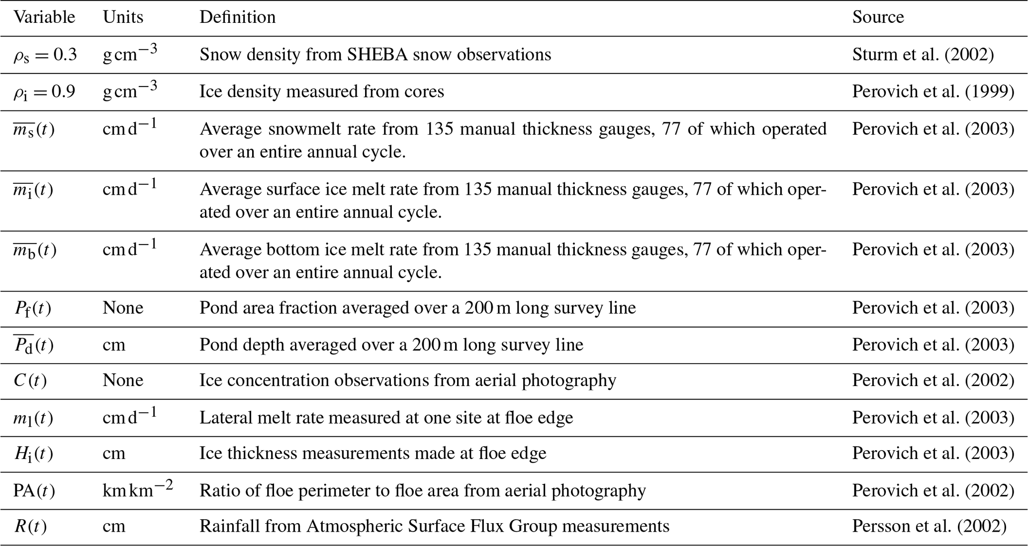
There are two steps to this study. First, the meltwater balance on the ice surface is considered. This includes snowmelt, surface ice melt, rain, storage in melt ponds, and drainage to the ocean. The second step examines the input of meltwater to the ocean. This incorporates the drainage terms as sinks in the surface meltwater budget, plus lateral and bottom ice melt. In this component, contributions from the ice to the ocean are scaled by the ice concentration. The budgets are calculated in terms of an equivalent meltwater layer thickness. Figure 1 is a schematic visualizing the sources and sinks of meltwater during the melt season.

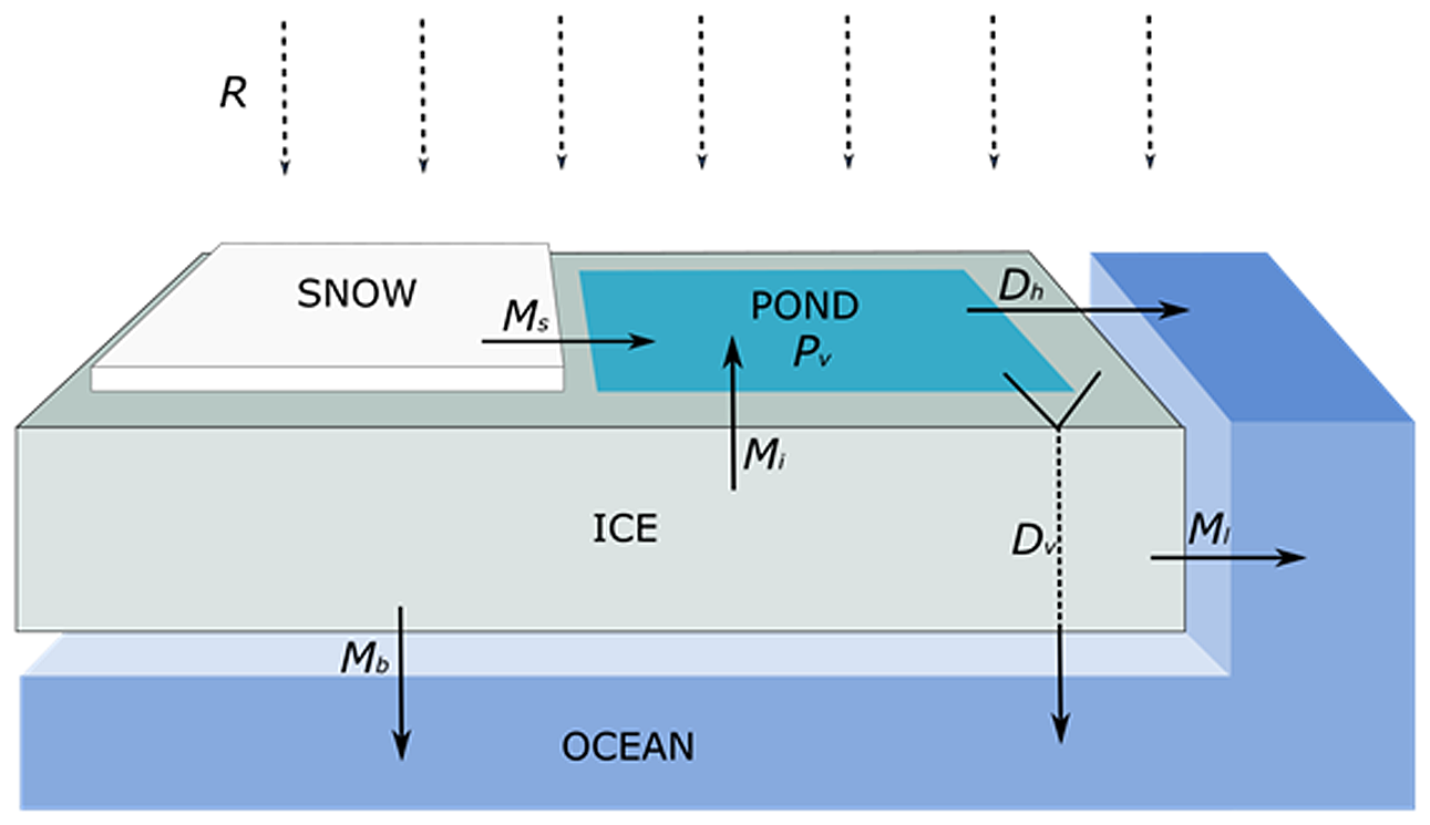
Figure 1 Schematic showing sources and sinks of meltwater used in this analysis. This includes the sources of rain (R), snowmelt (M_s), surface ice melt (M_i), bottom ice melt (M_b), and lateral melt (M_l). It also has the sinks of horizontal drainage (D_h), vertical drainage (D_v), and storage in ponds (P_v).

2.1 Ice surface meltwater balance

There are four sources of meltwater on the surface of the ice: snowmelt (M_s), surface ice melt (M_i), rain (R), and condensation. Condensation is small compared to the other terms and is not considered in this study. There are four sinks for meltwater on the sea ice surface: storage in ponds (P_v), drainage vertically through the ice to the ocean (D_v), drainage horizontally from the ice to cracks and leads (D_h), and evaporation. As was the case for condensation, evaporation is small and neglected in this study. For continuity, surface sources equal surface sinks giving

$$\begin{array}{}\text{(1)}& M_{\mathrm{s}}\left(t\right)+M_{\mathrm{i}}\left(t\right)+R\left(t\right)=P_{\mathrm{v}}\left(t\right)+D_{\mathrm{v}}\left(t\right)+D_{\mathrm{h}}\left(t\right).\end{array}$$

These terms are expressed as a time series of an equivalent layer thickness of meltwater. The meltwater produced by snowmelt is

$$\begin{array}{}\text{(2)}& M_{\mathrm{s}}\left(t\right)={\mathit{\rho }}_{\mathrm{s}}\stackrel{\mathrm{‾}}{m_{\mathrm{s}}}\left(t\right),\end{array}$$

where ρ_s is the density of snow and $\stackrel{\mathrm{‾}}{m_{\mathrm{s}}}\left(t\right)$ is the time series of average snowmelt rate on the floe. The meltwater produced by surface ice melt is

$$\begin{array}{}\text{(3)}& M_{\mathrm{i}}\left(t\right)={\mathit{\rho }}_{\mathrm{i}}\stackrel{\mathrm{‾}}{m_{\mathrm{i}}}\left(t\right).\end{array}$$

ρ_i is the density of ice, and $\stackrel{\mathrm{‾}}{m_{\mathrm{i}}}\left(t\right)$ is the time series of average surface ice melt rate on the floe. R(t) is the time series of rain during the summer. The meltwater stored in ponds is

$$\begin{array}{}\text{(4)}& P_{\mathrm{v}}\left(t\right)=P_{\mathrm{f}}\left(t\right)\stackrel{\mathrm{‾}}{P_{\mathrm{d}}}\left(t\right).\end{array}$$

P_f(t) is the time series of pond fraction on the floe. $\stackrel{\mathrm{‾}}{P_{\mathrm{d}}}\left(t\right)$ is the time series of the average pond depth.

The drainage terms are a challenge, as SHEBA had no direct measurements of drainage. As a result, vertical and horizontal drainage are combined and treated as a residual of the other terms in Eq. (1). This treatment of the drainage term also accounts for simultaneous vertical and horizontal drainage, which can occur at times (Eicken et al., 2002).

2.2 Input to the upper ocean

Meltwater drainage is important when considering meltwater input to the ocean. The total meltwater input to the ocean, O_fw(t), is a sum of the sources: horizontal and vertical drainage, bottom melting, lateral melting M_l(t), and rain falling on leads.

$$\begin{array}{ll}{\displaystyle }{O}_{\text{fw}}\left(t\right)=& {\displaystyle }C\left(t\right)\left(D_{\mathrm{h}}\right(t)+D_{\mathrm{v}}(t\left)\right)+C\left(t\right)M_{\mathrm{b}}\left(t\right)\\ \text{(5)}& {\displaystyle }& {\displaystyle }+C\left(t\right)M_{\mathrm{l}}\left(t\right)+(\mathrm{1}-C(t\left)\right)R\left(t\right)\end{array}$$

Here, terms are scaled by the ice concentration time series, C(t), to account for meltwater contributions spread over an area that includes both the ice and the leads. Bottom melting is

$$\begin{array}{}\text{(6)}& M_{\mathrm{b}}\left(t\right)={\mathit{\rho }}_{\mathrm{i}}\stackrel{\mathrm{‾}}{m_{\mathrm{b}}}\left(t\right).\end{array}$$

$\stackrel{\mathrm{‾}}{m_{\mathrm{b}}}\left(t\right)$ is the time series of average surface ice melt rate on the floe. Lateral melting is expressed as

$$\begin{array}{}\text{(7)}& M_{\mathrm{l}}\left(t\right)={\mathit{\rho }}_{\mathrm{i}}{m}_{\mathrm{l}}\left(t\right)H_{\mathrm{i}}\left(t\right)\text{PA}\left(t\right).\end{array}$$

m_l(t) is the lateral melt rate, and H_i(t) is the ice thickness at the floe edge. PA(t) is the floe perimeter per unit area of the floe (units of km km⁻²).

3 Results

3.1 Ice surface meltwater balance

The daily meltwater input to the ice surface from snowmelt, surface ice melt, and rain is plotted in Fig. 2. In early June, the largest contribution comes from snowmelt reaching a maximum of about 0.6 cm d⁻¹. As the snow cover melts away, the snow contribution decreases and the ice contribution begins to increase. The surface ice melt contribution increases through June into July, reaching a peak of 2 cm d⁻¹ on 20 July and rapidly decreasing afterward. It was often foggy and misting during the summer, but the amount of precipitation during these periods was small. We included the only two significant rainfall events: 2 cm of rain around 5–6 July and 1 cm of rain around 26–27 July.

Figure 2 Time series of meltwater input from snowmelt, surface ice melt, and rain.

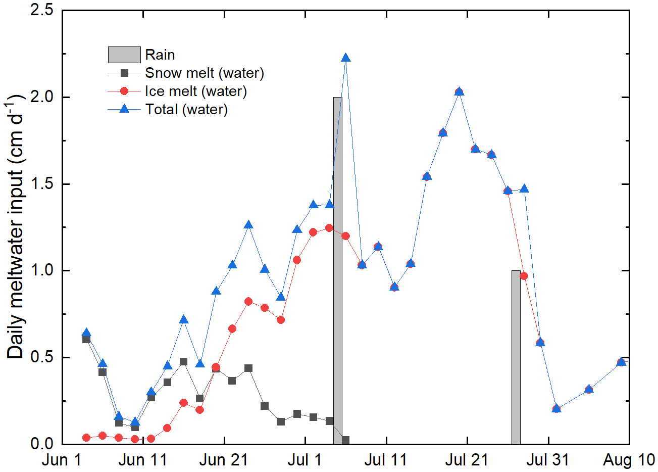
The time series of melt pond fraction and average pond depth is shown in Fig. 3. Pond measurements along the survey line started about 10 d after the initial melt pond formation. The pond survey on 20 June coincides with the first pond area maximum as observed from aerial photography (Perovich et al., 2002). The pond fraction decreased from 20 to 25 June, due to drainage. This was primarily due to vertical drainage associated with high ice permeability (Eicken et al., 2002). Afterwards, there was a steady increase in pond fraction and depth through early August, reaching maximum values of 0.37 for fraction and 39 cm for average depth.

Figure 3 Time series of average pond depth (P_d(t)) and pond fraction (P_f(t)) along a 200 m long survey line.

The time series of cumulative meltwater input to the sea ice surface and the amount stored in ponds is plotted in Fig. 4. As before, the cumulative water input is presented as the equivalent depth of a layer of meltwater placed on top of the floe. Initially, the fraction of the surface meltwater stored in ponds was 0.25. It rapidly decreased to 0.07 in only 5 d as a result of vertical drainage and a reduction in pond coverage. After that, the fraction stored in ponds steadily increased to a final value of 0.23 on 8 August. Throughout the melt season, the majority of the surface meltwater is drained into the upper ocean rather than being stored in ponds. The time series of the cumulative meltwater drained both horizontally and vertically is the difference between the total cumulative input and the amount stored in ponds. By 8 August, the drained amount was equal to a 50 cm layer of meltwater on the ice surface. There was a steady increase in the amount drained from 20 June to 27 July followed by a gradual tapering to 8 August. During summer, the surface melt rates, pond depths, and pond areas were continually changing. However, even with all those changes, there was a consistency in drainage. From 20 June to 23 July, there was an average increase of 1.02 cm d⁻¹ and a standard deviation of 0.09 cm d⁻¹. This provided a steady influx of meltwater from the ice surface into the ocean.

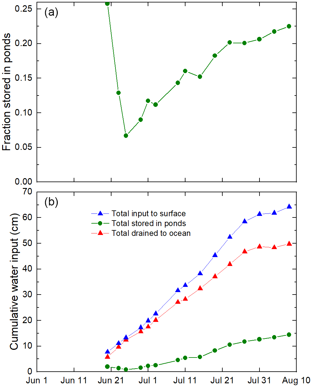
Figure 4 Time series of the fraction of surface water input stored in ponds (a), and cumulative surface water input, storage in ponds (P_v), and drained to ocean (b).

3.2 Input to the upper ocean

The time series of meltwater input to the upper ocean (O_fw(t)) is calculated using Eq. (5). Here the meltwater input represents a layer over the area covered by both the ice and leads. Meltwater inputs from the ice are scaled by the ice concentration to account for the total area of ice plus leads. Helicopter-based aerial photography surveys were used to determine the time series of ice concentration at SHEBA as shown in Fig. 5 (Perovich et al., 2002). These surveys sampled areas typically covering hundreds of square kilometers. In mid-June, the ice concentration dropped to 0.8 and stayed between 0.8 and 0.85 for the remainder of the period of interest.

Rain falling on leads was a very minor component of the meltwater input to the upper ocean. After adjusting for ice concentration, the cumulative input was only 0.13 cm.

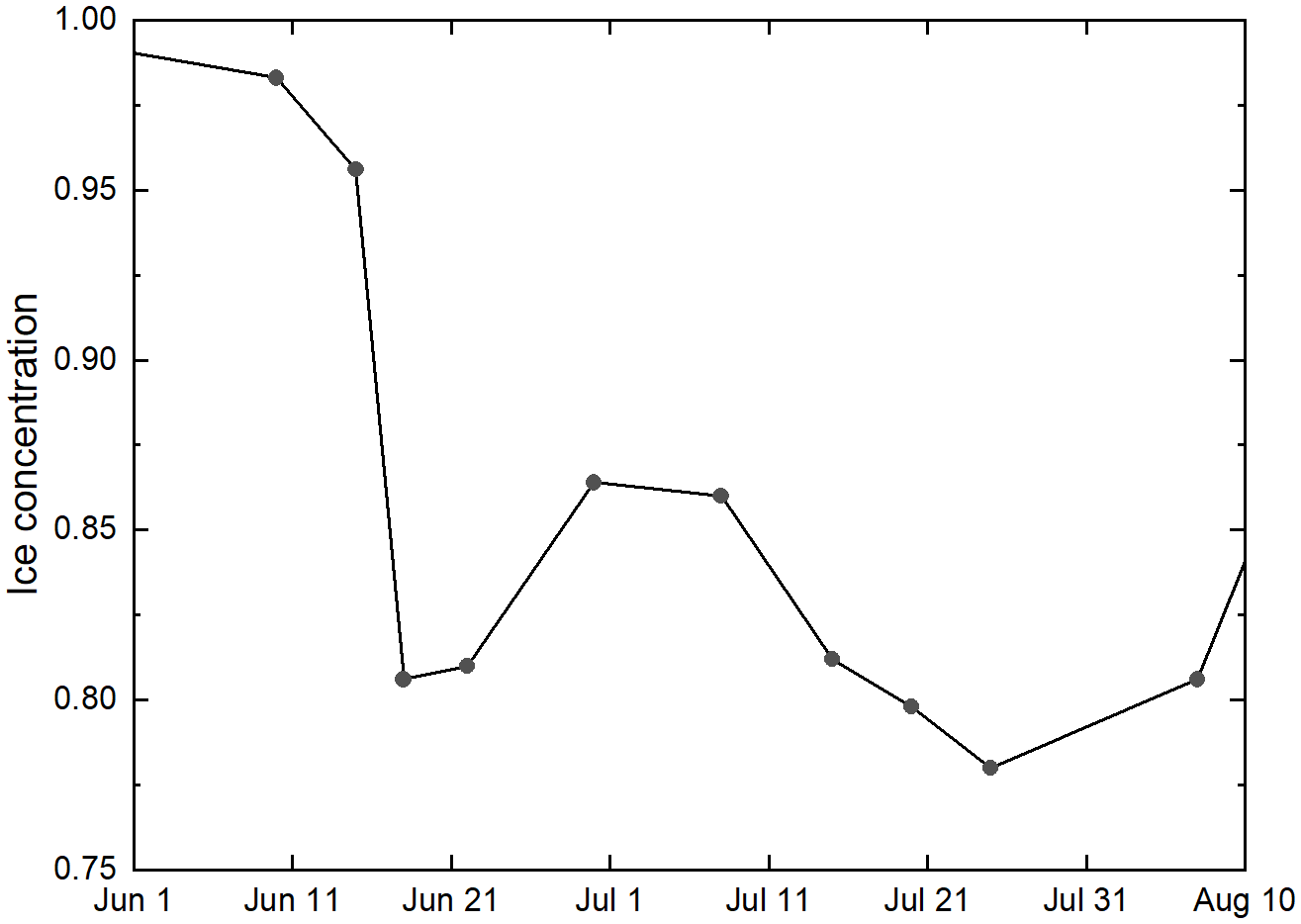
Figure 5 Time series of ice concentration determined from aerial photographs, C(t) (Perovich et al., 2002).

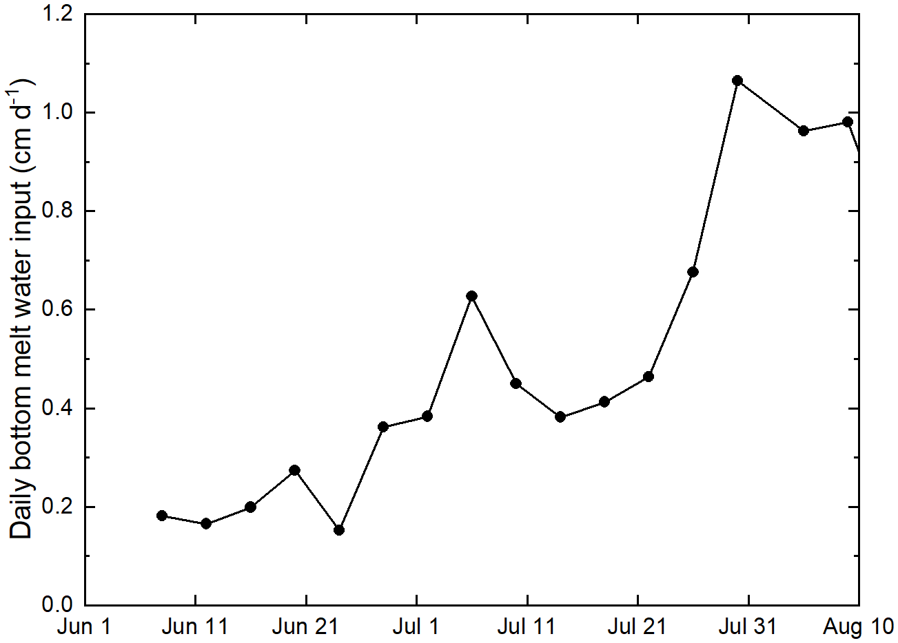
The contribution from surface drainage is simply the residual from Eq. (1), as shown in Fig. 4, scaled by the ice concentration. The average bottom melt rate ($\stackrel{\mathrm{‾}}{m_{\mathrm{b}}}$) is computed using the same array of thickness gauges used to determine surface melt rates (Perovich et al., 2003). Initially the average bottom melt rate was only about 0.2 cm d⁻¹ (Fig. 6). There was a gradual increase over the summer, reaching a peak of 1.1 cm d⁻¹ in late July after the under-ice meltwater layer was removed by mixing caused by ice motion.

Figure 6 Time series of bottom melt rates, M_b(t) (Perovich et al., 2003).

Determining the contribution from lateral melting is somewhat complicated. During SHEBA, there was only one site where a complete time series of lateral melting was measured. We assume that this one site is representative of the entire floe. Lateral melting can result in wall profiles with overhanging lips, shelves, and scallops (Perovich et al., 2003). Lateral melt rates were determined by measuring the change in wall area and applying it to a hypothetical vertical wall generating a lateral melt rate. The ice thickness at the floe edge was measured using a thickness gauge. The ratio of floe perimeter to floe area was used to compare lateral melting to surface and bottom melting. This ratio was determined from the analysis of aerial photography where both the floe perimeter and floe area were computed.

The time series of lateral melt rate, ice thickness, and the ratio of floe perimeter to area are plotted in Fig. 7. There were large changes starting on 21 July. The floe perimeter to area ratio increased by roughly a factor of 4, while the lateral melt increased from 4 to 22 cm d⁻¹. During this period, ice motion increased from a few cm s⁻¹ to 40 cm s⁻¹, floes broke up, and heat stored in leads was transported to the ice edge, enhancing lateral melting (Richter-Menge et al., 2001). The meltwater stored in the upper few meters of the lead was mixed downward (Richter-Menge et al., 2001).

Figure 7 Time series of thickness at the ice edge, lateral melt rate (M_l(t)), and the ratio of floe perimeter to area PA(t).

The contributions to upper ocean meltwater input from surface drainage, bottom melt, and lateral melt are plotted in Fig. 8. For most of the summer, the largest contribution was from drainage through the ice. By 9 August, though, the contributions from surface drainage and bottom melt were equal. The lateral melt contribution was the smallest. The cumulative total meltwater input increase was well represented (R²=0.997) by a second-order polynomial of the form

$$\begin{array}{}\text{(8)}& O_{\text{fw}}=\mathrm{0.0099}{t^{\prime }}^{\mathrm{2}}+\mathrm{0.469}{t}^{\prime }+\mathrm{0.0396},\end{array}$$

where t^′ is the number of days since 8 June.

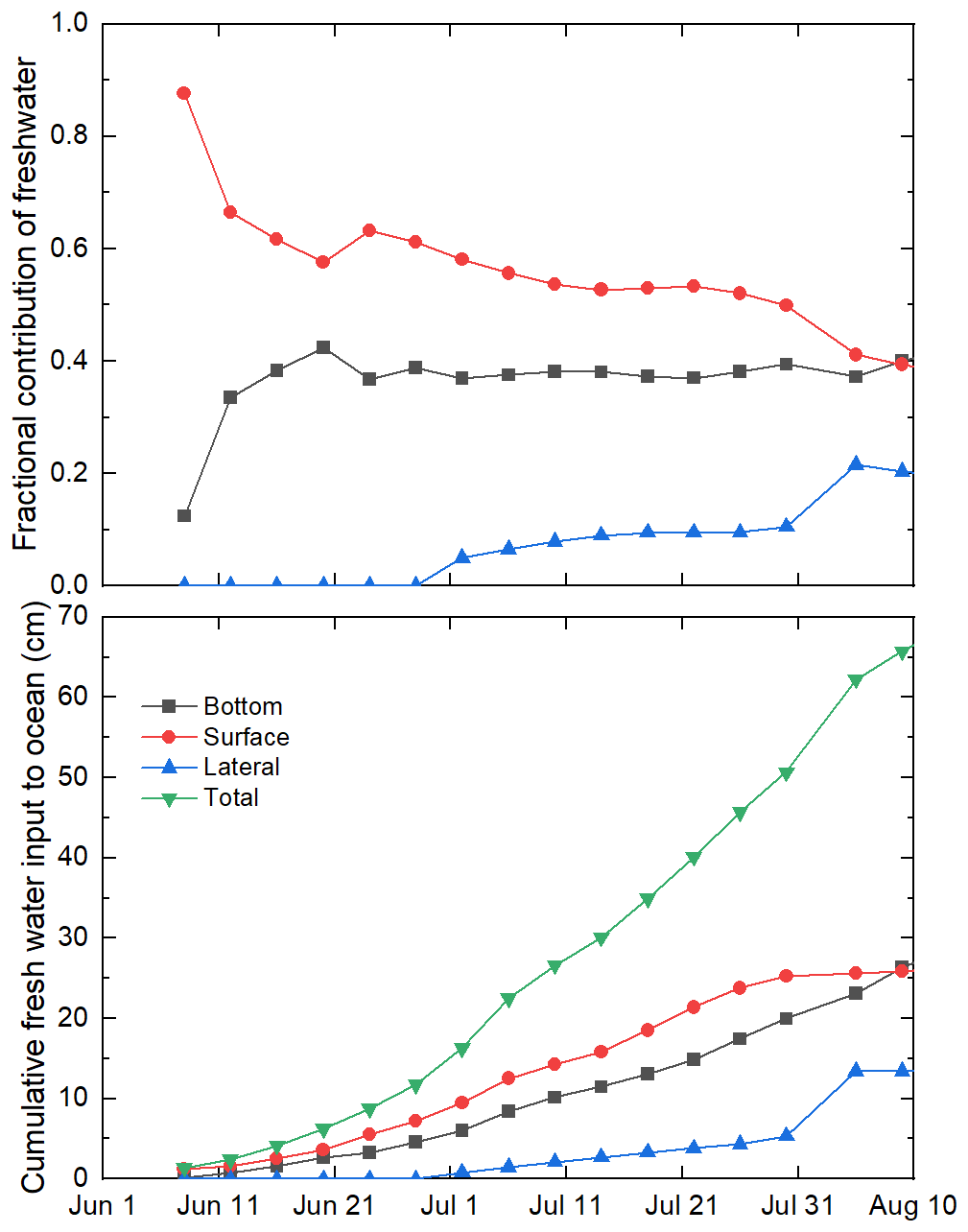
Figure 8 Upper ocean meltwater budget. Time series of fresh input to the ocean with contributions from lateral melting, bottom melting, and surface melting. The total input is also plotted. The melt contributions have been adjusted by the ice concentration.

4 Discussion and conclusions

From 1 June to 9 August, the total meltwater produced was equal to a layer 80 cm thick and the input to the ocean was equivalent to a layer 68 cm thick. This suggests that most of the meltwater produced over the Arctic summer was deposited in the ocean; on 9 August, only 15 % of the meltwater produced was stored in ponds. This does not mean that on 9 August there was a 68 cm thick meltwater layer under the ice. The meltwater could be stored under the ice, in leads, and mixed deeper in the ocean. The fate of this meltwater depends on multiple factors including ice–ocean interaction, ice bottom topography, the dynamics of the ice cover, and the horizontal and vertical partitioning of drainage.

This paper determined the amount of drainage from the ice surface to the ocean, but it was unable to delineate between horizontal and vertical drainage. This misses an important distinction since meltwater input to leads or to the underside of the ice will have different behaviors and impacts. Horizontal transport will fill leads with meltwater, creating a stable surface layer that can be warmed by solar heating (Richter-Menge et al., 2001). Lateral melting also contributes directly to freshening of leads. This results in a stable surface layer in leads affecting ocean–ice heat transfer and ocean–atmosphere gas exchange. Opening and closing of leads will mix this meltwater layer, transport heat to the ice edge, and force it under the ice. In contrast, vertical drainage can form a meltwater layer under the ice leading to the formation of false bottoms, isolate the ice from the ocean, and impact heat and nutrient fluxes. Ice motion and wind forcing can mix and dissipate this layer.

While we cannot quantitatively define the distribution of vertical to horizontal drainage, we can make some qualitative observations about the timing of when vertical vs. horizontal drainage occurred. Ponds above freeboard provide hydrostatic head to promote vertical drainage. In early June, most ponds were above freeboard. In mid-June, there was rapid drainage and a decrease in pond coverage. This occurred when the ice warmed, its brine volume increased, and it became permeable enough for vertical drainage to occur (Eicken et al., 2002). Also at this time, ponds were amorphous with no established horizontal drainage system to link ponds to the floe edge (see Fig. 9).

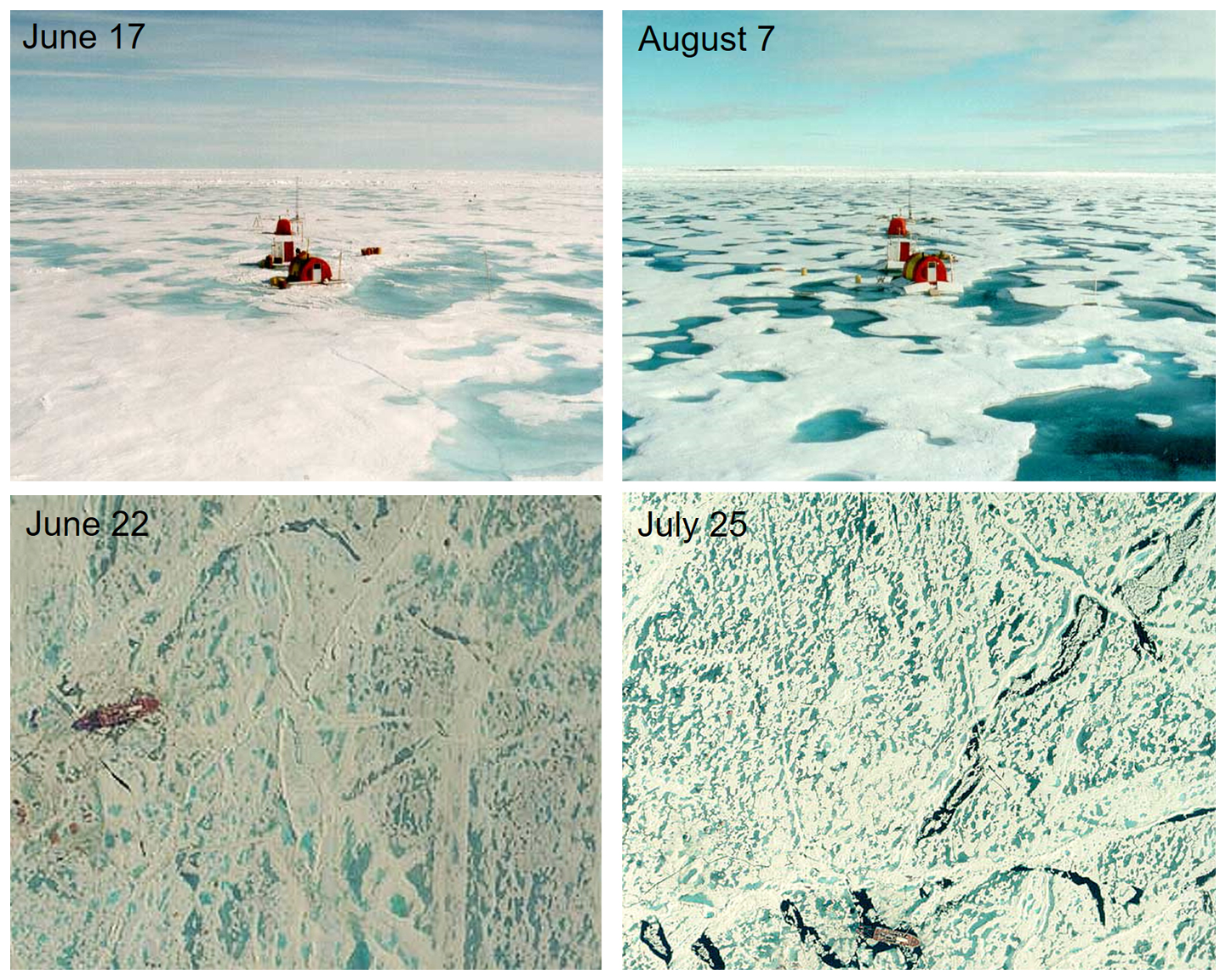
Figure 9 Surface and aerial photographs of Ice Station SHEBA at different stages of pond evolution, earlier and later in the melt season. The CCG Des Groseilliers (98 m length) is visible in the lower photographs.

By early August, the situation had changed. Many of the ponds were at sea level, with no hydrostatic head. There was an elaborate melt channel network connecting melt ponds to each other and to the ice edge (Hohenegger et al., 2012) (see Fig. 9). The lead fraction had increased from 0.03 to 0.18. Floes had broken, increasing the floe perimeter from 7.4 km km⁻² (22 June) to 45.0 km km⁻² (7 August). At this stage, horizontal drainage increased.

It is possible to generate a rough estimate of the horizontal to vertical drainage for a brief period. During SHEBA, vertical profiles of temperature and salinity were made at a lead site. This showed the gradual buildup of meltwater and heat in the lead and how a dynamic ice event mixed this upper layer and greatly enhanced lateral melting (Richter-Menge et al., 2001). From 10 to 20 July there was a steady deepening of the meltwater layer from 70 to 120 cm. This occurred during a quiescent period with little winds and little ice motion. Making a few assumptions, we use the 10 d, 50 cm increase in the meltwater layer to estimate the fraction of surface meltwater that is horizontally drained.

We assume that (i) the meltwater in leads only comes from lateral melting and horizontal drainage, (ii) all lateral melting contributes to freshening of the lead, (iii) no meltwater in the lead is lost under the ice or deeper in the ocean, and (iv) measurements at the lead site are representative of the broader area. Using these assumptions, the increased depth of the meltwater layer in the lead from 10 to 20 July is equal to the contribution from lateral melting and horizontal drainage. During this period, the ice concentration was 0.95, giving a concentration-adjusted lead freshening of 2.5 cm. The contribution from lateral melt during this period was 1.4 cm, giving a contribution from horizontal drainage of 1.1 cm. Adjusted by concentration, the surface meltwater production during this period was 13.8 cm, with 3.7 cm being stored in ponds and 10.1 cm drained. Thus, for this period, it is estimated that 11 % of the drainage was horizontal.

There were no measurements of the thermohaline structure of the top few meters of the upper ocean directly under the ice during SHEBA. Future studies should include routine profiles of temperature and salinity under the ice at multiple locations. This would show the buildup and erosion of the meltwater layer under the ice.

These results are from a multiyear floe in the Beaufort Sea during the summer of 1998. Future work should explore the spatial variability of the meltwater seasonal cycle and changes over time. Some information can be obtained from autonomous buoys. For example, autonomous sea ice mass balance measurements in the Beaufort Sea indicate large increases in bottom melting in recent years (Perovich and Richter-Menge, 2015). This has resulted in a larger meltwater contribution from bottom melt and a larger fraction of the meltwater production deposited in the ocean. While the contributions from surface and bottom melt are straightforward to measure autonomously, the contributions from lateral melting and the amount stored in melt ponds are more challenging. This gap could be partially filled by sensors measuring temperature and salinity profiles in the upper few meters of the ocean directly beneath the ice. Aerial and satellite imagery aids in extending results to larger scales.

This study was conducted on a multiyear floe. However, more of the ice cover is first-year ice, with less snow, thinner ice, and flatter topography. Future work needs to examine the impact of these changes on meltwater partitioning. Field experiments covering the full seasonal cycle, such as the Multidisciplinary drifting Observatory for the Study of Arctic Climate (MOSAiC) expedition (Shupe et al., 2020), are the optimal way to determine the evolution of the sources and sinks of meltwater on a mixture of first- and second-year ice.