the Creative Commons Attribution 4.0 License.
the Creative Commons Attribution 4.0 License.
 | 06 Aug 2021
The 21st-century fate of the Mocho-Choshuenco ice cap in southern Chile
Matthias Scheiter
Marius Schaefer
Eduardo Flández
Deniz Bozkurt
Ralf Greve
Glaciers and ice caps are thinning and retreating along the entire Andes ridge, and drivers of this mass loss vary between the different climate zones. The southern part of the Andes (Wet Andes) has the highest abundance of glaciers in number and size, and a proper understanding of ice dynamics is important to assess their evolution. In this contribution, we apply the ice-sheet model SICOPOLIS (SImulation COde for POLythermal Ice Sheets) to the Mocho-Choshuenco ice cap in the Chilean Lake District (40∘ S, 72∘ W; Wet Andes) to reproduce its current state and to project its evolution until the end of the 21st century under different global warming scenarios. First, we create a model spin-up using observed surface mass balance data on the south-eastern catchment, extrapolating them to the whole ice cap using an aspect-dependent parameterization. This spin-up is able to reproduce the most important present-day glacier features. Based on the spin-up, we then run the model 80 years into the future, forced by projected surface temperature anomalies from different global climate models under different radiative pathway scenarios to obtain estimates of the ice cap's state by the end of the 21st century. The mean projected ice volume losses are 56±16 % (RCP2.6), 81±6 % (RCP4.5), and 97±2 % (RCP8.5) with respect to the ice volume estimated by radio-echo sounding data from 2013. We estimate the uncertainty of our projections based on the spread of the results when forcing with different global climate models and on the uncertainty associated with the variation of the equilibrium line altitude with temperature change. Considering our results, we project a considerable deglaciation of the Chilean Lake District by the end of the 21st century.
- Article
(5736 KB) - Full-text XML
- BibTeX
- EndNote


Most glaciers and ice caps in the Andes are currently thinning and retreating (e.g. Braun et al., 2019), and rates of mass loss are increasing in many places (Dussaillant et al., 2019). In the southernmost part of the Andes (36–56∘ S), which is called the Wet Andes or Patagonian Andes in the literature (Lliboutry, 1998), the highest number of glaciers are found, and large ice fields such as the Northern Patagonia Ice Field, Southern Patagonia Ice Field, and Cordillera Darwin are located in this region. The specific mass losses observed or inferred for the glaciers of the Wet Andes are the highest in the Andes (Dussaillant et al., 2019; Braun et al., 2019) and among the highest of all glacier regions worldwide (Zemp et al., 2019).
The maritime climate of the Wet Andes is characterized by high precipitation rates of up to 10 m yr−1 on the windward side and rather mild temperatures with freezing levels generally above 1 km above mean sea level with an overall modest seasonality (Garreaud et al., 2013). This leads to an exceptionally high mass turnover (Schaefer et al., 2013, 2015, 2017) and high flow speeds for the glaciers in the region (Sakakibara and Sugiyama, 2014; Mouginot and Rignot, 2015). In addition to climate forcings, other important contributors to glacier change in the region are ice dynamics and frontal ablation. Ice-flow models incorporate these processes and are therefore appropriate tools to project the future behaviour of the glaciers of the Wet Andes.
Only a few studies have tried to project future behaviour of Andean glaciers. Réveillet et al. (2015) modelled Zongo Glacier (16∘ S) in the tropical Andes using the three-dimensional full-Stokes model Elmer/Ice (developed by Gagliardini et al., 2013). They projected volume losses between 40 % and 89 % by the end of this century under the RCP2.6 and RCP8.5 scenarios, respectively. In the Wet Andes, Möller and Schneider (2010) projected an area loss of 35 % of Glaciar Noroeste, an outlet glacier of the Gran Campo Nevado ice cap (53∘ S), by the end of the 21st century using a degree-day model and volume-area scaling relationships. Schaefer et al. (2013) modelled the surface mass balance (SMB) of the Northern Patagonian Ice Field in the 21st century under the A1B scenario (of Assessment Report 4 from the Intergovernmental Panel on Climate Change, IPCC; comparable to RCP6.0). They projected a strongly decreasing SMB until the end of the 21st century mainly due to an increase in surface temperature by the middle of the century and a decrease in accumulation towards the end of the century. Collao-Barrios et al. (2018) infer important committed mass loss of San Rafael Glacier under current climate applying the Elmer/Ice flow model with fixed glacier outlines.
In this contribution, our first objective is to reproduce the present-day behaviour of the Mocho-Choshuenco ice cap in the northern part of the Wet Andes (40∘ S) using the ice-sheet model SICOPOLIS (SImulation COde for POLythermal Ice Sheets) (Greve, 1997a, b). To this end, we make use of a newly developed SMB parameterization scheme and glaciological data obtained on the ice cap to calibrate the model and reproduce its current state. Our second objective is to project the behaviour of the Mocho-Choshuenco ice cap through the course of the 21st century to provide one of the first constraints on future glacier dynamics in the Wet Andes. For this aim, we make use of temperature projections from 23 global climate models (GCMs) participating in the Coupled Model Intercomparison Project phase 5 (CMIP5) (Taylor et al., 2012) under low (RCP2.6), medium (RCP4.5), and high (RCP8.5) emission scenarios as input to SICOPOLIS.
We begin this paper by describing the observational data and methods (Sect. 2). In Sect. 3, we present the results. First, we validate the model spin-up using observed SMB, glacier outlines, ice thickness, and flow speed. We then present the evolution of ice cap extension and volume during the 21st century as obtained through different emission scenarios. Then, in Sect. 4, we discuss our results, compare them to previous studies, and analyse the limitations of our approach. We conclude the paper by summarizing the main findings in Sect. 5.
2.1 Observational data
The ice cap on which we focus in this study covers the Mocho-Choshuenco volcanic complex, which is located at 40∘ S, 72∘ W (see inset map in Fig. 1). Over the last 20 years, climatological and glaciological observations have been made on the ice cap (Rivera et al., 2005; Schaefer et al., 2017). SMB data were obtained through the traditional glaciological method on a stake network on the south-eastern part of the ice cap (red stars in Fig. 1). These measurements reported by Schaefer et al. (2017) yielded an average negative SMB of (metre water equivalent per year) with a high mass turnover of around (see Sect. 2.4). This high mass turnover is a consequence of the interaction between high precipitation rates leading to high accumulation rates and high temperatures leading to high melt rates. In this respect, climatological data (2006 to 2015) indicate that the annual mean temperature was 2.6 ∘C at an automatic weather station (green circle in Fig. 1) at an elevation of 2000 m and therefore close to the typical equilibrium line altitude (ELA) (Schaefer et al., 2017). Mean annual precipitation over the same period was around 4000 mm yr−1 in Puerto Fuy at an elevation of 600 m to the north of the volcano, and orographic precipitation effects lead to a relatively high amount of precipitation on the ice cap.

Figure 1Overview map of the Mocho-Choshuenco ice cap with significant geographic features and measurement sites. The contour line spacing is 50 m. East and north are in UTM S18. Background: Landsat image (22 February 2015). Inset map shows location in South America.
At some of the mass balance stakes (red stars with inner black dots in Fig. 1), high precision GPS measurements were made in July and October 2013 to infer surface flow velocity (Geoestudios, 2013), and the observed velocities are shown in Table 1. Further measurements include ground penetrating radar (GPR) transects (green lines in Fig. 2a) over most parts of the ice cap (Geoestudios, 2014). Through inverse distance weighting interpolation over the whole ice cap, a total ice volume of 1.038 km3 was obtained (Geoestudios, 2014). The interpolated ice thickness map was subtracted from a digital elevation model (TanDEM WorldDEM™, acquired between 2012 and 2014) to yield a bedrock topography (Flández, 2017). We use this topography as the base of the ice cap in the simulations we perform with SICOPOLIS.
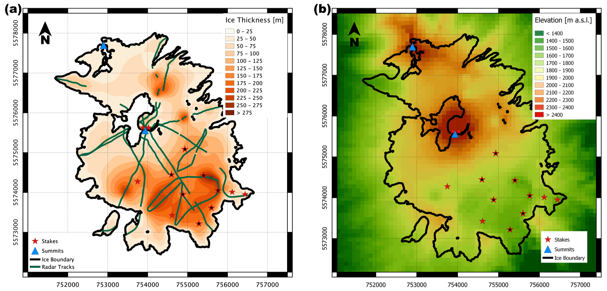
Figure 2(a) Ground penetrating radar (GPR) transects shown in green lines together with the interpolated ice thickness. (b) Bedrock topography obtained after subtracting the interpolated ice thickness from surface elevation. This topography is used as the ice cap base in our simulations.
Table 1Comparison between simulated and observed velocities at stakes where velocity observations are available from Geoestudios (2013).

2.2 SICOPOLIS
The three-dimensional, dynamic and thermodynamic model SICOPOLIS was originally created in a version for the Greenland ice sheet (Greve, 1997a, b). Since then, the model has been developed continuously and applied to problems of past, present, and future glaciation of Greenland, Antarctica, the entire Northern Hemisphere, the polar ice caps of the planet Mars, and other places, resulting in more than 120 publications in the peer-reviewed literature (http://www.sicopolis.net, last access: 3 August 2021). The model supports the shallow-ice approximation (SIA) for slow-flowing grounded ice, hybrid shallow-ice–shelfy stream dynamics for fast-flowing grounded ice, and the shallow-shelf approximation for floating ice (Bernales et al., 2017), as well as several thermodynamics solvers (Blatter and Greve, 2015; Greve and Blatter, 2016).
Mainly developed for ice sheets, the smallest ice body to which SICOPOLIS has been applied so far is the Austfonna Ice Cap, for which Dunse et al. (2011) reproduced the observed cyclic surge behaviour under constant, present-day climate conditions. For this study, we adapted SICOPOLIS v5-dev (Greve and SICOPOLIS Developer Team, 2021) for the Mocho-Choshuenco ice cap in SIA mode. The horizontal resolution is 100 m. In the vertical, we use terrain-following coordinates (sigma transformation) with 81 layers. The time step for the numerical integration is 0.01 years. We employ a standard Glen flow law with a stress exponent of n=3. Basal sliding is modelled by a linear sliding law,
where vb is the basal sliding velocity, τb the basal drag, and Cb the sliding coefficient. The value of the latter is determined by the calibration procedure of the present-day spin-up (see Sect. 3.1). Since Mocho-Choshuenco is a temperate ice cap, we do not solve the energy balance equation. Rather, we keep the temperature at a constant value of 0 ∘C (precisely speaking, and for technical reasons only as SICOPOLIS does not allow an all-temperate ice body, ). The rate factor is set to the value recommended by Cuffey and Paterson (2010) for 0 ∘C, which is . To ensure proper mass conservation despite the steep slopes and rugged bed topography, we use an explicit solver for the ice thickness equation that discretizes the advection term by a mass-conserving scheme in an upwind flux form (Calov et al., 2018).
2.3 Aspect-dependent SMB parameterization
SICOPOLIS incorporates a linear altitude-dependent SMB parameterization which is visualized in Fig. 3a and can be described by the following formula:
Here, ELA is the equilibrium line altitude, z(C) is the evolving ice surface elevation of a specific grid cell C, M0 denotes the mass balance gradient, and S0 is maximum SMB.
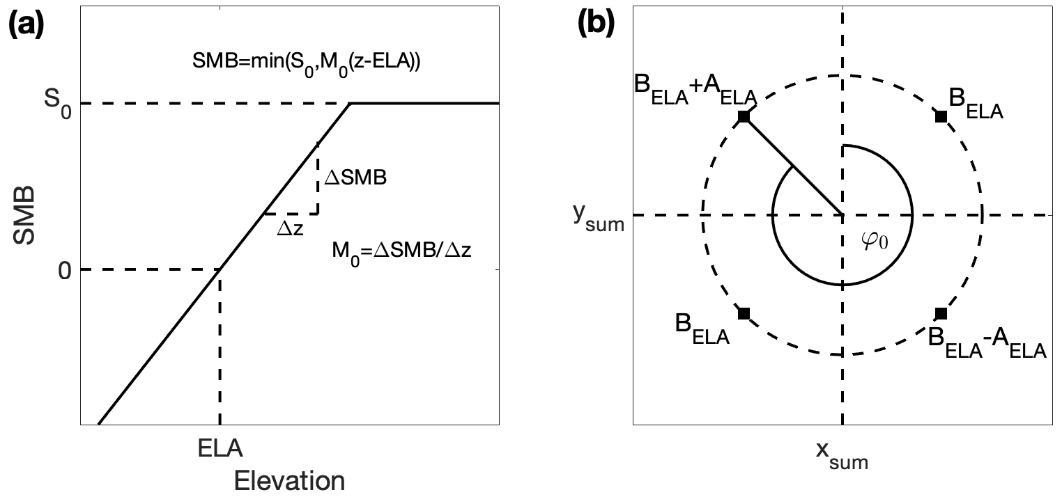
Figure 3(a) Elevation-dependent SMB parameterization. SMB increases linearly with elevation until an upper bound S0 and stays constant at higher elevations. (b) Aspect-dependent SMB parameterization. Equilibrium line altitude (ELA) takes a minimum and maximum on two opposite directions (BELA±AELA) and their mean (BELA) on perpendicular directions. φ0 is a direction offset to rotate the values according to the atmospheric conditions. In this visualization, φ0 is set to 315∘, the value used in this study, and (xsum,ysum) indicates the position of Mocho's summit.
From the simulations performed by Flández (2017) on the Mocho-Choshuenco ice cap, it becomes apparent that the simple altitude-dependent SMB parameterization in Eq. (2) is not detailed enough to account for small-scale SMB variations in the ice cap. In particular, SMB should be lower in the north-western part than in the south-eastern part of the ice cap due to the aspect dependence of solar radiation and snow redistribution (wind drift) which during precipitation events predominantly blows from the north-west. We therefore employ a new parameterization which is illustrated in Fig. 3b. With Mocho's summit in the centre, ELA should have a maximum BELA+AELA in the direction φ0, a minimum BELA−AELA in the opposite direction, and a mean value BELA in the two perpendicular directions.
These values can be summarized in a cosine function in φ with the direction of maximum ELA φ0, the amplitude AELA, and an offset of the average ELA BELA:
BELA is used to shift the ELA to the desired mean altitude, φ is the cardinal direction of a point with respect to the summit, and it can be calculated by
where arctan2 denotes the two-argument arctangent, and x and y are the distances in the two directions from a grid point to the summit location (xsum,ysum).
2.4 Transient spin-up
Before being able to make future projections for the Mocho-Choshuenco ice cap, we first aim to reproduce its current state. Due to the observed negative SMB at present, we aim to build a transient spin-up that represents a shrinking ice cap. This is achieved in two steps: first, we build a theoretical steady state of the ice cap in the late 1970s and then run the model from 1979 to 2013 with ERA5 near-surface air temperature data (see Fig. 4). This 35-year period is justified by the turnover time τ, which is a typical timescale for a glacier defined by
where [H] is the typical ice thickness and [SMB] the typical SMB (e.g. Greve and Blatter, 2009). By taking (where Vobs=1.038 km3 is the observed ice volume and Aobs=15.1 km3 the observed area) and (computed as the mean of the absolute values from the observed SMB at the stakes), we obtain τ≈27 years. This is slightly less than the 35-year period of ERA5 data, which therefore should be sufficient to produce a valuable spin-up for the year 2013.
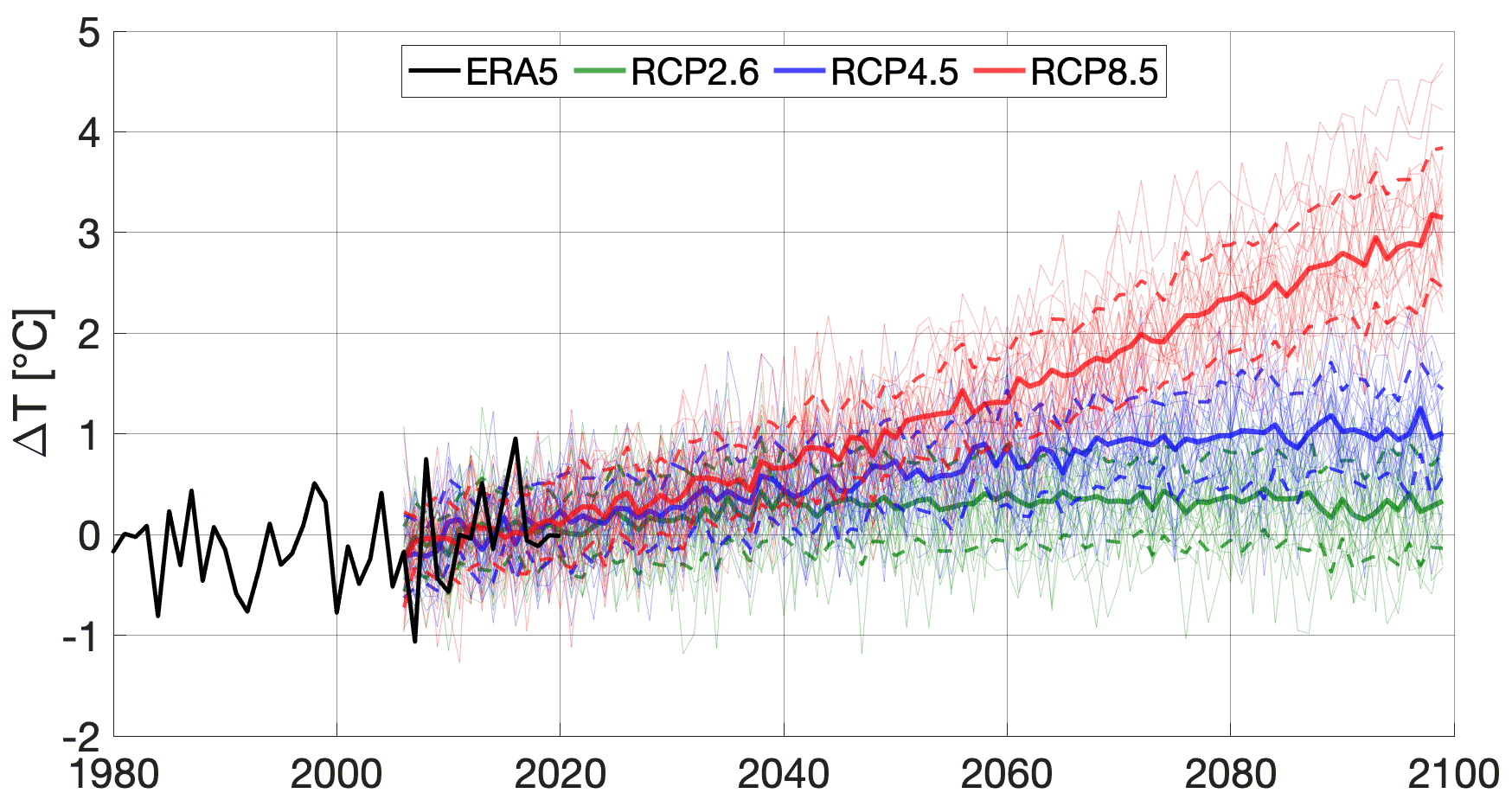
Figure 4Temperature projections for the Mocho-Choshuenco ice cap through the 21st century for three different scenarios, RCP2.6, RCP4.5, and RCP8.5, along with historical ERA5 data which are used for the transient spin-up. The thin lines show projections of the 23 individual climate models, thick solid lines indicate their mean, and thick dashed lines indicate the 1σ confidence interval. The period between 2006 and 2020 is used as the reference period for each individual model.
ERA5 is a state-of-the-art global reanalysis produced by the European Centre for Medium-Range Weather Forecasts (ECMWF). It combines large amounts of historical observations into global estimates using advanced modelling systems and data assimilation, i.e. Integrated Forecasting System (Cycle 41r2) (Hersbach et al., 2020). ERA5 has a spatial resolution of (∼30 km) and vertical resolution of 137 levels from the surface to a height of 80 km.
Given that there are no available long-term surface meteorological data around the ice cap, we contrasted 700 hPa ERA5 temperature data against the radiosonde data (Integrated Global Radiosonde Archive v2, available at https://www1.ncdc.noaa.gov/pub/data/igra/, last access: 11 February 2021) from Puerto Montt (41.5∘ S, 72.9∘ W) for the period 1979–2019. This is due to the fact that Schaefer et al. (2017) found a very good correlation between the 700 hPa pressure level temperature from the radiosonde data at Puerto Montt and temperature measured at the Mocho automatic weather station. In this respect, ERA5 shows reasonable skills in capturing the long-term regional temperature trend ( in 41 years) detected in the radiosonde data ( in 41 years) with a high temporal correlation (0.77).
Due to this temperature increase of around 0.2 ∘C, we build the steady state by lowering the mean ELA (BELA) by 18 m in 1979 with respect to the state in 2013, according to the ELA-temperature gradient of 88 m K−1 which we determine in Sect. 2.6. Afterwards, we adjust the model parameters mean ELA (BELA), ELA amplitude (AELA), maximum SMB (S0), SMB gradient (M0), direction of maximum ELA (φ0), and sliding coefficient (Cb) in order to match the present-day observations of SMB, ice thickness, ice extent, ice volume, and surface velocity of the ice cap. While the parameters defining the SMB parameterization were calibrated under observational constraints, Cb was purely used as a calibration parameter. We discuss this in more detail in Sect. 4.1. It is important to note that the steady-state spin-up in the 1970s is a theoretical construct as the glacier had been losing mass before this period and was not in a steady state. It is only to be interpreted as a first step in order to get an accurate representation of the shrinking ice cap in 2013 with its negative SMB.
2.5 Temperature projections
The main goal of this study is to project the future evolution of the Mocho-Choshuenco ice cap. We use future temperature simulations from 23 climate models participating in CMIP5 (see Appendix A). To ease the calculations, all the models were interpolated onto a common grid of using bilinear interpolation. Then the time series of each model were extracted from the grid point corresponding to Mocho-Choshuenco ice cap (40∘ S, 72∘ W). As the model trajectories start in 2006 and in order to be consistent with the reference ice cap conditions based on the observational dataset obtained between 2009 and 2013, we used the period from 2006 to 2020 as the reference period rather than the commonly used historical periods (e.g. 1976–2005) in order to construct projections of temperature anomalies. For each of the individual models, the mean temperature between 2006 and 2020 was then subtracted from the whole time series, leading to anomaly temperature projections with respect to this period. At the final step, the SICOPOLIS model was driven by each of the 23 model projections to provide a more robust assessment of the future evolution of the Mocho-Choshuenco ice cap. This allows us to assess the uncertainty associated with climate model differences. In addition to the future projections, we also include a control run in our analysis in which we run the model for the period 2013–2100 with zero temperature anomaly with respect to the reference period 2006–2020. This enables us to calculate a committed mass loss and assess the influence of ice dynamics alone, independent of future temperature increase.
Our approach makes use of three emission scenarios following the IPCC protocols (IPCC, 2013): high-mitigation, Paris Agreement compatible (RCP2.6); medium stabilization scenario with a peak around 2040, then decline (RCP4.5); and high-end baseline scenario with no control policies of greenhouse gas emissions (RCP8.5). This allows us to contrast the future evolution of the Mocho-Choshuenco ice cap under different emission scenarios, together with the uncertainty introduced by future emissions. Figure 4 shows the projected changes in temperature obtained from 23 individual climate models for the ice cap under the three different emission scenarios until the end of the century. This yields 69 projections which are all used to run SICOPOLIS and are averaged afterwards. All projections follow a similar trend until the 2040s, when the RCP8.5 scenario separates from the others and continues to increase throughout the century, leading to a model mean temperature increase of 3.15±0.69 ∘C by the end of the century. The temperature projections under the RCP2.6 and RCP4.5 scenarios have largely similar evolutions after the 2050s with weaker projected changes than those in RCP8.5. By the end of the century, projected temperature increases for the RCP2.6 and RCP4.5 scenarios are 0.33±0.47 and 1.01±0.43 ∘C, respectively.
2.6 Glacier sensitivity to temperature change
To link the projected 21st-century temperature rise to ice dynamics, it is necessary to relate the temperature anomalies to changes in SMB, which is determined by the mean ELA (BELA) in our case. We assume that temperature is the only influencing factor on the projected net SMB without explicitly distinguishing between precipitation and runoff. Further, we focus on annual rather than melt-season temperature projections as the climate models project both to be very close to each other in the Mocho-Choshuenco volcanic complex. There are 4 years (2009–2013) when both the ELA and annual mean temperature at a similar altitude are available (Schaefer et al., 2017). These data are shown in Fig. 5, together with the ELA error estimates.
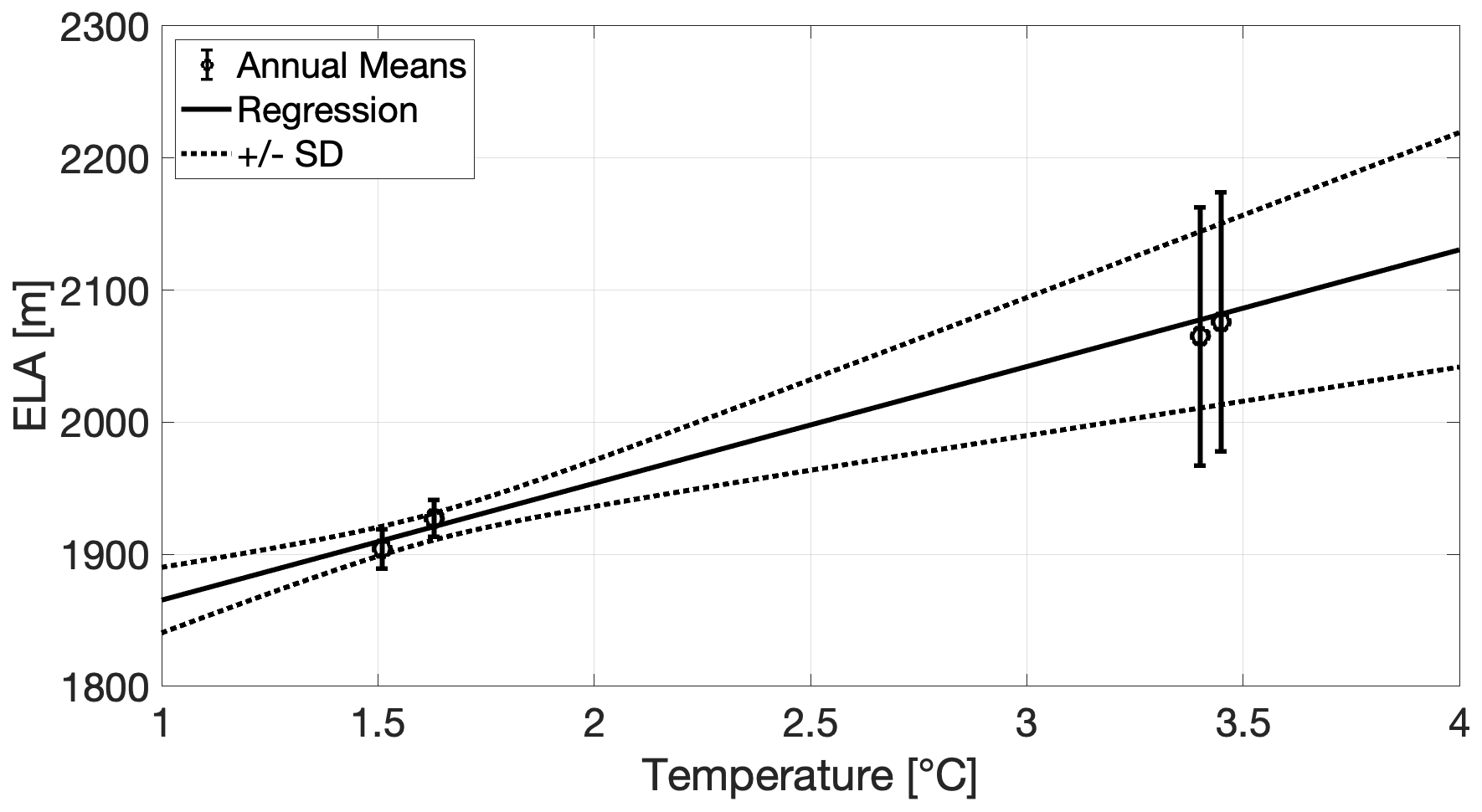
Figure 5Relationship between annual temperature and ELA on Mocho-Choshuenco ice cap. The error bars indicate the error as estimated by Schaefer et al. (2017). The relationship between ELA and temperature was found through weighted linear regression.
In order to predict the ELA for any temperature, we first assume a linear relationship between both and solve a weighted least squares problem to find the slope and intercept (i.e. ELA gradient and ELA for 0 ∘C). ELA predictions for any temperature can be made by multiplying the forward operator with the vector m containing both model parameters:
where m is distributed according to a bivariate normal distribution 𝒩(μ,Σ) with mean vector μ and model covariance matrix Σ (e.g. Aster et al., 2018):
Inserting the observed data, we identify the forward operator , the data covariance matrix Σd, and the vector of observed ELAs as
Predictions for a general temperature T can be made through
with
where is our estimated increase in ELA per degree Celsius, and μ2=1777 m is the ELA that we would obtain for a yearly average temperature of 0 ∘C. Figure 5 shows the mean of ELA predictions against temperature, together with the 1σ confidence interval.
Since the temperature projections give anomalies with respect to the period 2006–2020, we only rely on relative rather than absolute temperatures. Therefore, we convert the temperature changes into changes of ELA with the parameter , which means that the ELA increases by 88 m per ∘C temperature increase. We assess the uncertainty propagation of this parameterization through the ice flow simulation code by performing additional experiments with upper and lower ELA gradients , which corresponds to the 1σ confidence interval.
3.1 Spin-up and model calibration
Following the spin-up and calibration procedure explained in Sect. 2.4, we tune the model to find the following optimal parameters: BELA=2050 m, AELA=87.5 m, and , , and . We discuss the physical plausibility of these values in Sect. 4.1.
The spin-up is evaluated against observations in Fig. 6. Figure 6a shows the thickness distribution and extent of the simulated ice cap. The model captures the general outlines of the ice cap with only small inaccuracies at some outlet tongues. In Fig. 6b, we compare the simulated and observed ice thickness. Overall, the simulations overestimate ice thickness in the northern part of the ice cap and underestimate it in the south-east. Figure 6c shows that the simulated ice thickness is in reasonable agreement with observations along the radar profiles, with a high correlation (0.91), and the root mean square error (RMSE) that is around 13 % of the maximum measured ice thickness.
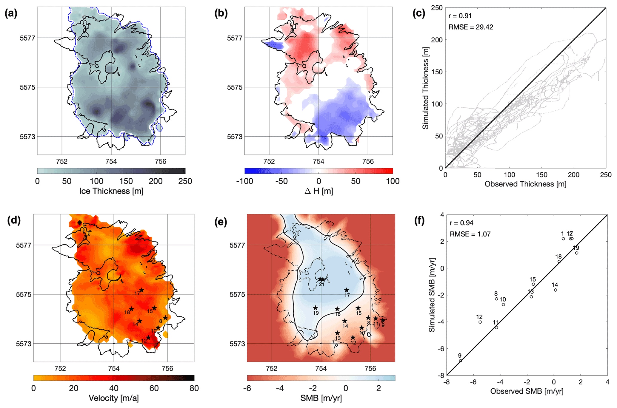
Figure 6Results of the transient spin-up for 2013. (a) Ice thickness distribution with observed (black) and modelled (blue) extent, (b) difference between modelled and observed ice thickness, (c) modelled thickness against observed thickness along radar profiles, (d) surface flow velocity and stakes with velocity observations, (e) modelled surface mass balance over model domain with SMB stakes as black stars and simulated ELA as solid black line, and (f) modelled SMB against observed SMB at stakes.
The velocity map in Fig. 6d shows velocities of less than 50 m yr−1 on most parts of the ice cap, matching well with the observed low velocities that were measured in spring 2013 (Geoestudios, 2013). Stakes where velocity measurements are available are marked with black stars in Fig. 6d. Observed and modelled velocities at these locations are compared in Table 1, showing an overall good agreement (RMSE of 12.5 m yr−1), with simulated velocities being on average 9.4 m yr−1 lower. However, the modelled velocities represent a yearly average, whereas the velocity measurements were taken in the spring season, making a direct comparison difficult, and these values should only be seen as a rough orientation.
The simulated SMB in Fig. 6e matches well with observations reported by Schaefer et al. (2017) with the observed SMB distribution, SMB gradient, and ELA on the south-eastern catchment. Figure 6f shows a direct comparison of modelled SMB at the stake locations and the respective observations. The fit is very good, with a high correlation (0.94), and the RMSE corresponds to roughly 11 % of the absolute range between highest and lowest observed SMB.
3.2 Projected future evolution of the ice cap
The evolution of the total ice volume under the RCP2.6, RCP4.5, and RCP8.5 scenarios, as well as the control run with a zero-anomaly with respect to the reference period 2006–2020, is shown in Fig. 7. For the control run, the ice cap loses 28 % of its volume by 2100, which can be interpreted as the committed loss due to the non-steady-state conditions during the reference period. The projections for the 23 individual climate models (thin lines) can be summarized by the multimodel ensemble mean (thick solid lines) and 1σ confidence interval (thick dashed lines). All three scenarios start with a negative slope and lose mass at a similar rate, reflecting the present-day negative SMB. From the 2050s, the scenarios begin to diverge significantly, indicating that the differences between temperature increases of each projection start to dominate the ice dynamics. By the end of the century, all mean curves flatten out.
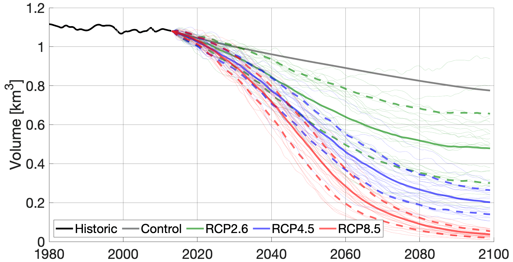
Figure 7Ice volume evolution under the three scenarios RCP2.6 (green), RCP4.5 (blue), and RCP8.5 (red) until the year 2100. Thin lines show the 23 individual evolutions from different climate models, thick solid lines indicate their mean, and thick dashed lines indicate the mean plus and minus the standard deviation. The solid black line shows the evolution of the transient spin-up between 1979 and 2013, and the thick grey line shows a control run based on a zero-anomaly with respect to the reference period 2006–2020.
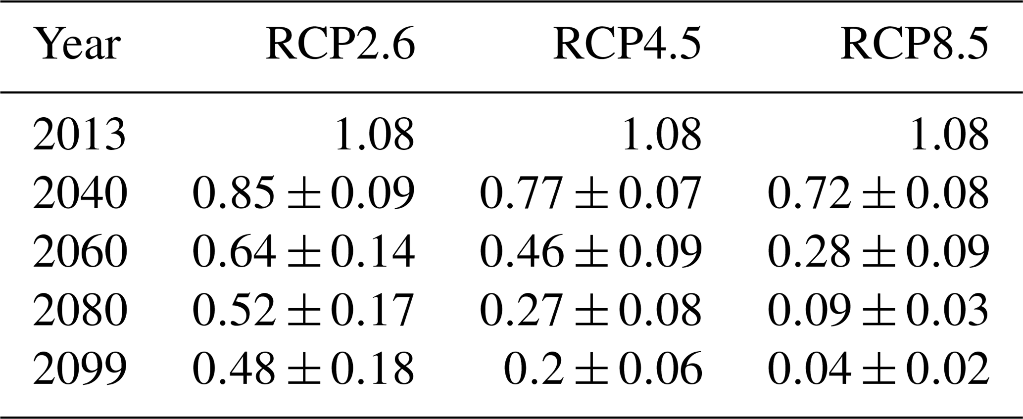
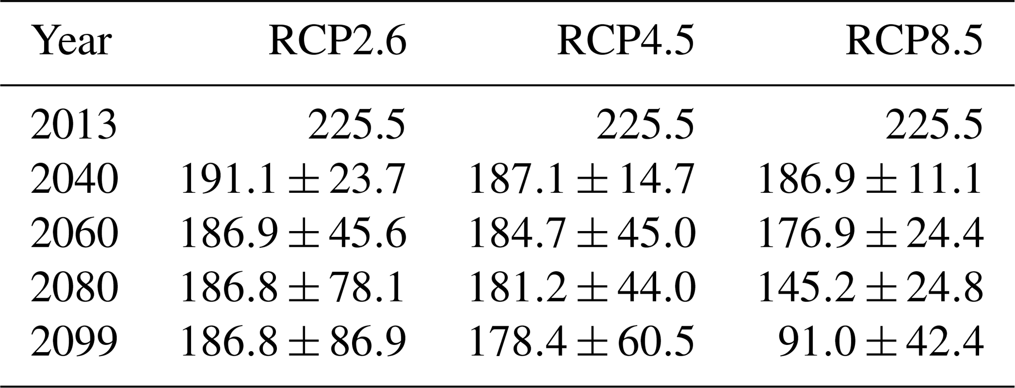
In terms of variability between the climate models, the RCP2.6 scenario starts with a narrow confidence interval which gets larger throughout the century, reflecting disagreements between the ensemble members. For the RCP4.5 scenario, this is only the case until the 2060s, and as the mean curve flattens, the uncertainties remain constant. The uncertainty of the RCP8.5 scenario increases until the 2050s and then decreases until the year 2100. These contrasts in the projections under different emission scenarios reflect the higher signal-to-noise ratio for the RCP8.5 scenario as this scenario has a more prominent temperature increase (also see Fig. 4). Projected ice volumes and uncertainties for different scenarios and years are summarized in Table 2.
Table 2Projected ice volumes in cubic metres for different scenarios and years: mean and standard deviation obtained by forcing SICOPOLIS for 23 climate models.
In addition to the uncertainty introduced by different climate models, we analyse the impact that the ELA dependence on temperature has on glacier projections. We average the 23 climate model temperature projections for the three scenarios before running SICOPOLIS instead of forcing it individually with each climate model as in the previous sections. With these mean projections, we perform three model runs for each scenario: the mean gradient between temperature and ELA (88 m K−1) and the upper and lower bound of the 1σ confidence interval (51 and 125 m K−1). The resulting ice volume evolutions are shown in Fig. 8. The mean curves are very similar to those obtained in Fig. 7; however, the spread is higher for the RCP4.5 and RCP8.5 scenarios and lower for the RCP2.6 scenario with respect to those obtained in Fig. 7.
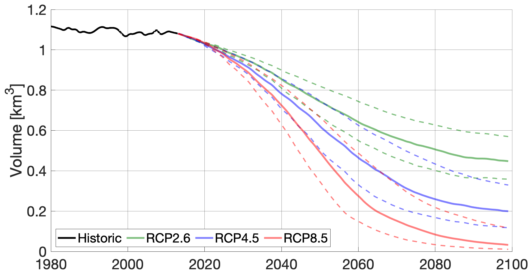
Figure 8Volume evolution for different gradients between ELA and temperature, with the mean shown in solid lines and the 1σ confidence interval indicated by dashed lines.
The ice volume loss can be broken down into thinning and retreat, i.e. to a lower ice thickness and a smaller ice area, respectively, towards the end of the century. Figure 9 shows the evolution of the ice thickness distribution for the different scenarios obtained after averaging over all 23 climate models for each of the three scenarios, and Table 3 gives an estimate of thinning by displaying the maximum ice thickness in the same years obtained after averaging over all 23 climate models.
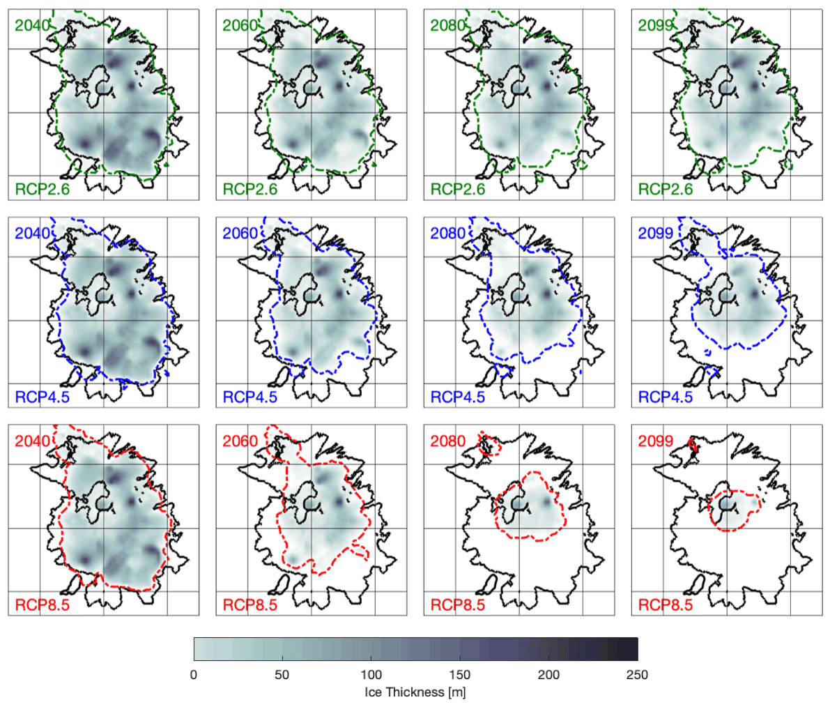
Figure 9Ensemble mean ice thickness for three different future temperature scenarios and four different years obtained by averaging the thickness obtained from all 23 climate models in every grid cell. The dashed coloured lines show modelled ice extent, and solid black lines show the observed ice extent in 2013.
Table 3 Projected maximum ice thickness in metres for different scenarios and years: mean and standard deviation obtained by forcing SICOPOLIS for 23 climate models.
In the RCP2.6 scenario, thinning is dominant until the year 2060, and especially a dramatically reduced maximum ice thickness is evident by 2040 (see Table 3). After 2060, ice loss becomes less drastic, and thinning rates are relatively low until 2100. Retreat is overall moderate and mostly exists in the south-east between 2060 and 2080, presumably as a dynamic response to thinning in the previous decades.
The RCP4.5 scenario shows a stronger retreat pattern compared to the RCP2.6 scenario throughout the century, mostly until 2080. This retreat is accompanied by strong thinning before 2080, and afterwards the reduction in ice thickness is less pronounced.
The high-end scenario (RCP8.5) shows a clearly different pattern in both thinning and retreat over the 21st century. While the thickness pattern for 2040 is comparable to the two other scenarios, ice loss clearly accelerates between 2040 and 2080. This can be discerned by the faint colours in the last two plots indicating an ice thickness of mostly under 100 m and a dramatic retreat until the year 2099 (see also Table 3).
4.1 Present-day simulations
The first part of our study consists of the creation of a present-day steady state of the Mocho-Choshuenco ice cap. Since drivers of the SMB such as solar radiation and snow redistribution are strongly aspect-dependent, we developed a new SMB parameterization accounting for aspect-dependent SMB variations (see Sect. 2.3). The values of the SMB parameterization were tuned within realistic ranges to find an optimal configuration that reproduces present-day observations of ice thickness, ice extent, SMB, and surface velocity. Here we discuss the physical plausibility of the six tuning parameters. The SMB gradient was obtained to match the variation of observed SMB at stakes with respect to the elevations, giving a very good match (see Fig. 6e and f). The direction of maximum ELA () was chosen based on the fact that the north-western part is generally more exposed to both solar radiation and snow erosion by wind and consequently less melt (more shade) and more accumulation due to snow drift on the south-eastern part. The maximum SMB () was maintained in a range that keeps the stakes at the highest elevations close to the observed values and fine-tuned in the calibration process. Mean ELA and ELA amplitude (BELA=2050 m, AELA=87.5 m) were varied in order to match observations and constrained to maintain a similar ELA in the south-eastern part as observed by Schaefer et al. (2017). This is given with an ELA of 1963 m in our model, which is near the mean value of 1993 m obtained from measurements between 2009 and 2013 (Schaefer et al., 2017). As no direct observations of the basal conditions on the ice cap are available, the sliding parameter () was purely used as a tuning parameter to match the observations, but its value is within the typical range.
The ice thickness map in Fig. 6a reveals that we are able to reproduce the general magnitude of ice thickness well (mostly around 100–150 m, with a maximum value of up to 250 m). The ice extent is well reproduced, as a comparison between the black and blue lines shows. At the margins, some ice tongues are not recovered, and some others are added. Most notably, this is the case for one of the south-western ice tongues where stakes B9 and B11 are located. This is a minor inconsistency in our model, and due to our simplified parameterization it would be impossible to recover all details of the observations on the ice cap.
Figure 6b shows the difference in ice thickness between our model and the interpolated ice thickness map in Fig. 2a. Ice thickness is mostly underestimated in the south-east and overestimated in the north. However, as Fig. 2a shows, there are in fact very few radar measurements especially in the north, and therefore a direct comparison with the interpolation is not meaningful in many places. A more valuable comparison is that in Fig. 6c, showing how our model reproduces the directly measured ice thickness along the radar tracks. It shows a satisfying correlation between both with a low RMSE, and most of the simulated thickness values are close to the observed ones. In general, we mostly overestimate the ice thickness in thin areas and underestimate it where ice cover is thick. This might indicate local inaccuracies introduced by our choice of the SIA as a low-order ice flow parameterization, but overall ice thickness is well reproduced.
Modelled ice velocities at the surface are low on the flat parts of the ice cap and get higher towards the outlets of the ice cap (Fig. 6d). The simulated velocities at the stake locations are generally lower than the observed ones (Table 1). However, this comparison has to be interpreted with some care as the observed values were taken in October, while the simulated velocities are representative of the whole year. Furthermore, the flow exponent n=3 in Glen's flow law leads to a significant underestimation of surface velocities where thickness is also underestimated. Most stakes lie in areas where the ice is thinner in simulations than in observations (see Fig. 6b and d), making this a reasonable explanation. On several stakes (B10 and B15), the velocities are well matched, and we conclude that our spin-up reproduces the observed ice cap well considering the given observations.
Figure 6e shows the modelled SMB distribution on the ice cap. The only observations available are on the south-eastern catchment, and the distribution of SMB compares well to that of previous observations (see Fig. 9a in Schaefer et al., 2017). Also, simulated and observed SMB values at individual stakes match well, as depicted in Fig. 6f. Most of the modelled values are very close to the observations, with an RMSE of around and a high correlation. As SMB controls the ice evolution in our future projections, these SMB comparisons indicate that our projections are realistic within the observational limitations.
In terms of our choice for a transient spin-up with temperature forcing over the last 35 years, there are several factors that indicate its superiority over a steady-state spin-up in which the present-day glacier is built under a constant climate. Most importantly, currently observed SMB is negative (Schaefer et al., 2017), indicating a shrinking ice cap which by definition could not be reproduced by a steady state. Our choice of a 35-year transition period is justified by the turnover time of the ice cap, which we calculated as 27 years (see Sect. 2.4). While we do not reproduce the exact glacier state in previous decades, the calculated times indicate that the most important features of the transient state in 2013 should be captured by our model. The control run under a constant 2006–2020 mean temperature in Fig. 7 still shows a remarkable shrinking of the ice cap in 2100 compared to the most optimistic scenario. This indicates that committed mass loss plays a significant role in future glacier evolution which could not be represented by a steady-state spin-up. A recent study found highly accelerated glacier mass losses worldwide in the last two decades (Hugonnet et al., 2021), underpinning the need for a transient model initialization and showing that our projected high mass loss rates in the upcoming decades seem to be more realistic than the more moderate ones that would be obtained after a steady-state model initialization.
4.2 21st-century projections
In all scenarios, the future projections start with a significant negative trend due to the negative present-day SMB. Afterwards, the different scenarios diverge, and in this section we interpret their evolution based on the results presented in Sect. 3.2.
The effect of emission reduction in the RCP2.6 scenario starts to appear around 2050, which correlates well with an estimated response time of 37 years for our ice cap. From the 2050s, ice loss starts to be less drastic for this scenario, and towards the end of the century, the ice cap seems to stabilize at about half its present-day volume. Thinning is more dominant than retreat until 2060, and afterwards retreat takes over, presumably as a dynamic response to the previous thinning.
The uncertainties associated with the volume projections are particularly high for the RCP2.6 scenario, with a large spread introduced by the different climate models. Therefore, we conclude that it is essential to perform ice cap projections with an ensemble of climate models rather than a single model in order to avoid bias towards the underlying assumptions of one particular model.
The RCP4.5 scenario assumes a significant reduction of emissions only after the 2040s, and this is reflected in our results by the fact that ice volume steadily decreases until around 2080 and only then becomes more stable. Apart from the reduced emissions, another explanation for the flattening of the curve is the fact that by 2080 most of the plateau of the ice cap will have melted away, and further elevations of ELA have less influence due to the steep slopes around the summits. This interpretation is confirmed by the ensemble uncertainty, indicating a generally good agreement between the climate models with regards to the state of the ice cap at the end of the century. As opposed to the RCP2.6 scenario, retreat sets in earlier and accompanies the thinning that is prevalent during the whole 21st century.
In the RCP8.5 scenario, assuming no emission reduction at all, the ice volume loss becomes much steeper from the 2030s, losing quickly most of the mass of the ice cap. This mass loss is driven by both high retreat and thinning rates. Only after 2080, with around 10 % of the initial ice volume left, do losses start to become less when the ELA retreats towards the summit. By the year 2100, the only remaining patches of ice are very close to Mocho's summit. The ensemble uncertainty for this scenario is highest during the extreme volume loss in the middle of the century, and it becomes very small towards the end of the century, indicating that most climate models agree on the almost complete disappearance of the ice cap.
4.3 Limitations of our approach
In this study, the principal uncertainties we assign to our results are based on the spread of the temperature projections of the global climate models and on the uncertainty of the temperature–ELA parameterization. In this section, we discuss possible further sources of uncertainty and make suggestions on how future work could encounter these challenges.
Our approach is based on the shallow-ice approximation (SIA), with assumptions including almost parallel and horizontal glacier bed and surface, significantly larger horizontal than vertical dimensions, and simple-shear ice deformation. While these assumptions hold well for the large Greenlandic and Antarctic ice sheets, it is less obvious that the SIA can be employed on such a small study object as the Mocho-Choshuenco ice cap. The SIA assumptions are violated especially in the steep regions around the two summits and towards the boundaries of the present-day ice cap. However, they hold true for large parts of the plateau which is the most important area in our future projections. Previous studies have suggested that low-order assumptions such as the SIA hold well for glaciers whose behaviours are mostly driven by SMB (Adhikari and Marshall, 2013), which is the case for the Mocho-Choshuenco ice cap. However, it would be a valuable experiment to reproduce our results with a full-Stokes model such as Elmer/Ice to verify the applicability of the SIA.
Knowledge about the bed of the ice cap is essential to perform ice flow simulations. We created a bed map based on present-day topography and a number of ground-penetrating radar profiles published by Geoestudios (2014). Even though these profiles cover a significant portion of the ice cap, there are large gaps in data coverage, especially in the north-western part of the ice cap. More observations could help to reduce the uncertainty introduced by these gaps.
Regarding the ELA gradient we use to relate temperature increase to glacier SMB, it is important to note that we have only a few data points given for this relationship (Schaefer et al., 2017). With more years of ELA–temperature pairs and a thorough uncertainty estimation, we could achieve a higher confidence in our ELA gradient. However, by performing the simulations for the mean gradient and a lower and upper bound, we are within the range of most previous studies (e.g. Six and Vincent, 2014; Sagredo et al., 2014; Wang et al., 2019).
Another significant limitation lies in the SMB parameterization. While the new aspect-dependent parameterization was able to improve the reproduction of the present-day ice cap significantly, there is still space for improvement. Especially the northern part is still not well reproduced by SICOPOLIS, and it might be advantageous to extend the new parameterization to the Choshuenco peak. In order to verify our parameterization, it would be helpful to obtain SMB measurements in the north-west, i.e. between both summits, and thus extend the stake network that is currently focused on the main catchment in the south-east of Mocho's summit. This could provide more observational constraints on the ELA difference between the north-west and south-east.
Another way of producing more realistic SMB maps for the ice cap would be using explicit models that try to quantify the physical processes which determine glacier mass balance, e.g. the COSIPY model (Sauter et al., 2020). A drawback of these complex models is that they need many input parameters (such as precipitation, relative humidity, or wind speed) with a high spatial resolution. These can be obtained by regional climate model simulations (e.g. Bozkurt et al., 2019). However considerable uncertainties are associated with these simulations, and a careful validation of the results is necessary before using them as drivers of SMB simulations. Additionally, only a few high-resolution regional climate simulations are available at the moment which is why we prefer our simple temperature-dependent SMB parameterization combined with a multi-model approach using 23 different GCMs as drivers of our simulations.
4.4 Global context of glacier decline
To our knowledge, there are only a few previous studies that have projected the future evolution of glaciers in the Andes. The nearest study object to the Mocho-Choshuenco ice cap is the Northern Patagonian Ice Field for which by 2100 an ice mass loss of 592 Gt has been projected under the A1B scenario which is comparable to the RCP6.0 scenario and therefore between our results for RCP4.5 and RCP8.5 (Schaefer et al., 2013). Relating this ice loss to more recent estimates of total ice mass (Carrivick et al., 2016; Millan et al., 2019), around 50 % of the ice mass is projected to disappear. However, these simulations were performed on a fixed geometry, and they therefore considered only changes in SMB, making it difficult to compare their results to ours. Collao-Barrios et al. (2018) obtained a committed mass loss of approximately 10 % for San Rafael Glacier under the current climate, significantly less than the 28 % which we estimated. However, they maintained a constant glacier area during their simulations and therefore neglected glacier retreat, which could dramatically change rates of frontal ablation.
Möller and Schneider (2010) projected the future evolution of Glaciar Noroeste, an outlet glacier of the Gran Campo Nevado ice cap in southern Patagonia between 1984 and 2100. Their projections were made for the B1 scenario and yielded a volume loss of around 45 %, which is significantly less than the 61 % volume loss that we project for the comparable RCP4.5 scenario between 2013 and 2100. Their results are based on a calibrated relationship between area and volume and not on ice flow modelling as in our study.
Hock et al. (2019) and Marzeion et al. (2020) are two studies which projected 21st-century glacier evolution worldwide using 6 and 11 different glacier models, respectively. In both studies, the southern Andes are one of the study areas, and they both predict rather low mass losses of around 20 % for the RCP2.6 scenario and under 50 % for the RCP8.5 scenario, which is considerably less than ours (55 % for RCP2.6, 97 % for RCP8.5). However, making a direct comparison between these studies and our results is problematic for several reasons. First, their study region is highly dominated by the large Patagonian ice fields, where many glaciers terminate in the ocean or lakes, with frontal ablation contributing to 34 % of overall mass loss (Minowa et al., 2021). Frontal ablation, however, is only parameterized in 1 of 6 (Hock et al., 2019) and 2 of 11 models (Marzeion et al., 2020), and their results therefore need to be interpreted with care. Second, SMB in these global models is highly simplified and averaged over a huge amount of glaciers. While this is convenient in obtaining satisfactory global projections, the accuracy is likely limited on a regional or local scale. In fact, SMB is positive on the Southern Patagonian Ice Field (Schaefer et al., 2015), reinforcing the need to account for frontal ablation when estimating mass losses. In the case of our small ice cap, many detailed SMB observations are available, and our results therefore yield valuable local-scale estimates of SMB and future mass loss against which global models such as those in Hock et al. (2019) and Marzeion et al. (2020) can be calibrated.
The only glacier in the Andes for which future projections under climate change scenarios are available, based on simulations with an ice-flow model (Elmer/Ice), is Zongo Glacier in Bolivia by Réveillet et al. (2015). They projected 40 % and 89 % volume losses for the RCP2.6 and RCP8.5 scenarios, respectively. The value for the high-end scenario is comparable to ours (97 %), which might be expected as both glaciers are going to disappear by the end of the century and therefore have already lost the majority of their ice mass relative to their present state. Our projections for RCP2.6 (55±16 %) are also within the range of their RCP2.6 projections. However, this comparison needs to be treated with care due to the climate differences between the tropics and the Wet Andes and also due to the higher ELA gradient with temperature of 150 m K−1 used in their study in comparison to 88 m K−1 used in our study. Another factor that changes from glacier to glacier is the geometric conditions which can have a significant impact on volume losses.
Outside the Andes, only a few studies have projected glacier evolution in the 21st century with ice flow models. Among them is that of Adhikari and Marshall (2013) who performed ice flow simulations on Haig Glacier in the Rocky Mountains and projected the disappearance of the glacier by 2080 under the RCP4.5 and RCP8.5 scenarios. In Europe, Jouvet et al. (2011) projected a volume loss of 90 % for Grosser Aletschgletscher in Switzerland by 2100 under the A1B scenario and indicated that even under the present climate the glacier is in disequilibrium and would continue to lose significant amounts of ice. Wang et al. (2019) investigated the future evolution of Austre Lovénbreen with the full-Stokes ice flow model Elmer/Ice, a mountain glacier in Svalbard, and found that with an intermediate temperature increase scenario the glacier would disappear by 2120 and by 2093 for the most pessimistic scenario.
Even though different model set-ups and parameterizations were applied for all glaciers in the mentioned studies, most of them show a similar trajectory for the glacier evolution in the next 60 to 100 years, and our projections for the Mocho-Choshuenco ice cap fit well into them. All of them lose a high percentage of ice mass during the 21st century, and we can expect many mountain glaciers in different parts of the world to disappear in the first half of the 22nd century without reductions of greenhouse gases.
In this study, we applied the ice-sheet model SICOPOLIS to reproduce the current state of the Mocho-Choshuenco ice cap and to project its future evolution under different emission scenarios. To our knowledge, this is the first estimate of future glacier evolution obtained from an ice flow model forced with climate change scenarios for the Wet Andes and the second for the whole Andes. Using a linear temperature–ELA parameterization, we investigate the future of the ice cap using projected temperature changes from 23 GCMs as input. A considerable spread of the projected ice volume at the end of the 21st century is obtained, depending on the emission scenario and GCM.
The mean projected ice volume losses by the end of the century are 56±16 % (RCP2.6), 81±6 % (RCP4.5), and 97±2 % (RCP8.5) with respect to the ice volume derived from measurements in 2013. This means that even under the most optimistic emission scenario the expected loss of ice volume is between 40 % and 72 %. The spread between the results, when driving the model by different GCMs, becomes lower when considering higher emission scenarios: under the emission scenario RCP8.5, which does not consider a reduction in our emission of greenhouse gases, it is likely that the ice cap will lose more than 95 % of its current volume by 2100. Since temperature projections are relatively uniform in the region and geometry of the surrounding ice caps are similar to Mocho-Choshuenco ice cap, we can expect similar projections of high volume losses for other ice caps in the Chilean Lake District (39–41.5∘ S). The Mocho-Choshuenco ice cap is the smallest ice body to which SICOPOLIS has been applied so far, justified a priori by the cap-like geometry (as opposed to, for example, valley glaciers) and a posteriori by the reasonably good performance of the model in replicating the present-day ice cap. Nevertheless, it would be valuable to check if the application of a full-Stokes glacier flow model (as, for example, Elmer/Ice; Gagliardini et al., 2013) affected the simulated state of the ice cap notably or if the disagreements are mainly caused by our simplified SMB parameterization.
When trying to project the future of the largest ice bodies of the Wet Andes (the Patagonian ice fields), the interaction of their outlet glaciers with the surrounding water bodies becomes crucial. Adequate parameterizations for frontal ablation are necessary, which allow the glaciers to adapt their frontal positions according to the glacier flow, which, in turn, will be crucially determined by its interaction with the water bodies.
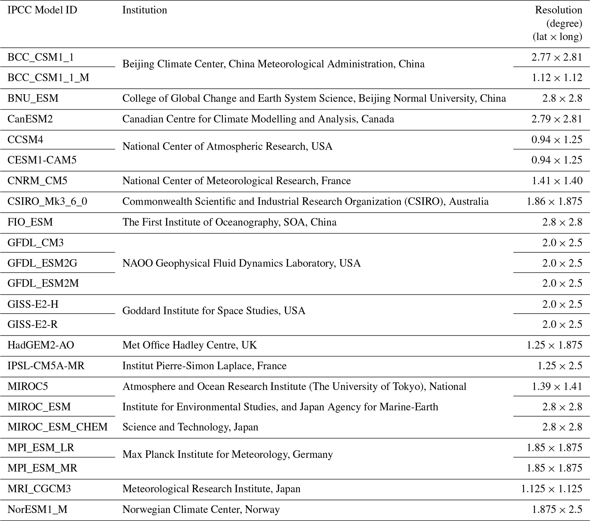
Table A1 gives details on the 23 global climate models that were used to force SICOPOLIS with future temperature projections.
Table A1Details of global climate models used in this study. For further information on CMIP5 and the individual models, see Taylor et al. (2012) and references therein.
SICOPOLIS is free and open-source software, available through a persistent Git repository hosted by the Alfred Wegener Institute for Polar and Marine Research (AWI) in Bremerhaven, Germany (https://gitlab.awi.de/sicopolis/sicopolis, Greve and SICOPOLIS Developer Team, 2021). Detailed instructions for obtaining and compiling the code are at http://www.sicopolis.net (last access: 3 August 2021). The output data produced for this study are available at Zenodo, https://doi.org/10.5281/zenodo.5053396 (Scheiter et al., 2021).
MarS, RG, and MatS designed the study. RG developed the ice-sheet model SICOPOLIS. MatS ran the simulations with advice from MarS and RG. EF contributed to the simulations. DB provided the temperature projection data and assisted with the ice cap projections. MatS wrote the manuscript with contributions from all authors. All authors discussed and interpreted the results.
The authors declare that no competing interests are present.
Publisher's note: Copernicus Publications remains neutral with regard to jurisdictional claims in published maps and institutional affiliations.
We are grateful to Gino Casassa for providing the ice thickness data used in this study. Discussions with Andrew Valentine, Buse Turunçtur, and Shubham Agrawal helped to improve this paper. We thank Klaus Spitzer and Malcolm Sambridge for their generous support in undertaking this research. We acknowledge the World Climate Research Programme Working Group on Coupled Modelling, which is responsible for CMIP, and we thank the climate modelling groups (listed in Table A1) for producing and making available their model output. We thank the editor Benjamin Smith for handling the manuscript and two anonymous referees whose comments helped to improve the quality of the manuscript.
Matthias Scheiter acknowledges financial support from the Australian National University and the CSIRO Deep Earth Imaging Future Science Platform. Marius Schaefer is supported by the FONDECYT Regular Grant, Etapa 2018, grant no. 1180785. Eduardo Flández acknowledges support from FONDECYT grant no. 1201967 and a doctoral fellowship from ANID. Deniz Bozkurt acknowledges support from CONICYT-PAI 77190080, ANID-PIA-Anillo INACH ACT192057, and ANID-FONDECYT-11200101. Ralf Greve was supported by the Japan Society for the Promotion of Science (JSPS) KAKENHI grant nos. JP16H02224, JP17H06104, and JP17H06323, by a leadership research grant of Hokkaido University's Institute of Low Temperature Science (ILTS), and by the Arctic Challenge for Sustainability projects ArCS and ArCS II of the Japanese Ministry of Education, Culture, Sports, Science and Technology (MEXT) (programme grant numbers JPMXD1300000000 and JPMXD1420318865).
This paper was edited by Benjamin Smith and reviewed by two anonymous referees.
Adhikari, S. and Marshall, S. J.: Influence of high-order mechanics on simulation of glacier response to climate change: insights from Haig Glacier, Canadian Rocky Mountains, The Cryosphere, 7, 1527–1541, https://doi.org/10.5194/tc-7-1527-2013, 2013. a, b
Aster, R. C., Borchers, B., and Thurber, C. H.: Parameter estimation and inverse problems, Elsevier, Amsterdam, the Netherlands, 2018. a
Bernales, J., Rogozhina, I., Greve, R., and Thomas, M.: Comparison of hybrid schemes for the combination of shallow approximations in numerical simulations of the Antarctic Ice Sheet, The Cryosphere, 11, 247–265, https://doi.org/10.5194/tc-11-247-2017, 2017. a
Blatter, H. and Greve, R.: Comparison and verification of enthalpy schemes for polythermal glaciers and ice sheets with a one-dimensional model, Polar Sci., 9, 196–207, https://doi.org/10.1016/j.polar.2015.04.001, 2015. a
Bozkurt, D., Rojas, M., Boisier, J. P., Rondanelli, R., Garreaud, R., and Gallardo, L.: Dynamical downscaling over the complex terrain of southwest South America: present climate conditions and added value analysis, Clim. Dynam., 53, 6745–6767, https://doi.org/10.1007/s00382-019-04959-y, 2019. a
Braun, M. H., Malz, P., Sommer, C., Farías-Barahona, D., Sauter, T., Casassa, G., Soruco, A., Skvarca, P., and Seehaus, T. C.: Constraining glacier elevation and mass changes in South America, Nat. Clim. Change, 9, 130–136, https://doi.org/10.1038/s41558-018-0375-7, 2019. a, b
Calov, R., Beyer, S., Greve, R., Beckmann, J., Willeit, M., Kleiner, T., Rückamp, M., Humbert, A., and Ganopolski, A.: Simulation of the future sea level contribution of Greenland with a new glacial system model, The Cryosphere, 12, 3097–3121, https://doi.org/10.5194/tc-12-3097-2018, 2018. a
Carrivick, J. L., Davies, B. J., James, W. H., Quincey, D. J., and Glasser, N. F.: Distributed ice thickness and glacier volume in southern South America, Global Planet. Change, 146, 122–132, https://doi.org/10.1016/j.gloplacha.2016.09.010, 2016. a
Collao-Barrios, G., Gillet-Chaulet, F., Favier, V., Casassa, G., Berthier, E., Dussaillant, I., Mouginot, J., and Rignot, E.: Ice flow modelling to constrain the surface mass balance and ice discharge of San Rafael Glacier, Northern Patagonia Icefield, J. Glaciol., 64, 568–582, https://doi.org/10.1017/jog.2018.46, 2018. a, b
Cuffey, K. M. and Paterson, W. S. B.: The Physics of Glaciers, 4th Edn., Elsevier, Amsterdam, the Netherlands, ISBN 9780123694614, 2010. a
Dunse, T., Greve, R., Schuler, T. V., and Hagen, J. O.: Permanent fast flow versus cyclic surge behaviour: numerical simulations of the Austfonna ice cap, Svalbard, J. Glaciol., 57, 247–259, https://doi.org/10.3189/002214311796405979, 2011. a
Dussaillant, I., Berthier, E., Brun, F., Masiokas, M., Hugonnet, R., Favier, V., Rabatel, A., Pitte, P., and Ruiz, L.: Two decades of glacier mass loss along the Andes, Nat. Geosci, 12, 802–808, https://doi.org/10.1038/s41561-019-0432-5, 2019. a, b
Flández, E.: Modelamiento Numérico de la Dinámica de la Capa de Hielo Mocho-Choshuenco, Seminario de Graduación, Universidad Austral de Chile, 2017. a, b
Gagliardini, O., Zwinger, T., Gillet-Chaulet, F., Durand, G., Favier, L., de Fleurian, B., Greve, R., Malinen, M., Martín, C., Råback, P., Ruokolainen, J., Sacchettini, M., Schäfer, M., Seddik, H., and Thies, J.: Capabilities and performance of Elmer/Ice, a new-generation ice sheet model, Geosci. Model Dev., 6, 1299–1318, https://doi.org/10.5194/gmd-6-1299-2013, 2013. a, b
Garreaud, R., Lopez, P., Minvielle, M., and Rojas, M.: Large-Scale Control on the Patagonian Climate, J. Climate, 26, 215–230, https://doi.org/10.1175/JCLI-D-12-00001.1, 2013. a
Geoestudios: Implementación nivel 2 estrategia nacional de glaciares: mediciones glaciológicas terrestres en Chile central, zona sur y Patagonia, Tech. rep., Dirección General de Aguas, S.I.T. No. 327, Santiago, Chile, 2013. a, b, c
Geoestudios: Estimación de volúmenes de hielo: sondajes de radar en zonas norte, central y sur, Tech. rep., Dirección General de Aguas, Santiago, Chile, S.I.T. No. 338, available at: https://snia.mop.gob.cl/sad/GLA5504_informe_final.pdf (last access: 3 August 2021), 2014. a, b, c
Greve, R.: A continuum-mechanical formulation for shallow polythermal ice sheets, Philos. T. Roy. Soc. A, 355, 921–974, https://doi.org/10.1098/rsta.1997.0050, 1997a. a, b
Greve, R.: Application of a polythermal three-dimensional ice sheet model to the Greenland ice sheet: Response to steady-state and transient climate scenarios, J. Climate, 10, 901–918, https://doi.org/10.1175/1520-0442(1997)010<0901:AOAPTD>2.0.CO;2, 1997b. a, b
Greve, R. and Blatter, H.: Dynamics of Ice Sheets and Glaciers, Springer, Springer, Berlin, Heidelberg, https://doi.org/10.1007/978-3-642-03415-2, 2009. a
Greve, R. and Blatter, H.: Comparison of thermodynamics solvers in the polythermal ice sheet model SICOPOLIS, Polar Sci., 10, 11–23, https://doi.org/10.1016/j.polar.2015.12.004, 2016. a
Greve, R. and SICOPOLIS Developer Team: SICOPOLIS, GitLab, Alfred Wegener Institute for Polar and Marine Research (AWI), available at: https://gitlab.awi.de/sicopolis/sicopolis, last access: 26 June 2021. a, b
Hersbach, H., Bell, B., Berrisford, P., Hirahara, S., Horányi, A., Muñoz-Sabater, J., Nicolas, J., Peubey, C., Radu, R., Schepers, D., Simmons, A., Soci, C., Abdalla, S., Abellan, X., Balsamo, G., Bechtold, P., Biavati, G., Bidlot, J., Bonavita, M., De Chiara, G., Dahlgren, P., Dee, D., Diamantakis, M., Dragani, R., Flemming, J., Forbes, R., Fuentes, M., Geer, A., Haimberger, L., Healy, S., Hogan, R., Hólm, E., Janisková, M., Keeley, S., Laloyaux, P., Lopez, P., Lupu, C., Radnoti, G., de Rosnay, P., Rozum, I., Vamborg, F., Villaume, S., and Thépaut, J.: The ERA5 global reanalysis, Q. J. Roy. Meteor. Soc., 146, 1999–2049, https://doi.org/10.1002/qj.3803, 2020. a
Hock, R., Bliss, A., Marzeion, B., Giesen, R. H., Hirabayashi, Y., Huss, M., Radić, V., and Slangen, A. B.: GlacierMIP–A model intercomparison of global-scale glacier mass-balance models and projections, J. Glaciol., 65, 453–467, https://doi.org/10.1017/jog.2019.22, 2019. a, b, c
Hugonnet, R., McNabb, R., Berthier, E., Menounos, B., Nuth, C., Girod, L., Farinotti, D., Huss, M., Dussaillant, I., Brun, F., and Kæb, A.: Accelerated global glacier mass loss in the early twenty-first century, Nature, 592, 726–731, https://doi.org/10.1038/s41586-021-03436-z, 2021. a
IPCC: Summary for Policymakers, in: Climate Change 2013: The Physical Science Basis. Contribution of Working Group I to the Fifth Assessment Report of the Intergovernmental Panel on Climate Change, edited by: Stocker, T. F., Qin, D., Plattner, G.-K., Tignor, M., Allen, S. K., Boschung, J., Nauels, A., Xia, Y., Bex, V., and Midgley, P. M., pp. 3–29, Cambridge University Press, Cambridge, UK and New York, NY, USA, 2013. a
Jouvet, G., Huss, M., Funk, M., and Blatter, H.: Modelling the retreat of Grosser Aletschgletscher, Switzerland, in a changing climate, J. Glaciol., 57, 1033–1045, https://doi.org/10.3189/002214311798843359, 2011. a
Lliboutry, L.: Glaciers of South America. In Satellite image atlas of glaciers of the world, edited by: Williams Jr., R. S. and Ferrigno, J. G., US Geological Survey Professional Paper, 1386-I-6, 109––206, 1998. a
Marzeion, B., Hock, R., Anderson, B., Bliss, A., Champollion, N., Fujita, K., Huss, M., Immerzeel, W. W., Kraaijenbrink, P., Malles, J.-H., Maussion, F., Radić, V., Rounce, D. R., Sakai, A., Shannon, S., van de Wal, R., and Zekollari, H.: Partitioning the Uncertainty of Ensemble Projections of Global Glacier Mass Change, Earths Future, 8, e2019EF001470, https://doi.org/10.1029/2019EF001470, 2020. a, b, c
Millan, R., Rignot, E., Rivera, A., Martineau, V., Mouginot, J., Zamora, R., Uribe, J., Lenzano, G., De Fleurian, B., Li, X., Gim, Y., and Kirchner, D.: Ice Thickness and Bed Elevation of the Northern and Southern Patagonian Icefields, Geophys. Res. Lett., 46, 6626–6635, https://doi.org/10.1029/2019GL082485, 2019. a
Minowa, M., Schaefer, M., Sugiyama, S., Sakakibara, D., and Skvarca, P.: Frontal ablation and mass loss of the Patagonian icefields, Earth Planet. Sci. Lett., 561, 116811, https://doi.org/10.1016/j.epsl.2021.116811, 2021. a
Mouginot, J. and Rignot, E.: Ice motion of the Patagonian icefields of South America: 1984–2014, Geophys. Res. Lett., 42, 1441–1449, https://doi.org/10.1002/2014GL062661, 2015. a
Möller, M. and Schneider, C.: Calibration of glacier volume–area relations from surface extent fluctuations and application to future glacier change, J. Glaciol., 56, 33–40, https://doi.org/10.3189/002214310791190866, 2010. a, b
Réveillet, M., Rabatel, A., Gillet-Chaulet, F., and Soruco, A.: Simulations of changes to Glaciar Zongo, Bolivia (16 S), over the 21st century using a 3-D full-Stokes model and CMIP5 climate projections, Ann. Glaciol., 56, 89–97, https://doi.org/10.3189/2015AoG70A113, 2015. a, b
Rivera, A., Bown, F., Casassa, G., Acuña, C., and Clavero, J.: Glacier shrinkage and negative mass balance in the Chilean Lake District (40 degrees S), Hydrol. Sci. J., 50, https://doi.org/10.1623/hysj.2005.50.6.963, 2005. a
Sagredo, E. A., Rupper, S., and Lowell, T. V.: Sensitivities of the equilibrium line altitude to temperature and precipitation changes along the Andes, Quaternary Res., 81, 355–366, https://doi.org/10.1016/j.yqres.2014.01.008, 2014. a
Sakakibara, D. and Sugiyama, S.: Ice-front variations and speed changes of calving glaciers in the Southern Patagonia Icefield from 1984 to 2011, J. Geophys. Res. Earth Surf., 119, 2541–2554, https://doi.org/10.1002/2014JF003148, 2014. a
Sauter, T., Arndt, A., and Schneider, C.: COSIPY v1.3 – an open-source coupled snowpack and ice surface energy and mass balance model, Geosci. Model Dev., 13, 5645–5662, https://doi.org/10.5194/gmd-13-5645-2020, 2020. a
Schaefer, M., Machguth, H., Falvey, M., and Casassa, G.: Modeling past and future surface mass balance of the Northern Patagonia Icefield, J. Geophys. Res.-Earth, 118, 571–588, https://doi.org/10.1002/jgrf.20038, 2013. a, b
Schaefer, M., Machguth, H., Falvey, M., Casassa, G., and Rignot, E.: Quantifying mass balance processes on the Southern Patagonia Icefield, The Cryosphere, 9, 25–35, https://doi.org/10.5194/tc-9-25-2015, 2015. a, b
Schaefer, M., Rodriguez, J. L., Scheiter, M., and Casassa, G.: Climate and surface mass balance of Mocho Glacier, Chilean Lake District, 40 ∘ S, J. Glaciol., 63, 218–228, https://doi.org/10.1017/jog.2016.129, 2017. a, b, c, d, e, f, g, h, i, j, k, l, m
Scheiter, M., Schaefer, M., Flández, E., Bozkurt, D., and Greve, R.: Dataset for “The 21st-century fate of the Mocho-Choshuenco ice cap in southern Chile”, Zenodo [data set], https://doi.org/10.5281/zenodo.5053396, 2021. a
Six, D. and Vincent, C.: Sensitivity of mass balance and equilibrium-line altitude to climate change in the French Alps, J. Glaciol., 60, 867–878, https://doi.org/10.3189/2014JoG14J014, 2014. a
Taylor, K. E., Stouffer, R. J., and Meehl, G. A.: An overview of CMIP5 and the experiment design, B. Am. Meteorol. Soc., 93, 485–498, https://doi.org/10.1175/BAMS-D-11-00094.1, 2012. a, b
Wang, Z., Lin, G., and Ai, S.: How long will an Arctic mountain glacier survive? A case study of Austre Lovénbreen, Svalbard, Polar Res., 38, 3519, https://doi.org/10.33265/polar.v38.3519, 2019. a, b
Zemp, M., Huss, M., Thibert, E., Eckert, N., McNabb, R., Huber, J., Barandun, M., Machguth, H., Nussbaumer, S., Gärtner-Roer, I., Thomson, L., Paul, F., Maussion, F., Kutuzov, S., and Cogley, J. G.: Global glacier mass changes and their contributions to sea-level rise from 1961 to 2016, Nature, 568, 382–386, https://doi.org/10.1038/s41586-019-1071-0, 2019. a