Inter-comparison of snow depth over Arctic sea ice from reanalysis reconstructions and satellite retrieval

In this study, we compare eight recently developed snow depth products over Arctic sea ice, which use satellite observations, modeling, or a combination of satellite and modeling approaches. These products are further compared against various ground-truth observations, including those from ice mass balance observations and airborne measurements. Large mean snow depth discrepancies are observed over the Atlantic and Canadian Arctic sectors. The differences between climatology and the snow products early in winter could be in part a result of the delaying in Arctic ice formation that reduces early snow accumulation, leading to shallower snowpacks at the start of the freeze-up season. These differences persist through spring despite overall more winter snow accumulation in the reanalysis-based products than in the climatologies. Among the products evaluated, the University of Washington (UW) snow depth product produces the deepest spring (March–April) snowpacks, while the snow product from the Danish Meteorological Institute (DMI) provides the shallowest spring snow depths. Most snow products show significant correlation with snow depths retrieved from Operational IceBridge (OIB) while correlations are quite low against buoy measurements, with no correlation and very low variability from University of Bremen and DMI products. Inconsistencies in reconstructed snow depth among the products, as well as differences between these products and in situ and airborne observations, can be partially attributed to differences in effective footprint and spatial–temporal coverage, as well as insufficient observations for validation/bias adjustments. Our results highlight the need for more targeted Arctic surveys over different spatial and temporal scales to allow for a more systematic comparison and fusion of airborne, in situ and remote sensing observations.

1 Introduction

Snow on sea ice plays an important role in the Arctic climate system. Snow provides freshwater for melt pond development and, when the melt ponds drain, freshwater to the upper ocean (Eicken et al., 2004). In winter, snow insulates the underlying sea ice cover, reducing heat flux from the ice–ocean interface to the atmosphere and slowing winter sea ice growth (Sturm and Massom, 2017). Snow also strongly reflects incoming solar radiation, impacting the surface energy balance and under-ice algae and phytoplankton growth (Mundy et al., 2009). Furthermore, sea ice thickness cannot be retrieved from either laser or radar satellite altimetry without good knowledge of both the snow depth and snow density (Giles et al., 2008; Kwok, 2010; Zygmuntowska et al., 2014).

Despite its recognized importance, snow depth and density over the Arctic Ocean remain poorly known. Most of our understanding comes from measurements collected from Soviet North Pole drifting stations and limited field campaigns. The Warren et al. (1999) climatology and the recently updated Shalina and Sandven (2018) climatology, hereafter W99 and SS18, respectively, have provided a basic understanding of the seasonally and spatially varying snow depth distribution over Arctic sea ice. However, these data were collected from stations between 1950 and 1991 and were largely confined to multiyear ice (MYI) in the central Arctic. Hence, they are not representative of the Arctic-wide snow cover characteristics of recent years (Webster et al., 2014). Today, the Arctic Ocean has transitioned from a regime dominated by thicker, older MYI to one dominated by thinner and younger first-year ice (FYI) (Maslanik et al., 2007, 2011). In addition, the length of the ice-free season has increased (delayed freeze-up and early melt onset/breakup), reducing the amount of time over which snow can accumulate on the sea ice (Stroeve and Notz, 2018). In response to this data gap, several groups are working to produce updated assessments of snow on sea ice using a variety of techniques.

From satellites, several studies have used passive microwave brightness temperatures to retrieve snow depth, on FYI (Markus et al., 2011) and MYI (Rostosky et al., 2018; Kilic et al., 2019; Braakmann-Folgmann and Donlon, 2019; Winstrup et al., 2019). Other studies have modeled snow accumulation over sea ice using various atmospheric reanalysis products as input (Blanchard-Wrigglesworth et al., 2018; Petty et al., 2018; Liston et al., 2020; Tilling et al., 2020). Some promise has also been shown in mapping snow depth by combining satellite-derived radar freeboards from two different radar altimeters (Lawrence et al., 2018; Guerreiro et al., 2016) and from active–passive microwave satellite synergies (Xu et al., 2020). With the launch of ICESat-2, additional possibilities exist to combine radar and lidar altimeters to directly retrieve snow depth (Kwok and Markus, 2018). Such approaches are paving the way for proposed future satellite missions (i.e., ESA's CRISTAL, Kern et al., 2019).

In recognition of the numerous new snow data products available, it is timely to provide an inter-comparison of these products so that recommendations can be made to the science community as to which data product best suits their needs. Towards this end, we provide a comprehensive intercomparison between eight new snow depth products and evaluate them against various in situ observations and different NASA Operation IceBridge (OIB) snow depth products. Since these data sets do not have common spatiotemporal resolutions, we limit our comparisons to monthly averages between October–November (from now referred to as the autumn period) and March–April (spring period) from 2000 to 2018 and also limit our region to the Arctic basin (i.e., we exclude regions such as the Sea of Okhotsk, Bering Sea, Baffin Bay and Davis Strait, and the East Greenland Sea).

The paper is organized as follows. The next section describes the details of each snow product, snow depth observations and climatology data used for comparison. Comparisons among snow products and between climatologies are shown in Sect. 3. Section 4 discusses validation against OIB and buoy measurements and representation issues. The conclusion and further implications for snow are found in Sect. 5.

2 Data and methods

In this section, we introduce (1) observational data sets of snow depth used for validation/comparison, (2) climatological snow depth products, (3) passive and active microwave snow depth products, and (4) reconstructed snow depth estimates from models. The inter-comparison among all snow products and comparison between these products and measurements are based on their native spatial and temporal resolution. However, the spatial and temporal resolution varies considerably between products. Details on resolution and grids are provided in Table 1.

Liston et al. (2020)Stroeve et al. (2020)Petty et al. (2018)Tilling et al. (2020)2018Lawrence et al. (2018)Xu et al. (2020)Rostosky et al. (2018)Winstrup et al. (2019)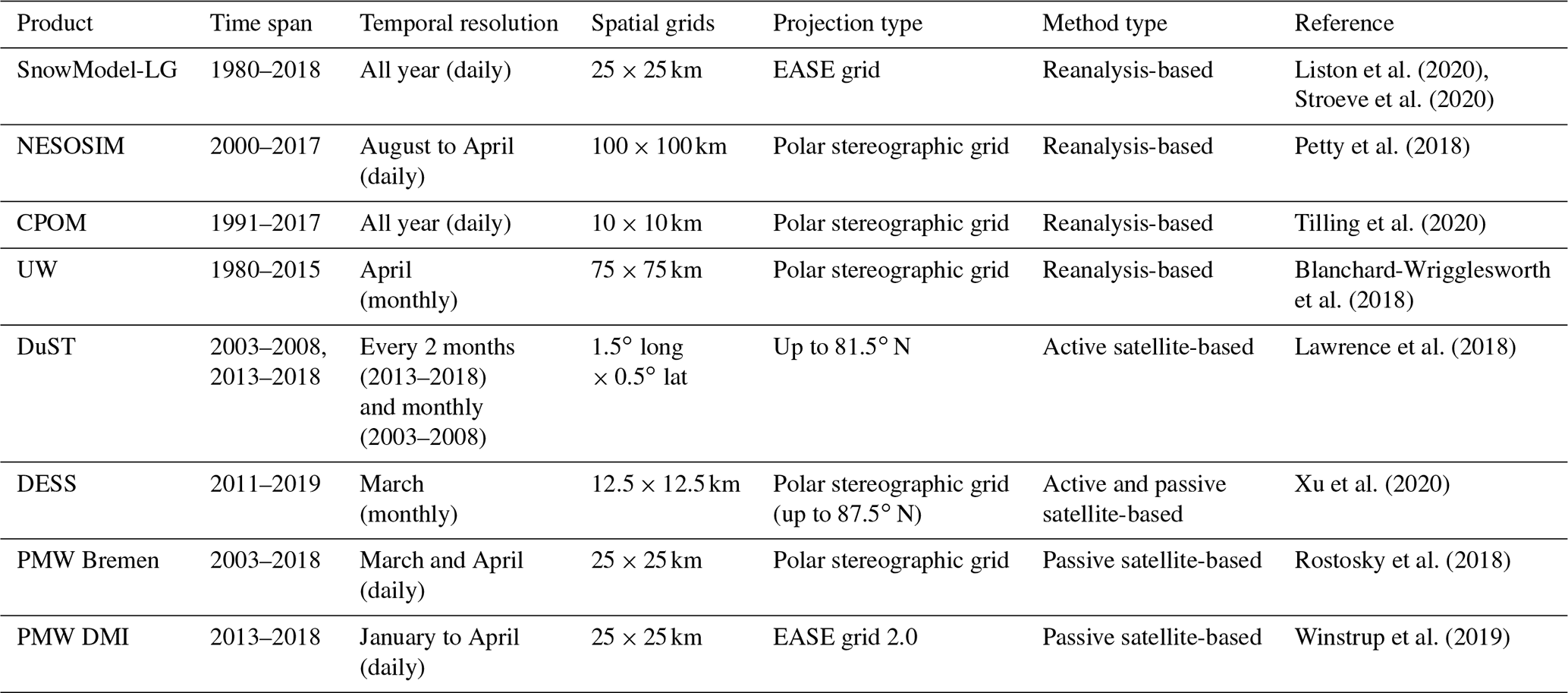

Table 1 Summary of investigated snow reconstruction products.

An additional comparison was made between OIB and the different snow depth products at the coarsest spatial (100×100 km) grid and temporal (monthly) resolution. Below we briefly describe each data set. We refer the reader to the references for each data product for more detailed information on the individual algorithms.

2.1 Measurements used for comparison

2.1.1 In situ observations

Ice mass balance buoys (IMBs) are designed to provide snow depth and ice thickness information and have generally been deployed within undeformed MYI (Richter-Menge et al., 2006). In this study, we use snow depth measurements from IMBs deployed by US Army Cold Regions Research and Engineering Laboratory (CRREL). Each buoy is equipped with acoustic sounders above and below the ice with an accuracy 5 mm for depth measurements (Richter-Menge et al., 2006). Following Perovich et al. (2021), snow depth measurements greater than 2 m or less than 0 m are removed. In total, 58 CRREL buoy tracks are used between 2010 and 2015 (available at: http://imb-crrel-dartmouth.org, last access: 13 January 2021). To align the IMB data with the daily and monthly snow depth products, as well eliminate effects from missing measurements, we average the IMB data into monthly averages after first creating daily averages from the 4-hourly observations. See Table S1 in the Supplement for a listing of buoys used, along with their dates/time periods of operation.

Snow buoys have been deployed by the Alfred Wegener Institute (AWI) since 2010 (Nicolaus et al., 2017) and provide snow depth estimates from four separate snow depth pingers. These are averaged together to provide one snow depth value at each buoy location. Here, we use snow depths from 28 AWI snow buoys between 2013–2017 (accessible at: http://data.meereisportal.de, last access: 13 January 2021), which are also listed in Table S1. Similar to the CREEL buoys, the snow depths are first averaged into daily averages before monthly averages are derived.

2.1.2 OIB airborne observations

Since 2009, NASA Operation IceBridge (OIB) has conducted airborne profiling of Arctic sea ice every spring, generally across the western Arctic. Snow depth observations are derived with an ultra-wideband quicklook snow radar (Paden et al., 2014), capable of retrieving snow depth from the radar echoes from both air–snow and snow–ice interfaces (Kurtz and Farrell, 2011). Snow depth can then be retrieved through retracking and compensation from the radar echogram. The OIB campaigns provide unique large-scale and high-spatial-resolution observations; however, the swath is limited due to the airborne nature of the measurements. Furthermore, most flight tracks cover a limited area from the north of Greenland towards Alaska, and data cover only a limited time period, namely March and April.

Several algorithms have been developed to derive snow depth from this radar system (Kwok et al., 2017). While different algorithms show general agreement in regional snow depth distributions, larger interannual variability is observed among these algorithms than found in W99, and mean snow depth differences result from different ways of detecting the snow–air and snow–ice interfaces from the radar returns (Kwok et al., 2017). Taking these differences into consideration, we use four OIB snow depth products from the (1) Sea Ice Freeboard, Snow Depth, and Thickness data quicklook product (quicklook) available from NSIDC website and examined in King et al. (2015) and Kwok et al. (2017); (2) NASA Goddard Space Flight Center (GSFC) (Kurtz et al., 2013, 2015); (3) Jet Propulsion Laboratory (JPL) (Kwok and Maksym, 2014); and (4) snow radar layer detection (SRLD) (Koenig et al., 2016). These four OIB products overlap only in 2014 and 2015, and thus we limit our comparisons with OIB-derived snow depths to those 2 years. Each OIB product is first regridded to the 100×100 km polar stereographic projection, and then all daily flight tracks are averaged together to produce monthly mean OIB snow depths (March or April) for each year. We also compare snow reconstructions on their native spatiotemporal resolution with OIB measurements in the Supplement.

2.2 Snow depth climatologies

In addition to the airborne and in situ snow measurements, we use two types of conventional large-scale snow products that are often used in the derivation of sea ice thickness from radar or laser altimetry (Ricker et al., 2014; Kwok and Cunningham, 2008), the Warren et al. (1999) (W99) and the Shalina and Sandven (2018) (SS18) climatologies. W99 provides distributions of snow depth and density for each calendar month by assembling North Pole (NP) drifting station observations from the 1950s to 1990s. A two-dimensional quadratic function is adopted to fit the measurements to the Arctic basin. W99 also provides a climatology of snow water equivalent (SWE) from January to December. This is derived using snow depths and densities measured along snow lines, and, if unavailable, Arctic-mean density for that month is used. Like snow depth, a two-dimensional quadratic fit was applied to the SWE data.

SS18 further combines NP data (as in W99) with additional snow data from the Soviet airborne expeditions (Sever) obtained primarily during the 1960s to 1980s to produce spring (March–April–May) snow depth fields. Since the aircraft would land on level FYI, SS18 is not limited to MYI in the central Arctic (as W99) but includes FYI in the Eurasian seas as well (Shalina and Sandven, 2018). The spatial grid spacing of the SS18 climatology is 100×100 km within the Arctic basin.

2.3 Satellite- and model-based snow depth products

Eight snow depth data sets are included in this inter-comparison study (Table 1). They mainly fall into two categories: (1) snow reconstruction using atmospheric reanalysis data as input to a snow accumulation model together with snow redistribution by sea ice drift; (2) snow depth retrieved from satellite data, including passive-microwave-based snow retrieval, blended satellite-derived radar sea ice freeboards at two different frequencies, and active–passive satellite (combining CryoSat-2 and SMOS) data synergy. Here, snow depth is defined as the average thickness of snow over the entire grid-cell area for eight products, not just over the sea-ice-covered fraction.

The first category includes four different new products: the distributed snow evolution model (SnowModel-LG) (Liston et al., 2020; Stroeve et al., 2020), NASA Eulerian Snow on Sea Ice Model (NESOSIM) (Petty et al., 2018), the Centre for Polar Observation and Modelling (CPOM) model (Tilling et al., 2020), and the Lagrangian Ice Tracking System for snowfall over sea ice from the University of Washington (UW) (Blanchard-Wrigglesworth et al., 2018). The second category includes the following snow depth products: the products from the University of Bremen (PMW Bremen) (Rostosky et al., 2018) and the Danish Meteorological Institute (PMW DMI) (Winstrup et al., 2019) rely on satellite passive microwaves at multiple frequencies and polarizations for their snow depth retrieval algorithms. The Dual-altimeter Snow Thickness (DuST) product (Lawrence et al., 2018) is derived from combining data from CryoSat-2 (Ku band) and AltiKa (Ka band) satellite radar altimeters. The DuST product also combines Envisat (radar altimeter: Ku band) and ICESat (laser altimeter) data during their period of overlap. Finally, Department of Earth System Science in Tsinghua University (DESS) combines a Ku-band altimeter (CryoSat-2) and L-band passive microwave radiometer (SMOS) to retrieve snow depth and sea ice thickness based on two physical models (Xu et al., 2020). Each approach uses vastly different methodologies and provides snow information at different spatial and temporal resolutions.

2.3.1 Reanalysis-based snow depth reconstruction

SnowModel-LG

SnowModel-LG is a prognostic snow model originally developed for terrestrial snow applications, now adapted for snow depth reconstruction over sea ice using Lagrangian ice parcel tracking (Liston et al., 2020). Physical snow processes are included such as blowing snow redistribution and sublimation, density evolution, and snowpack metamorphosis. SnowModel-LG is used in a Lagrangian framework to redistribute snow around the Arctic basin as the sea ice moves. Tracking begins on 1 August 1980, assuming snow-free initial conditions, and accumulates snow until 31 July of the next year. On 31 July, any remaining snow that is isothermal and saturated with meltwater becomes superimposed ice and is no longer identified as “snow”. SnowModel-LG is the only data product that includes snow depth during the melt season. The essential inputs to this data product are atmospheric reanalysis estimates of precipitation, 2 m air temperature, wind speed and direction, and weekly ice motion vectors from NSIDC (Stroeve et al., 2020). Weekly ice motion vectors are linearly interpolated to daily resolution. Outputs relevant to this study are the snow depth and bulk snow density (Liston et al., 2020) and are provided on a 25×25 km EASE grid. A recent study (Stroeve et al., 2020) evaluated SnowModel-LG using NASA MERRA-2 (Gelaro et al., 2017) and ERA5 atmospheric reanalysis fields (Hersbach and Dee, 2016) against several data sets including OIB, IMBs, MagnaProbe and passive microwave estimates. They found that the model captured observed spatial and seasonal variability in snow depth accumulation, while also showing statistically significant declines in snow depth since 1980 during the cold season. The temporal resolution of SnowModel-LG is daily between 1 August 1980 and 31 July 2018.

NESOSIM

The NASA Eulerian Snow On Sea Ice Model (NESOSIM) is a three-dimensional, two-layer (vertical), Eulerian snow budget model (Petty et al., 2018). NESOSIM includes two snow layers: old compacted snow and new fresh snow. Wind-packing and snow loss to the leads are included and were used to calibrate NESOSIM with historical snow depth and density observations from the NP drifting station data. NESOSIM was run using several atmospheric reanalyses, including ERA-Interim (ERA-I) (Dee et al., 2011), JRA-55 (Ebita et al., 2011) and MERRA (Rienecker et al., 2011), and a median of these daily reanalysis snowfall estimates is used in this study. The model is also forced with near-surface wind fields from ERA-I, NSIDC Polar Pathfinder sea ice drift vectors (Tschudi et al., 2019) and Bootstrap passive microwave ice concentrations (Comiso, 2017). Snow accumulation is initialized at the end of summer (default of 15 August) and run until the following spring (1 May). To initialize snow depth in mid-August, NESOSIM linearly scales the August snow depth in the W99 climatology based on the ratio between duration of the summer melt season and the climatological summer duration. The duration of the summer melt season is defined based on ERA-I air temperatures, and climatological summer melt duration is from Radionov et al. (1997). Snow depth is further equally divided into the “old” and “new” snow layers, with snow transferred from the new to the old snow layer based on the wind conditions. Snow is then accumulated and evolves dynamically with sea ice motion through a divergence–convergence and an advection term. Daily snow depth (mean depth over the sea ice fraction) and snow density and snow volume (per unit grid cell) are available from 15 August to 30 April for each year, at a spatial grid spacing of 100×100 km in a polar stereographic projection. NESOSIM provides the effective snow depth of the ice-covered fraction and the mean grid-cell snow depth. In order to be consistent with snow depth estimates from the other methods, we will use the latter in this study.

CPOM

The CPOM snow depth product (Tilling et al., 2020) is initialized on a Lagrangian grid with a spacing of 10 km running from 40^∘ N to the pole. Snow accumulation begins on 15 August each year using the W99 August snow depth and a fixed density of 350 kg m⁻³ on all ice-covered (sea ice concentration >15 %) grid points. This initial snow layer is kept separated from any accumulated snow after the model has started running. The model then steps daily through the winter, accumulating snow in SWE. Snow parcels are moved using NSIDC Polar Pathfinder ice motion data, and any parcels moving outside the ice-covered region are removed. New parcels covered by expansion of the ice-covered region become active with no initial snow. Where the 2 m ERA-I air temperature is above freezing point, the daily ERA-I SWE of snowfall is added to the already accumulated column. A fraction of the accumulated snow is removed when the wind speed exceeds 5 m s⁻¹ using a function proportional to wind speed and lead fraction (see Schröder et al., 2019, Table 1). Finally, the total column of accumulated SWE at each Lagrangian point is converted to snow depth using a daily snow density function constructed in a similar way to Kwok and Cunningham (2008), which is added to the initial snow layer (if present). The irregularly spaced snow data from the Lagrangian grid are re-gridded onto a regular 10 km² polar stereographic projection using an averaging radius of 50 km to give a snow depth map for each day of winter.

UW

The last reanalysis-based snow reconstruction is from the University of Washington (UW). The algorithm accumulates cold-season snowfall along sea ice drift trajectories using 12-hourly snowfall from ERA-I, weekly NSIDC sea ice vectors and weekly-averaged NOAA-NSIDC sea ice concentration (Meier et al., 2013). A Lagrangian Ice Tracking System (LITS) (DeRepentigny et al., 2016) is used to backward track each grid point from the first week of April to the last week of the previous August (Blanchard-Wrigglesworth et al., 2018). This tracking system has a claimed accuracy of ≈50 km after 6 months of tracking (DeRepentigny et al., 2016). Once the 6-month trajectories are established for each ice parcel, the algorithm accumulates weekly-averaged snowfall along each parcel trajectory. A sea ice concentration correction is further imposed every week (one time step). Specifically, if the ice concentration drops below 15 %, the accumulation stops and the trajectory is ended at the previous time step. Only monthly snow depths in April are available for the period from 1980 to 2015. Spatial grid spacing of the data set is 75×75 km on a polar stereographic projection.

2.3.2 Satellite-based snow depth retrieval

DuST

Lawrence et al. (2018) derives snow depth by utilizing the difference in freeboards retrieved from radar altimeter satellites operating at different frequencies. Specifically, satellite data from ESA's CryoSat-2 (CS-2, Ku-band radar satellite altimeter operational since 2010) and CNES/ISRO's AltiKa (Ka-band radar satellite altimeter, 2013–present) are used. The deviation of each satellite's return from its expected dominant scattering horizon (the snow surface for the Ka band and the ice–snow interface for the Ku band) is quantified using independent snow and ice freeboards from OIB. Using a spatially variable correction function, AltiKa and CS-2 freeboards are calibrated to the snow surface and snow–ice interfaces, respectively, allowing snow depth to be estimated as the difference between the two. A caveat to the approach is that since OIB data are only available during March and April and cover limited regions of the Arctic, the calibration of the CS-2 and AltiKa freeboards with OIB may not be valid during other months and/or regions. The same methodology has also been applied to ICESat and Envisat satellites, whose active periods overlap between 2003 and 2009, and these data are used to extend the snow depth product further back in time. This Dual-altimeter Snow Thickness (DuST) product produces (1) monthly snow depth maps from October to April during the CS-2/AltiKa period (2013–present) and (2) bimonthly (every 2 months) annual snow depth maps (March–April or October–November) during the ICESat–Envisat period (2003–2008). For both time periods, the snow depth is gridded on a 1.5^∘ longitude × 0.5^∘ latitude grid. The data are limited to below 81.5^∘ N due to the upper latitude of AltiKa/Envisat.

PMW Bremen

The University of Bremen's PMW snow depth product described in Rostosky et al. (2018) on FYI is available during the AMSR-E/2 period. The algorithm is adapted from Markus and Cavalieri (1998), which was derived from a series of passive microwave sensors, such as the Scanning Multichannel Microwave Radiometer (SMMR) (from 1979), and continuing on through the Special Sensor Microwave/Imager (SSM/I) and SSM/I Sounder (SSMIS). The latter algorithm computes the spectral gradient ratio between 18.7 and 37 GHz vertical polarization brightness temperatures (Tbs) to generate 5 d averaged snow depth estimations over FYI (Markus et al., 2011). This algorithm has limitations for wet snow spring and multiyear ice (Comiso et al., 2003) and large sensitivity to surface roughness (Stroeve et al., 2006). Snow depths over smooth FYI were found to be accurate in comparisons with OIB during 2009 and 2011 (RMSE <0.06 m over a shallow snow cover), while significant biases were found over rougher FYI or MYI (Brucker and Markus, 2013).

Rostosky et al. (2018) further extends the approach of Markus and Cavalieri (1998) to also include snow depth over MYI using the lower frequencies of 6.9 GHz from the NASA Advanced Microwave Scanning Radiometer for the Earth Observing System (AMSR-E) and the JAXA Global Change Observation Mission – Water (GCOM-W) AMSR2 instrument. We refer to the resulting product as the PMW Bremen snow depth product. The gradient ratio between vertical polarized brightness temperatures (Tbs) at 18.7 GHz and 6.9 GHz helps to mitigate the retrieval sensitivity problems over MYI during March and April. Specifically, robust linear regressions were derived based on fitting 5 year (2009, 2010, 2011, 2014, and 2015) of the NOAA Wavelet (WAV) Airborne Snow Radar-Snow Depth on Arctic Sea Ice Data Set (Newman et al., 2014) and the polarized Tb gradient ratio. Snow depths over different ice types were fitted separately, using the Ocean and Sea Ice Satellite Application Facility (OSI-SAF) sea ice type map to distinguish between FYI and MYI. No evaluation/validation was performed in regions outside of OIB measurements. The spatial grid spacing is similar to typical passive microwave measurements, at 25×25 km in the polar stereographic projection. Daily snow depth maps for winter months from November to April since 2002 are available. It should be noted that snow depth over MYI is only available during March and April when the OIB data were available to constrain the model. Snow depth uncertainty is estimated to be between 0.1 and 6.0 cm over FYI and between 3.4 and 9.4 cm over MYI.

PMW DMI

In Winstrup et al. (2019), snow depth is derived by a random forest regression model based on passive microwave Tbs from AMSR-E and AMSR2. The model was trained using a Round-Robin Data Package (Pedersen et al., 2018), with OIB campaigns snow thicknesses provided by NSIDC including IDCSI4 and quicklook products and collocated brightness temperatures. Training was performed on two-thirds of the data set, using OIB data from the period April 2009–March 2014, leaving the remaining OIB data (period: March 2014–April 2015) for validation purposes. Specifically, multi-channel Tbs ranging from the C band (6.9 GHz) to 89 GHz are included as predictors, at both vertical and horizontal polarization. The random forest consists of 500 regression trees, each derived from bootstrapping the input data and using a maximum limit of five predictors for each leaf in the regression trees. The most important predictors, as found by the algorithm, were the following channels: 18.7 GHz (27 %), 23.8 GHz (17 %) and 10.7 GHz (11 %), all vertical polarizations. Derived snow depths were found to be in good agreement with the OIB data retained for validation, with an average error of 0.05 m and an accuracy of 78.7 %. The passive microwave snow depth product from the Danish Meteorological Institute (PMW DMI) constructs springtime (March and April) daily snow depth between 2013 and 2018 at 25×25 km spatial grid spacing on the EASE-Grid 2.0 (Brodzik et al., 2012).

DESS

The Department of Earth System Science in Tsinghua University (DESS) algorithm retrieves both sea ice thickness and snow depth simultaneously by using sea ice freeboard from CS2 and the L band (1.4 GHz) Tbs from the Soil Moisture and Ocean Salinity (SMOS) satellite (Xu et al., 2020). The active periods of these two satellites are both from 2010 to present. Specifically, this algorithm combines a hydrostatic equilibrium model and improved L-band radiation model (Xu et al., 2017). Sea ice freeboard is converted to sea ice thickness based on hydrostatic equilibrium (Laxon et al., 2003), using assumptions on snow, ice and water densities. Tbs from SMOS can be used to retrieve thin sea ice thickness (Kaleschke et al., 2012) and snow depth over thick ice (Maaß et al., 2013). The L-band radiation model is further improved by adding vertical structure of temperature and salinity in sea ice and snow (Zhou et al., 2017). In order to obtain the missing measurements resulting from limited upper latitude in the SMOS satellite, L-band Tbs spanning inclination angles from 0 to 40^∘ and from 85 to 87.5^∘ N are approximated using Tbs of all frequencies in AMSR-E and AMSR2 through a back-propagation machine-learning process. By combining the two observational data sets, the uncertainties in both sea ice thickness and snow depth are largely reduced. Unlike optimal interpolation-based sea ice thickness synergy, as applied in Ricker et al. (2017), the uncertainty in ice thickness is reduced through an explicitly retrieved snow depth.

Both sea ice thickness and snow depth are available in the DESS product. Here we use the monthly snow depth maps available for March of each year since 2011, which are provided at a spatial grid spacing of 12.5×12.5 km on a polar stereographic projection.

3 Snow products inter-comparison

In this section, we carry out a systematic comparison of the eight snow products, using the two climatological snow data sets (W99 and SS18) as a reference for all comparisons and analyses. Section 3.1 presents the results for mean snow depth and its spatial distribution, Sect. 3.2 introduces the seasonal cycle, and the long-term trend and interannual variability is presented in Sect. 3.3. For the two products that model an evolving snow density, we also intercompare these against climatology (Sect. 3.4). While we focus on basin-wide estimates for the whole Arctic, we also explore consistency and mean state of all products over three sub-regions: the Canadian Arctic sector (CA) including the Canadian Arctic Archipelago, the Atlantic (Atlantic), and the Pacific and Central Arctic (Pacific) sectors (regions outlined in Fig. S1). Over these regions, sea ice conditions vary considerably, with mostly thick MYI within the CA and thinner FYI elsewhere. The North Atlantic has generally more precipitation as a result of proximity to the North Atlantic storm tracks.

Given the relatively long time period and basin-scale coverage provided by SnowModel-LG, this snow depth product is used as the reference product when carrying out the regional consistency checks. To align the temporal and spatial resolution between all snow products, comparisons are mainly carried out after year 2000 and focused on the early and late winter months of October and/or November and March and/or April. The products containing data for longer time periods are further explored against climatologies, and their long-term trends are assessed.

3.1 Mean state and distribution of snow depth

Mean snow depth, which is a direct indicator of total snow volume over sea ice, is of fundamental importance for the characterization of the Arctic hydrological cycle. Spatial maps of monthly mean snow depth across all data products, as well as the W99 and SS18 climatologies, are shown in Figs. 2 and 3 in spring (autumn) months for the season of 2014–2015. Products are shown with their native resolution and grids. The spatial patterns in all products are in broad agreement that thicker snow occurs north of Greenland and the CA sector and thinner snow in the seasonal ice zones (i.e., Baffin Bay and marginal seas of the Eurasia continent). Some products also show thicker snow in the East Greenland Sea (NESOSIM in particular) and the Atlantic sector of the Arctic. Despite some general agreements, mean spring snowpack and regional discrepancies are evident in Fig. 2. In particular, the thickest snow in late winter/early spring for NESOSIM occurs in the East Greenland Sea, while in DESS the deepest snow is concentrated in the Canadian Arctic.

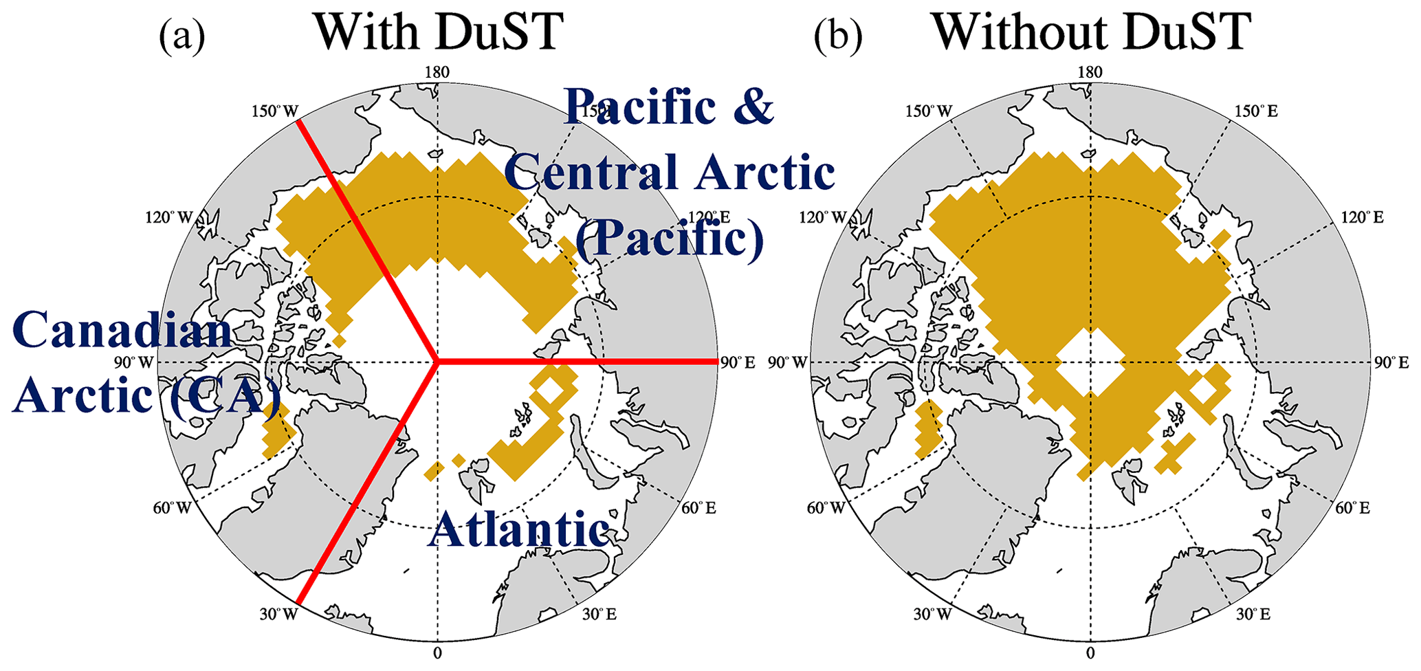
Figure 1 The common regions (yellow) of snow product inter-comparison with (a) and without (b) DuST. Also shown are the regions of interest in this study: Canadian Arctic (CA), North Atlantic sector (Atlantic), and Pacific and Central Arctic (Pacific).

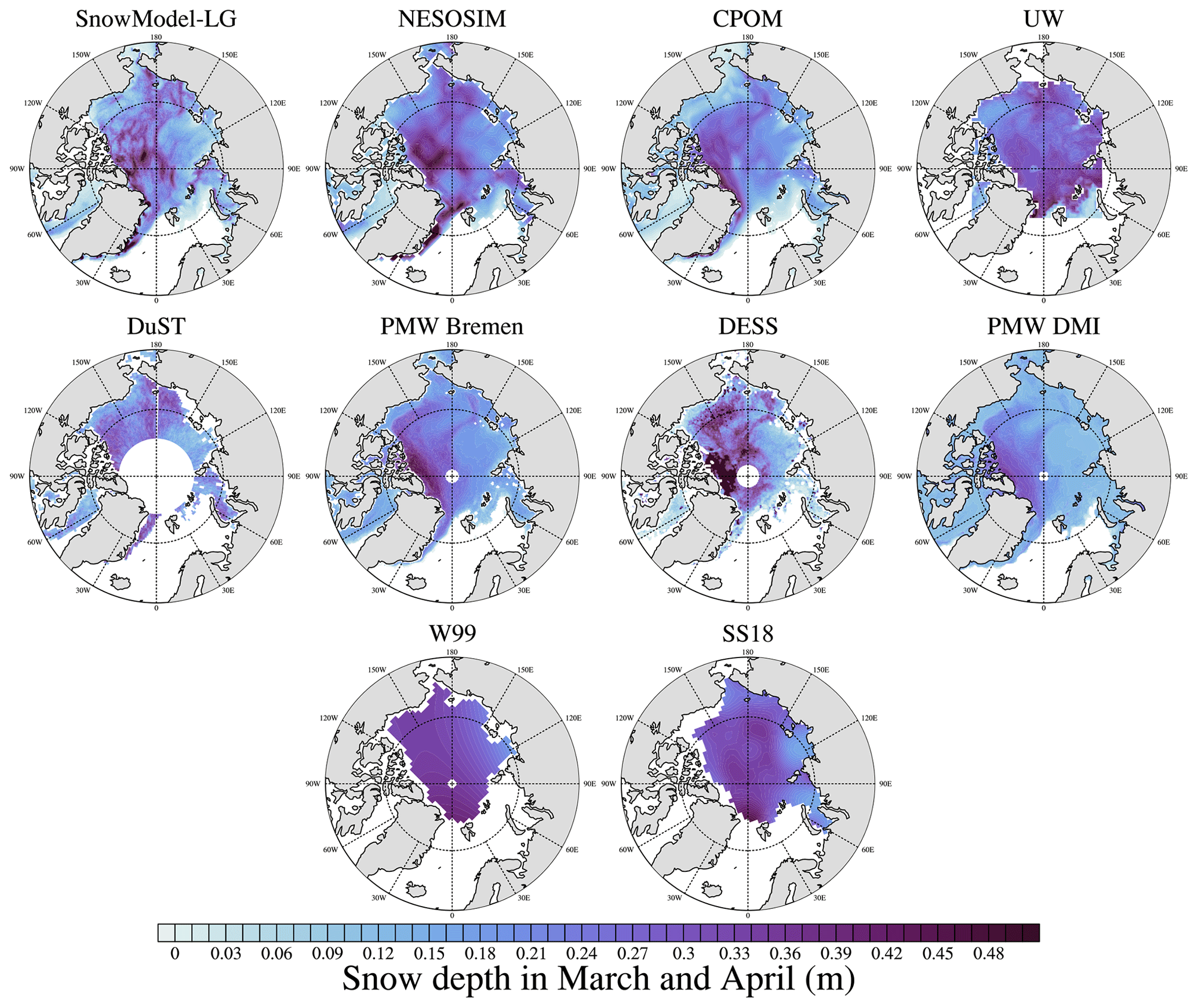
Figure 2 Mean snow depth (units: m) in spring (March–April) 2014 for eight snow products, W99 and SS18.

Figure 3 Mean snow depth (units: m) in autumn (October–November) 2014 for four snow products and W99.

During autumn, for the region north of Greenland and Svalbard, SnowModel-LG runs forced with MERRA-2 show a similar spatial pattern to other reanalysis-based modeling systems (i.e., NESOSIM and CPOM) but shallower snow than NESOSIM (Fig. 3). DuST also shows deep snowpacks in this region (16.6 cm mean snow depth), though the spatial coverage is more limited. Spring snow depth, ranging from 15.2 to 25.3 cm in the Arctic domain (Fig. 1), exhibits large spatial variability among all products. Further, relatively thick snowpacks in the North Atlantic sector are evident in all reanalysis-based products except for CPOM. Deeper snowpacks are expected in this region as it receives winter precipitation from the North Atlantic storm tracks. The discrepancies in spring among the reanalysis-based products are the results of several aspects including initial snow assumption, tracking numerical algorithm and reanalysis adoption. For comparison, snow is also the deepest (over 35 cm) to the north of Svalbard in both the W99 and SS18 climatologies. NESOSIM further suggests thick snow over Davis Strait, with spring averaged snow depths greater than 25 cm. This is in stark contrast to the other data sets over the FYI in that region and is likely unrealistic given this is a region of first-year ice that does not usually freeze until December and/or January, e.g., Stroeve et al. (2014), limiting the time over which snow can accumulate on the ice.

The histogram of time-averaged snow depth in the different products is shown in Fig. 4 for the period 2000 to 2018 during the spring and autumn periods, respectively. Out of all the reanalysis-based data products, snow depth distributions in NESOSIM are shifted towards slightly deeper snowpacks (8.4 cm) than those from SnowModel-LG (7.2 cm) and CPOM (6.0 cm) during autumn, although the shapes of the distributions are similar. The deepest snowpacks during October and/or November are found in DuST, with a mode of the distribution at about 16.6 cm. This is much larger than other products and seems unlikely to be realistic early in the snow accumulation season. During spring (Fig. 4b), PMW DMI exhibits the overall smallest snow depth in late winter (14.5 cm), while UW shows the largest snow depth (25.2 cm) in the common region of the snow products. Conclusions are similar if we omit DuST and extend the analysis up to 87.5^∘ N. Doing so, the bimodal snow depth distribution in autumn is more evident, suggesting more snow cover over old sea ice north of 81.5^∘ N. As expected, snow depths shift to overall deeper snowpacks in spring, especially when including the higher latitudes (Fig. 4c and d). The shallowest spring snow in PMW DMI, with a mean snow depth <15 cm, and the thickest autumn snow in DuST are the two extremes among current snow products.

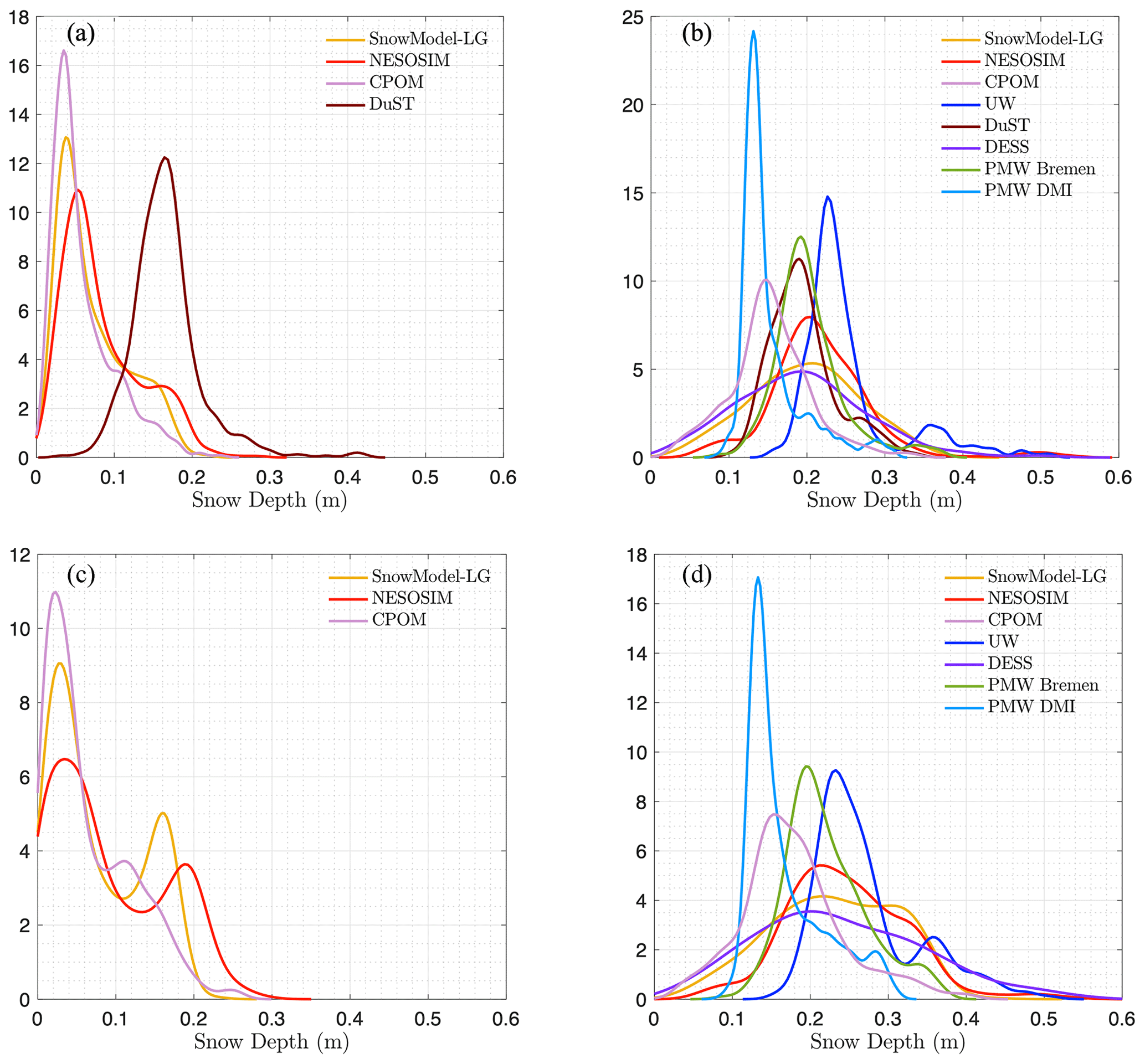
Figure 4 Snow distribution comparison within the common regions (in Fig. 1a) in all snow products during the period 2000–2018 (different products cover different periods) with/without DuST included in October–November (a, c) and March–April (b, d).

Additionally, we examine snow depth over the three different sectors in spring 2015 (Fig. S1 in the Supplement). The deepest snowpacks from reanalysis-based snow products mainly occur over the North Atlantic, while satellite-based products indicate more snow accumulating over the CA. Although this is only 1 year of comparison, it shows that regional differences in snow accumulation can be quite pronounced depending on the data set used.

Discrepancies between snow products and the climatologies both in spring (Fig. 5) and in autumn (Fig. S2) are evident. In autumn (Fig. S2), bimodal snow distributions are noticeable both in SnowModel-LG and NESOSIM using the data past 2000, with a large proportion of thin snow not seen in the W99 climatology. By the end of winter, the differences between all products and W99 are larger (Fig. 5) than in autumn, with the minimum decreasing being 10 cm for UW and the maximum being over 15 cm for PMW DMI in spring. SnowModel-LG, DuST and DESS all have snow depths below 10 cm in March and/or April. For reanalysis-based products, the snowpack is still significantly shallower against climatologies in the 1980s (1990s in the case of CPOM) when W99 is partly collected. In addition to mean snow depth, the skewness of the snow distribution, especially in spring, among all products is mainly positive as a result of the larger presence of thin snow cover over FYI dominated in the current era, while that of W99 is the opposite.

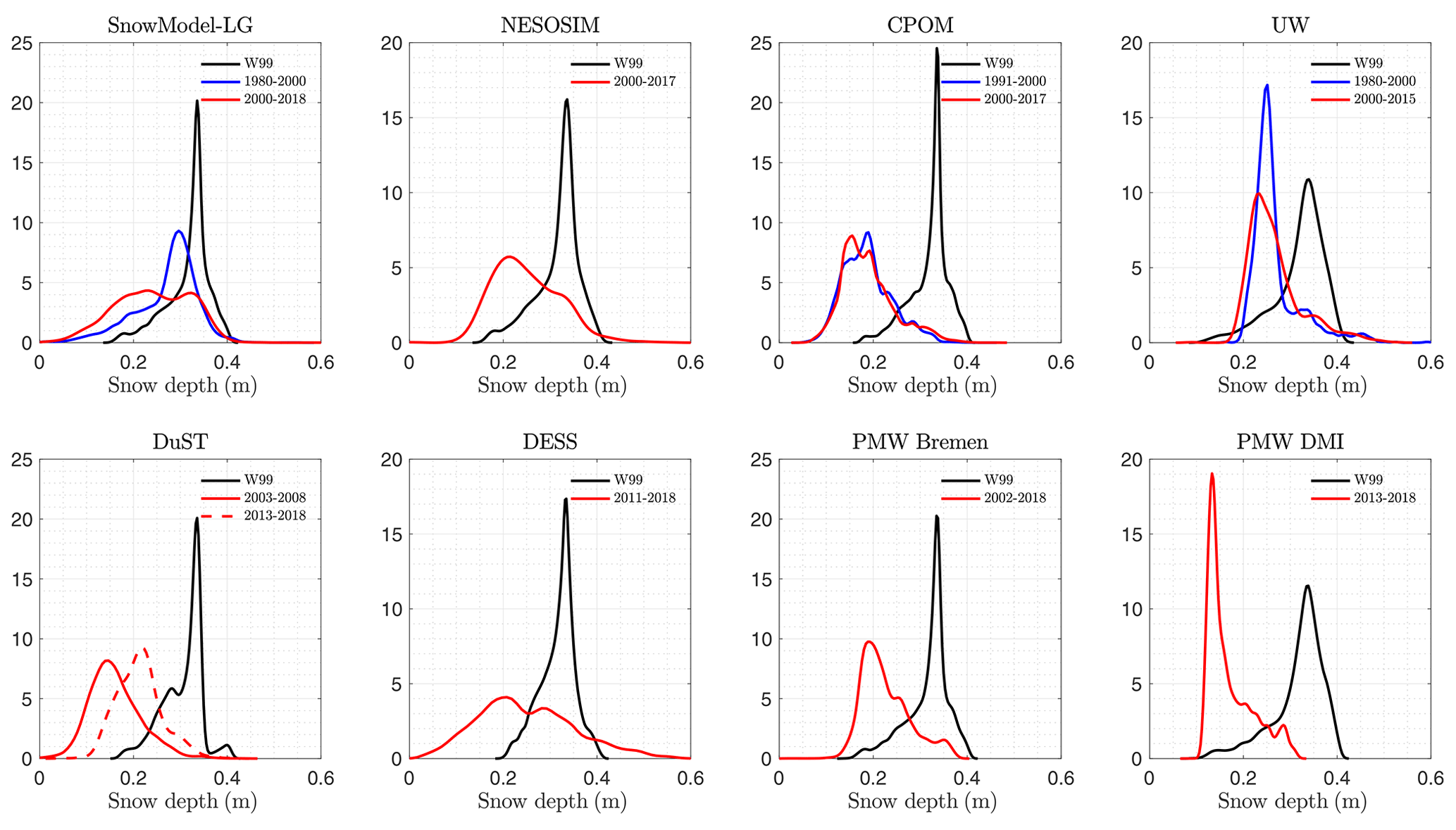
Figure 5 Snow distribution comparison between W99 and snow products in spring (March and/or April).

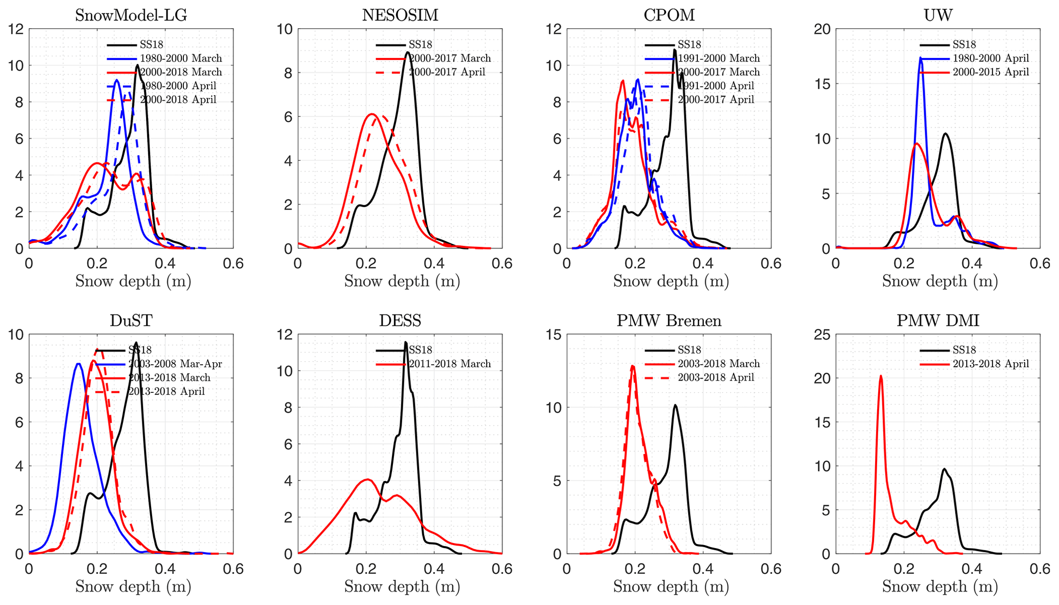
Apart from W99, the Shalina and Sandven (2018) climatology provides additional snow depth information in the marginal seas, especially over the Eurasian seas. Overall SS18 has lower snow depths in the central Arctic compared with W99. Figure 6 reveals that snow distribution in SS18 includes two modes – 18.1 and 32.2 cm – which correspond to snow over FYI and MYI respectively. Generally, differences between the SS18 climatology and the various snow products are similar to the comparison results with W99, but SS18 tends to exhibit a similar bimodal distribution to that seen in some of the snow products.

Figure 6 Snow distribution comparison between SS18 climatology and snow products.

To summarize, there is general agreement among the products (except for UW) that there is a distinct difference in snow depth on perennial and seasonal ice. It is worth noting that this agreement is across the two distinctive methods for snow depth reconstruction, i.e., the reanalysis-based numerical integration and satellite-based retrievals. This is also reflected in both the basin-scale snow depth averages and the spatial patterns. However, the areas where the thickest/thinnest snow depths are found tend to differ between the two types of methods. The heavy snow in reanalysis-based products falls primarily over the East Greenland Sea and Atlantic sector as a result of frequent storm tracks over this area, whereas from active or passive microwave satellite data the thickest snow is detected over the Canadian Arctic sector due to the different features of old vs. newly formed ice. Finally, the intercomparison of the different snow products, and further against two climatological data sets, reaches similar conclusions: (1) all snow products have similar structure such that snow over perennial ice is thicker, but with quite large regional differences in mean value; and (2) snow depths in the products evaluated show less snow in recent years relative to the climatologies.

3.2 Seasonal cycle of snow depth

Time series (2000–2018) of monthly mean snow depths during winter (September to April) averaged over regions up to 81.5^∘ N are displayed in Fig. 7, whereas Fig. 8 shows the seasonal mean and spread. The W99 is included as reference (see Fig. S3 for the results when the region is extended up to 87.5^∘ N).

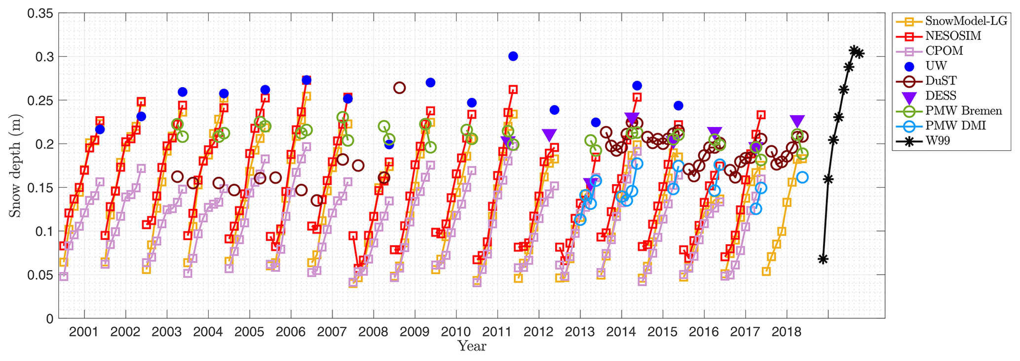
Figure 7 Time series of average monthly snow depth in each snow product within the common regions since 2000. Only wintertime (September to next April) is shown.

Figure 8 Wintertime snow accumulation among eight products and W99 since 2000.

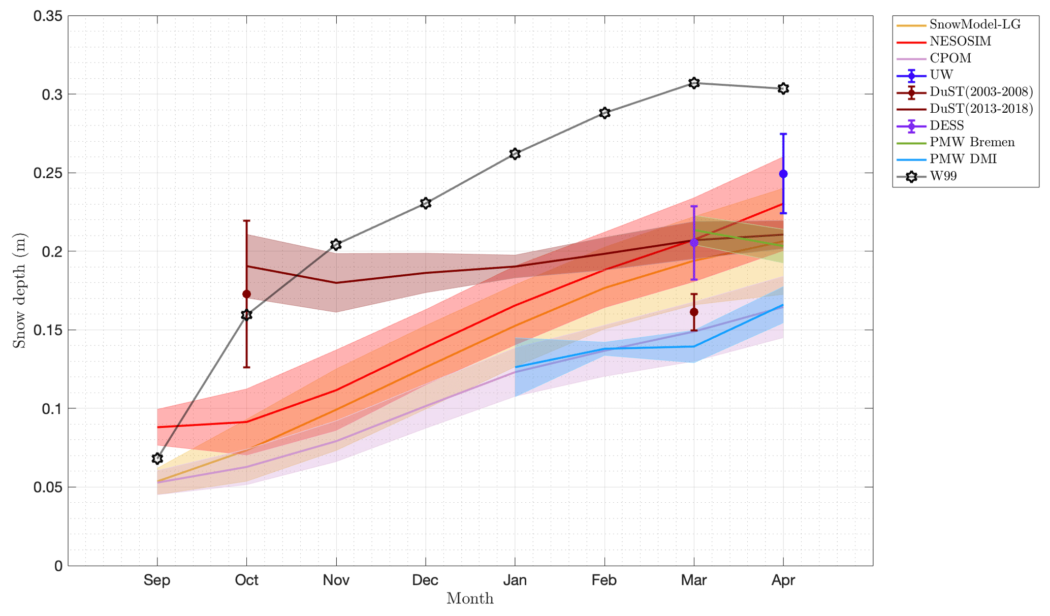
In NESOSIM, April snow depths are higher than in SnowModel-LG (Fig. 7), especially after 2012. We further see from Fig. 8 that the initial snow depth before autumn is thinner in SnowModel-LG, but there is more wintertime snow accumulation in SnowModel-LG than in NESOSIM. Thicker autumn snow in NESOSIM is a result of using W99 for the initial conditions, while SnowModel-LG tracks the snow through the summer melt season, removing any remaining snow at the end of summer when the snowpack is saturated and isothermal (this then becomes decomposed ice). The end result is that by the end of winter overall differences between the two products are less pronounced despite large differences in total snow accumulated over winter.

Seasonal snow accumulation is also larger in SnowModel-LG compared with CPOM. In contrast, the seasonal accumulation in DuST and snow changes from March to April in PMW Bremen are unexpectedly small, even negative, while the PMW DMI shows similar seasonal changes to the reanalysis-based products. Overall, the largest seasonal snow accumulation occurs in W99, and the deepest snowpacks are observed in March, the month when snow reaches its maximum depth, whereas many of the other products reach their maximum snow depths in April. However, based on Sect. 3.1, compared with W99, all snow cover products in early winter have thinner snowpacks than at the end of the winter, which implies either that the intensity of snow accumulation is weakening or that the snow accumulation period has shortened. We further note that W99 accumulates more snow during the early part of winter, and thus the seasonal curves are flattened near spring. SnowModel-LG, NESOSIM and CPOM on the other hand share similar seasonal accumulation curves, with accumulation continuing to increase through winter. This seasonal pattern of winter snow accumulation finds support in a recent study by Kwok et al. (2020) that found accumulation later in winter in 2018–2019. This implies that there may be limited efficacy of the climatological seasonal pattern of snow accumulation in the current Arctic climate. As sea ice freeze-up continues to delay further over the last 40 years, it is expected that the early snow accumulation will continue to differ from that reflected in W99.

3.3 Trend and interannual variability of snow depth

All reanalysis-based snow reconstructions, namely SnowModel-LG, CPOM, NESOSIM and UW, have consistent interannual variability in spring snow volume from 2000 to present (see details in Table S2), with statistically significant (confidence level 99 %) correlations of the interannual snow depth/volume between the data sets. DESS also exhibits generally similar interannual variability to the reanalysis-based products (R²=0.42 for SnowModel-LG, 0.68 for NESOSIM and 0.32 for CPOM), whereas PMW Bremen and DuST do not.

While there is interannual variability in snow accumulation, the variability is overall quite small, ranging from 2 cm in November to about 2 to 3 cm in April. This also holds for results as averaged up to 87.5^∘ N (Fig. S3). The interannual variability seen in the data products is about half of that previously reported in W99, where interannual variability was estimated to be about 4.3 cm in November and 6.1 cm in April. It is important to note, however, the climatological estimation of interannual variability in W99 includes snow depth uncertainties and should be treated as an upper bound for the inherent physical interannual variability. It should be also noticed that DuST shows a significant positive snow depth bias from the Envisat period to the CryoSat-2 period, likely a result of using OIB to calibrate the snow depth estimates. This positive snow bias is missing in the passive-microwave-based snow products (e.g., PMW Bremen) and is not observed in DESS (time series in PMW DMI is too short to be assessed).

As averaged over the common regions of all data sets, no significant trend is observed in most snow products except DuST since 2000. However, regionally the reanalysis-based snow products exhibit regions of statistically significant positive and negative snow depth trends over a longer time period. For example, positive snow depth trends are found north of Greenland and the Canadian Arctic Archipelago from 1991 to 2015 (common period) (Fig. 9). These positive trends may be a result of more autumn precipitation (Serreze et al., 2012) or changes in the proportion of MYI vs. FYI in the region. On the other hand, snow depth trends in spring are mostly negative within the rest of the Arctic basin and statistically significant for SnowModel-LG in FYI regions and for CPOM in the Barents Sea. In autumn, the regions with statistically significant negative snow depth trends in SnowModel-LG are larger, which is likely a result of delays in freeze-up (Markus et al., 2009; Stroeve and Notz, 2018). CPOM also shows negative trends in these regions but not as large as those from SnowModel-LG. April and November mean snow depth trends from SnowModel-LG as computed over the entire Arctic basin are −0.5 and −0.9 cm per decade, respectively, although some regions show larger trends. In CPOM, a basin-mean significantly negative trend (−0.47 cm decade⁻¹) is only found in November.

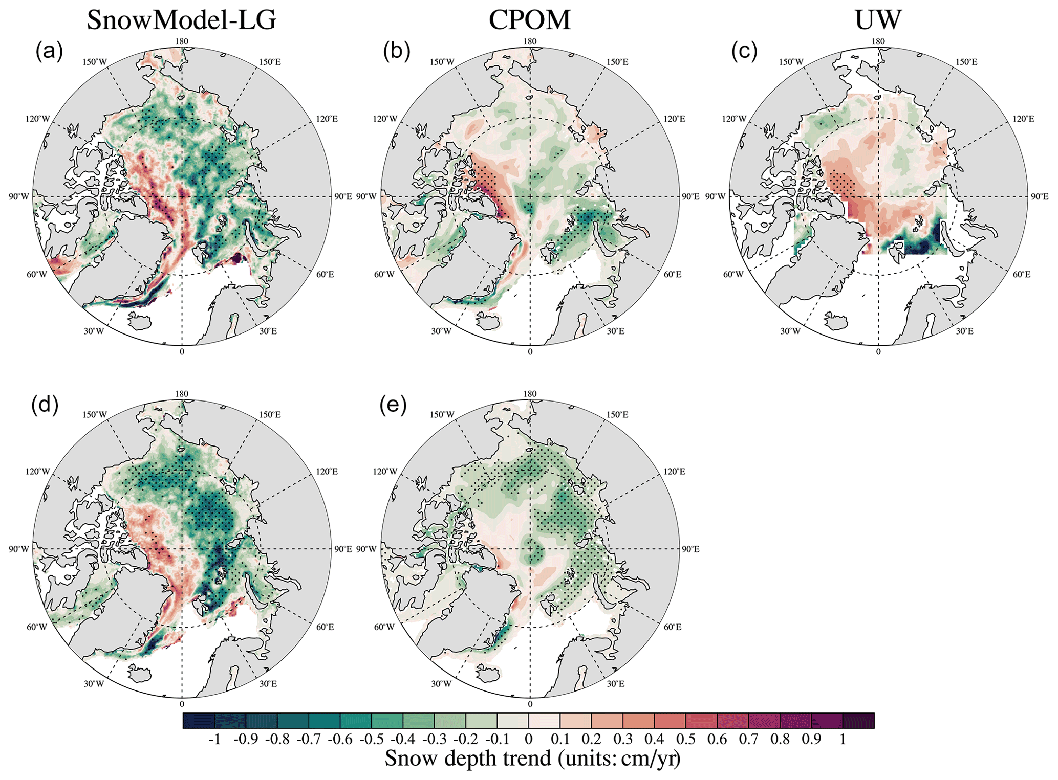
Figure 9 Trend of snow depth (units: cm yr⁻¹) for SnowModel-LG, CPOM and UW in spring (April) (a–c) and autumn (November) (d, e) during the period from 1991 to 2015. Areas with significant trends are shown as dotted areas (confidence level 95 %).

Finally, we synthesize long-term changes in snow depth in relationship to the climatology products. As mentioned in Sect. 3.1, the minimum and maximum differences of mean snow depth in March and/or April between products in the current years and climatology are 10 and 15 cm respectively over the last 40 years; thus the inter-decadal snow depth changes would be in the range of −0.25 and −0.375 cm yr⁻¹. These estimates span the value of −0.29 cm yr⁻¹ in Webster et al. (2014). However, one should keep in mind that there are large uncertainties in the snow climatology data sets, and the interannual variability is larger than in the snow products.

3.4 Snow density comparison

Apart from snow depth, we further investigate snow density in the two products that provide snow density estimates: SnowModel-LG and NESOSIM. Since the W99 climatology contains both snow depth and SWE, we can compare against the W99 snow densities. Snow density in W99 is limited to the Arctic basin. SnowModel-LG suggests that snow is denser than in NESOSIM in both November and April, as shown in Fig. 10. Considering that the snow depth in SnowModel-LG is thinner than NESOSIM, we find that the two models provide a broadly equivalent SWE (not shown). Snow over the Atlantic sector, especially within the East Greenland Sea, is the densest in SnowModel-LG, with mean density values above 370 kg m⁻³ in November and April. In contrast, NESOSIM has mostly smaller snow densities and considerably less spatial variability. For W99, the snow is denser over the Atlantic sector in November, while in April the denser snow is over the Pacific sector.

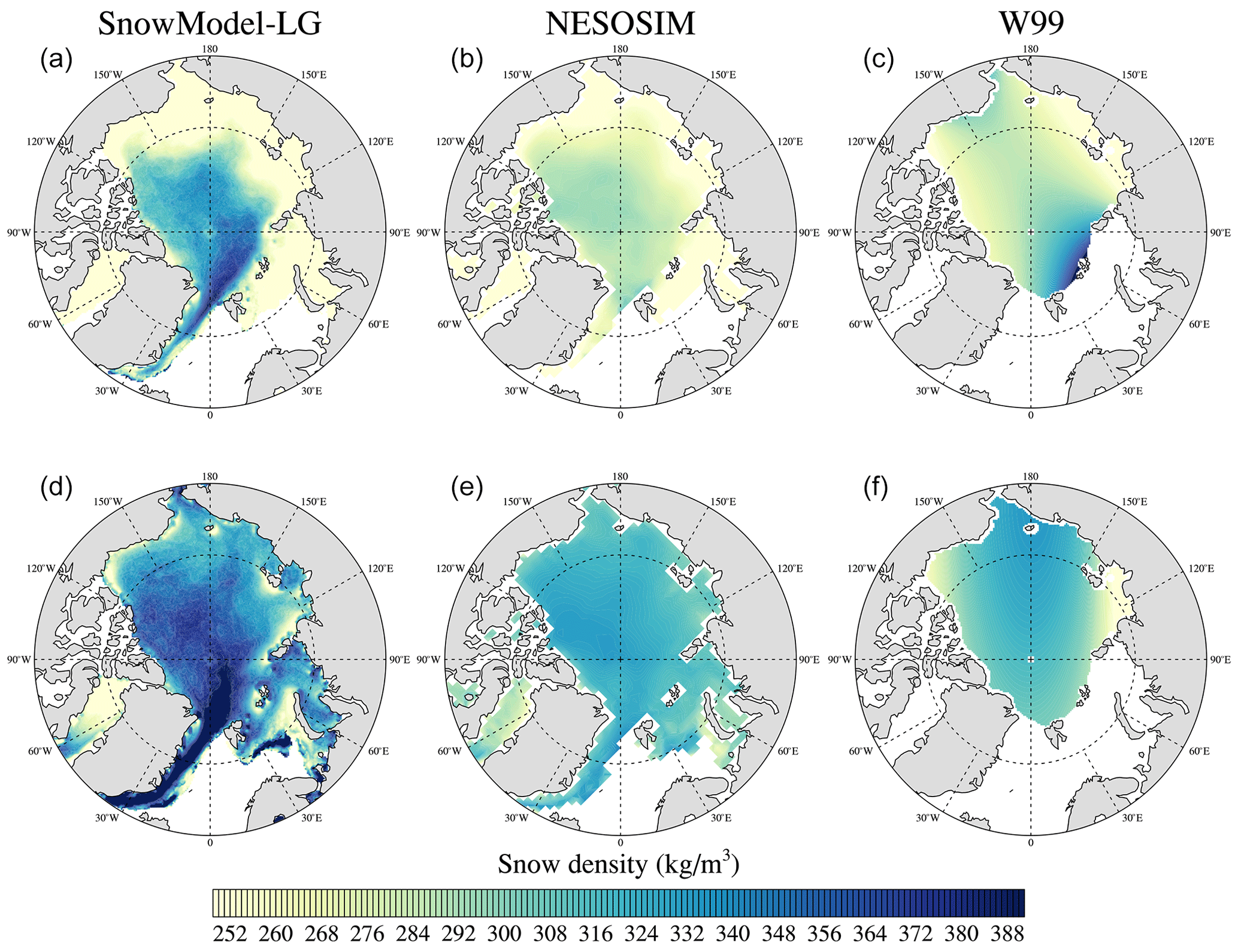
Figure 10 Mean snow density (units: kg m⁻³) according to SnowModel-LG, NESOSIM and W99 in November (a–c) and the next April (d–f) since 2000.

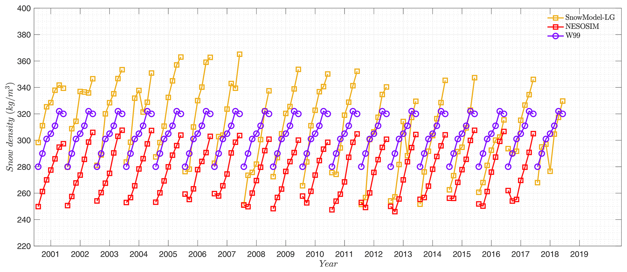
Time series of wintertime mean snow density within the Arctic basin in SnowModel-LG, NESOSIM and W99 are summarized in Fig. 11. Both SnowModel-LG and NESOSIM show an increase in snow density into the winter, which is consistent with W99. However, snow density in SnowModel-LG is consistently higher than that of NESOSIM, with more pronounced differences at the end of winter; W99 falls between the two estimates at 320 kg m⁻³. Seasonally, SnowModel-LG densities increase more from October to April than in NESOSIM and W99. Neither the NESOSIM nor SnowModel-LG densities suggest any long-term changes in snow density, yet SnowModel-LG shows considerable interannual variability of spring and winter snow density, which is not present in NESOSIM or W99.

Figure 11 Time series of mean snow density (units: kg m⁻³) within Arctic basin (common region in Fig. 1) comparison in SnowModel-LG, NESOSIM and W99 since 2000.

4 Comparison of snow depth products against observations

In this section, we compare the snow depth products against the observational data sets. Since snow depth data from OIB play an important role in the development of some of the snow products, the comparison and validation potentially suffer from the problem of data dependency. This applies to both reanalysis-based snow reconstructions and the satellite-retrieved snow depth fields. Buoy-based comparisons are free from the data dependency problem, yet the limited local spatial coverage of buoys hinders direct comparisons with the products in study, which are all on much coarser spatial scales (>10 km). Therefore, after the intercomparisons we discuss the complexities in validating different snow products and observations with in situ and airborne measurements in Sect. 4.3.

4.1 Comparison against OIB

We assess the snow products against four different OIB snow depth products. We first compare OIB and snow products after gridding both to a common 100×100 km grid and by evaluating the monthly averages in 2014 and 2015. Results are shown in Fig. 12 and Table 2. Taking the quicklook product as an example, there are on average 1300 OIB 40 m mean measurement samples per grid cell. It should be noted that snow depths from DuST, PMW Bremen and DMI are directly fitted against OIB snow depths, and as a result, these data show significantly correlations (over 0.36 for PMW DMI) with OIB as shown in Table 2. Therefore, we do not consider this a suitable validation (or comparison) for these products. For the PMW DMI product, however, OIB data from the period from March 2014–2015 were not used during model development, and hence we have more confidence in the high correlation observed. Except for NESOSIM and UW, the other reanalysis-based products are also to some extent indirectly tuned by OIB snow depths in some years. Overall, all products show reasonably high correlations with the different OIB snow estimates except for UW, which only shows a slight correlation with some versions of the OIB data.

Figure 12 March and April comparison (only April in UW and March in DESS) between four monthly OIB products (quicklook in blue, GSFC in green, JPL in red and SRLD in purple) and all snow products monthly on a 100 km grid for the period of 2014 and 2015. Lines are best linear fits. Numbers in left corners indicate the valid count in the linear fitting.

Table 2 R² (in bold), RMSE (left in bracket, units: cm) and NRMSE (right in bracket) of various average monthly snow depth products in comparison with four OIB snow depth products, using a 100×100 km monthly comparison.

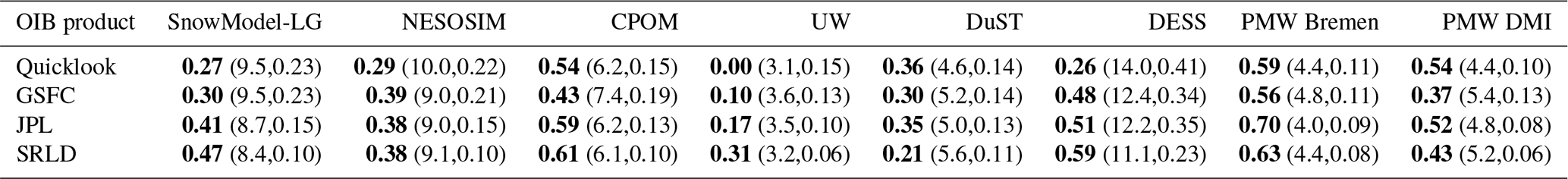
It should be noted that OIB snow depth is itself a derived product, and thus caution is warranted when interpreting the results of the comparison with snow products. In fact, a strong dependence of our validation results on the specific OIB data product is evident by the different linear fitting slopes shown in Fig. 12, as well as the R² values, RMSE and normalized RMSE (NRMSE: $\text{RMSE}/(max-min)$) in Table 2. The fit is best for the PMW Bremen and PMW DMI data, followed by the CPOM and DESS products, though this depends on the choice of OIB data set used for evaluation. For example, CPOM performs best against SRLD (R²=0.61) and worst against GSFC (R²=0.43); DESS also performs best against SRLD (R²=0.59) but worst against quicklook (R²=0.26). SnowModel-LG and NESOSIM have similar R² ranging from a low R² of 0.27 and 0.29, respectively, against the quicklook product to a high of 0.47 (SnowModel-LG vs. SRLD) and 0.39 (NESOSIM vs. GSFC). The UW snow product, on the other hand, performs poorly against all OIB snow depth estimates (maximum R² of 0.31 with SRLD). Among all non-directly OIB-fitted snow products (SnowModel-LG, CPOM, DESS, UW and NESOSIM), RMSE in CPOM is the lowest, while in DESS the RMSE is over 10 cm. The distribution/variability in UW is narrow compared with other products related to the lack of spatial variability of snow depth across the basin.

In order to avoid biases introduced by temporal and spatial averaging and interpolation during the validation, we also carry out the comparison for each of the data products on their native grids and native temporal resolution (Fig. S4). In contrast to the coarser-resolution comparisons shown in Fig. 12 and Table 2, more outliers, lower R² values and larger RMSEs are evident in these native-spatial–temporal-resolution comparisons. The comparison results still depend on the choice of OIB data product, and in some instances the statistical correlation improves. There is still no significant correlation between UW snow depths and those from OIB, but the overall RMSE is the lowest recorded at less than 4.0 cm. PMW DMI has the lowest NRMSE, followed closely by all other snow products, with the largest NRMSE in DESS. All snow products except NESOSIM and UW show higher R² under spatial coarser resolution compared to Fig. 12, Fig. S4 and Table S3. The comparisons between monthly and daily scale estimates suggests that temporal resolution has little influence on OIB comparisons, since there are only small changes in R² and RMSE, without significant differences. However, spatial resolution does impact the statistical fits, which is related to the lack of representation between OIB and these products at the coarse scale of 100 km (discussed further in Sect. 4.3).

Given the potential data dependency problem and the sensitivity to the specific OIB data set, it is not possible to conclude which snow product performs best. Snow products that have been produced through tuning with OIB data show higher R² and smaller RMSEs. The PMW DMI product performs best, despite not being tuned with OIB data for the time period to which it is compared. The outlier is the UW product. In summary, there is a need for a consensus as to which OIB data products are the most accurate and also for further independent observations to compare against the various pan-Arctic snow products currently available to the science community.

4.2 Comparison with buoy data

We further explore how well the snow products represent the mean state of small-scale snow depth on Arctic sea ice by comparing against CRREL IMBs and AWI snow buoys. As discussed in Sect. 2.1.1, 86 buoy tracks (58 tracks are from CRREL and 28 tracks are from AWI) were processed from 2000 to 2017 (Table S1). Scatterplots in Fig. 13 between monthly mean (March and April) buoy snow depths and those from the various products are based on their native spatial resolution. DuST is excluded due to a lack of buoy samples in its more limited spatial coverage. Despite some statistically significant correlations, the correlations are all very low, with slopes close to 0. The highest correlation among the products is 0.16 for DESS. The PMW Bremen and PMW DMI products show essentially no variability/spread compared to the buoy data.

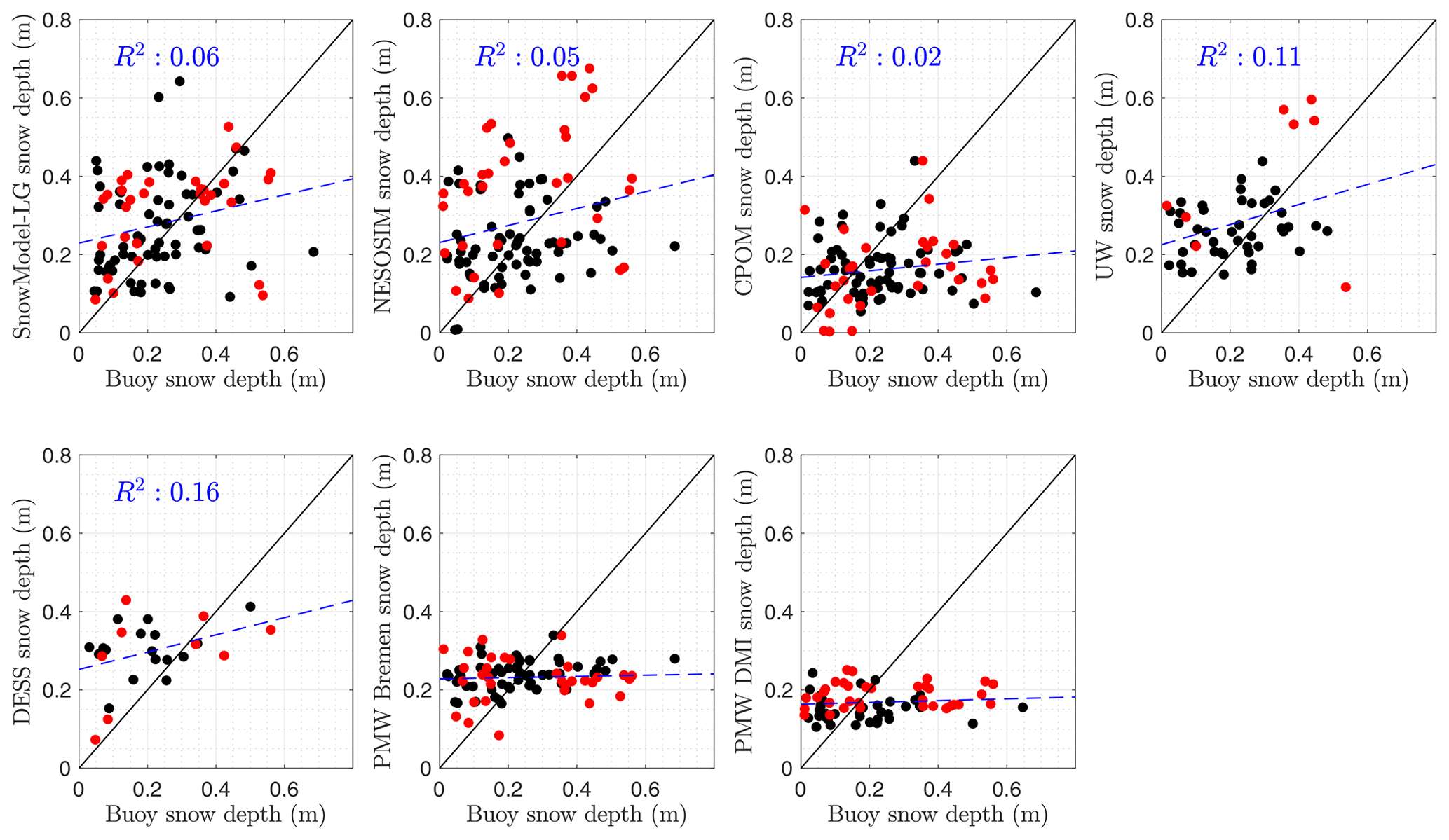
Figure 13 Comparison of average March and/or April snow depth in snow products in native spatial resolution versus the AWI (red dots) and IMBs (black dots) buoys. All significant correlation (R²) values are given in blue.

Next, we focus on temporal evolution as we do not expect the local-scale point measurements of the IMBs and snow buoys to match with the coarse spatial scale of the data products. We compare snow depth differences in the products along the buoys' drifting tracks against the accompanied snow accumulation measured by buoys during winter (Fig. S5). Specifically, the three daily-resolution products (SnowModel-LG, NESOSIM and CPOM) are interpolated onto daily geolocations of the buoys. Only buoys with valid measurements from October until the following February are considered. Snow accumulation is then calculated by subtracting the mean snow depth within the first 7 d and that in the last 7 d. None of these products show significant correlation with buoy accumulation because several outliers weaken the overall correlation. Based on Stroeve et al. (2020), good correlations are witnessed between SnowModel-LG and buoy data using the buoy location in each integration step. Therefore, the lack of correlation we observe may be due to large discrepancies in trajectories determined from the ice drift products and from buoys, especially after a long-term integration.

In general, the comparison with snow depth measurements from buoys highlights two important limitations of these sorts of comparisons. First, pronounced representation issues are present when comparing point measurements to coarse-resolution products despite buoys being intentionally deployed to represent the adjacent areas and despite the fact that they potentially traverse large geospatial ranges. Second, sea ice drift is a major factor in determining the uncertainty of snow depth estimations during the numerical integration of reanalysis-based approaches.

4.3 Study of representation issues

Comparison and validation of snow depth products with observations of vastly different spatial resolutions and coverage are complex. For OIB, although the ground tracks cover large regions, the aggregate footprint size is small. For example, an average of 1300 OIB samples are used to compute the 100×100 km cell-mean snow depth and the aggregate area is about 0.6 km², which is 0.006 % of the 100 km cell. The same spatial aliasing situation has long existed in sea ice thickness (Geiger et al., 2015), where the different instrument footprint sizes bring about artificial modes in thickness distribution. However, here the spatial coverage of OIB mitigates this problem, by introducing large-scale variability in computing the cell-mean values of snow depth. For comparison, buoy measurements are the extreme case of limited representation for products with coarse resolution. Although the absolute error for each buoy measurement is low, the practice of using it for validation purposes should be scrutinized.

In order to study the effect of limited spatial coverage on validation, we utilized an OIB data set to simulate various spatial grid spacings of products that can be used for snow depth validation, including the extreme case of point measurements (e.g., buoys). Specifically, we divide OIB scans into segments of about 37.5 km, which is the typical resolution of the snow products evaluated in the study. The mean snow depths from all OIB measurements within each segment are computed and treated as the true snow depth (hereinafter referred to as Hs), which is then used as the snow depth measurement to be validated. Re-sampling, that is multiple selections from samples, of the OIB measurement in each segment is carried out, in order to simulate the various observations with limited coverage. By studying the behaviors of fitting snow depth (Hs) values to samples, we observe the change in the slopes and qualities of the statistical fits. Three sampling strategies are designed: (I) random re-sampling, for which 40 OIB samples are randomly chosen within the segment region and used to compute the mean Hs; (II) segment-based re-sampling, for which a local OIB segment track with 40 consecutive samples is chosen and used to compute mean Hs; and (III) single sample, for which a single OIB Hs measurement is chosen to represent the locally measured snow depth. Strategy III essentially mimics a buoy observation in 1 d within typical passive microwave satellite spatial resolution (i.e., limited spatial coverage). Specifically, in order to further increase the validity of strategy III for mimicking buoy measurements, we make sure that the thickness of the random single sample in strategy III is within 1 standard deviation of the mode of the OIB ice thickness distribution.

Figure 14 The study with OIB on the effects of sampling strategy for observations. Snow distribution within typical region (a) under different sampling method embedded with schematic on different strategies deployment: original OIB measurements (black), 40 consecutive OIB re-sampling (strategy II: blue) and 40 random OIB re-sampling (strategy I: red). Mean snow depth is shown by dashed lines. Typical fitting (b) between cell mean and a single sample snow depth for all regions, with fitting line in purple. Overall distribution of slopes (c) in three re-sampling strategies, fitting between OIB cell mean and 40 random OIB samples (strategy I), between OIB cell mean and 40 consecutive samples (strategy II), and between OIB cell mean and single sample within 1σ of the mode of the ice thickness (strategy III: black).

Figure 14a shows the snow depth distribution from strategy I (red lines) and strategy II (blue lines) for an example segment, in order to demonstrate the simulation strategies. A typical case of the fitting in strategy III is shown in Fig. 14b, with each dot representing a local region of 37.5 km. After extracting and averaging the sample in different strategies, snow distribution is much narrower in strategy I and II than in the original measurements, especially in random re-sampling. Using Monte Carlo simulations with re-sampling, we compute the distribution of fitting slopes for the three strategies, shown in Fig. 14c. In strategy I (random re-sampling), due to the small number of OIB samples chosen (40 samples), the slopes of the linear fitting lines are lower than 1 (around 0.91). This indicates that even if there is overall good coverage of the measurements, the limited footprint still causes the fitting lines to flatten. If we limit the measurement of Hs to a local segment (40 consecutive samples: strategy II), the slopes drop to about 0.73, which indicates that the limited representation of the local segment to regional variations further affects the validations. This is also in direct contrast with strategy I. When we further limit the comparison to a single OIB sample (strategy III), the slopes further decrease to around 0.24. It is important to note that, although the fitted lines are very flat (an example in Fig. 14b), the fittings are all statistically significant.

This result agrees with the buoy validation results in Sect. 4.2, where the fitted slope between snow products and buoy data (Fig. 13) is considerably flatter when compared with the results involving OIB observations, as a result of both large aggregate footprint and wider spatial coverage of OIB. Yet, the study with OIB data suggests that the product validation with buoy data should yield statistically significant correlations. This result also indicates that when tuning the prognostic/statistical models against airborne or in situ measurements for reconstructing snow, the uncertainty concerning limited representation should be addressed in order to avoid over-fitting. The systematic study of uncertainty quantification for limited representation is beyond the scope of this paper and planned as future work.

5 Summary and outlook

This paper offers a detailed assessment of current snow products over sea ice. Although general consistency in snow structure is witnessed among the products in terms of deeper snow over perennial ice, regionally large spatial and temporal discrepancies do occur. Further, the magnitude of seasonal snow accumulation differs, as do long-term trends. Among the products evaluated, UW and PMW DMI provide the upper and lower extremes of snow volume/depth at the end of the freezing season. Wintertime snow accumulation is overall less than in the W99 climatology and is postponed towards springtime in the reanalysis-based products. On the other hand, the satellite-derived DuST product does not exhibit a distinct wintertime snow accumulation. Interannual variability of precipitation in the majority of reanalysis-based products was found to be consistent (Barrett et al., 2020), and thus we may have expected the reanalysis-based snow depth to share similar interannual variability in snow depth. However, different methods for accumulating the precipitation in the reanalysis, as well as how that precipitation is redistributed within the Arctic basin under ice motion, leads to pronounced differences among the reanalysis-based products. The March and/or April interannual variability for all snow products was about half that previously estimated by W99 (3.0 cm vs. 6.1 cm). Furthermore, none of the current snow products display a trend in overall snow depth since 2000, although they all suggest significantly thinner snow in spring than found in the climatologies. Over a longer time period, however, several of the reanalysis-based snow products do show statistically significant trends towards thinner snow.

We further compared each product against OIB and buoy observations. All snow reconstructions demonstrate significant correlation with OIB observations, except for UW, which only shows a slight correlation with some versions of the OIB data. Correlations are lower when compared against buoy measurements (no significant correlation in PMW Bremen and PMW DMI), with the highest correlation of 0.4 in DESS. We suggest that poor correlations are at least in part caused by representation issues when trying to validate coarse observations against finer-resolution measurements. More effort is required to simulate how snow accumulates locally since currently no product has the ability to model snow depth at local spatial scales, as captured by observational platforms such as buoys. For the reanalysis-based products, improvement in the ice drifting algorithm and snow redistribution parameterization may result in more accurate representation of snow distribution. Based on the results, we pick SnowModel-LG, NESOSIM, CPOM and DESS as the products with the highest consistency. While we cannot reach conclusive results on which snow product best represents the true snow depth, we emphasize the importance of further coordinated intercomparisons and call for community effort to collect more independent observations for snow over sea ice.

Despite its importance for polar climate studies and sea ice altimetry, the snow cover on sea ice remains a scarcely observed parameter. Airborne surveys such as OIB provide a good trade-off between spatial resolution and coverage, yielding one of the richest snow depth observations for the polar regions. Although it is a derived product, OIB snow depth has become a major reference for model tuning, as well as the benchmark for many snow depth reconstruction products. Therefore, although the comparisons with OIB snow depth differ among the products (Sect. 4.1), there remain inherent limitations regarding data dependency. Given the status quo of limited snow depth products as reference data sets, more independent observations are required. The problems associated with validation and data dependency would be avoided by using separate training and testing data sets (such as subsets of OIB snow depth data) for the model tuning of snow reconstructions.

Due to the resolution differences of the various snow depth products, spatial and temporal representation issues need to be explored further to facilitate detailed comparison and validation. This is especially true when validating coarse-spatial-resolution data with local snow depth measurements such as buoy or a single OIB sample (Sect. 4). In order to address these issues, the multi-scale characteristics of the snow should be studied in a systematic manner, including (1) its distribution and interaction with sea ice (Xu et al., 2020) and (2) the scaling properties for a wide range of measurement footprints, including in situ measurements with snow probes and snow stakes (footprint <0.1 m²), airborne measurements (≈100 m²), and typical satellite passive microwave imagers (100–1000 km²). Uncertainty quantification can then be carried out and incorporated in the development of new snow remote sensing techniques, as well as product intercomparison and validations.

With climate change and Arctic warming, the snow cover on sea ice has undergone drastic changes. A longer melting season, later freeze-up and shrinking of the perennial sea ice cover have resulted in an overall thinning of the snow cover (Sect. 3.1). However, the polar hydrological processes have become more pronounced with warming, with stronger and more frequent polar storms inducing more snowfall (Webster et al., 2019). In addition to these competing factors influencing the total amount of snow on Arctic sea ice, the snow stratigraphy and potential changes are a challenge for both remote sensing and modeling of the snow cover. With the combined factors of more snowfall and thinner sea ice, the resulting snow–ice formation causes changes in the thermodynamic and radiometric properties of the snow cover, as witnessed in N-ICE2015 (Gallet et al., 2017; Merkouriadi et al., 2017). In addition, the repeated intrusions of warm air causes snow stratigraphy changes and even thawing–refreezing cycles, bringing challenges to both airborne and satellite remote sensing of the sea ice and snow cover. Furthermore, the long-term increase in Arctic precipitation is projected to continue in the future decades, with potential transition in the phase of precipitation (Bintanja and Selten, 2014). The complex processes involving snow stratigraphy pose further challenges for the modeling of active/passive radiometry of snow and sea ice, as well as that of prognostic modeling of snow over sea ice.

Current and future in situ and satellite campaigns contribute to an ever-growing and enriching catalogue for snow and sea ice observations. In situ campaigns, such as MOSAiC, provide annual, process-level studies of the atmosphere–ice–ocean coupled system for the Arctic. Novel satellite campaigns such as the multi-frequency radar altimeter CRISTAL (Kern et al., 2020) will provide unique capabilities for snow depth measurement and sea ice altimetry. The abundance of the methodologies and techniques that are investigated in this study shows that there is general consistency among the products derived by both numerical and satellite-based approaches, and snow on Arctic sea ice is significantly thinner against observations from the last century. However, some spatial–temporal differences among these products call for more attention for more independent snow observations as well as modeling improvements.