the Creative Commons Attribution 4.0 License.
the Creative Commons Attribution 4.0 License.
 | 27 Nov 2020
Using ICESat-2 and Operation IceBridge altimetry for supraglacial lake depth retrievals
Mark Flanner
Kelly M. Brunt
Helen Amanda Fricker
Alex Gardner
Supraglacial lakes and melt ponds occur in the ablation zones of Antarctica and Greenland during the summer months. Detection of lake extent, depth, and temporal evolution is important for understanding glacier dynamics. Previous remote sensing observations of lake depth are limited to estimates from passive satellite imagery, which has inherent uncertainties, and there is little ground truth available. In this study, we use laser altimetry data from the Ice, Cloud, and land Elevation Satellite-2 (ICESat-2) over the Antarctic and Greenland ablation zones and the Airborne Topographic Mapper (ATM) for Hiawatha Glacier (Greenland) to demonstrate retrievals of supraglacial lake depth. Using an algorithm to separate lake surfaces and beds, we present case studies for 12 supraglacial lakes with the ATM lidar and 12 lakes with ICESat-2. Both lidars reliably detect bottom returns for lake beds as deep as 7 m. Lake bed uncertainties for these retrievals are 0.05–0.20 m for ATM and 0.12–0.80 m for ICESat-2, with the highest uncertainties observed for lakes deeper than 4 m. The bimodal nature of lake returns means that high-confidence photons are often insufficient to fully profile lakes, so lower confidence and buffer photons are required to view the lake bed. Despite challenges in automation, the altimeter results are promising, and we expect them to serve as a benchmark for future studies of surface meltwater depths.
- Article
(2958 KB) - Full-text XML
- BibTeX
- EndNote


The ice sheets of Antarctica and Greenland modulate rates of sea level rise, contributing 14.0 ± 2.0 mm (Antarctica) and 13.7 ± 1.1 mm (Greenland) since 1979 (Mouginot et al., 2019; Rignot et al., 2019). Current trends indicate greater melt in the coming decades, leading to the contributions from both ice sheets to overtake the contribution of thermal expansion to sea level rise (Vaughan et al., 2013). Meltwater plays vital roles in ice sheet evolution (e.g., van den Broeke et al., 2016), including aggregation on ice sheets as supraglacial lakes, many of which are several meters deep (Echelmeyer et al., 1991). When unfrozen, these lakes exhibit a lower albedo than that of the surrounding ice, allowing them to absorb more incoming solar radiation and melt ice more efficiently, thus generating a positive feedback (Curry et al., 1996). Supraglacial lakes are significant reservoirs of latent heat (Humphrey et al., 2012), and their spectral emissivity in the infrared (IR) spectrum also differs from bare ice (Chen et al., 2014; Huang et al., 2018), which can lead to potentially significant impacts on the surface energy balance of ice sheets.
A substantial portion of meltwater eventually drains into supraglacial streams or moulins (drainage channels), where it can flow to the ice bed (Banwell et al., 2012; Catania et al., 2008; Selmes et al., 2011). During catastrophic lake drainage events, meltwater penetration into the ice can also lead to hydrofracture, a mechanism through which meltwater facilitates full ice fracture as a result of the stresses induced by the density contrast between liquid water and ice (Das et al., 2008). Meltwater injection to the bed can also modify basal water pressures which in turn modify the resistance to ice flow and thus can impact sliding velocity and ice discharge. (Parizek and Alley, 2004; Zwally et al., 2002). Hydrofracture can lead to significant ice loss for outlet glaciers and ice shelves (Banwell et al., 2013). Current observations and modeling efforts indicate a propagation of supraglacial lakes farther inland as the climate warms (Howat et al., 2013; Leeson et al., 2015; Lüthje et al., 2006), raising further concerns for accelerated mass loss. For these reasons, knowledge of supraglacial lakes is important for our understanding of ice sheet evolution.
Previous studies developed techniques for detecting supraglacial lakes and retrieving depth, areal coverage, and volume. In situ observations employed sonar and radiometers to approximate lake depth and albedo (Box and Ski, 2007; Tedesco and Steiner, 2011). However, the harsh conditions of Antarctica and Greenland, the transience of meltwater, and the sheer size of the ice sheet ablation zones restrict the potential for extensive in situ measurements, encouraging lake depth and areal coverage estimates from passive remote sensing data such as Landsat-8, MODIS, and Sentinel-2 A/B. Supraglacial water is darker than surrounding ice in the visible and IR bands, allowing the use of band ratios between blue and red reflectance (Stumpf et al., 2003). The normalized water difference index (NWDI) and dynamic thresholding techniques have also been considered for lake detection (Fitzpatrick et al., 2014; Liang et al., 2012; Moussavi et al., 2016; Pope, 2016; Williamson et al., 2017; Moussavi et al., 2020). Other methods implemented radiative transfer models (Georgiou et al., 2009) or positive-degree-day models (McMillan et al., 2007) to estimate lake albedo and meltwater volume. By comparing surface reflectance data of supraglacial water to that of ice and optically deep water, empirical relationships have been derived to approximate lake depth (Philpot, 1989; Sneed and Hamilton, 2007).
Image-based empirical techniques rely on approximations of lake bed albedo and an attenuation parameter, both of which are subject to uncertainties from lake heterogeneity and cloud cover (Morassutti and Ledrew, 1996). Furthermore, Pope et al. (2016) found that band ratios were insensitive to lakes deeper than 5 m, leading to errors that may exceed 1 m. Parameter fitting in the empirical equations requires supplementary depth retrievals, often from in situ sources. More accurate methods for supraglacial lake detection are needed to improve image-based estimates.
In September 2018, the Ice, Clouds, and land Elevation Satellite-2 (ICESat-2) was launched with the primary objective of obtaining laser altimetry measurements of the polar regions (Abdalati et al., 2010; Markus et al., 2017; Neumann et al., 2019b). Observations using the Airborne Topographic Mapper (ATM) and Multiple Altimeter Beam Experimental Lidar (MABEL) indicated the potential for shallow water profiling with laser altimetry (Brock et al., 2002; Brunt et al., 2016; Jasinski et al., 2016), and ICESat-2 applications were recently demonstrated by Ma et al. (2019) and Parrish et al. (2019). In this study, we identify test cases from ICESat-2 and ATM altimetry data and use these pilot cases to develop an algorithm for detecting supraglacial lakes and retrieving lake depth. The algorithm is designed as a semiautomatic method to find supraglacial lakes within select altimetry granules.
2.1 ICESat-2
ICESat-2 is a polar-orbiting satellite with an inclination of 92∘ that carries the Advanced Topographic Laser Altimeter System (ATLAS), a 532 nm micro-pulse laser that is split into six distinct beams with names based on the ground track: GT1L/R, GT2L/R, and GT3L/R. The beams are configured in pairs with a 90 m separation between beams within a beam pair and 3.3 km between pairs. With an operational altitude of ∼ 500 km and a 10 kHz pulse repetition rate, ICESat-2 records a unique laser pulse approximately every 0.7 m along-track over a 91 d repeat cycle.
The ATLAS product used here is the ATL03 Global Geolocated Photon Data V002 (Neumann et al., 2019a), which consists of retrieved photons tagged with latitude, longitude, received time, and elevation. Each photon pulse also carries a classification as either signal or background (noise). The differentiation between signal and background is performed using a statistical algorithm outlined by Neumann et al. (2019b). Signal photons are further classified by confidence level, such that photons labeled as “high confidence” are most likely to originate from the surface. Generally, cloudy or variable profiles exhibit “medium/low confidence” or noise photons, whereas low-slope surfaces, such as water and ice sheets, result in more high-confidence photons (Neumann et al., 2019b). In thin layers of water, high-confidence photons are observed from both the water surface and the underlying ice.
Our study focused on the central strong beam (GT2L), as the number of lakes was deemed sufficient for our purposes. While we recognize that the other strong beams could be useful for depth retrievals, we did not consider them here. We speculate that the weak beams may avoid issues with multiple scattering and specular reflection, but their power is too low to reliably detect lakes deeper than 4 m. Ground-based validation by Brunt et al. (2019b) indicates an accuracy of <5 cm in ATL03 photons over ice sheet interiors. The use of medium, low, and “buffer” photons slightly decreases measurement precision, but a less truncated transmit pulse gives better agreement with ATL06 and ground-based data (Brunt et al., 2019b).
2.2 Airborne Topographic Mapper
The Operation IceBridge (OIB) campaign was designed to fill the gap in polar altimetry between ICESat and ICESat-2. Its scientific payload included the Airborne Topographic Mapper, a 532 nm lidar that has been used for ice sheet and shallow water measurements since 1993. The ATM lidar conically scans at 20 Hz, providing a 400 m swath width along-track (Brock et al., 2002; Krabill et al., 2002). The ATM Level-1B Elevation and Return Strength (ILATM1B) product converts analog waveforms into a geolocated elevation product to emulate ATLAS data (Studinger, 2013). Although it lacks a statistical confidence definition, ATM applies a centroid model to digitized waveforms to retrieve high-confidence photons. Brunt et al. (2019a) found that ATM errors were −9.5 to 3.6 cm relative to ground-based measurements. Here, the ATM results presented serve as a proof of concept for the lake detection algorithm.
3.1 Lake detection
Supraglacial lake surfaces are much flatter than surrounding terrain. We thus performed topography checks with the expectations that (i) lake surfaces would be identifiable in photon histograms and (ii) lake beds may be found via statistical inference in the region of the lake surface. To simplify the identification of lake features, we separated them into two arrays: one for the surface and one for the bed, which we refer to as “lake surface–bed separation” (LSBS). For both lidars, the procedure for separation was identical and is as follows (see Fig. 1 for a schematic view).
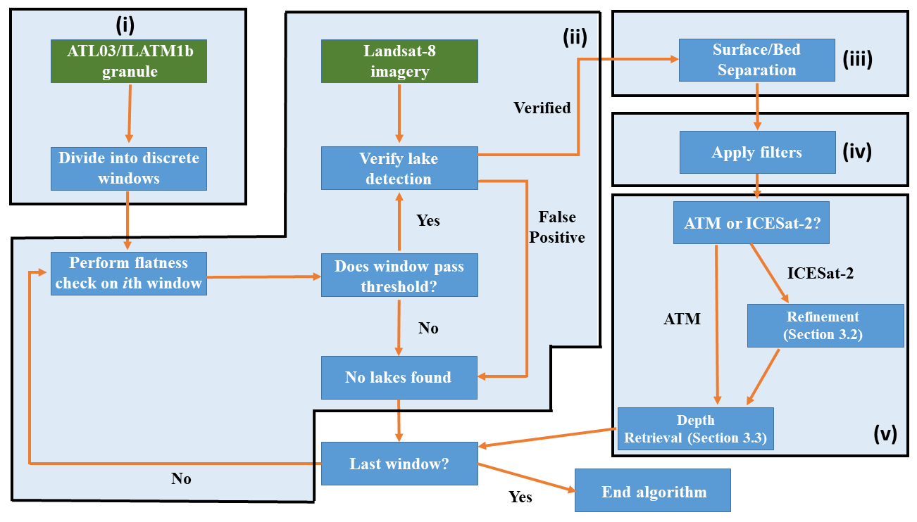
- i.
We divided each data granule into discrete along-track windows to reduce the data volume to ∼ 104–105 photons per window. This photon count is equivalent to ∼ 1–10 km in the along-track distance for ICESat-2 and ∼ 0.15–1.5 km for ATM. If a supraglacial lake appeared on the edge of the window, the window size was adjusted to include the full observed water feature.
- ii.
Each data window was binned into elevation-based histograms. We assumed that the lake surface dominates the total bin count within each window of photons. We check the flatness of the window by computing the standard deviation (σ) of high-confidence signal photons within the upper 85th percentile of bin count. We define a “flat” surface for regions where σ≤0.05 m for ATL03 data and ≤ 0.02 m for ILATM1B data. We selected these values by comparing the flatness of lake surfaces to that of surrounding ice topography. If data were within the appropriate flatness threshold, they were verified as a lake surface using Landsat-8 OLI imagery. This step was included to filter non-glacial features, such as ocean or fjords.
- iii.
If the satellite image(s) confirmed the presence of a lake, the data were assigned to a new array for the height of the lake surface (hsfc). The horizontal extent of the lake surface served as a constraint for where the lake bottom data could be defined. Within these horizontal bounds, photons were defined as a lake bottom if they satisfied the condition , where σsfc is the standard deviation of lake surface photons. The constraints a and b were derived through trial and error, such that a=1.0(1.8) and b=0.5(0.75) for ICESat-2 (ATM). We set these constraints to reduce the impacts of multiple scattering and specular reflection on depth estimates. If these conditions were met, then the data were placed in an array for the height of the lake bottom, hbtm.
- iv.
A series of filters were applied to improve surface–bed estimates. For ICESat-2, lakes shallower than 1.3 m or smaller than 200 m in horizontal extent were considered too noisy or ill-defined for further analysis (see Sect. 5.2 for more details). To remove water bodies with deep bed returns (e.g., oceans or fjords) or with no bed returns, the algorithm counted the number of bed photons present for both lidars. If the number of bed photons was very small (100 or less), then the scene was marked as a probable false positive.
- v.
If the data were obtained from ICESat-2, then we followed a photon refinement routine that is described in more detail in Sect. 3.2. Calculations for lake depth were then performed for both ATM and ICESat-2 retrievals and corrected for refraction (Sect. 3.3).
3.2 ATL03 refinement
The above steps were sufficient to obtain lake profiles within the ATM data, but melt lake bottoms observed by ICESat-2 were significantly noisier as a consequence of higher background (noise) photon rates. After the initial LSBS procedure, we manually assessed bed estimates for each lake. For lakes that did not pass qualitative assessment, we adopted photon refinement procedures initially used for the ATL06 surface-finding algorithm (Smith et al., 2019). In short, ATL03 photon aggregates within overlapping 40 m segments were used to estimate lake surfaces and beds with greater precision via least-squares linear fitting applied to the aggregates. These linear fits were used to approximate a window of acceptable surface or bed photons for every 20 m along-track. A more detailed description of the ATL06 algorithm is given in Smith et al. (2019).
The linear regression in ATL06 accounts for all ATL03 photons (background or signal), and the technique performs a background-corrected spread estimate to narrow the range for acceptable photons. This is an iterative scheme; the refinement process repeats its acceptable photon filter until no photons are removed. As a consequence, the ATL06 algorithm assumes a single returning surface, so over a melt lake it will compute a height for either the lake bottom or the lake surface, depending on their return strengths.
The condition for acceptable surface photons in ATL06 is given by
Within a 40 m photon segment, r is the residual of a photon relative to the linear regression, rmed is the median residual, and Hw is window height. The height of the window is taken as the maximum of the observed photon spread, the window height (if any), and 3 m, and photons within the window range are defined as the surface. The LSBS algorithm follows a similar procedure, but the flatness of the lake surface and relatively low photon density of the corresponding beds rendered iteration unnecessary. The lake bed is then defined as photons not within the window and below the surface. In other terms, lake bed photons satisfy the conditions
As with the initial guess, the lake bottom was only defined within the horizontal bounds of the lake surface, and the improved guesses were assigned to hsfc and hbtm.
As a final adjustment to lake photons, we applied a refraction correction algorithm to account for slowing down of light as it enters water. The correction follows the methods utilized by Parrish et al. (2019) by approximating refractive biases as a function of depth and beam elevation angle. The center strong beam for ICESat-2 is near the nadir, so the horizontal offset was determined to be small relative to the size of lakes (∼ 3 cm, far below the horizontal geolocation uncertainty for ICESat-2). However, vertical offsets of 1 m or more were found for lakes ≥4 m in depth, necessitating the use of refraction correction.
3.3 Lake depth and extent estimations
Once we obtained hsfc and hbtm, lake depth from the altimeter signal (zs) was estimated using
where and represent the moving mean of the surface elevation and the bottom elevation, respectively. The moving mean was used to account for signal attenuation and scattering at the lake bottom, a problem most evident for ICESat-2 retrievals.
For deep or inhomogeneous lakes, attenuation of photon energy in water resulted in fewer signal photons observed at lake bottoms (Fig. 4). In these situations, we fitted polynomial or spline fits to all lake profiles with bounds at the lake edges. Lakes observed by ATM typically featured “bowl” shapes and attenuation at the deepest parts, so third-order polynomials were sufficient. In ICESat-2 data, the retrieved lake beds showed greater complexity, so we tested polynomial fits and splines on a case-by-case basis. Lake depths approximated with curve fitting were denoted as zp. We compare zs and zp over lakes with well-defined bottoms, and we show in Sect. 4 that the two generally agree to within 0.88 m.
To test the limits of the algorithm relative to lake size, we utilized the great-circle formula (ATM) or predefined along-track distance (ICESat-2) to approximate along-track extent L. We acknowledge the desire to retrieve lake volume from laser altimetry, but we leave the development of such an algorithm for a future study. For example, depth retrievals from ICESat-2 could potentially be combined with lake radius and shape estimations determined from visible satellite imagery to derive water volume.
3.4 Case study locations
We present cases over the Amery Ice Shelf on 2 January, 2019 (ICESat-2 Track 0081; 68.271–73.798∘ S, 63.057–78.620∘ E), the western Greenland ablation zone for 17 June 2019 (ICESat-2 Track 1222; 66.575–69.582∘ N, 48.284–49.239∘ W), and Hiawatha Glacier on 19 July 2017 (ATM; 77.780–79.3119∘ N, 65.279–67.484∘ W) (Fig. 2). Comparisons between Landsat-8 imagery and ICESat-2/OIB flight tracks confirmed supraglacial lake overpasses for study. In spring 2019, an early onset of the Arctic melt season resulted in both ICESat-2 and Operation IceBridge surveying supraglacial lakes near Jakobshavn Isbræ in May. However, there were no lakes sampled at the time by both ICESat-2 and OIB.
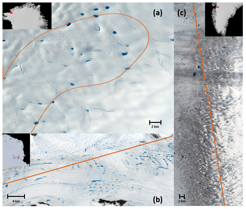
Figure 2True-color Landsat-8 composites of Hiawatha Glacier on 18 July 2017 (a), the Amery Ice Shelf on 1 January 2019 (b), and the western Greenland ablation zone on 17 June 2019 (c). Flight tracks for Operation IceBridge (a) and ICESat-2 (b, c) are shown in dotted orange.
We detected 12 melt lakes with sufficient bed returns from the ATM data and 16 potential melt lake surfaces overall. The melt lake profiles are shown in Fig. 3, with maximum depths of 0.98–7.38 m and extents of 180–730 m. The algorithm reliably distinguishes between lake surfaces and the surrounding ice terrain. The mean spread among lake surface photons is 0.0087 m, or well within the flatness threshold of 0.02 m. Lake bottoms are well-defined when ds<8 m. Lake bottoms deeper than 8 m exhibit fewer signal returns, for the associated return signal is below the threshold required to be digitized (Martin et al., 2012). The average depth estimate for the lakes in Fig. 3 was 1.95 m (Table 1), and lakes at this depth typically featured adequate bed returns. In deeper lakes, the polynomial estimate produced reasonable guesses for the lake bed location, with the most effective fitting seen in lakes 3e, 3g, and 3h. With the polynomial-based depths, mean lake depth increased to 2.15 m, and the maximum modeled depth was 8.83 m.
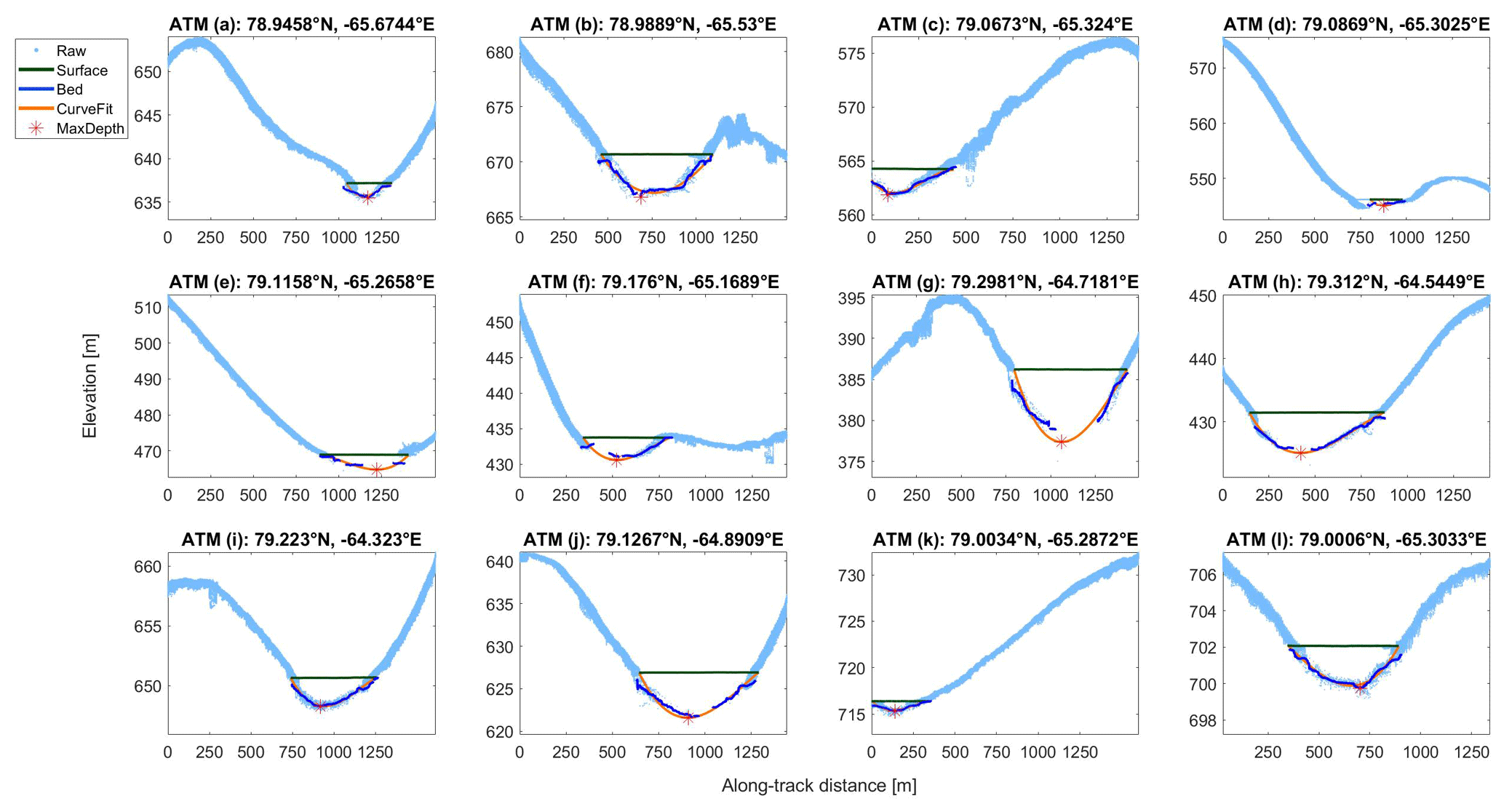
Figure 3ATM lake profiles from 17 July 2017 fitted using lake surface–bed separation, including the raw ILATM1B product, the lake surface signal, the lake bottom signal, the polynomial- and spline-fitted bottom, and the point of maximum depth. Along-track distance is relative to the start of a data granule.
Table 1Cumulative statistics for ATM supraglacial lakes explored in this study, including mean and maximum signal-based depth (ds) and polynomial-based depth (dp), along-track extent L, mean lake depth uncertainty (), and mean polynomial estimation error (). Units are in meters.
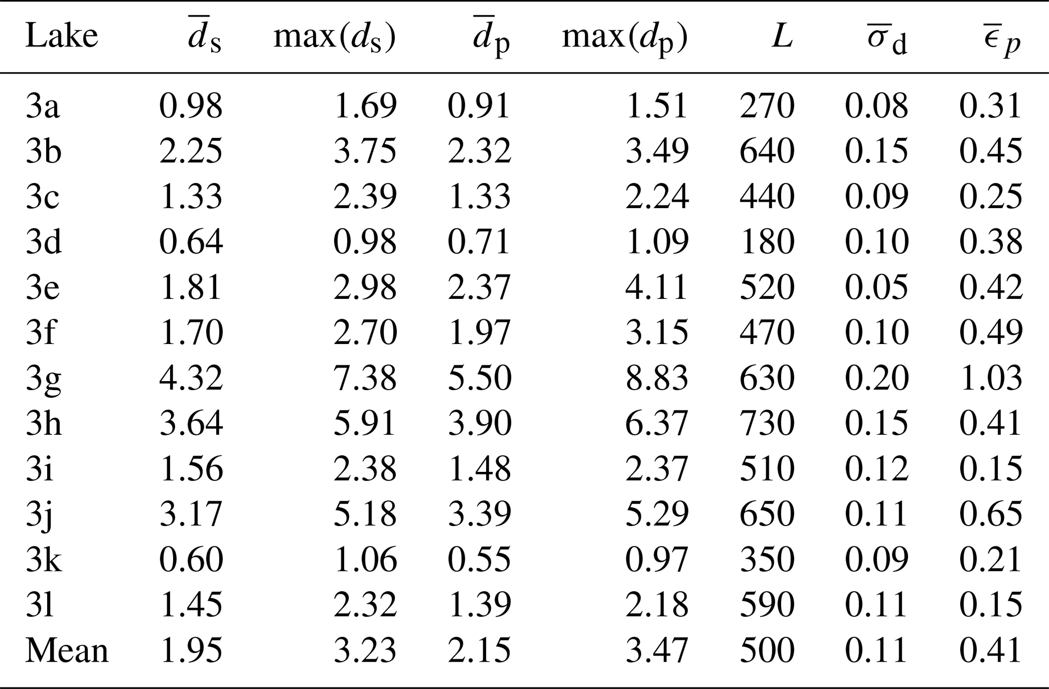
The spread in ATM lake bed photons is low (Table 1, column 7), with a maximum of 0.2 m for lake 3g. The highest uncertainties are observed for lake depths greater than 3 m, perhaps influenced by low signal-to-noise ratios or the conical scanning of the OIB lidar instrument. Polynomial estimation errors are 0.41 m on average. Several depth errors are below this mean, but a strong standard error (1.03 m) in lake 3g, due to difficulties in capturing its steep bed slope, slightly skews the mean error. Excluding this value, the mean error among ATM polynomial estimates reduces to 0.35 m.
We examined an additional 12 supraglacial lakes with ICESat-2, eight in Greenland and four on the Amery Ice Shelf in Antarctica. Three of the Antarctic melt lakes (4a, 4b, 4d) are highlighted in Magruder et al. (2019) and Fricker et al. (2020). The refined algorithm captures lake surfaces and beds reasonably well (Fig. 4), with a mean uncertainty of 0.015 m for surface photons and 0.38 m for bed photons. The lake edges partially account for the bed photon uncertainty, for the limited number of acceptable photons produces a slight bias in bed estimates. Antarctic melt lakes were generally shallower than those seen in Greenland (Table 2) – only lake 4a exceeded 3 m in depth, whereas the mean maximum depth over Greenland was 4.08 m. Melt lakes on the Amery Ice Shelf were 3–8 km in extent, thus facilitating detection in histograms. Greenland lakes exhibited a wider range of sizes, but the algorithm successfully performed retrievals for lakes as small as 200 m in extent.
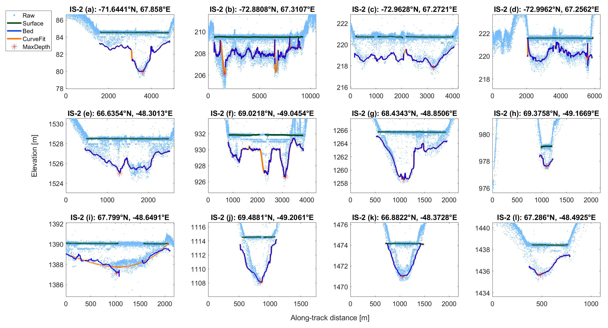
Figure 4Supraglacial lakes and melt ponds detected by ICESat-2 over the Amery Ice Shelf (a–d) and western Greenland (e–l), using Tracks 0081 and 1222, respectively.
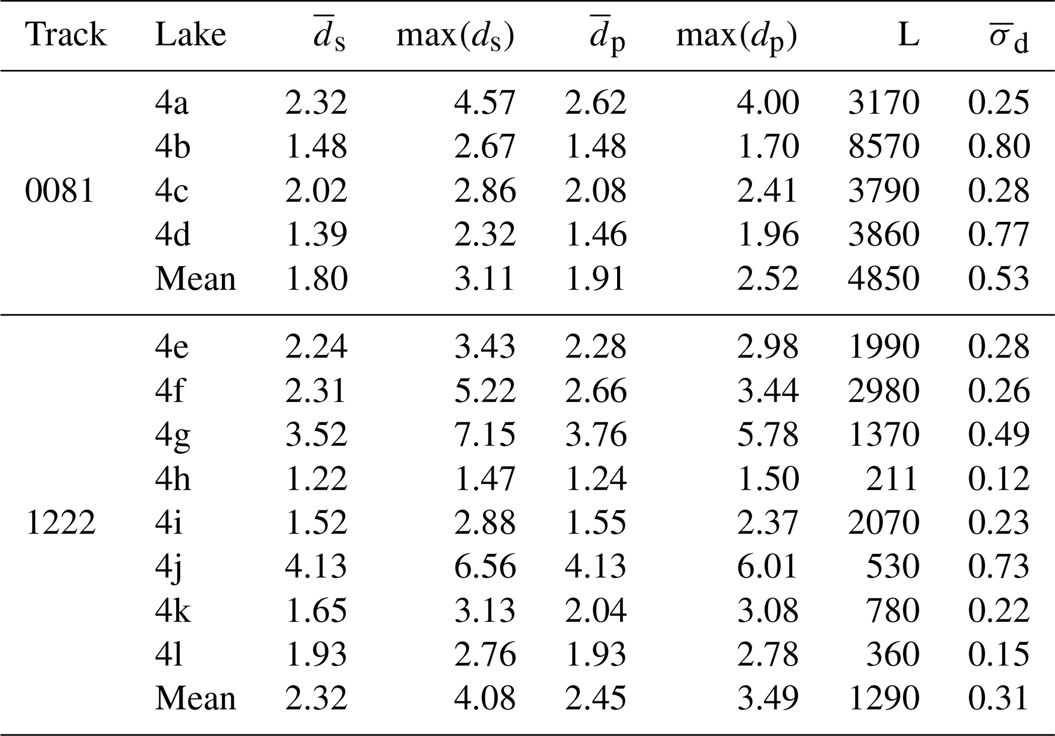
On average, the noisier data from ICESat-2 produce uncertainties greater than 0.2 m for the Antarctic lakes and 0.3 m for the Greenland lakes, as seen in Table 2, column 8. The inclusion of lower-confidence photons increases uncertainty despite the restricted bed photon criteria, for the larger photon cloud increases the spread of the entire lake profile. The curve fits improved depth estimates for lakes 4b, 4f, and 4i. Of these lakes, only 4i used a polynomial estimate due to poor spline fitting. The inclusion of interpolants increased the mean depth estimates of 4b, 4f, and 4i by 0.08 m, 0.04 m, and 0.03 m, respectively. The spline fitting significantly increased the maximum observed depth in lake 4b from 2.67 m to 3.27 m. The remaining lakes featured more complete bed profiles, meaning that the fitting estimates were less important.
5.1 Algorithm performance
The conical scanning of the ATM lidar produced oscillations in 1D elevation profiles that dampened over lake surfaces, so lakes generally were easier to identify with the airborne retrievals. Flights conducted during the OIB campaign actively avoided cloudy conditions, reducing attenuation sources and further simplifying the lake-finding process over common melt regions. The data volume per granule was lower than ATL03, resulting in less time needed to run the algorithm. However, the number of retrievals possible with ATM is limited, so observations with the lidar best serve as a validation and correction tool for ICESat-2 and other retrieval methods.
The laser power and detector sensitivity of the ATLAS instrument on board ICESat-2 are sufficient to reliably detect lake beds, and a high along-track resolution will correspond to improved estimates of lake bed topography, water depth, and water volume. Despite strong advantages, significant difficulties must be considered before automatic lake detection is feasible. At its operational altitude, the ATLAS laser is subject to first-photon bias, solar background radiation, and scattering and absorption by blowing snow and clouds. Clouds are common over the fringes of Antarctica and Greenland (Bennartz et al., 2013; Lachlan-Cope, 2010; Van Tricht et al., 2016), and often their optical depth is sufficient to render the surface undetectable. Handling the large data volumes in ATL03 granules also presents a significant challenge. A single granule provides coverage over hundreds of kilometers, so the running time of the algorithm increases relative to ATM granules. Lakes smaller than 1 km are difficult to automatically detect with the algorithm, but LSBS may still be performed for lakes as small as 200 m if the location of a lake is known through other means (e.g., Landsat-8 imagery or ATM retrievals).
We observed differences in lake topography for ICESat-2 lakes, and we attribute them to the underlying ice surfaces. Supraglacial lakes in Greenland typically form into smooth basins within depressions formed by the underlying bedrock, and their location is independent of ice motion (Echelmeyer et al., 1991). In contrast, meltwater on the Amery Ice Shelf originates from the blue ice zone, propagating along the ice surface in streams. The location of lakes and ice topography is thus tied to the flow lines of the ice shelf surface. These features are flooded in the Antarctic melt season, producing melt lakes and streams up to 80 km in length (Mellor and McKinnon, 1960; Phillips, 1998; Kingslake et al., 2017).
A potential issue for lake depth retrievals concerns specular reflection. When photons interact with a flat water surface, they may reflect directly back to the detector with minimal energy loss. The excessive return energy produces a “dead time” in the ATLAS detector, and the return signal is represented by multiple subsurface returns below the actual surface (Neumann et al., 2020). An example of this phenomenon may be seen in Fig. 4f, where a prominent subsurface return 1 m below the true surface is featured along the lake extent. However, because the subsurface echo is smaller than the true surface when viewed through histograms, the LSBS algorithm is able to avoid biases caused by specular reflection.
The success of this method for lake depth retrievals is governed by spatial and temporal sampling of the instruments across the lakes when they are full. The methods presented here are most effective when the altimeter passes directly over the deep part of a lake rather than at its edge. This provides a lake depth profile that is more representative of the complete lake, allowing for improved estimates of lake depth and extent. A complete lake profile also provides sufficient information to the LSBS algorithm, reducing the risk of false negatives that occur with small lakes or incomplete profiles. The temporal sampling of ICESat-2 and ATM is infrequent (every 91 d for ICESat-2 and random for ATM), and so the same lakes will not always be present every time these data are required. Therefore, coincident satellite imagery is desirable to simplify the lake-finding process.
5.2 Automation challenges
The identification of lake beds in the LSBS algorithm is based on a window of acceptable photons. The photon window is constrained by the coefficients a and b (for ICESat-2, a=1.0, b=0.5). Lake beds detected in this manner had a height uncertainty of 0.38 m (Table 2). The coefficients for ATM (a=1.8, b=0.75) resulted in more accurate retrievals on an individual basis. However, implementing varying a and b values proved difficult to automate, as other values may produce more accurate depths. The challenges in full automation are related to three key issues. First, the observed extent of lakes varied considerably, especially over Greenland. The diversity in lake sizes complicated attempts to derive a universal flatness check. Smaller lakes present fewer lake surface photons, so a smaller data window (∼ 104 photons) is required to prevent false positives. However, larger lakes may not be fully represented in smaller windows. A larger data window (∼ 105 photons) will fully capture the largest lakes, but smaller lakes may then be overlooked.
Second, multiple scattering at the lake bed increases the photon spread and thus also increases the uncertainty of depth retrievals. Most supraglacial lakes observed by ATM featured smooth beds, so photons experienced one or few scattering events before returning to the detector. The instrument digitizer automatically filters return signals with low photon counts, reducing the spread of bed photons, at the cost of deep lake bottom detection. In contrast, the lakes observed with ICESat-2 exhibited more heterogeneous beds, leading to increased scattering events by photons and delays in return pulses. In these cases, the given values for a and b may not produce the most accurate bed solution. Furthermore, if the return is significant for a given photon window, then it may lead to a false negative for a portion of the lake (Fig. 4i). To reduce uncertainty in lake depth retrievals, future improvements in working with ICESat-2 data should focus on identifying and filtering multiple scattering.
Finally, the ATL03 signal-finding algorithm is conservative in that it accepts false positives (background photons classified as signal photons) to ensure that all signal photons are passed to higher-level products. Thus, uncertainties in the ATL03 photon classification contribute to noise in the water column and the lake bed. The classification algorithm uses predefined surface masks to allocate statistical confidence to ATL03 photons for multiple surface types (e.g. inland water, land ice, land), with overlap possible between masks (Neumann et al., 2020). Melt lakes are categorized as land ice (lake surface) and land (lake surface and bed). Because the land classification also includes the bed, it includes more potential signal photons than land ice, so our recommendation is to only use land photons for supraglacial lake depth retrievals. It must be noted, however, that a lake bed profile is fully resolved only with the inclusion of low- and medium-confidence and buffer photons. The buffer photons ensure that all photons identified as surface signal are provided to the appropriate upper-level data product algorithms. However, they can introduce greater noise to the profile, so more sophisticated filtering techniques are needed to distinguish between signal photons and the solar background.
We present a method to detect supraglacial lakes and estimate lake depth from 532 nm laser altimetry data. We establish test cases for lake detection over two regions of Greenland (Hiawatha Glacier, 19 July 2017 and Jakobshavn Isbræ, 17 June 2019) and East Antarctica (Amery Ice Shelf, 2 January 2019), and our results demonstrate that depth retrievals are possible using laser altimetry. Verification of lake detection is given with lake surface flatness tests, where we observe low topographical variance over lake surfaces relative to surrounding ice. Lake bottoms are easy to identify once lake surfaces are established, given that the lakes are not deeper than 7 m.
We introduce a lake surface–bed separation scheme for ATM and ICESat-2 geolocated photon data to determine the maximum depth of lakes. Our results indicate that altimetry signals reliably detect bottoms as deep as 7 m, after which absorption of the photons in water reduces the number of reflected photons. Heterogeneity at the lake bed also produces attenuation, complicating retrieval attempts for lakes with rough bed topography or with high impurity concentration. Additional work is required to assess the impacts of lake impurities and geometry on altimetry signals and to improve estimates for such cases. Despite these shortcomings, we anticipate retrieval capability to improve as observations from the 2019 and 2020 Arctic melt seasons are released.
We establish the feasibility for estimates of supraglacial lake depth over Antarctica and Greenland. The high accuracy of 532 nm laser altimeters allows these results to serve as a benchmark for future retrieval studies. Future studies need to examine the accuracy of ICESat-2 lake retrievals relative to ATM where applicable, with additional comparisons to depth estimates from passive imaging sensors.
ICESat-2 ATL03 V002 and ATM L1B V002 data may be accessed from https://doi.org/10.5067/ATLAS/ATL03.002 (Neumann et al., 2019a) and https://doi.org/10.5067/19SIM5TXKPGT (Studinger, 2013), respectively. Depth data for lakes in Fig. 3 are available upon request from Zachary Fair. Depth data for the supraglacial lakes given in Fig. 4 are available at https://doi.org/10.5281/zenodo.3838274 (Fair, 2020). The LSBS algorithm and its subroutines may also be accessed from https://doi.org/10.5281/zenodo.3838274 (Fair, 2020).
The authors declare that they have no conflict of interest.
We would like to thank Allen Pope and the anonymous reviewer for their constructive comments that improved the quality of the paper. We are also grateful for the ICESat-2 and Operation IceBridge teams for their insight into the two lidars.
This research was supported by the NASA Earth and Space Science Fellowship (grant no. 19-EARTH19R-0047) and NASA grant 80NSSC20K0062.
This paper was edited by Louise Sandberg Sørensen and reviewed by Allen Pope and one anonymous referee.
Abdalati, W., Zwally, H. J., Bindschadler, R., Csatho, B., Farrell, S. L., Fricker, H. A., Harding, D., Kwok, R., Lefsky, M., Markus, T., Marshak, A., Neumann, T., Palm, S., Schutz, B., Smith, B., Spinhirne, J., and Webb, C.: The ICESat-2 Laser Altimetry Mission, P. IEEE, 98, 735–751, https://doi.org/10.1109/JPROC.2009.2034765, 2010. a
Banwell, A. F., Arnold, N. S., Willis, I. C., Tedesco, M., and Ahlstrøm, A. P.: Modeling supraglacial water routing and lake filling on the Greenland Ice Sheet, J. Geophys. Res.-Earth, 117, F04012, https://doi.org/10.1029/2012JF002393, 2012. a
Banwell, A. F., MacAyeal, D. R., and Sergienko, O. V.: Breakup of the Larsen B Ice Shelf triggered by chain reaction drainage of supraglacial lakes, Geophys. Res. Lett., 40, 5872–5876, https://doi.org/10.1002/2013GL057694, 2013. a
Bennartz, R., Shupe, M. D., Turner, D. D., Walden, V. P., Steffen, K., Cox, C. J., Kulie, M. S., Miller, N. B., and Petterson, C.: July 2012 Greenland melt extent enhanced by low-level liquid clouds, Nature, 496, 83–86, https://doi.org/10.1038/nature12002, 2013. a
Box, J. E. and Ski, K.: Remote sounding of Greenland supraglacial melt lakes: implications for subglacial hydraulics, J. Glaciol., 53, 257–265, https://doi.org/10.3189/172756507782202883, 2007. a
Brock, J. C., Wright, C. W., Sallenger, A. H., Krabill, W., and Swift, R.: Basis and Methods of NASA Airborne Topographic Mapper Lidar Surveys for Coastal Studies, J. Coastal Res., 18, 1–13, 2002. a, b
Brunt, K. M., Neumann, T. A., Amundson, J. M., Kavanaugh, J. L., Moussavi, M. S., Walsh, K. M., Cook, W. B., and Markus, T.: MABEL photon-counting laser altimetry data in Alaska for ICESat-2 simulations and development, The Cryosphere, 10, 1707–1719, https://doi.org/10.5194/tc-10-1707-2016, 2016. a
Brunt, K. M., Neumann, T. A., and Larsen, C. F.: Assessment of altimetry using ground-based GPS data from the 88S Traverse, Antarctica, in support of ICESat-2, The Cryosphere, 13, 579–590, https://doi.org/10.5194/tc-13-579-2019, 2019a. a
Brunt, K. M., Neumann, T. A., and Smith, B. E.: Assessment of ICESat-2 Ice Sheet Surface Heights, Based on Comparisons Over the Interior of the Antarctic Ice Sheet, Geophys. Res. Lett., 46, 13072–13078, https://doi.org/10.1029/2019GL084886, 2019b. a, b
Catania, G. A., Neumann, T. A., and Price, S. F.: Characterizing englacial drainage in the ablation zone of the Greenland ice sheet, J. Glaciol., 54, 567–578, https://doi.org/10.3189/002214308786570854, 2008. a
Chen, X., Huang, X., and Flanner, M. G.: Sensitivity of modeled far-IR radiation budgets in polar continents to treatments of snow surface and ice cloud radiative properties, Geophys. Res. Lett., 41, 6530–6537, https://doi.org/10.1002/2014GL061216, 2014. a
Curry, J. A., Rossow, W. B., Randall, D., and Schramm, J. L.: Overview of Arctic Cloud and Radiation Characteristics, J. Climate, 9, 1731–1764, 1996. a
Das, S. B., Joughin, I., Behn, M. D., Howat, I. M., King, M. A., Lizarralde, D., and Bhatia, M. P.: Fracture Propagation to the Base of the Greenland Ice Sheet During Supraglacial Lake Drainage, Science, 320, 778–781, https://doi.org/10.1126/science.1153360, 2008. a
Echelmeyer, K., Clarke, T. S., and Harrison, W. D.: Surficial glaciology of Jakobshavns Isbrae, West Greenland: Part I. Surface morphology, J. Glaciol., 37, 368–382, 1991. a, b
Fair, Z.: ICESat-2 Supraglacial Lake Depth Data, Zenodo, https://doi.org/10.5281/zenodo.3838274, 2020. a, b
Fitzpatrick, A. A. W., Hubbard, A. L., Box, J. E., Quincey, D. J., van As, D., Mikkelsen, A. P. B., Doyle, S. H., Dow, C. F., Hasholt, B., and Jones, G. A.: A decade (2002–2012) of supraglacial lake volume estimates across Russell Glacier, West Greenland, The Cryosphere, 8, 107–121, https://doi.org/10.5194/tc-8-107-2014, 2014. a
Fricker, H. A., Arndt, P., Adusumilli, S., Brunt, K. M., Datta, T., Fair, Z., Jasinski, M., Kingslake, J., Magruder, L., Moussavi, M., Pope, A., and Spergel, J. J.: ICESat-2 meltwater depth retrievals: application to surface melt on southern Amery Ice Shelf, East Antarctica, Geophys. Res. Lett., in press, 2020. a
Georgiou, S., Shepherd, A., McMillan, M., and Nienow, P.: Seasonal evolution of supraglacial lake volume from ASTER imagery, Ann. Glaciol., 50, 95–100, https://doi.org/10.3189/172756409789624328, 2009. a
Howat, I. M., de la Peña, S., van Angelen, J. H., Lenaerts, J. T. M., and van den Broeke, M. R.: Brief Communication “Expansion of meltwater lakes on the Greenland Ice Sheet”, The Cryosphere, 7, 201–204, https://doi.org/10.5194/tc-7-201-2013, 2013. a
Huang, X., Chen, X., Flanner, M., Yang, P., Feldman, D., and Kuo, C.: Improved Representation of Surface Spectral Emissivity in a Global Climate Model and Its Impact on Simulated Climate, J. Climate, 31, 3711–3727, https://doi.org/10.1175/JCLI-D-17-0125.1, 2018. a
Humphrey, N. F., Harper, J. T., and Pfeffer, W. T.: Thermal tracking of meltwater retention in Greenland's accumulation area, J. Geophys. Res.-Earth, 117, F01010, https://doi.org/10.1029/2011JF002083, 2012. a
Jasinski, M. F., Stoll, J. D., Cook, W. B., Ondrusek, M., Stengel, E., and Brunt, K.: Inland and near-shore water profiles derived from the high-altitude Multiple Altimeter Beam Experimental Lidar (MABEL), J. Coast. Res., 76, 44–55, 2016. a
Kingslake, J., Ely, J. C., Das, I., and Bell, R. E.: Widespread movement of meltwater onto and across Antarctic ice shelves, Nature, 544, 349–352, https://doi.org/10.1038/nature22049, 2017. a
Krabill, W., Abdalati, W., Frederick, E., Manizade, S., Martin, C., Sonntag, J., Swift, R., Thomas, R., and Yungel, J.: Aircraft laser altimetry measurement of elevation changes of the greenland ice sheet: technique and accuracy assessment, J. Geodynam., 34, 357–376, https://doi.org/10.1016/S0264-3707(02)00040-6, 2002. a
Lachlan-Cope, T.: Antarctic clouds, Polar Res., 29, 150–158, https://doi.org/10.3402/polar.v29i2.6065, 2010. a
Leeson, A. A., Shepherd, A., Briggs, K., Howat, I., Fettweis, X., Morlighem, M., and Rignot, E.: Supraglacial lakes on the Greenland ice sheet advance inland under warming climate, Nat. Clim. Change, 5, 51–55, https://doi.org/10.1038/nclimate2463, 2015. a
Liang, Y.-L., Colgan, W., Lv, Q., Steffen, K., Abdalati, W., Stroeve, J., Gallaher, D., and Bayou, N.: A decadal investigation of supraglacial lakes in West Greenland using a fully automatic detection and tracking algorithm, Remote Sens. Environ., 123, 127–138, https://doi.org/10.1016/j.rse.2012.03.020, 2012. a
Lüthje, M., Pedersen, L., Reeh, N., and Greuell, W.: Modelling the evolution of supraglacial lakes on the West Greenland ice-sheet margin, J. Glaciol., 52, 608–618, https://doi.org/10.3189/172756506781828386, 2006. a
Ma, Y., Xu, N., Sun, J., Wang, X. H., Yang, F., and Li, S.: Estimating water levels and volumes of lakes dated back to the 1980s using Landsat imagery and photon-counting lidar datasets, Remote Sens. Environ., 232, 111287, https://doi.org/10.1016/j.rse.2019.111287, 2019. a
Magruder, M., Fricker, H. A., Farrell, S. L., Brunt, K. M., Gardner, A., Hancock, D., Harbeck, K., Jasinkski, M., Kwok, R., Kurtz, N., Lee, J., Markus, T., Morison, J., Neuenschwander, A., Palm, S., Popescu, S., Smith, B., and Yang, Y.: New Earth orbiter provides a sharper look at a changing planet, Eos, 100, https://doi.org/10.1029/2019EO133233, 2019. a
Markus, T., Neumann, T., Martino, A., Abdalati, W., Brunt, K., Csatho, B., Farrell, S., Fricker, H., Gardner, A., Harding, D., Jasinski, M., Kwok, R., Magruder, L., Lubin, D., Luthcke, S., Morison, J., Nelson, R., Neuenschwander, A., Palm, S., Popescu, S., Shum, C., Schutz, B. E., Smith, B., Yang, Y., and Zwally, J.: The Ice, Cloud, and land Elevation Satellite-2 (ICESat-2): Science requirements, concept, and implementation, Remote Sens. Environ., 190, 260–273, https://doi.org/10.1016/j.rse.2016.12.029, 2017. a
Martin, C. F., Krabill, W. B., Manizade, S. S., Russel, R. L., Sonntag, J. G., Swift, R. N., and Yungel, J. K.: Airborne Topographic Mapper Calibration Procedures and Accuracy Assessment, Tech. Rep. 215891, NASA Goddard Space Flight Center, available at: https://ntrs.nasa.gov/archive/nasa/casi.ntrs.nasa.gov/20120008479.pdf (last access: 5 August 2019), 2012. a
McMillan, M., Nienow, P., Shepherd, A., Benham, T., and Sole, A.: Seasonal evolution of supra-glacial lakes on the Greenland Ice Sheet, Earth Planet. Sc. Lett., 262, 484–492, https://doi.org/10.1016/j.epsl.2007.08.002, 2007. a
Mellor, M. and McKinnon, G.: The Amery Ice Shelf and its hinterland, Polar Rec., 10, 30–34, https://doi.org/10.1017/S0032247400050579, 1960. a
Morassutti, M. P. and Ledrew, E. F.: Albedo and depth of melt ponds on sea-ice, Int. J. Climatol., 16, 817–838, https://doi.org/10.1002/(SICI)1097-0088(199607), 1996. a
Mouginot, J., Rignot, E., Bjørk, A., van den Broeke, M., Millan, R., Morlighem, M., Noël, B., Scheuchl, B., and Wood, M.: Forty-six years of Greenland Ice Sheet mass balance from 1972 to 2018, P. Natl. Acad. Sci. USA, 116, 9239–9244, https://doi.org/10.1073/pnas.1904242116, 2019. a
Moussavi, M. S., Abdalati, W., Pope, A., Scambos, T., Tedesco, M., MacFerrin, M., and Grigsby, S.: Derivation and validation of supraglacial lake volumes on the Greenland Ice Sheet from high-resolution satellite imagery, Remote Sens. Environ., 183, 294–303, https://doi.org/10.1016/j.rse.2016.05.024, 2016. a
Moussavi, M., Pope, A., Halberstadt, A. R. W., Trusel, L. D., Cioffi, L., and Abdalati, W.: Antarctic Supraglacial Lake Detection Using Landsat 8 and Sentinel-2 Imagery: Towards Continental Generation of Lake Volumes, Remote Sens., 12, 134, https://doi.org/10.3390/rs12010134, 2020. a
Neumann, T. A., Brenner, A., Hancock, D., Robbins, J., Luthcke, S. B., Harbeck, K., Lee, J., Gibbons, A., Saba, J., and Brunt, K.: ATLAS/ICESat-2 L2A Global Geolocated Photon Data, Version 2, https://doi.org/10.5067/ATLAS/ATL03.001 2019a. a, b
Neumann, T. A., Martino, A. J., Markus, T., Bae, S., Bock, M. R., Brenner, A. C., Brunt, K. M., Cavanaugh, J., Fernandes, S. T., Hancock, D. W., Harbeck, K., Lee, J., Kurtz, N. T., Luers, P. J., Luthcke, S. B., Margruder, L., Penningtin, T. A., Ramos-Izquierdo, L., Rebold, T., Skoog, J., and Thomas, T. C.: The Ice, Clouds and Land Elevation Satellite-2 mission: A global geolocated photon product derived from the Advanced Topographic Laser Altimeter System, Remote Sens. Environ., 233, 111325, https://doi.org/10.1016/j.rse.2019.111325, 2019b. a, b, c
Neumann, T., Brenner, A., Hancock, D., Robbins, J., Saba, J., Harbeck, K., Gibbons, A., Lee, J., Luthcke, S., and Rebold, T.: Ice, Clouds, and Land Elevation Satellite-2 (ICESat-2): Algorithm Theoretical Basis Document (ATBD) for Geolocated Photons, Tech. rep., NASA Goddard Space Flight Center, available at: https://icesat-2.gsfc.nasa.gov/sites/default/files/u71/ICESat2_ATL03_ATBD_r003_v2.pdf, last access: 8 June 2020. a, b
Parizek, B. R. and Alley, R. B.: Implications of increased Greenland surface melt under global-warming scenarios: ice-sheet simulations, Quaternary Sci. Rev., 23, 1013–1027, 2004. a
Parrish, C. E., Magruder, L. A., Neuenschwander, A. L., Forfinski-Sarkozi, N., Alonzo, M., and Jasinki, M.: Validation of ICESat-2 ATLAS bathymetry and analysis of ATLAS's bathymetric mapping performance, Remote Sens., 11, 1634, https://doi.org/10.3390/rs11141634, 2019. a, b
Phillips, H. A.: Surface meltstreams on the Amery Ice Shelf, East Antarctica, Ann. Glaciol., 27, 177–181, 1998. a
Philpot, W. D.: Bathymetric mapping with passive multispectral imagery, Appl. Optics, 28, 1569–1578, https://doi.org/10.1364/AO.28.001569, 1989. a
Pope, A.: Reproducibly estimating and evaluating supraglacial lake depth with Landsat 8 and other multispectral sensors, Earth and Space Science, 3, 176–188, https://doi.org/10.1002/2015EA000125, 2016. a
Pope, A., Scambos, T. A., Moussavi, M., Tedesco, M., Willis, M., Shean, D., and Grigsby, S.: Estimating supraglacial lake depth in West Greenland using Landsat 8 and comparison with other multispectral methods, The Cryosphere, 10, 15–27, https://doi.org/10.5194/tc-10-15-2016, 2016. a
Rignot, E., Mouginot, J., Scheuchl, B., van den Broeke, M., van Wessem, M. J., and Morlighem, M.: Four decades of Antarctic Ice Sheet mass balance from 1979–2017, P. Natl. Acad. Sci. USA, 116, 1095–1103, https://doi.org/10.1073/pnas.1812883116, 2019. a
Selmes, N., Murray, T., and James, T. D.: Fast draining lakes on the Greenland Ice Sheet, Geophys. Res. Lett., 38, L15501, https://doi.org/10.1029/2011GL047872, 2011. a
Smith, B., Fricker, H., Holschuh, N., Gardner, A. S., Adusumilli, S., Brunt, K. M., Csatho, B., Harbeck, K., Huth, A., Neumann, T., Nilsson, J., and Siegfried, M.: Land ice height-retrieval algorithm for NASA's ICESat-2 photon-counting laser altimeter, Remote Sens. Environ., 233, 111352, https://doi.org/10.1016/j.rse.2019.111352, 2019. a, b
Sneed, W. A. and Hamilton, G. S.: Evolution of melt pond volume on the surface of the Greenland Ice Sheet, Geophys. Res. Lett., 34, L03501, https://doi.org/10.1029/2006GL028697, 2007. a
Studinger, M.: IceBridge ATM L1B Elevation and Return Strength, Version 2, https://doi.org/10.5067/19SIM5TXKPGT, 2013 (updated 2018). a, b
Stumpf, R. P., Holderied, K., and Sinclair, M.: Determination of water depth with high-resolution satellite imagery over variable bottom types, Limnol. Oceanogr., 48, 547–556, https://doi.org/10.4319/lo.2003.48.1_part_2.0547, 2003. a
Tedesco, M. and Steiner, N.: In-situ multispectral and bathymetric measurements over a supraglacial lake in western Greenland using a remotely controlled watercraft, The Cryosphere, 5, 445–452, https://doi.org/10.5194/tc-5-445-2011, 2011. a
van den Broeke, M. R., Enderlin, E. M., Howat, I. M., Kuipers Munneke, P., Noël, B. P. Y., van de Berg, W. J., van Meijgaard, E., and Wouters, B.: On the recent contribution of the Greenland ice sheet to sea level change, The Cryosphere, 10, 1933–1946, https://doi.org/10.5194/tc-10-1933-2016, 2016. a
Van Tricht, K., Lhermitte, S., Lenaerts, J. T. M., Gorodetskaya, I. V., L'Ecuyer, T. S., Noël, B., van den Broeke, M. R., Turner, D. D., and van Lipzig, N. P. M.: Clouds enhance Greenland ice sheet meltwater runoff, Nat. Commun., 7, 10266, https://doi.org/10.1038/ncomms10266, 2016. a
Vaughan, D., Comiso, J., Allison, I., Carrasco, J., Kaser, G., Kwok, R., Mote, P., Murray, T., Paul, F., Ren, J., Rignot, E., Solomina, O., Steffen, K., and Zhang, T.: Chapter 4: Observations: Cryosphere, Tech. rep., IPCC AR5 WG1, 2013. a
Williamson, A. G., Arnold, N. S., Banwell, A. F., and Willis, I. C.: A Fully Automated Supraglacial lake area and volume Tracking (“FAST”) algorithm: Development and application using MODIS imagery of West Greenland, Remote Sens. Environ., 196, 113–133, https://doi.org/10.1016/j.rse.2017.04.032, 2017. a
Zwally, H. J., Abdalati, W., Herring, T., Larson, K., Saba, J., and Steffen, K.: Surface Melt-Induced Acceleration of Greenland Ice-Sheet Flow, Science, 297, 218–222, https://doi.org/10.1126/science.1072708, 2002. a