the Creative Commons Attribution 4.0 License.
the Creative Commons Attribution 4.0 License.
 | 24 Nov 2020
The influence of föhn winds on annual and seasonal surface melt on the Larsen C Ice Shelf, Antarctica
Amélie Kirchgaessner
Andrew N. Ross
John C. King
Peter Kuipers Munneke
Warm, dry föhn winds are observed over the Larsen C Ice Shelf year-round and are thought to contribute to the continuing weakening and collapse of ice shelves on the eastern Antarctic Peninsula (AP). We use a surface energy balance (SEB) model, driven by observations from two locations on the Larsen C Ice Shelf and one on the remnants of Larsen B, in combination with output from the Antarctic Mesoscale Prediction System (AMPS), to investigate the year-round impact of föhn winds on the SEB and melt from 2009 to 2012. Föhn winds have an impact on the individual components of the surface energy balance in all seasons and lead to an increase in surface melt in spring, summer and autumn up to 100 km away from the foot of the AP. When föhn winds occur in spring they increase surface melt, extend the melt season and increase the number of melt days within a year. Whilst AMPS is able to simulate the percentage of melt days associated with föhn with high skill, it overestimates the total amount of melting during föhn events and non-föhn events. This study extends previous attempts to quantify the impact of föhn on the Larsen C Ice Shelf by including a 4-year study period and a wider area of interest and provides evidence for föhn-related melting on both the Larsen C and Larsen B ice shelves.
- Article
(9101 KB) - Full-text XML
- BibTeX
- EndNote


In July 2017, an iceberg of approximately 6000 km2 calved off the Larsen C Ice Shelf (Hogg and Gudmundsson, 2017), located on the eastern side of the Antarctic Peninsula (AP). Some decades earlier, in 1997 and 2002, the more northerly Larsen A and B ice shelves collapsed almost entirely. This rapid disintegration had been preceded by a series of iceberg calving events in previous years, which caused the calving front to recede beyond a compressive arch that provided stability to the ice shelves (Doake et al., 1998). Since the collapse of Larsen A and B, the rate of discharge of glaciers previously feeding these ice shelves has increased, contributing to loss of land ice (Rignot et al., 2004). Therefore, increased attention is now given to observing the response of the Larsen C Ice Shelf to the 2017 calving event and to anticipating its likely response to future calving events.
The collapse of Larsen A and B was facilitated by a process known as hydrofracture, whereby ice is weakened due to drainage of surface meltwater into crevasses and increased pressure from ponds of standing meltwater forming on the ice shelf surface (Scambos, 2004; Robel and Banwell, 2019). Recently, Robel and Banwell (2019) confirmed that the rapid rate of collapse of Larsen B (only a few weeks) was caused by an anomalously large, sudden and widespread surface melt event, which triggered successive or simultaneous hydrofracturing. Surface melt has increased strongly in this region since the middle of the 20th century (Cape et al., 2015). As on Larsen A and B (Scambos et al., 2000), surface ponding is a common feature on the northwest portion of Larsen C (Luckman et al., 2014) but not elsewhere on the shelf in the current climate. However, surface melt is projected to increase strongly on Larsen C in the coming century (Trusel et al., 2015; Bell et al., 2018). For that reason, it is important to understand the conditions that lead to surface melt and its future impact on ice shelf stability.
On the ice shelves east of the AP, surface melt is partially caused by föhn winds. These relatively warm and dry winds are caused by westerly airflow over the AP mountain range. Under the right conditions, föhn winds enhance surface melt by providing heat and increased solar radiation to the surface (King et al., 2017). Marshall et al. (2006) proposed that a trend towards an increasingly positive Southern Annular Mode (SAM) index in the late 1960s led to a strengthening and southward movement of the circumpolar westerly winds. This increased the flow of air over the AP and consequently led to an increase in the number of föhn events on the eastern side of the AP, leading to increased surface melt. Indeed, a recent study by Cape et al. (2015) identified a positive correlation between the SAM and the frequency with which föhn winds were observed over the northern AP for 2 decades, 1962–1972 and 1999–2010.
Several studies have investigated the origin and characteristics of föhn winds over the Larsen C Ice Shelf (King et al., 2008; Grosvenor et al., 2014; Elvidge et al., 2015; Turton et al., 2018; Wiesenekker et al., 2018; Kirchgaessner et al., 2019). Föhn jets are often present during westerly flows, where the föhn air descends through gaps in the topography as well as over the main ridge of the mountains (Elvidge et al., 2015). Depending on whether the westerly flow is linear or non-linear (Elvidge et al., 2016), the effect of föhn can be localised but intense (non-linear flow) or extensive but weaker (linear flow). The influence of föhn winds is observable over 100 km from the foot of the AP (Kuipers Munneke et al., 2012; Turton et al., 2018). Föhn winds occur year-round and 15 % of the time from 2009 to 2012 (Turton et al., 2018). Wiesenekker et al. (2018) found a similar percentage of 14 % between 2014 and 2016 but also found that their occurrence is highly variable on longer timescales. Föhn wind frequency is highly variable from season to season over Larsen C: they occur most often during spring, when they can dominate the weather conditions for 65 % of the time (Turton et al., 2018).
The influence of föhn winds on the surface of the ice shelves along the AP has been a recent focus for modelling and observational studies. Luckman et al. (2014) demonstrated that the occurrence of melt ponds over Larsen C relates to the frequency of föhn winds. Similarly, Cape et al. (2015) identified strong correlations between the occurrence of föhn events and the frequency of surface melt and the near-surface air temperature in the area of Larsen A and B. Leeson et al. (2017) also suggested that surface melting of Larsen B prior to its collapse was driven by föhn winds. Most recently, Datta et al. (2019) analysed how the frequency of föhn winds influences snowmelt, density and depth of water percolation over Larsen C using a regional climate model and remote sensing data. Studies investigating how föhn winds specifically influence the surface energy budget (SEB) components, which are then responsible for melting, are less common and therefore explored here.
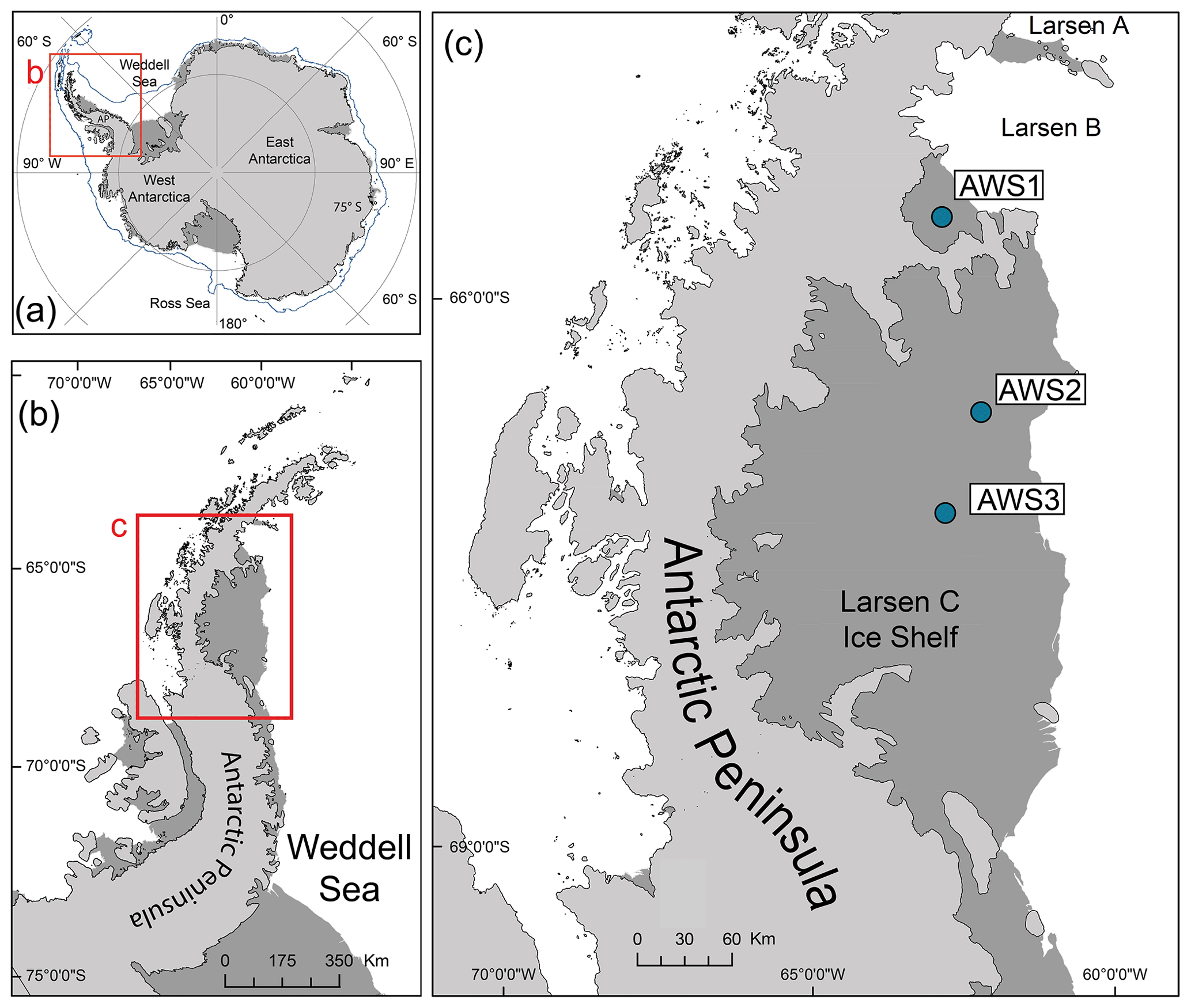
Figure 1(a) A map of the Antarctic continent, with a blue line showing the average sea ice extent and a red box outlining the area in (b). (b) A map of the Antarctic Peninsula (light grey) and ice shelves (dark grey), with a red box indicating the area shown in (c). (c) A map of the Larsen C Ice Shelf with the three AWS locations marked with blue dots. Coastlines and sea ice extent are imported from the Antarctic Digital Database. This figure is adapted from Turton et al. (2018).
In the summertime SEB, a positive net radiative flux (fluxes directed towards the surface are defined as positive) is only partly offset by negative turbulent fluxes of sensible and latent heat (Van den Broeke, 2005). The excess energy is used for heating and melting of snow. On average, the surface melt rate of the Larsen C Ice Shelf, derived from satellites and models, is approximately 250 mm w.e. yr−1 but can exceed 400 mm w.e. yr−1 in the north (Trusel et al., 2013). During winter, heat is extracted from the snow due to net longwave cooling in the absence of solar radiation. A few studies have attempted to quantify the impact of föhn winds on the SEB. For example, Kuipers Munneke et al. (2018) used observations from one location on Larsen C, at the foot of the AP mountains, to study föhn winds during winter. They identified that 23 % of the annual melt flux at this location was produced during winter (JJA) due to the occurrence of föhn winds. King et al. (2017) analysed the effect of föhn winds on the SEB during the 2010–2011 spring melt season using observations and the Antarctic Mesoscale Prediction System (AMPS). However, these studies have only focused on a number of case studies, during particular seasons with a large number of föhn winds or for a particular location on Larsen C. Understanding of the interannual and seasonal influence of föhn winds on the SEB and melt characteristics is currently lacking, and therefore all seasons are investigated in this study. Our current understanding is largely from analysing extreme melting episodes related to föhn winds (e.g. November 2010; King et al., 2017; Kuipers Munneke et al., 2012). Whether föhn winds are responsible for melting under more typical conditions and, if so, which of the SEB components are influenced are not as well understood and are therefore explored in this study. Due to the break-up of Larsen B, observations on this ice shelf are limited, and previous studies investigating the role of föhn winds have focused on Larsen C. Here, we use a SEB model along with observations on the remnants of Larsen B (Scar Inlet) to understand the potential impact of föhn winds in this more northerly setting, for the first time.
In this study, we analyse the composite effects of föhn against non-föhn periods on the SEB and melt production for both the Larsen C and Larsen B (remnants) ice shelves, inter- and intra-annually. By doing so, we investigate the impact of föhn winds on each season with the hypothesis that the impact is highest in spring, when föhn winds are more frequent. Furthermore, we analyse observationally derived model output from a previously unpublished dataset (on Scar Inlet) in combination with high-resolution AMPS output from 2009 to 2012, to provide a wider spatial analysis than many previous studies.
We use three sources of data in this study: automatic-weather-station (AWS) observations, a SEB model driven by the AWS data and archived output from the Antarctic Mesoscale Prediction System (AMPS).
2.1 AWS observations
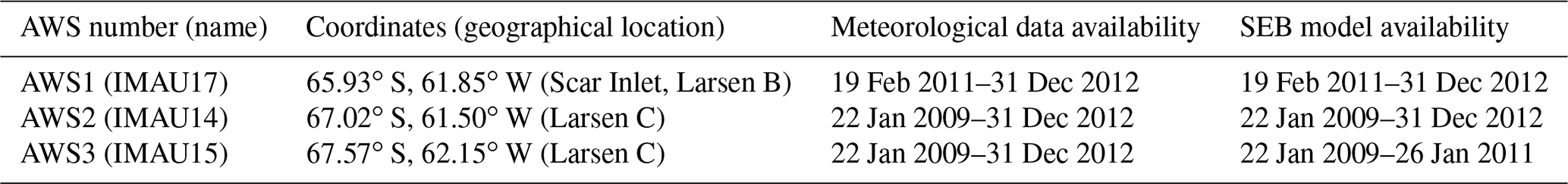
Near-surface meteorological data, radiation fluxes and subsurface temperature were observed at two locations on Larsen C (AWS2 and AWS3) and one (AWS1) on Scar Inlet, a remnant of Larsen B (Table 1 and Fig. 1). AWS2 and AWS3 are approximately 100 km away from the foot of the AP mountains. AWS1 is located further north and approximately 25 km away from the AP. Therefore, it observes warmer and more frequent föhn winds (Turton et al., 2018). All three stations were located at ∼50 m a.s.l. when initially erected. Meteorological observations spanning 22 January 2009 to 31 December 2012 (at AWS2 and AWS3) and 19 February 2011 to 31 December 2012 (AWS1) were analysed in this study (Table 1). For this latter period, there is complete coverage by AMPS, the SEB model and observations. Observations were collected every 6 min, from which hourly values were derived and stored. All AWSs are owned and operated by the Institute for Marine and Atmospheric Research Utrecht (IMAU) in the Netherlands and maintained by staff of the British Antarctic Survey. For information on instrumentation and sensors, see Kuipers Munneke et al. (2012).
Table 1The metadata for the AWS observations. In the current paper, the AWS locations are numbers, following Turton et al. (2018). We have also provided the name used in other studies in brackets.
In order to compare the relative influence of solar radiation during föhn in different seasons, and following King et al. (2017), we compute atmospheric transmissivity (τ) as
where SW↓TOP is the incident shortwave radiation at the top of the atmosphere. This allows the impact of föhn conditions on SW↓ to be assessed without seasonal bias due to the extreme changes in potentially available sunlight. SW↓TOP is an output from the SEB model of Kuipers Munneke et al. (2009) as outlined in Sect. 2.2.
2.2 SEB model
We used a previously published and validated SEB model, in conjunction with AWS data input, to compute the surface energy balance at AWS2 and AWS3 (Kuipers Munneke et al., 2009, 2012). Daily averages, derived from the SEB model's hourly output, are analysed in this study. Only a brief overview of the SEB model is provided here, but a detailed description is given in Kuipers Munneke et al. (2012). The SEB is here defined as
where SW↓ and SW↑ are the incoming and outgoing shortwave radiation respectively, LW↓ and LW↑ are the incoming and outgoing longwave radiation, Hsen is the sensible heat flux, Hlat is the latent heat flux, G is the ground heat flux, and Q is the amount of shortwave radiation absorbed by the subsurface due to the penetration of the radiation into the snowpack. E is the net energy flux, taking into account the surface and subsurface melting, that is available to heat, melt or cool the ice surface (King et al., 2017). We use the sign convention that all fluxes are positive when directed towards the surface. Therefore, a positive E means that the surface is warming and/or melting. To define periods where melt is possible, the following condition is followed:
The additional term Emelt states that melting is possible and is equal to the residual of the SEB calculation (E), when the skin temperature (TSK) is at the melting point. Otherwise, the additional energy is not used for melting.
The sensible and latent heat fluxes are calculated using the bulk flux method. The ground heat flux is calculated using a multilayer snowpack model, which allows for multiple layers of melting, percolation and refreezing of meltwater (Kuipers Munneke et al., 2012). Within the multilayer snowpack module, the vertically integrated change in heat content is calculated to compute the ground heat flux (G). The temperature of the snowpack is initialised using the subsurface temperatures measured by the AWS (at depths of 0.2, 0.3, 0.5, 0.75 and 1.0 m below the surface). Penetration of radiation into the snowpack and the amount of absorbed shortwave radiation (Q) are calculated by a separate module based on Brandt and Warren (1993) and van den Broeke et al. (2004).
The skin temperature is calculated iteratively, until the SEB is closed (Kuipers Munneke et al., 2012). By Stefan–Boltzmann's law, this skin temperature provides a value of outgoing longwave radiation, which can be compared to the observed flux of longwave radiation for model validation. As the SEB components are derived from a SEB model but based on measurements by the AWSs, they are referred to as “observationally derived” in this paper, to avoid confusing the output with the AMPS data.
2.3 Antarctic Mesoscale Prediction System (AMPS)
AMPS is a numerical weather prediction tool that is operationally run by the National Center for Atmospheric Research (NCAR), USA (Powers et al., 2012). AMPS is based on the polar version of the Weather Research and Forecasting (WRF) model and is initiated by Global Forecast System (GFS) data. For the AP domain (domain 6), AMPS output is used here at a 5 km horizontal resolution, with 44 vertical terrain-following levels and at a temporal resolution of 6 h. Archived output from AMPS is available at various locations and horizontal resolutions around the Antarctic (http://www2.mmm.ucar.edu/rt/amps/, last access: 20 July 2019). For more information on the set-up of AMPS and how well AMPS resolves near-surface meteorological conditions and föhn winds over Larsen C, see King et al. (2015), Turton et al. (2018) and Kirchgaessner et al. (2019).
Equation (4) was used to calculate melt from AMPS data:
where E is the net energy flux available for heating and, potentially, melting the surface (i.e. when positive). To define periods when melting may occur (Emelt), the condition outlined in Eq. (3) is used. Following King et al. (2015, 2017), G and Q are omitted from Eq. (4), as these are not available in the AMPS output. In AMPS, Q=0 because no subsurface absorption of solar radiation is taken into account. During melt, G is zero because the temperature gradient near the surface vanishes.
2.4 Föhn identification
Previously identified föhn winds published in Turton et al. (2018) are used. We provide only a brief overview of the method used to identify föhn winds here. Föhn winds were identified from both AWS near-surface observations and upper-air model output from AMPS, with two different criteria. The method for identifying föhn at the near surface was based on exceeding thresholds of specific relative humidity values. The absolute relative humidity value used as the threshold depended on the exact location. In the case of slightly more humid conditions, an associated increase in air temperature was also included in the method. The method used to identify föhn from AMPS was based on the height change of a particular isentrope from the windward to lee side of the AP mountains, in order to isolate the isentropic drawdown which is characteristic of föhn winds over the AP. Only when föhn winds were simultaneously identified in both datasets was a specific period categorised as “föhn”. See Turton et al. (2018) for a discussion on the comparison of föhn identified by AWS and AMPS.
The term “föhn conditions” refers to a 6 h averaged period in which föhn winds have been identified. “Föhn days” are days on which föhn conditions have been identified for at least one 6 h averaged period (although föhn conditions could have been present for the full 24 h).

Figure 2The daily, observationally derived melt energy Emelt at AWS2 (red) and from AMPS (black) for 2009–2012.
3.1 Föhn conditions
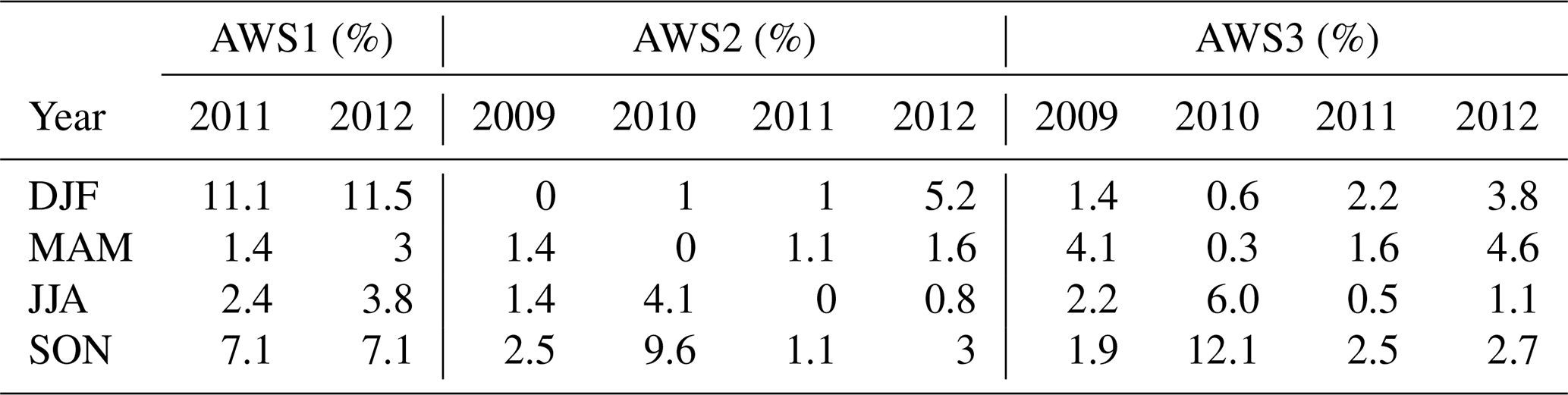
Föhn winds have been observed over the whole Larsen C Ice Shelf and are most frequent at the foot of the AP mountains (Elvidge et al., 2015; Turton et al., 2018; Wiesenekker et al., 2018). In certain seasons, föhn conditions can be observed up to 12 % of the time (Table 2). However, it is not uncommon to have a whole season without the occurrence of föhn conditions. They are most frequently observed in spring over the Larsen C Ice Shelf (AWS2 and AWS3) and more frequently in summer closer to the foot of the mountains (AWS1; Table 2). At all three locations in this study, the average 6-hourly temperature change associated with föhn events exceeds 11 K and the relative humidity decreases at least 19 % (Turton et al., 2018).
Table 2The percentage of time in which 6-hourly föhn conditions were identified from both AWS observations and AMPS. Values are taken from Turton et al. (2018) and presented here because the frequency of föhn conditions is important for the discussion. SON is spring; DJF is summer; MAM is autumn; and JJA is winter. Refer to Table 1 for information on data gaps. Percentages represent the ratios between föhn conditions and the total duration of non-missing data. December values are taken from the preceding year, to keep within the same melting season (for example DJF 2012 spans 1 December 2011 to 29 February 2012).
3.2 Surface melting in AMPS
In order to assess AMPS surface melt, we compare it to the observationally derived SEB at AWS2, for which data are available for the full 4-year period. Melt days in both AMPS and the SEB are defined as days when melting (Emelt>0) is observed. During 2009–2012 the SEB model identified 214 melt days (15 % of the time) at AWS2, compared to 289 for AMPS (20 % of the time; Table 3). AMPS therefore overestimates the number of melt days compared to observations, likely due to the overestimation of air temperature during non-föhn days in AMPS (Kirchgaessner et al., 2019).
Table 3The representation of surface melt from observation-derived data at AWS2, alongside AMPS model output interpolated to the same location. The total number of days with observations for 2009 to 2012 is 1439, which is used for the calculation of percentages for rows 2–4. The average Emelt values are daily averages over the same period. The total number of föhn and non-föhn days are the same for both AWS and AMPS as a result of the föhn identification (Sect. 2.4): föhn conditions must be identified in both to be classified as föhn. The number of föhn and non-föhn days are the same in AWS and AMPS as this was a criterion for the detection of föhn winds in Turton et al. (2018).
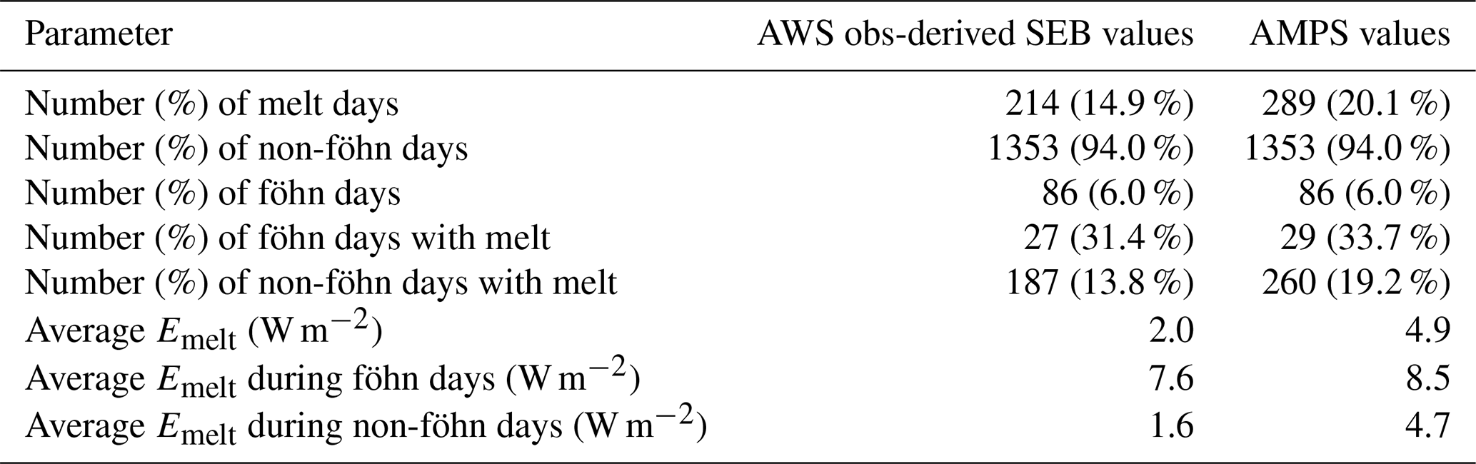
In both the observations and AMPS, over 30 % of föhn days observed at AWS2 lead to surface melt (Table 3). AMPS slightly overestimates the percentage of föhn days which experience melting but only by 2.3 % (2 d). However, AMPS overestimates the number of melt days coinciding with non-föhn days more considerably (260 non-föhn days experience melting in AMPS compared to 187 in observations). AMPS is therefore better able to represent the occurrence of melting on föhn days as opposed to melting on non-föhn days.
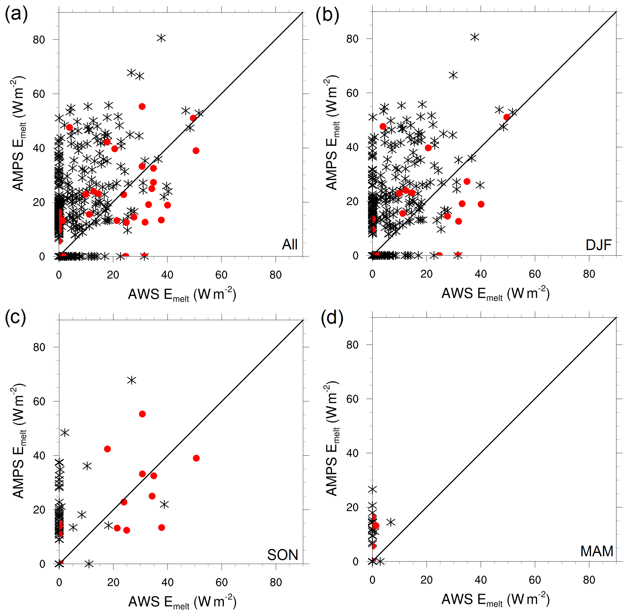
Figure 3Scatter plots of daily Emelt values (W m−2) from observations at AWS2 and AMPS during (a) all months, (b) summer (DJF), (c) spring (SON) and (d) autumn (MAM). Red dots indicate föhn days whilst black stars are non-föhn days.
Similarly, AMPS overestimates the average Emelt during non-föhn days but is more able to represent föhn days (Table 3 and Fig. 2). The largest overestimation occurs during non-föhn days, when AMPS simulates a mean Emelt of 4.7 W m−2 compared to 1.6 W m−2 in observationally derived values at AWS2. However, during föhn conditions, Emelt is better represented by AMPS, with a smaller positive bias of 0.9 W m−2 on average. This can also be seen in Fig. 2. AMPS simulates the largest Emelt values best and overestimates Emelt most during non-föhn days. When separating by season (Fig. 3), it is clear that AMPS overestimates Emelt in all seasons (except winter) but more often during summer. Some of the largest amounts of daily melting often coincide with föhn days during spring and summer (Fig. 3b, c), and AMPS is better able to represent events with large melt amounts than those with low melt rates. These results agree with findings by Kirchgaessner et al. (2019), who found that AMPS underestimates the air temperature during föhn days but overestimates the temperature the rest of the time, which leads to a higher surface temperature and a higher likelihood of melting on non-föhn days (Kirchgaessner et al., 2019). Figure 3c also highlights that the majority of melting during spring is associated with föhn days, which AMPS represents well.
The downwelling shortwave radiation is overestimated by AMPS for this location (King et al., 2015, 2017). Combined with the low albedo value and the poor representation of clouds in AMPS, the ice surface is much warmer in AMPS than in reality (mean bias of 1.8 K). Therefore, on days in late spring and summer when the skin temperature is close to the melting point in observations, AMPS will simulate temperatures at or near 0 ∘C, leading to an overestimation of the total number of melt days (Fig. 3a, b). An overestimation of melt days was also found in other studies using AMPS and the polar WRF model over ice shelves (Grosvenor et al., 2014; King et al., 2008, 2015; Kirchgaessner et al., 2019).
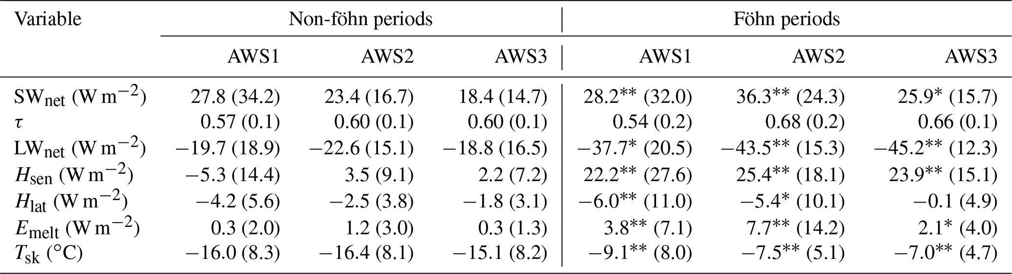
During föhn conditions, when the melt amount is better represented by AMPS, there are a number of reasons for the smaller positive bias in Emelt, alongside lower air temperatures (Kirchgaessner et al., 2019). AMPS overestimates the latent heat flux (Hlat). The observation-derived values of Hlat at AWS1, AWS2 and AWS3 during föhn composites are −6.2, −3.6 and −1.3 W m−2 respectively (Fig. 4e). AMPS simulated Hlat values of −24.4, −10.6 and −10.9 W m−2 for the AWS1, AWS2 and AWS3 locations respectively, during föhn conditions. AMPS also overestimates the net longwave flux (LWnet) during föhn conditions but with much smaller biases than for Hlat. During föhn conditions, AMPS simulates an average LWnet of −36.1 W m−2 for AWS1, −43.0 W m−2 for AWS2 and −43.7 W m−2 for AWS3. From the observation-derived SEB values, AWS1, AWS2 and AWS3 have LWnet values of −34.8, −40.6 and −41.1 W m−2 during föhn conditions respectively (Fig. 4e). A combination of lower (more negative) LWnet and Hlat during föhn days in the simulations acts to cool the surface more than is observed, which could be responsible for the better representation of Emelt during föhn days compared to non-föhn days in AMPS.
Regardless of the overestimation of non-föhn melt in AMPS, it is evident from the observations and AMPS that melting during föhn conditions is significantly higher (p value of p<0.01 from t test) during föhn conditions than during non-föhn conditions, even at more than 100 km away from the foot of the AP mountains. As AMPS is able to reproduce föhn-related melting, we have used it to assess the spatial distribution of föhn-induced melting for the entire ice shelf (Fig. 5). Föhn-induced melting is most frequent in the north of the ice shelf, largely mirroring the spatial distribution of föhn conditions and the near-surface air temperature (Turton et al., 2018). During summer, föhn-induced melting is simulated over the whole area from Scar Inlet in the north across the entire Larsen C Ice Shelf to 70∘ S. Outside of summer, föhn-induced melting is still prevalent over the ice shelf, with over forty 6-hourly melt events simulated on Scar Inlet during spring (Fig. 5b). There are more föhn-induced melt events during spring than in autumn, likely related to the higher occurrence of föhn during spring.
The following analysis, separated into the annual, interannual and seasonal impact of föhn, uses the observations and derived SEB components at the three locations to quantify the impact of föhn on the ice shelf.
3.3 Annually averaged impact of föhn
Figure 4 presents the annually averaged differences between föhn and non-föhn conditions for the observed SEB components. In the SEB data, 14 % of non-föhn days at AWS2 from 2009 to 2012 are melt days. These are largely confined to summer months, when melting occurs annually. The frequency of melt days more than doubles when assessing föhn days, with 31 % of föhn days at AWS2 coinciding with melt days. A similar magnitude of increase is observed at AWS3, where melt-day occurrence increased from 12 % during non-föhn conditions to 20 % during föhn days. Therefore, even at a distance of 100 km from the foot of the mountains, föhn conditions are able to increase the number of melt days per year. The largest increase in melt-day occurrence is at AWS1, where the percentage of days observing melt increases from 14 % during non-föhn days to 43 % during föhn days in 2011 and 2012.
During föhn conditions incoming shortwave radiation (SW↓) is hypothesised to be larger due to the clearance of clouds, which can occur in the lee of the AP mountains (Grosvenor et al., 2014; Elvidge and Renfrew, 2016). However, due to the large annual cycle in SW↓ in the polar regions, the seasonal magnitude of SW↓ could bias the difference between föhn and non-föhn days if they are not evenly distributed throughout the year. As shown in Table 2 and Turton et al. (2018), föhn days are not evenly distributed seasonally or interannually. Therefore, the shortwave transmissivity (τ; see “Data”) is a more reliable indication of the impact of föhn winds on the downwelling shortwave radiation. Data show an increase in shortwave transmissivity at all three locations during föhn conditions, indicating an increase in the incoming shortwave radiation due to cloud clearance (Fig. 4a). However, the differences in τ between föhn and non-föhn conditions are small and are non-significant.
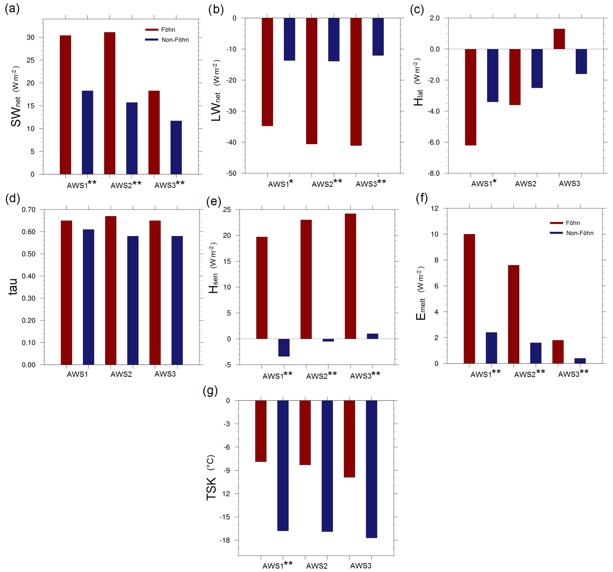
Figure 4The mean shortwave net radiation (a), longwave net radiation (b), latent heat flux (c), τ (d), sensible heat flux (e), Emelt (f) and skin temperature (g) from the three locations during all föhn (red) and non-föhn (blue) periods from 2009 to 2012. * indicates a statistically significant difference between non-föhn and föhn values at the 95 % confidence level using the t test, and ** indicates the same at the 99 % confidence level. Differences were not assessed for τ, derived from the average SW and SWtop, owing to small sample size.
The sensible heat flux (Hsen) is much larger (and more positive) during föhn conditions than during non-föhn conditions (Fig. 4d). This is due to the increased air temperature and higher wind speed, both leading to an increased supply of heat to the surface. The mean annual average sensible heat fluxes, observationally derived during föhn days at AWS2 and AWS3, are very similar (23.0 and 24.2 W m−2 respectively; Fig. 4d). However, at AWS1 sensible heat fluxes are slightly smaller (19.7 W m−2) than at the other locations due to the slightly lower wind speeds under föhn conditions at this location compared to the other locations. In most locations along the foot of the AP, the wind speeds are higher than further downstream. However, for the 2 years of available data at AWS1, this is not the case here. Despite the smaller Hsen value at AWS1, the increase in Hsen between non-föhn and föhn days is similar to the other locations: between 23.1 W m−2 at AWS1 and 23.5 W m−2 at AWS2. The high Hsen during föhn conditions impacts all of the Larsen ice shelves, with 25 W m−2 values simulated over all of Larsen B and C ice shelves (Fig. 6d). Very close to the foot of the AP mountains, AMPS simulates higher Hsen values, where föhn conditions are stronger in the inlets and föhn-induced melting can also occur in winter (Kuipers Munneke et al., 2018).
The latent heat flux becomes more negative during föhn days at AWS1 and AWS2, which we can attribute to the increase in sublimation of surface snow increases due to the dry air over the ice shelf (Fig. 6). At AWS3, there is an increase in Hlat (1.3 W m−2) during föhn conditions, although the differences with non-föhn conditions are not statistically significant. At AWS1, the difference in Hlat between föhn and non-föhn conditions is larger than at the other locations and is significant. This is likely due to the drier föhn conditions observed close to the AP, whereas at about 100 km distance, the air has become moister due to mixing with pre-existing non-föhn air, and therefore less sublimation occurs. This is evident in the AMPS simulation (Fig. 6), with more negative values of Hlat closer to the AP during föhn days.
LWnet becomes significantly more negative during föhn events (Fig. 4c), which is likely related to the “föhn clearance”, whereby fewer clouds during föhn conditions lead to a reduced downwelling flux of longwave radiation (Elvidge and Renfrew, 2016). Simultaneously, the warmer surface increases the outgoing longwave radiation flux, and both of these factors contribute to a more negative LWnet than during non-föhn conditions. Despite the larger negative fluxes of LWnet and Hlat during föhn conditions, the positive increase in SWnet and Hsen contributes to more energy being available for melt (Emelt) during föhn conditions.
Emelt more than triples during föhn conditions compared to non-föhn conditions, from 1.6 to 7.6 W m−2 at AWS2 and from 2.4 to 10.0 W m−2 at AWS1 (Fig. 4f). AWS1 is closer to the foot of the AP mountains and therefore experiences warmer and more frequent föhn conditions, which contributed to the significantly higher amount of energy available for melt during föhn periods. Figure 6 presents a spatial distribution of the energy flux during föhn periods in AMPS. A higher energy flux is present over Larsen B than Larsen C during föhn winds.
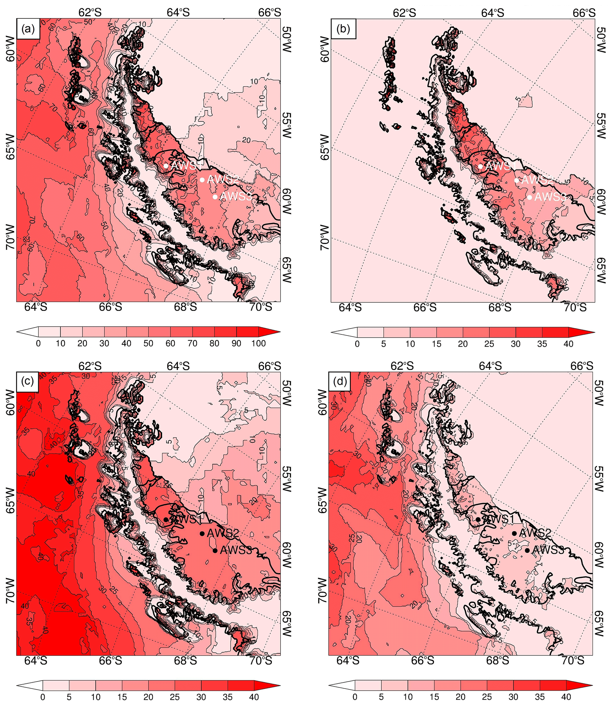
Figure 5The number of 6-hourly melt events in AMPS during all föhn events (a), spring (b), summer (c) and autumn (d). Winter is not included as there were no melt days simulated by AMPS.
3.4 Interannual melt
Due to the poor availability of data at the AWS1 and AWS3 locations, this section focuses solely on AWS2 data. Mean annual melt from 2009 to 2012 (föhn and non-föhn conditions combined) is 180 mm w.e. yr−1 at AWS2. Excluding föhn days, the annual average melt amount at AWS2 reduces significantly to 146 mm w.e. yr−1. In other words, föhn increases the melt volume at AWS2 by 34 mm w.e. yr−1 (18 %). The majority of non-föhn melting is restricted to the summer months.
The influence of föhn winds on surface melt is largest in the years with a large number of föhn conditions during the early spring–summer period (September–December). The year 2010 was exceptional in this regard, with thirty-five 6-hourly föhn conditions identified at AWS2 alone. For comparison, the number of identified föhn conditions at AWS2 from September to December in 2009, 2011 and 2012 were 12, 13 and 11 respectively. The annual melt amount at AWS2 in 2010 was 258 mm w.e. This annual total decreases by 76 to 182 mm w.e. when the melt associated with föhn conditions is removed. Focusing specifically on spring (SON) 2010, there were 22 föhn days, of which 11 of them generated melting (50 %) at AWS2. Conversely, there were 69 non-föhn days in spring 2010 (AWS2), of which just 8 d experienced melting (12 %). King et al. (2017) studied the impact of the föhn conditions in November 2010 in more detail and identified that the duration and frequency of melting over Larsen C increased due to föhn winds in this period.
In contrast to 2010, only 11 föhn conditions were identified at AWS2 from September to December in 2012. The annual melt amount in 2012 was 83 mm (significantly less than in 2010 at the 95 % level). When föhn days were removed from the 2012 analysis, the annual total melt only decreased by 0.1 mm w.e. During spring, little melt is observed except on föhn days. Hence, the frequency of föhn winds in spring has an impact on the melt and can extend the melt season.
The annual number of melt days, energy available for melt, annual melt amount and length of the melt season all increased due to the occurrence of föhn winds, especially in years when a large number of föhn conditions were identified during the extended summer period (October–March). We will now present the impact of föhn winds in separate seasons but with a particular focus on spring.
3.5 Spring
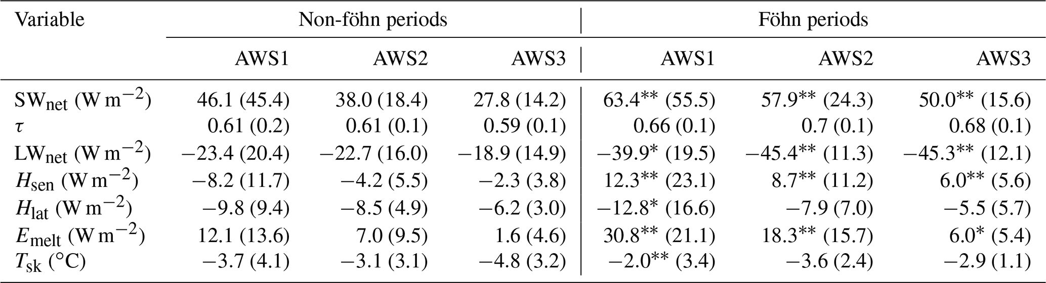
The largest increase in surface melting is associated with springtime föhn events (SON). Although not all changes in mean values between non-föhn and föhn conditions were statistically significant, the changes in the SEB indicate a large impact due to föhn winds. Table 4 displays the average values for composites of föhn and non-föhn periods during spring.
Table 4Spring daily averages of surface temperature and SEB components for föhn and non-föhn conditions. In brackets are the standard deviations for each field.
* A statistically significant difference between föhn and non-föhn periods using the t test at the 95 % confidence level. A statistically significant difference between föhn and non-föhn periods using the t test at the 99 % confidence level.
The atmospheric transmissivity (τ) increases during föhn conditions indicating an increase in incoming shortwave radiation at the surface, although not statistically significantly. The net longwave radiation is significantly lower during föhn conditions than during non-föhn conditions at all locations (p<0.05; Table 4). Both turbulent fluxes exhibited significant differences during föhn conditions compared to non-föhn conditions at AWS1 and AWS2. The sensible heat flux increases (more positive) by over 20 W m−2 at all locations (Table 4), and the largest increase is observed at AWS1 (27.5 W m−2). The warmer air and higher wind speeds contribute significantly to increasing Hsen over the ice shelf. The latent heat flux is more negative at AWS1 and AWS2 during föhn conditions, indicative of sublimation and evaporation. However, at AWS3 Hlat increases, although this was not statistically significant (p value <0.05; Table 4).
The cooling effect of the net longwave radiation and latent heat flux is not large enough to counteract the considerable heating processes; therefore, melt energy is available during spring föhn conditions. At AWS2 during spring, melting occurs on just 3 % of non-föhn days, due to the low temperatures in the absence of föhn winds. However, melting increases significantly when accounting for föhn conditions. In spring, 28 % of föhn days coincide with observed melting. A similar increase was found during föhn days at the other locations: at AWS1 just 5 % of non-föhn days coincide with melt days, whilst 30 % of föhn-days coincide with melt days. At AWS3, 4 % of non-föhn days and 28 % of föhn days experience melting.
At AWS2, the average energy available for melt (Emelt) during spring föhn conditions is 7.7 W m−2 (Fig. 7). This is greater than the mean daily melt energy during summer at this location (7.0 W m−2). The amount of melt energy associated with föhn conditions at AWS1 is lower (3.8 W m−2) than at AWS2; however this does not take into account the large melt amount and early melt onset associated with föhn winds in spring 2010, as data are only available from February 2011 to December 2012. When assessing the annual average melt energy for 2012 (period in which observations overlap), there is considerably more daily melt energy at AWS1 (3.5 W m−2) than at AWS2 (1.0 W m−2).
Therefore, during spring, föhn conditions increase both the average rate of melt production and the number of melt days, both close to the foot of the AP and up to 130 km away.
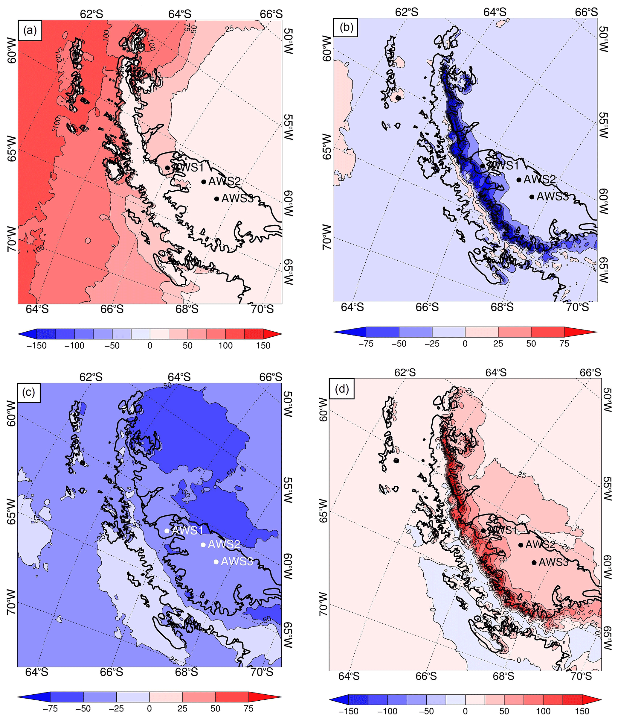
Figure 6The energy (a), latent heat (b), net longwave (c) and sensible heat (d) fluxes as a composite of all föhn events from 2009–2012 in AMPS.
3.6 Summer
The energy available for melt and percentage of melt days during summer are relatively high, regardless of additional föhn-induced melting, due to higher air temperatures and larger SW↓ during this season (Fig. 7, Table 5). A day may already have experienced melting, and the presence of föhn winds was coincidental and did not cause the melting. However, from case studies, it has been found that individual föhn events can increase or prolong melt when it occurs during summer (Elvidge et al., 2016; Kuipers Munneke et al., 2012).
Table 5Summer daily average values of SEB components and surface temperature during composites of föhn and non-föhn conditions at AWS1, AWS2 and AWS3. In brackets are the standard deviations for each field.
* Statistically significant differences between föhn and non-föhn periods using the t test at the 95 % confidence level. Statistically significant differences between föhn and non-föhn periods using the t test at the 99 % confidence level.
There is a significant increase in the net shortwave radiation and a decrease in net longwave radiation during summer föhn periods in comparison to non-föhn conditions, likely due to the cloud clearing during föhn (Table 5; Grosvenor et al., 2014). The sensible heat flux significantly increases at all three locations during föhn conditions, which changes the direction of energy transport from negative (away from the surface) during non-föhn to positive (downwards) during föhn conditions. Negative sensible heat flux, associated with convection, is common at AWS2 during summer (Kuipers Munneke et al., 2012).
As a consequence of the higher surface temperatures, sublimation and evaporation are common in summer, leading on average to a negative latent heat flux. Under föhn conditions, the change in conditions is mixed. At AWS1, the latent heat flux becomes more negative during föhn conditions, indicative of enhanced sublimation (Table 5). At AWS2 and AWS3, Hlat increases; however the changes from non-föhn to föhn are not significant.
The increase in Emelt during föhn conditions is statistically significant at all locations and is largest at AWS2 (95 % confidence level), increasing from 7.0 to 18.3 W m−2. During 78 % of föhn days the surface is melting, compared to just 54 % of non-föhn summer days (at AWS2). The number of melt days and the melt energy both increase in summer under föhn conditions. Despite the already warm conditions and high melt amount, there are statistically significant changes to the SEB components and melt energy due to föhn conditions in summer.
Table 6Melt onset and end dates. Melt onset refers to the first day with observed melting. Melt end is the last day of the melt season on which melt is observed. Dates are taken from AWS2 to allow comparison with Luckman et al. (2014) melt onset and end dates. A range of values are given due to the uncertainty of reading Fig. 2 from Luckman et al. (2014) and are not the variation in dates.
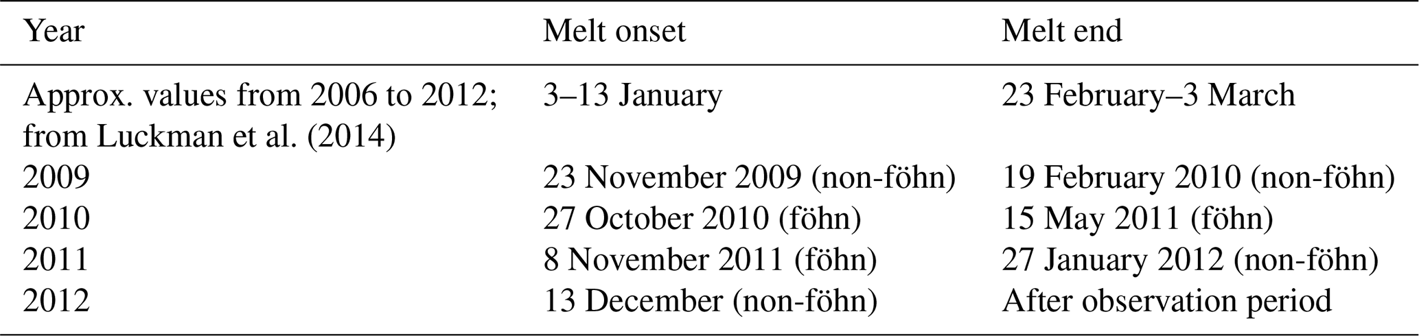
Luckman et al. (2014) presented the average melt onset and end dates from 2006 to 2012 for the Larsen C Ice Shelf, taken from satellite radar backscatter observations. At the location of AWS2, the approximate start and end dates of the melting season are provided in Table 6. The earliest onset of a melting season (in 2009–2012) was on 27 October 2010, which was associated with a föhn event. Similarly, the end of the melt season was associated with föhn-induced melting observed on 15 May 2011. This is far outside of the typical melt season at this location. The preceding melt day was on 5 March 2011 and was not associated with föhn winds. Therefore, föhn winds have the ability to induce melting outside of the usual summer melt period.
3.7 Autumn
The sensible heat flux is positive and significantly larger during föhn days in all three locations and in AMPS output (not shown). On average, Hsen increases from 0.0 W m−2 during non-föhn periods to 20.9 W m−2 during föhn conditions at AWS2. This agrees well with the AMPS output, which simulates a mean Hsen of 24.9 W m−2 during föhn days in autumn at AWS2. Surface warming is also significantly larger during föhn days than during non-föhn days, raising the surface temperature by 11.8 K at AWS2.
Figure 3d highlights the low daily Emelt values at AWS2 during autumn. The energy available for melt only increases by 0.1 W m−2 (at AWS2) between föhn and non-föhn days. Melting only occurs on 1 % of non-föhn days, whereas 8 % of föhn days experience melting at AWS2. Closer to the AP, föhn-induced melting is higher than at the stations further east. The percentage of föhn days experiencing melt at AWS1 is 43 % compared to just 1 % of non-föhn days. Daily average Emelt increased from 0 W m−2 during non-föhn days to 4.3 W m−2 during föhn days. Therefore, föhn-induced melting is possible during autumn, although it is limited in extent and only occurs very close to foot of the AP mountains, where föhn winds are warmer.
3.8 Winter
The smallest impact from föhn conditions on surface melt was observed during winter. The radiation deficit in winter, mainly due to the lack of solar radiation, is so large that increased sensible heat during föhn can almost never bring the surface to the melting point, except in the inlets of the AP (Kuipers Munneke et al., 2018). There was no melting observed at any AWS location (or anywhere on the ice shelf in the AMPS output) during winter between 2009 and 2012. Nonetheless, föhn does have an impact on the individual SEB components during winter, as the air temperature can often rise above freezing (Kirchgaessner et al., 2019).
Hsen and Hlat both experience a significant change between föhn and non-föhn days. At AWS2 the average Hsen increases from 3.4 to 36.6 W m−2 during föhn days and the latent heat increases from 0.6 to 2.9 W m−2. A similar magnitude of change in Hsen and Hlat is observationally derived at AWS3 and AWS1. The large increase in Hsen is attributed to the considerably warmer (and often windier) conditions during föhn. There is no observation-derived melting during winter föhn events at the locations we have shown.
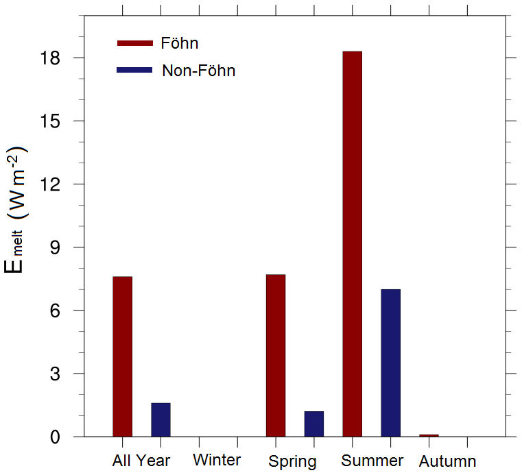
Figure 7The observationally derived melt energy Emelt values from AWS2 during föhn and non-föhn conditions, separated by seasons.
This study used three locations for SEB calculation from observations, to provide a larger spatial interpretation of melting associated with föhn winds. Observations and the SEB model were available on the remnants of the Larsen B Ice Shelf from February 2011 to December 2012 and have shown evidence of föhn-induced melting close to the AP. This is the first time that the results from the SEB model have been analysed and presented for Larsen B (AWS1). More recently, data have become available for more locations on Larsen C, including the inlets, which observe high melt rates associated with föhn winds (Kuipers Munneke et al., 2018).
The large increase in melt energy, number of melt days and increased duration of melting during spring are likely the biggest impacts of föhn conditions on the surface of the Larsen Ice Shelf. This föhn-induced melting at AWS2 during spring is comparable in energy and melt amount to that of non-föhn conditions in summer. In the absence of föhn conditions in spring, the melt amount is significantly smaller. In one particular melt season of 2010/11, the melt season was 164 d long due to an early onset on 27 October 2010 and a late end date of 15 May 2011. This is a much longer melt period than was observed at this location between 2009 and 2012. Luckman et al. (2014) published melt duration, melt onset and melt end dates for the Larsen C Ice Shelf from 2006 to 2012 and showed the average melt duration for Larsen C is 50–60 d. Therefore, föhn winds can significantly extend the melt duration. Prior to the current study, our understanding of the impact of föhn winds on the SEB of Larsen C was limited to a number of case studies.
During the period under investigation in this study there were no melt days on either föhn or non-föhn days during winter at the three AWS locations. There is a high spatial and temporal variability in the occurrence and strength of föhn winds over Larsen C (Elvidge et al., 2015, 2016; Turton et al., 2018), which likely explains the contradicting results of Kuipers Munneke et al. (2018), who identified high rates of winter melting associated with föhn winds in 2016. The winter melting period investigated previously was not within the period investigated here. Unfortunately, SEB data at the foot of the AP (AWS1) were only available for a limited period, when the largest melt rate and highest number of melt days were previously observed in satellite images (Luckman et al., 2014). With a longer observational period at AWS1 now available, this site should be investigated further, as winter melt may be specific to individual years.
The number of melt days estimated by AMPS exceeded the observationally derived values during non-föhn days. One reason for the melt-day overestimation is the positive bias in near-surface temperature during non-föhn conditions in AMPS (Kirchgaessner et al., 2019). This is caused by the positive bias in incoming shortwave radiation, which results from the poor representation of clouds in the model (Listowski and Lachlan-Cope, 2017), together with the low albedo value used in AMPS. This has been discussed by Grosvenor et al. (2014) and King et al. (2015, 2017). As a result, values of melt energy currently derived from AMPS cannot be trusted if used as an absolute estimate of melting specifically caused by föhn winds. However, they can be used to infer the spatial patterns of melting during föhn days and the average melt energy when including all melt events. The poor representation of clouds in many regional climate models causes issues in the accuracy of SEB and melt information. Recently, Gilbert et al. (2020) found that the cloud phase during the austral summer strongly influences the amount of melting on the Larsen C Ice Shelf and can determine whether melting is simulated or not by the UK Met Office Unified Model (MetUM).
Another reason for the positive bias in melt amount during non-föhn periods in AMPS is due to the overestimation of föhn periods. In Turton et al. (2018), föhn conditions were identified from both AWS and AMPS output separately, but“föhn” was only considered and analysed further when it was simultaneously identified in both datasets. Between 2009 and 2012, AMPS overestimated the number of föhn periods identified compared to AWS observations. These were not classified as föhn periods in the current study but may have föhn characteristics (higher temperatures and lower relative humidity) which did not quite meet the thresholds set by Turton et al. (2018). Therefore, some overestimation in non-föhn melt days could be because the model simulates a föhn event, which was not observed.
Satellites can provide a longer-term perspective for the period 2009–2012 that we study here. According to QuikSCAT, the number of melt days was particularly low in the 2009–2010 and 2012–2013 summer seasons (Bevan et al., 2018). The 2010–2011 and 2011–2012 summer seasons have longer melt periods; however in the context of the last 18 years, they were not considered high-melt years (Bevan et al., 2018). The spatial pattern of melting in these two seasons had a bimodal melting pattern, where the northern section of Larsen C had a higher number of melt days (60–75 d) than the southern part of Larsen C (10–25 melt days; Bevan et al., 2018). Whilst the three observational sites used in the current study are in the higher-melt zone, there were relatively fewer föhn events in the 2009–2012 period than during other periods between 1999 and 2017 used in Bevan et al. (2018). This was corroborated by Datta et al. (2019), who used microwave satellite data to assess melt duration over the northern Antarctic Peninsula between 1982 and 2017. They found periods of high melting associated with föhn winds during the 1990s (Datta et al., 2019). Therefore, the effects of föhn winds on the SEB could be even greater than we have highlighted in this study if the SEB could be calculated for particularly high-melt years.
The discrimination between föhn and non-föhn conditions over a 4-year period provides a robust understanding of the impact of föhn on components of the SEB and, ultimately, surface melt. Furthermore, by assessing the more general response to föhn, as opposed to individual events, we now know the impact of particularly frequent föhn periods on the surface melt. The limitation of assessing case studies is that the chosen event may be an anomaly or not representative of the average föhn conditions. Here, we have assessed the average impact of föhn events to provide more confidence in the quantification of surface melt due to föhn.
Particularly in spring, föhn conditions have the potential to prolong the melt season by initialising an early onset of the melt season. Previously, King et al. (2017) identified the importance of springtime föhn winds in a particular season. We have subsequently extended that study to include four spring seasons and conclude that the intensity of melt increases during föhn conditions, even 100 km from the AP. However, the strength of the SEB impact depends on the frequency of föhn winds in spring. Spring 2010 saw a clustering of föhn winds which caused the biggest increase in surface melting in the 4-year period. Föhn conditions have a large impact on the sensible heat flux, which leads to an excess of energy that is available to heat and melt the snow during spring, summer and, occasionally, autumn.
The strengths and weaknesses of AMPS in representing the meteorological characteristics of föhn winds and their identification in model output were investigated by Turton et al. (2018) and Kirchgaessner et al. (2019). Similarly, King et al. (2015) compared AMPS to observations of SEB for a 1-month summertime period in January 2011. However, the suitability of AMPS for evaluating the föhn-induced melting over Larsen C had not been tested. Here we present the representation of year-round SEB, surface melting and föhn-induced surface melting in AMPS compared to AWS2 observations. AMPS is more capable of accurately simulating surface melt during föhn periods than during non-föhn periods (Table 3), especially during spring (Fig. 3c). Similarly, AMPS performs well at simulating the number of föhn-induced melt days (29 compared to 27 in observations). Non-föhn values of Emelt are overestimated by 3.1 W m−2 compared to just 0.9 W m−2 during föhn periods, and the number of non-föhn melt days is also higher in AMPS than in observations (260 compared to 187). The overestimation of non-föhn melting is likely due to the higher negative biases in net longwave radiation and latent heat flux and not due to a good representation of föhn warming. Therefore, to completely trust the impact of föhn winds on the SEB of the Larsen C Ice Shelf, the components of the SEB should be improved in AMPS.
Subsets of the AMPS output are available online at https://www.earthsystemgrid.org/search.html?Project=AMPS (last access: 17 November 2020). The surface energy balance values from AWS1, AWS2 and AWS3 are available upon request from Peter Kuipers Munneke at p.kuipersmunneke@uu.nl.
Analysis of the SEB and AMPS data was undertaken by JVT, AK and JCK. The author PKM ran the SEB model and provided discussion of the results. JVT, AK and ANR contributed to the development of the research question. All authors contributed to the progress of the manuscript and the discussion of the results.
The authors declare that they have no conflict of interest.
The authors would like to acknowledge the Natural Environment Research Council (NERC) UK grant NE/G014124/1 “Orographic flows and the climate of the Antarctic Peninsula” and NERC-funded PhD studentship NE/L501633/1. We acknowledge the National Center for Atmospheric Research (NCAR), USA, for access to the archived AMPS output. We also appreciate the work of IMAU, CIRES and the British Antarctic Survey staff at Rothera station for their field support. Thank you to our editor, Elizabeth Bagshaw; the anonymous reviewer; and Jan Lenaerts for their reviews and suggestions to improve the manuscript.
This research has been supported by the Natural Environment Research Council (grant nos. NE/L501633/1 and NE/G014124/1).
This paper was edited by Elizabeth Bagshaw and reviewed by Jan Lenaerts and one anonymous referee.
Antarctic Mesoscale Prediction System (AMPS), Mesoscale and Microscale Meteorology (MMM) laboratory, National Center for Atmospheric Research: https://www.earthsystemgrid.org/project/amps.html, last access: 17 November 2020.
Bell, R. E., Banwell, A. F., Trusel, L. D., and Kingslake, J.: Antarctic surface hydrology and impacts on ice-sheet mass balance, Nat. Clim. Change, 8, 1044–1052, 2018.
Bevan, S. L., Luckman, A. J., Kuipers Munneke, P., Hubbard, B., Kulessa, B., and Ashmore, D. W.: Decline in surface melt duration over Larsen C ice shelf revealed by the Advanced Scatterometer (ASCAT), Earth Space Sci., 5, 578–591, 2018.
Brandt, R. E. and Warren, S. G.: Solar-heating rates and temperature profiles in Antarctic snow and ice, J. Glaciol., 39, 99–110, 1993.
Cape, M. R., Vernet, M., Skvarca, P., Marinsek, S., Scambos, T., and Domack, E.: Foehn winds link climate-driven warming to ice shelf evolution in Antarctica, J. Geophys. Res.-Atmos., 120, 11037–11057, 2015.
Datta, R. T., Tedesco, M., Fettweis, X., Agosta, C., Lhermitte, S., Lenaerts, J. T. M., and Wever, N.: The effects of Foehn-induced surface melt on firn evolution over the northeast Antarctic Peninsula, Geophys. Res. Lett., 46, 3822–3831, 2019.
Doake, C. S. M., Corr, H. F. J., Rott, H., Skvarca, P., and Young, N. W.: Breakup and conditions for stability of the northern Larsen ice shelf, Antarctica, Nature, 391, 778–780, 1998.
Elvidge, A. D. and Renfrew, I. A.: The causes of foehn warming in the lee of mountains, B. Am. Meteorol. Soc., 97, 455–466, 2016.
Elvidge, A. D., Renfrew, I. A., King, J. C., Orr, A., Lachlan-Cope, T. A., Weeks, M., and Gray, S. L.: Foehn jets over the Larsen C ice shelf, Antarctica, Q. J. Roy. Meteor. Soc., 141, 698–713, 2015.
Elvidge, A. D., Renfrew, I. A., King, J. C., Orr, A., and Lachlan-Cope, T. A.: Foehn warming distributions in nonlinear and linear flow regimes: a focus on the Antarctic Peninsula, Q. J. Roy. Meteor. Soc., 142, 618–631, 2016.
Gilbert, E., Orr, A., King, J. C., Renfrew, I. A., Lachlan-Cope, T., Field, P. F., and Boutle, I. A.: Summertime cloud phase strongly influences surface melting on the Larsen C ice shelf, Antarctica, Q. J. Roy. Meteor. Soc., 146, 1575–1589, https://doi.org/10.1002/qj.3753, 2020.
Grosvenor, D. P., King, J. C., Choularton, T. W., and Lachlan-Cope, T.: Downslope föhn winds over the Antarctic Peninsula and their effect on the Larsen ice shelves, Atmos. Chem. Phys., 14, 9481–9509, https://doi.org/10.5194/acp-14-9481-2014, 2014.
Hogg, A. E. and Gudmundsson, G. H.: Impacts of the Larsen-C ice shelf calving event, Nat. Clim. Change, 7, 540–542, 2017.
King, J. C., Lachlan-Cope, T. A., Ladkin, R. S., and Weiss, A.: Airborne measurements in the stable boundary layer over the Larsen Ice shelf, Antarctica, Bound.-Lay. Meteorol., 127, 413–428, 2008.
King, J. C., Gadian, A., Kirchgaessner, A., Kuipers Munneke, P., Lachlan-Cope, T. A., Orr, A., Reijmer, C., van den Broeke, M. R., van Wessem, J. M., and Weeks, M.: Validation of the summertime surface energy budget of Larsen C ice shelf (Antarctica) as represented in three high-resolution atmospheric models, J. Geophys. Res.-Atmos., 120, 1335–1347, 2015.
King, J. C., Kirchagessner, A., Orr, A., Luckman, A., Bevan, S., Elvidge, A., Renfrew, I., and Kuipers Munneke, P.: The impact of foehn winds on surface energy balance during the 2010–2011 melt season over Larsen C ice shelf, Antarctica, J. Geophys. Res.-Atmos., 122, 12062–12076, 2017.
Kirchgaessner, A., King, J. C., and Gadian, A.: The representation of Föhn events to the east of the Antarctic Peninsula in simulations by the Atmospheric Mesoscale Prediction System, J. Geophys. Res.-Atmos., 124, 13663–13679, 2019.
Kuipers Munneke, P., van den Broeke, M. R., Reijmer, C. H., Helsen, M. M., Boot, W., Schneebeli, M., and Steffen, K.: The role of radiation penetration in the energy budget of the snowpack at Summit, Greenland, The Cryosphere, 3, 155–165, https://doi.org/10.5194/tc-3-155-2009, 2009.
Kuipers Munneke, P., van den Broeke, M. R., King, J. C., Gray, T., and Reijmer, C. H.: Near-surface climate and surface energy budget of Larsen C ice shelf, Antarctic Peninsula, The Cryosphere, 6, 353–363, https://doi.org/10.5194/tc-6-353-2012, 2012.
Kuipers Munneke, P., Luckman, A. J., Bean, S. L., Smeets, C. J. P. P., Gilber, E., van den Broeke, M. R., Wang, W., Zender, C., Hubbard, B., Ashmore, D., Orr, A., King, J. C., and Kulessa, B.: Intense winter surface melt on an Antarctic ice shelf, Geophys. Res. Lett., 45, 7615–7623, 2018.
Leeson, A. A., van Wessem, M., Ligtenberg, S., Shepherd, A., van den Broeke, M., Killick, R. C., Skvarca, P., Marinsek, S., and Colwell, S.: Regional climate of the Larsen B embayment 1980–2014, J. Glaciol., 63, 683–690, 2017.
Listowski, C. and Lachlan-Cope, T.: The microphysics of clouds over the Antarctic Peninsula – Part 2: modelling aspects within Polar WRF, Atmos. Chem. Phys., 17, 10195–10221, https://doi.org/10.5194/acp-17-10195-2017, 2017.
Luckman, A., Elvidge, A., Jansen, D., Kulessa, B., Kuipers Munneke, P., King, J. C., and Barrand, N. E.: Surface melt and ponding on Larsen C ice shelf and the impact of föhn winds, Antarct. Sci., 26, 625–635, 2014.
Marshall, G. J., Orr, A., van Lipzig, N. P. M., and King, J. C.: The impact of a changing Southern Hemisphere annular mode on Antarctic Peninsula summer temperatures, J. Climate, 19, 5388–5404, 2006.
Powers, J. G., Manning, K. W., Bromwich, D. H., Cassano, J. J., and Cayette, A. M.: A decade of Antarctic science support through AMPS, B. Am. Meteorol. Soc., 93, 1699–1712, 2012.
Rignot, E., Casassa, G., Gogineni, P., Krabill, W., Rivera, A. and Thomas, R.: Accelerated ice discharge from the Antarctic Peninsula following the collapse of Larsen B ice shelf, Geophys. Res. Lett., 31, L18401, https://doi.org/10.1029/2004GL020697, 2004.
Robel, A. and Banwell, A. F.: A speed limit on ice shelf collapse through hydrofracture, Geophys. Res. Lett., 46, 12092–12100, 2019.
Scambos, T. A.: Glacier acceleration and thinning after ice shelf collapse in the Larsen B embayment, Antarctica, Geophys. Res. Lett., 31, L18402, https://doi.org/10.1029/2004GL020670, 2004.
Scambos, T. A., Hulbe, C., Fahnestock, M., and Bohlander, J.: The link between climate warming and break-up of ice shelves in the Antarctic Peninsula, J. Glaciology, 33, 945–958, 2000.
Trusel, L. D., Frey, K. E., Das, S. B., Kuipers Munneke, P., and van den Broeke, M. R.: Satellite-based estimates of Antarctic surface meltwater fluxes, Geophys. Res. Lett., 40, 6148–6153, 2013.
Trusel, L. D., Frey, K. E., Das, S. B., Karnauskas, K. B., Kuipers Munneke, P., van Meijgaard, E., and van den Broeke, M. R.: Divergent trajectories of Antarctic surface melt under two twenty-first century climate scenarios, Nat. Geosci., 8, 927–932, 2015.
Turton, J. V., Kirchgaessner, A., Ross, A. N., and King, J. C.: The spatial distribution and temporal variability of föhn winds over the Larsen C ice shelf, Antarctica, Q. J. Roy. Meteor. Soc., 144, 1169–1178, 2018.
van den Broeke, M. R., van As, D., Reijmer, C. H., and van de Wal, R. S. W.: Assessing and improving the quality of unattended radiation observations in Antarctica, J. Atmos. Ocean. Tech., 21, 1417–1431, 2004.
Van den Broeke, M.: Strong surface melting preceded collapse of Antarctic Peninsula ice shelf, Geophys. Res. Lett., 32, L12815, https://doi.org/10.1029/2005GL023247, 2005.
Wiesenekker, J., Kuipers Munneke, P., van den Broeke, M., and Smeets, C.: A multidecadal analysis of föhn winds over Larsen C ice shelf from a combination of observations and modelling, Atmospheres, 9, 172, https://doi.org/10.3390/atmos9050172, 2018.