Small-scale spatial variability in bare-ice reflectance at Jamtalferner, Austria

As Alpine glaciers become snow-free in summer, more dark, bare ice is exposed, decreasing local albedo and increasing surface melting. To include this feedback mechanism in models of future deglaciation, it is important to understand the processes governing broadband and spectral albedo at a local scale. However, few in situ reflectance data have been measured in the ablation zones of mountain glaciers. As a contribution to this knowledge gap, we present spectral reflectance data (hemispherical–conical–reflectance factor) from 325 to 1075 nm collected along several profile lines in the ablation zone of Jamtalferner, Austria. Measurements were timed to closely coincide with a Sentinel-2 and Landsat 8 overpass and are compared to the respective ground reflectance (bottom-of-atmosphere) products. The brightest spectra have a maximum reflectance of up to 0.7 and consist of clean, dry ice. In contrast, reflectance does not exceed 0.2 for dark spectra where liquid water and/or fine-grained debris are present. Spectra can roughly be grouped into dry ice, wet ice, and dirt or rocks, although gradations between these groups occur. Neither satellite captures the full range of in situ reflectance values. The difference between ground and satellite data is not uniform across satellite bands, between Landsat and Sentinel, and to some extent between ice surface types (underestimation of reflectance for bright surfaces, overestimation for dark surfaces). We highlight the need for further, systematic measurements of in situ spectral reflectance properties, their variability in time and space, and in-depth analysis of time-synchronous satellite data.

1 Introduction

1.1 General context and aims

Under ongoing climate change, mountain glaciers are retreating at unprecedented rates (Zemp et al., 2015, 2019). Glaciers in the Eastern Alps are losing mass rapidly, and due to persistent loss of snow cover exposing the underlying firn (Fischer, 2011), many have lost much of their firn cover. An increasing amount of darker bare ice is exposed in summer, and at some glacier tongues, darkening of the ice has been observed (Klok et al., 2003). These feedback mechanisms in turn increase the amount of energy absorbed and accelerate melt (e.g. Paul et al., 2005; Box et al., 2012; Naegeli et al., 2017, 2019). The reflective properties of glacier ice are affected by e.g. the absence or presence and amount of dust, pollen, debris, cryoconite, supraglacial water, and biota including local production rates (Dumont et al., 2014; Gabbi et al., 2015; Azzoni et al., 2016). Variability is understood to be high, but few measurements and models exist. In a glaciological context, the spatial and temporal variability in ice albedo is understudied compared to in snow albedo.

We present spectroradiometric data on the spatial variability in bare-ice reflectance at the tongue of Jamtalferner, Austria, aiming to contribute to closing the knowledge gap in bare-ice variability as an important feedback mechanism in glacier mass loss. Specifically, we aim to

1. provide a first-order quantitative assessment of spatial variability in surface reflectance in the ablation area of the rapidly melting Jamtalferner, quantifying possible ranges of spectral reflectance and qualitatively summarizing different surface types;

2. compare commonly used reflectance products derived from Landsat 8 and Sentinel-2 data with in situ measurements, highlighting areas in which further study is required if ongoing processes related to deglaciation are to be fully captured by satellite data.

1.2 In situ and remote-sensing-based change detection of surface reflectance properties of glacier ice

In the following section we summarize previous studies on this topic. For clarity, we begin with a note on terminology: following the definitions and guidelines detailed in Schaepman-Strub et al. (2004, 2006) and Nicodemus et al. (1977), we use the term “albedo” for bihemispherical reflectance (BHR), including cases where this parameter is approximately measured with an albedometer. In situ measurements with field spectrometers – such as were carried out for this study – generally represent hemispherical–conical–reflectance factors (HCRFs). For exact specifications of what is represented by satellite-derived surface reflectance products we refer to the documentation of the respective products as this differs between sensors and product suites.

While it is generally understood that albedo is a major driving factor for the energy balance and radiative regime of glaciers, few studies discuss ice albedo and its variability at the local level. Early investigations of ice albedo were carried out by Sauberer (1938). Building on this work, Sauberer and Dirmhirn (1951) showed that albedo is highly variable in time and space and strongly affects the radiation balance. They reported mean values of 0.37 for clean ice and 0.13 for dirty ice at Sonnblick glacier (Austria), a pronounced diurnal cycle of albedo related to refreezing of the surface, and an influence of wind-transported fine mineral dust. In another study based on measurements at Sonnblick, they highlighted that the collection of mineral dust in cryoconite holes affects albedo, as does liquid water, and showed a diurnal reduction in albedo of about 0.2 under clear-sky conditions, which they attribute to melt–freeze cycles on the ice surface (Sauberer and Dirmhirn, 1952). Jaffé (1960) also pointed out the importance of cryoconite and air content in the uppermost ice layer for the radiative properties. Dirmhirn and Trojer (1955) presented a histogram-like curve of the frequency of different ice albedo values measured on the tongue of Hintereisferner (Austria): broadband ice albedo ranges from < 0.1 to about 0.58, with a frequency maximum at 0.28. Similar to the results from Sonnblick, melt-related diurnal albedo variations were also found at Hintereisferner. In a detailed study of the radiation balance at Hintereisferner, Hoinkes and Wendler (1968) showed the importance of summer snowfalls for albedo, as well as seasonal changes in ice albedo and their significant contribution to ablation.

Considering the growing dominance of bare-ice areas both compared to overall glacier area and in terms of glacier-wide mass and energy balance, the sensitivity of the latter parameters to changing reflectance properties has become of increasing interest throughout approximately the last decade. Using a combination of mass balance data from multiple Swiss glaciers and the Landsat 8 surface reflectance product, Naegeli and Huss (2017) show that mass balance decreases on average by 0.14 m w.e. a⁻¹ per 0.1 albedo decrease. In order to better delineate associated driving processes at the glacier surface, it is important to assess reflectance properties not only as broadband albedo at the scale of a glacier but at a high spectral and spatial resolution. A number of studies attribute recent darkening of European glaciers to increased accumulation of mineral dust (e.g. Oerlemans et al., 2009; Azzoni et al., 2016) and black carbon (e.g. Painter et al., 2013; Gabbi et al., 2015). Similar findings have been reported from the Himalayas (e.g. Ming et al., 2012, 2015; Qu et al., 2014) and the Greenland ice sheet (Dumont et al., 2014). Some discussion remains as to whether the observed darkening is primarily due to the increase in bare-ice areas compared to overall glacier area or whether there is a darkening of the bare-ice areas as such and, if so, whether bare-ice areas are darkening due to local processes or large-scale systemic change (e.g. Box et al., 2012; Alexander et al., 2014; Naegeli et al., 2019).

Different methodological approaches have been used to address specific changes in the surface characteristics of the ablation zone as they relate to changes in reflectance properties and energy absorption across the electromagnetic spectrum: using both hyperspectral satellite data and in situ HCRF measurements, Di Mauro et al. (2017) find that the presence of elemental and organic carbon leads to darkening of the ablation zone at Vadret da Morteratsch (Switzerland) and discuss potential anthropogenic contributions. Azzoni et al. (2016) use semi-automatic image analysis techniques on photos of the ice surface at Forni glacier (Italy) to quantify the amount of fine debris present on the surface and its effect on the albedo. They find an overall darkening due to increasing dust, as well as significant effects of meltwater and rainwater. Naegeli et al. (2015) use in situ spectrometer and airborne image spectroscopy data with a pixel resolution of approximately 2 m to classify glacier surface types and map spectral albedo on Glacier de la Plaine Morte in Switzerland. Additionally, they highlight the difference in scale between albedo variability at the ice surface and the pixel resolution of satellite data and the need for detailed case studies combining ground truth data and remote sensing techniques to bridge this gap. In situ data are also essential for model verification, as shown e.g. by Malinka et al. (2016), who use reflectance spectra (HCRF) gathered on sea ice to validate modelled reflectance parameters.

In order to scale assessments of ice albedo from the local to a regional or global level, satellite-derived data are indispensable. Earlier in the satellite era, several studies carried out comparisons of albedo data measured on the ground and surface reflectance derived from Landsat 5 Thematic Mapper (TM) scenes, finding considerable differences between in situ and satellite data especially in the ablation area (e.g. Hall et al., 1989, 1990; Koelemeijer et al., 1993; Winther, 1993; Knap et al., 1999). These works are mostly based on albedo data from a single location, such as an automatic weather station (AWS), and it was often not possible to carry out ground measurements so that they coincided with the satellite overpasses. More recently, Brun et al. (2015) highlight the importance of remote sensing data for monitoring of glacier albedo changes in remote regions where data collection on the ground is impossible or impractical and compare MODIS data with in situ radiation measurements. Albedo measurements from AWS sites on the Greenland ice sheet – associated with the PROMICE and GC-Net monitoring networks – have been used to improve gridded albedo products based on MODIS data, showing the importance of using ground truth in conjunction with satellite data (Box et al., 2017; van As et al., 2013). Narrow-to-broadband conversions remain a challenge in this regard, and commonly used conversions are typically designed for use with Landsat 5 or 7, rather than Landsat 8 or Sentinel-2, which increases the uncertainties inherently associated with any narrow-to-broadband conversion (Gardner and Sharp, 2010; Naegeli et al., 2017). In addition, studies assessing the potential effects of anisotropy on satellite-derived surface reflectance data are sparse and the magnitude of associated uncertainties is hard to quantify (Naegeli et al., 2015, 2017).

Naegeli et al. (2019) quantify trends in bare-ice albedo for 39 Swiss glaciers using Landsat surface reflectance data products for a 17-year period. While they do not find a clear, widespread darkening trend of bare-ice surfaces throughout the entirety of their data set, they note significant negative trends at the local level, most notably for certain terminus areas. A detailed comparison of different albedo products derived from airborne imaging spectroscopy (APEX) and Landsat and Sentinel data by Naegeli et al. (2017) further highlights the gap between albedo variability on the ground and its representation in remote sensing data of varying resolutions. A recent study by Di Mauro et al. (2020) uses in situ HCRF data and DNA analysis to show that ice algae affect albedo on a Swiss glacier.

Table 1 Overview of measurements of bare-ice reflectance properties on mountain glaciers. AT denotes Austria; CH denotes Switzerland; IT denotes Italy.

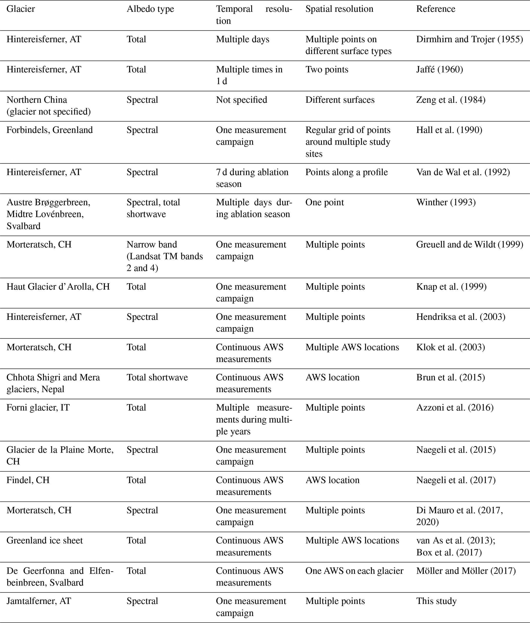
Despite the growing body of work on this topic (see Table 1), reflectance properties – spectral as well as broadband, local as well as regional, and short timescales as well as seasonal – remain understudied compared to other parameters routinely recorded at Jamtalferner and other long-term glaciological monitoring sites. However, surface changes and associated changes in the spectral characteristics in the ablation area (e.g. due to debris cover, supraglacial meltwater, deposition of impurities) are expected to play a significant role in determining the future development of these glaciers. Incorporating relevant parameters into monitoring efforts is highly desirable. The accuracy of direct measurements of mass balance depends on the representation of all surface types in the stake network and on the correct attribution of unmeasured areas to measured stake ablation. Accordingly, a better understanding of how surface types differ in terms of their reflective properties is required to maintain the stake network on a rapidly changing glacier. To this end, it is important to understand whether satellite-derived data can provide a basis for defining surface classes to be covered by stakes or whether it does not allow for the retrieval of the full bandwidth of reflectance variability relevant to the ice melt rate. In addition, delineating the temporal variability in reflectance properties is relevant to degree day modelling, as a changing albedo would alter parameters in the model.

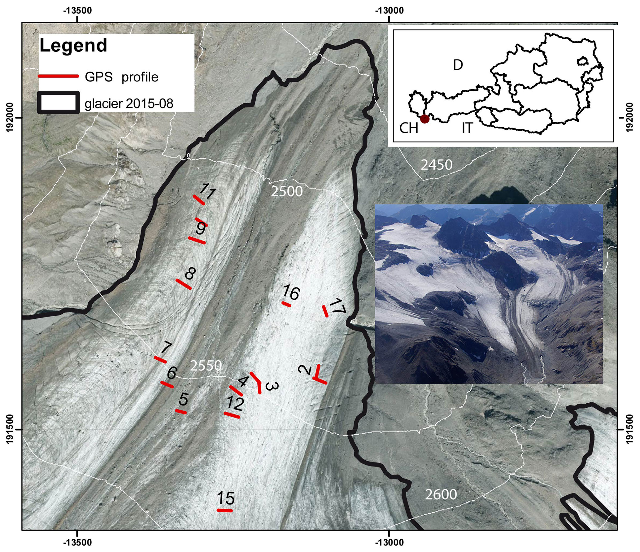
Figure 1 Glacier tongue of Jamtalferner (Orthophoto, August 2015, Source: Tyrolean Government/TIRIS) with profile lines of spectroradiometer measurements indicated in red. Insert: aerial photograph of Jamtalferner, 20 September 2018 (Photo: Andrea Fischer).

2 Data, methods, and study site

2.1 Study site – glaciological background

Jamtalferner was chosen for this study as it has the smallest end-of-season snow cover amongst the glaciers with long-term mass balance monitoring in Austria. Jamtalferner is located in the Silvretta mountain range, which intersects the border between Austria and Switzerland. Jamtalferner is the largest glacier on the Austrian side of Silvretta (Fig. 1; size in 1970 – 4.115 km², size in 2015 – 2.818 km²). The history of scientific research at the site goes back as far as 1892, when length change measurements were first carried out, and a wealth of cartographic, geodetic, and glaciological data are available (Fischer et al., 2019). Orthophotos and cartographic analysis show that debris cover at the glacier terminus and in the lower-elevation zones has increased (debris-covered percentage of total area was 1.7 % in 1970 and 24.1 % in 2015), while firn cover is decreasing (firn-covered area in 1970 was 75 %; in 2015 it was 13 %; mean accumulation area ratio – AAR – in 1990/91–1999/2000 was 0.35; mean AAR in 2010–2017/18 was 0.12; Fischer et al., 2016).

Mass balance measurements via the direct glaciological method began in 1988/89. In recent years, increasing mass loss was recorded across all elevation zones (Fischer et al., 2016). The lowest-elevation zones are dominant in terms of total ablation and thus net balance. Melt in the lowest altitudes has been increasing during the last 2 decades of negative mass balances, and the variability in surface albedo at and near the glacier terminus affects melt over the full duration of the ablation season.

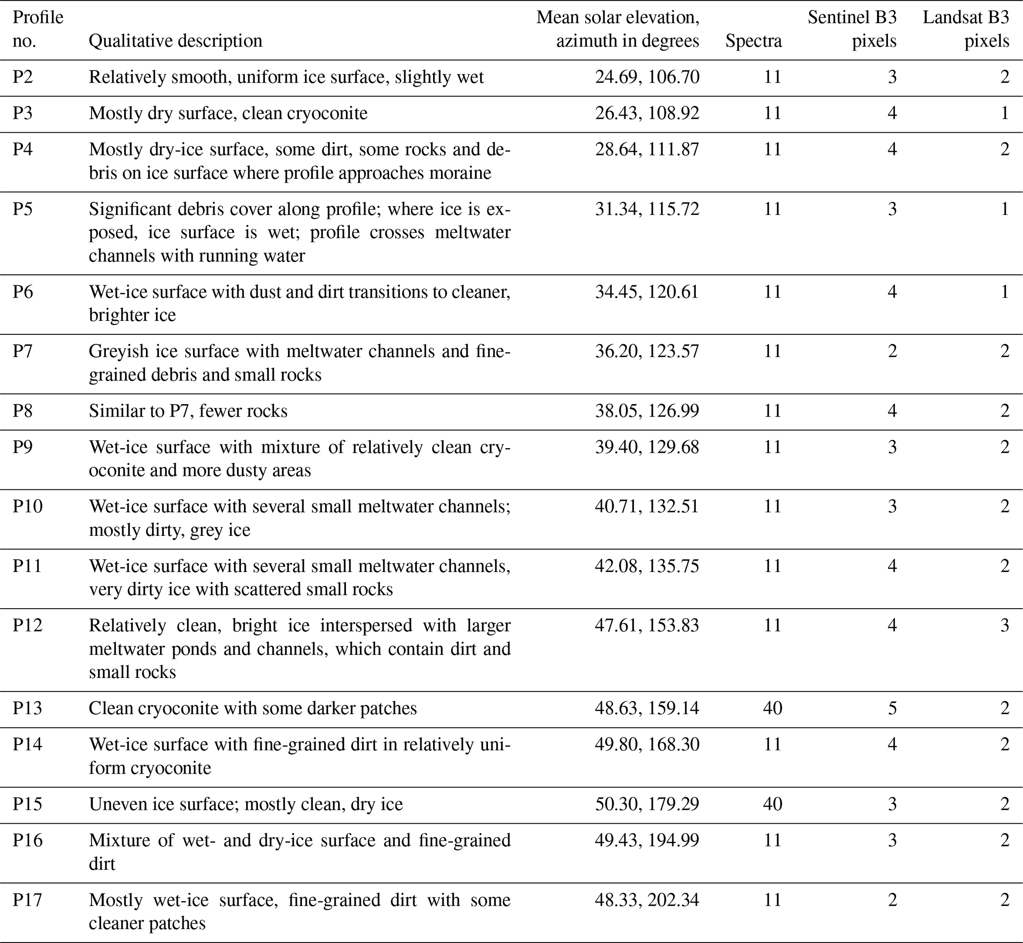
Table 2 Description of the surface characteristics along each profile line, as well as number of spectra collected along the line and number of pixels intersected by the line in band 3 (B3) of the Sentinel and Landsat scenes, respectively.

2.2 In situ measurements of spectral reflectance

The field campaign was carried out on 4 September 2019. This date was selected for two reasons: favourable weather conditions and temporal proximity to overpasses of both Sentinel-2 (on the same day) and Landsat 8 (on 3 September). With a large area of high pressure over western and central Europe, the weather at the study site was sunny and dry throughout 3 and 4 September. Using an ASD FieldSpec HandHeld 2 spectroradiometer (ASD Inc., 2020), a total of 246 reflectance spectra (HCRFs) were collected, with 12 spectra measured at point locations and 234 spectra measured along 16 profile lines. Profiles were measured along a 20 m measuring tape in such a way that individual spectra were gathered at equal intervals, with 14 profile lines containing 11 spectra spaced at 2 m. Two profiles contain 40 spectra – these were also gathered at equal intervals but with a higher resolution. Measurements began at 08:28 GMT (10:28 local time) and ended at 13:43 GMT. The coordinates of the start and end points of each profile line, as well as any spectra measured outside of the lines, were recorded with a Garmin eTrex Vista HCx, a standard handheld GPS device, which also recorded the time of day. The horizontal accuracy of the GPS coordinates is better than 3 m as per the internal accuracy assessment of the GPS device. The timestamps of the GPS points for the start and end points of the profiles were used to compute solar elevation and azimuth. For each profile, the mean solar elevation and azimuth between the respective start and end points is given in Table 2. Measurements were taken 35 cm above ground from nadir with a bare fibre-optic cable without additional fore-optics. Test measurements in the field showed high consistency between multiple measurements at the same point, so we chose to use single measurements at each location rather than an average over multiple measurements. The instrument was handheld and not mounted on a stand to minimize shading. This measurement set-up is similar to that of previous studies (Naegeli et al., 2015; Di Mauro et al., 2017) and yields a circular field of view (FOV) with a radius of approximately 7.8 cm for flat ground. The instrument operates between 325 and 1075 nm with an accuracy of ±1 nm and a resolution of < 3 nm at 700 nm. We used a feature of the instrument that allows the user to save the white-reference measurement to the RAM of the built-in computer. The HCRF is computed for subsequent target reflectance measurements based on the saved reference. This is saved to the output file, eliminating the need to calibrate the target measurements to the white reference in post-processing. A new SRT-99-020 Spectralon material (serial number 99AA08-0918-1593) manufactured by Labsphere was used for the measurement of the white reference. The ASD data files were imported into a Python script for further analysis using the Python module SpecDAL (Lee, 2017) to read the ASD format. Further data analysis was carried out using numerous other Python (Van Rossum and Drake, 2009) packages, mainly NumPy (van der Walt et al., 2011), pandas (McKinney, 2010), Matplotlib (Hunter, 2007), Rasterio (Gillies et al., 2013), GeoPandas (GeoPandas developers, 2019), rasterstats (Perry, 2015), and PyEphem (Rhodes, 2020).

Figure 2 Jamtalferner as seen in the Sentinel (a) and Landsat (b) scenes used in this study. The images shown here are composites of bands 2, 3, and 4 of each satellite's L2A surface reflectance product displayed at a resolution of 10 and 30 m (Sentinel and Landsat, respectively) per pixel. Profiles where reflectance spectra were collected are marked in red. Coordinate reference system – EPSG:32632.

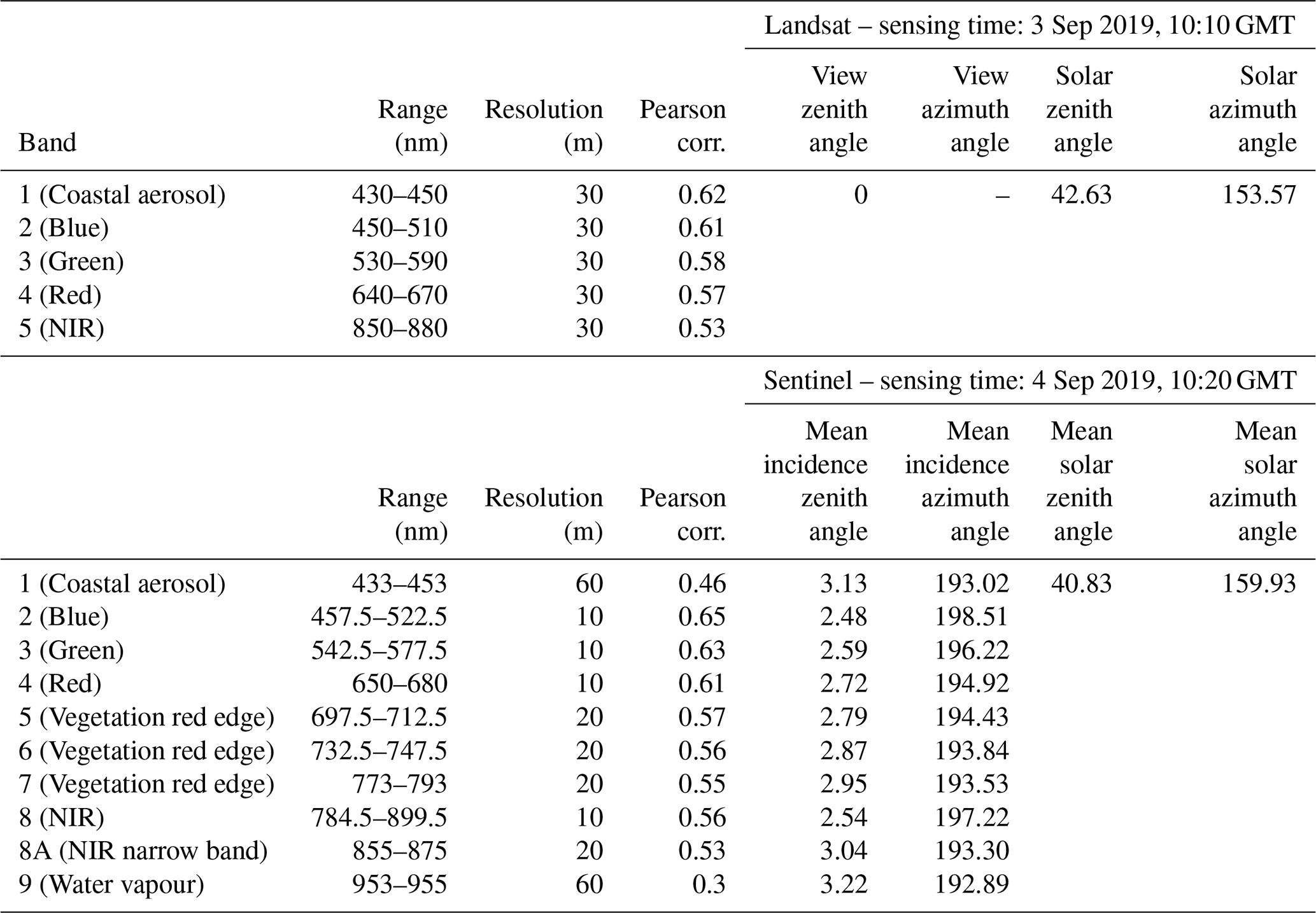
Table 3 Band names and respective wavelength range and resolution for Landsat and Sentinel as used in this study. Pearson correlation given for mean band values of ground measurements and associated satellite data. For Landsat, the solar zenith and azimuth angles given in the surface reflectance image are listed. The view zenith angle is hardcoded to 0 in the Land Surface Reflectance Code (LaSRC_1.3.0) for the Landsat surface reflectance product, as per the LaSRC documentation (USGS, 2020). For Sentinel, the incidence angles refer to the mean viewing zenith and azimuth angles for each band. The solar angles are the averages for all bands.

2.3 Satellite data

We compare the in situ measurements with surface reflectance products derived from a Landsat 8 Operational Land Imager (OLI) scene acquired on 3 September 2019 (10:10 GMT), the day before the field campaign, and a Sentinel-2A scene acquired on 4 September (10:20 GMT), the same day as the field campaign. Both scenes are cloud-free over the study area (Fig. 2). Details on the atmospheric-correction algorithm used to generate the Landsat 8 OLI level-2 surface reflectance data product from top-of-atmosphere (TOA) reflectance can be found in Vermote et al. (2016) and in the product guide of the algorithm used to derive surface reflectance (USGS, 2020). Details on the equivalent Sentinel-2 product – the level-2A bottom-of-atmosphere reflectance – are given in Main-Knorn et al. (2017) and Richter and Schläpfer (2011). For the sake of readability, we refer to the Landsat 8 OLI level-2 surface reflectance as “Landsat” data in the following, and to the Sentinel-2 level-2A surface reflectance as “Sentinel” data. The Landsat and Sentinel surface reflectance raster data used in this study were acquired using Google Earth Engine (Gorelick et al., 2017).

The wavelength range of the spectroradiometric measurements carried out on the ground overlaps with bands 1–5 of the Landsat data and bands 1–9 and 8A of the Sentinel data, respectively. Only spectral ranges covered by these bands are considered for this study. The wavelengths and resolution of the individual bands, as well as the relevant viewing and solar angles, are given in Table 3. For each ground measurement point, band values were extracted from the satellite scenes at the overlaying pixel.

In order to compare the satellite values with ground data, we compute mean values for the subsets of the spectral reflectance curves measured on the ground that correspond to the Landsat and Sentinel bands, respectively. Data are then grouped into profile lines and/or different bands; the Pearson correlation is computed for ground data and corresponding satellite data, and further comparisons are carried out using standard statistical metrics.

To assess the influence of the spatial resolution of the satellite data on results, band-3 imagery was resampled (cubic interpolation) from the original 10 m resolution to 30 and 60 m for Sentinel and from 30 to 60 m for Landsat. To account for the potential effects of the uncertainty in the GPS coordinates, we created a circular buffer with a radius of 3 m around each in situ measurement point. For each buffer, the corresponding satellite value is computed as the median of the values of all pixels the buffer overlaps with.

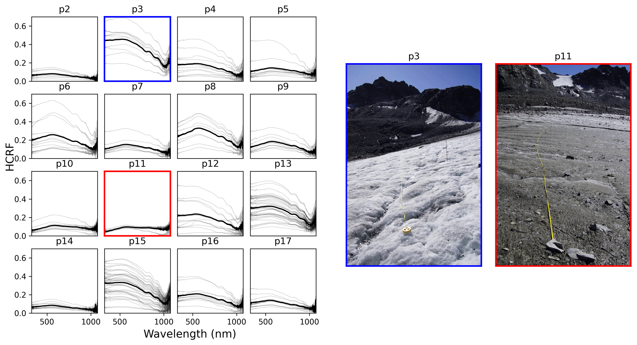
Figure 3 Each subplot on the left shows the spectra along a profile line. The bold black lines highlight the mean spectral reflectance (HCRF) in each profile. Photos of the ice surface along p3 and p11 are shown on the right for visual context. Photos were taken at the time of the respective measurements by Andrea Fischer.

3 Results

3.1 Surface measurements

The in situ measurements exhibit extreme differences in HCRFs depending on the characteristics of the surface. Figure 3 shows the spectra grouped into profiles, with the mean spectral HCRF highlighted for each profile. P3 is the “brightest” profile, with the highest maximum (up to 0.7) and minimum (up to 0.2) values of all profiles. Profiles 2, 11, and 14 are the darkest profiles, and all of their respective spectral reflectances remain below 0.2 at all measured wavelengths. Figure 3 also shows the ice surface along profile lines 3 (brightest) and 11 (darkest) for a visual comparison. In P3, the surface mainly comprises clean, dry ice. In P11, the ice surface is wet and impurities (rocks, fine-grained debris) are present. The profile line crosses several small meltwater channels with running water.

Table 2 contains a qualitative description of the ice surface along each profile line, the length of the line, the number of spectra per line, and the number of Landsat and Sentinel band-3 pixels that each line crosses, as well as the mean solar elevation and azimuth angles for the profile. The maximum number of pixels per line is 5 for Sentinel and 3 for Landsat. All lines cross at least 2 pixels for Sentinel, while three lines fall into a single Landsat pixel. See Fig. 1 for the location of each profile on the glacier.

The spectral reflectance curves of the individual spectra as well as of the profile lines indicate high spatial variation in surface types and associated reflective properties. The spectral signatures of the individual spectra can roughly be grouped into dry ice, wet ice, and dirt or rocks. (We use the word “dirt” to describe all types of mineral or organic materials and fine-grained debris that may collect on the glacier surface.) However, transitions between these types are gradational, and in practice these categories cannot always be clearly separated – both dry and wet ice might be clean or dirty; dirt might be wet or dry.

The reflectance curves for clean ice exhibit the typical shape frequently found in the literature (Zeng et al., 1984), with the highest reflectance values (up to 0.69) in the lower third of our wavelength range and declining values for wavelengths greater than approximately 580 nm. The spectral reflectance curves of wet-ice surfaces follow roughly the same shape as for dry ice but are strongly dampened in amplitude with reflectance values typically not exceeding 0.2. In contrast, the reflectance curve of dirty surfaces remains at uniformly low values throughout our wavelength range in some cases and exhibits an increase of between 325 and approximately 550 nm before flattening out in other cases. Reflectance values have similar magnitudes to those for wet ice. Example reflectance curves of these surface types are given in Fig. 4.

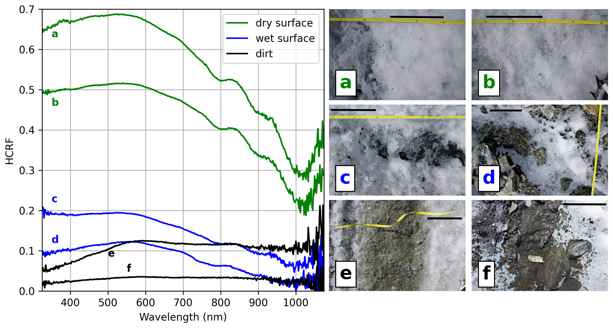
Figure 4 Spectra of different kinds of ice surface types encountered in the ablation zone of Jamtalferner. The photos on the right show the ice surface at the sampling sites of the respective spectra. The black bar in each photo represents approximately 20 cm, to provide a sense of scale. The spectra shown in this figure are part of the following profile lines: (a–c) p3, (d) p4, (e) p6, and (f) p12.

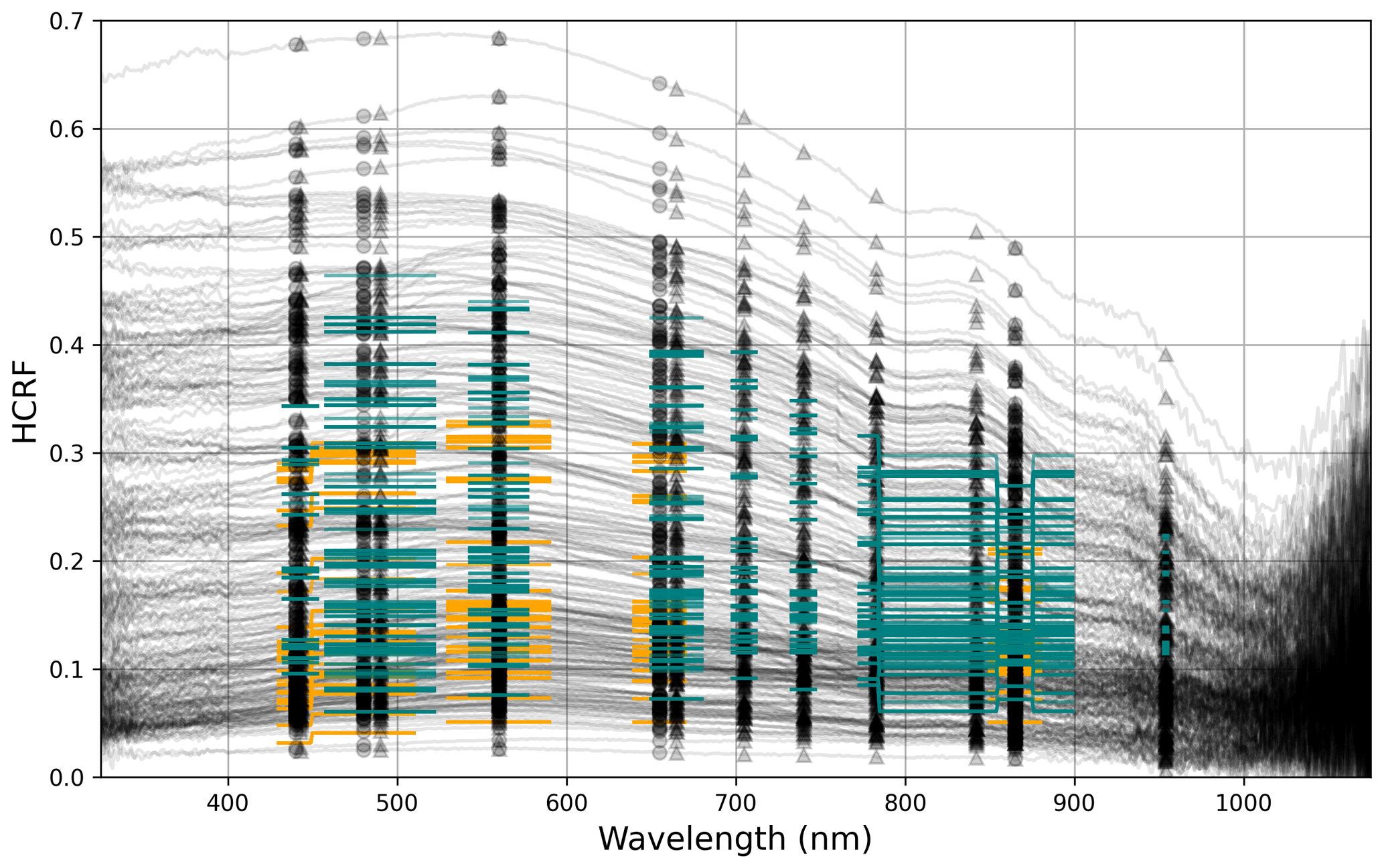
Figure 5 The spectra measured in situ are plotted in black. Black circles indicate the central wavelengths of the Landsat bands; black triangles indicate those of the Sentinel bands (see Table 3). Orange and teal lines represent the wavelength range of the respective Landsat and Sentinel bands along the horizontal axis and the satellite-derived reflectance at the sampling points of each spectrum on the vertical axis.

3.2 Comparison with satellite data

Figure 5 shows all measured spectral reflectance curves, as well as the Sentinel and Landsat values in the bands that overlap the wavelength range of the ground measurements. Reflectance values were extracted from the satellite imagery at the coordinates of each sampling point and overlaid onto the plots of the in situ spectra as coloured bars. Naturally, neither satellite captures the full range of reflectance values measured on the ground. In all overlapping bands of Sentinel and Landsat, the Sentinel values are higher, in the sense that the maximum values of the Sentinel data are closer to the maximum values measured on the ground, while the minimum Landsat data are closer to the minimum values measured on the ground.

Comparing the mean of the HCRF spectra measured on the ground for each satellite band with the associated satellite values yields a Pearson correlation coefficient ranging from 0.53 (band 5) to 0.62 (band 1) for the Landsat bands and 0.3 (band 9) to 0.65 (band 2) for Sentinel. Table 3 lists the correlation coefficients, as well as the wavelength range and resolution of each band. The two lower-resolution Sentinel bands (band 1, band 9 – 60 m resolution) have notably lower correlation coefficients than the higher-resolution bands. The Sentinel and Landsat data at the in situ measurement points are strongly correlated with each other in the bands where both satellites overlap, with r=0.69 in band 1 and r>0.8 for bands 2, 3, 4, and 5.

For a visual comparison of the location of the profile lines and the range of measured values in the profiles in relation to the satellite pixel boundaries and pixel band values, see Fig. 6 for Sentinel (band 3 selected as an example) and the Supplement for an analogous figure of the Landsat data.

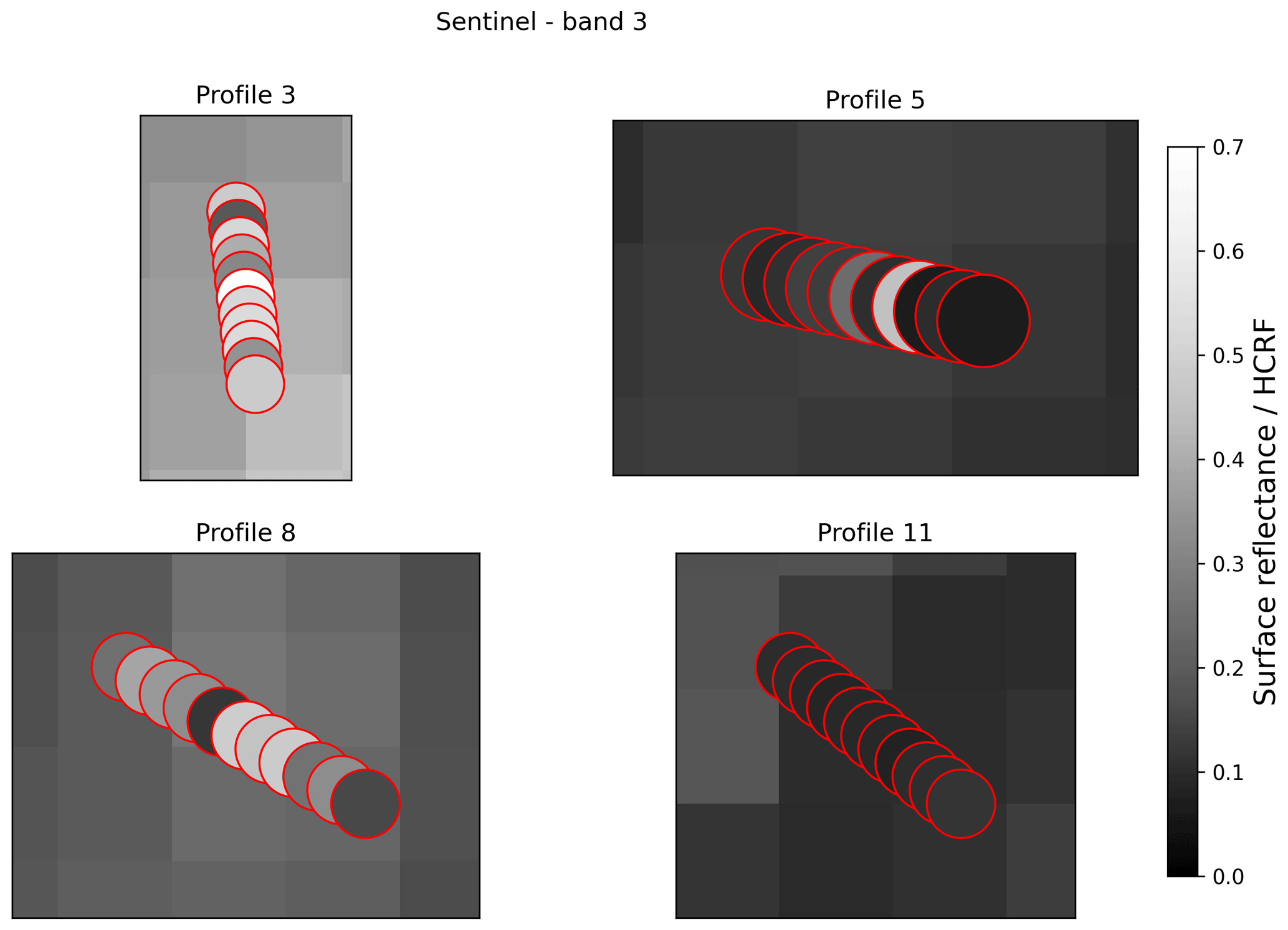
Figure 6 The spectra comprising the profile lines are plotted over the corresponding satellite pixels for selected profiles. The colour bar is the same for the background raster and the circles indicating the sampling sites of the spectra and represents the Sentinel band-3 pixel value and the mean reflectance in the Sentinel band-3 wavelength range of each spectrum, respectively. The pixel size of the raster is 10 m². The GPS coordinates of the sampling sites are centred in the circles. The circle radius is set to 3 m to represent the horizontal uncertainty in the GPS points.

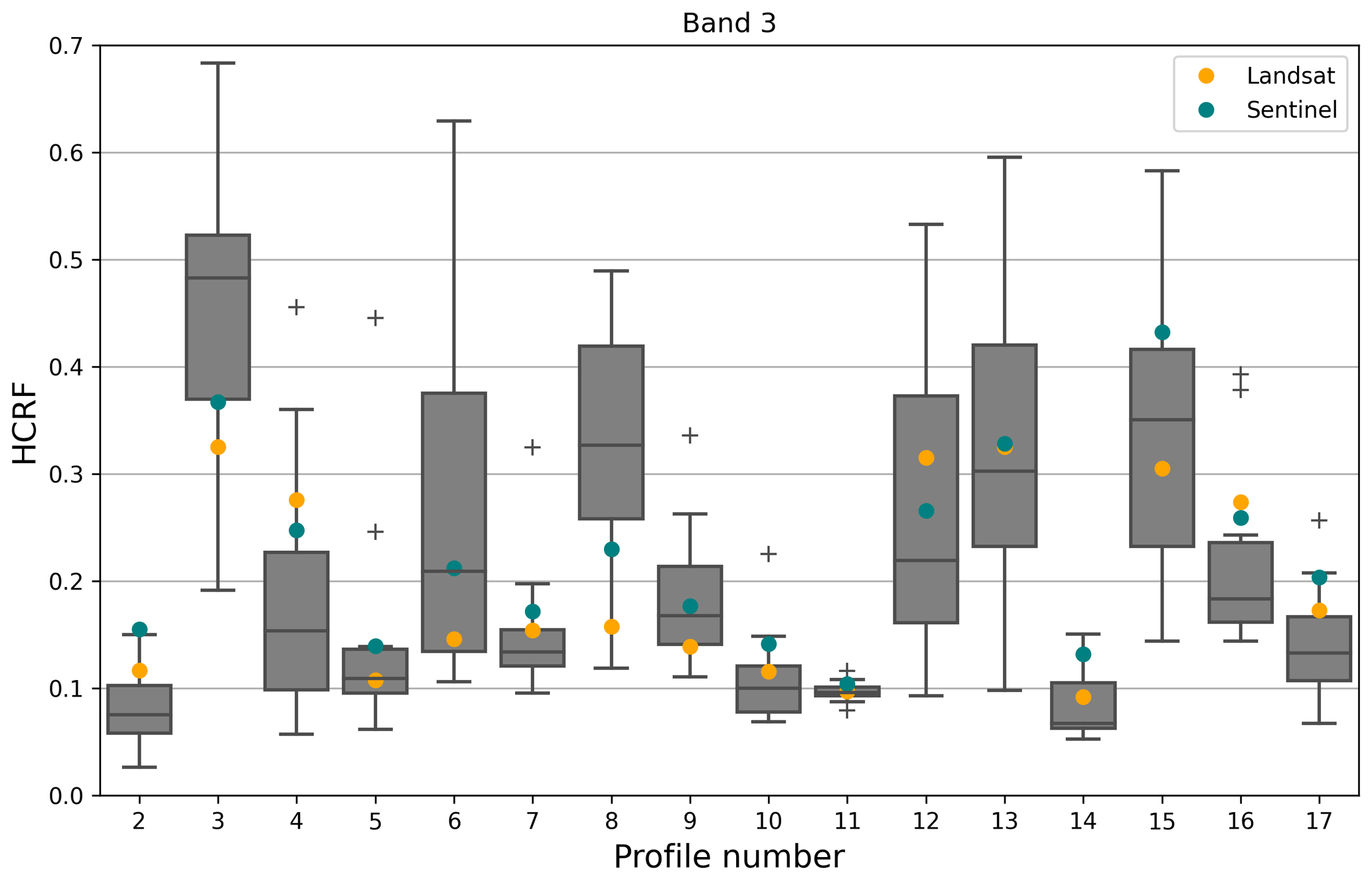
Figure 7 Spread of the Sentinel band-3 (wavelength range: 542.5–577.5 nm) mean values of the measured spectra, grouped by profile. Orange and teal circles show corresponding mean pixel values of data extracted from Landsat and Sentinel pixels at the sampling sites of the spectra, respectively. The boxes represent the first and third quartile. The whiskers represent 1.5× the interquartile range; the + symbols are outliers.

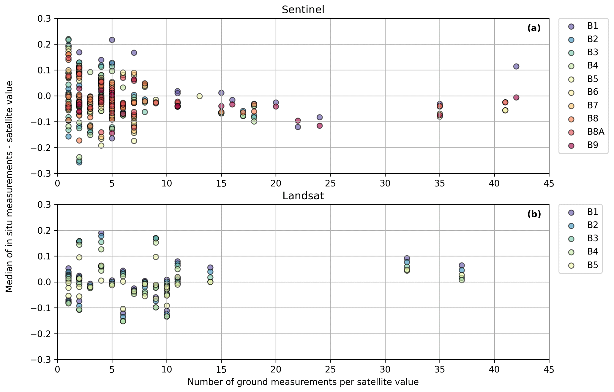
Figure 8 The number of ground measurements per unique satellite value (x axis) is plotted against the difference between the median of these ground measurements in the respective wavelength band and the corresponding satellite value (y axis); i.e. values that are positive in the vertical axis represent cases where ground reflectance is higher than satellite-derived reflectance, whereas negative values represent the opposite. Different colours represent the different satellite bands, as indicated by the legends next to the plots.

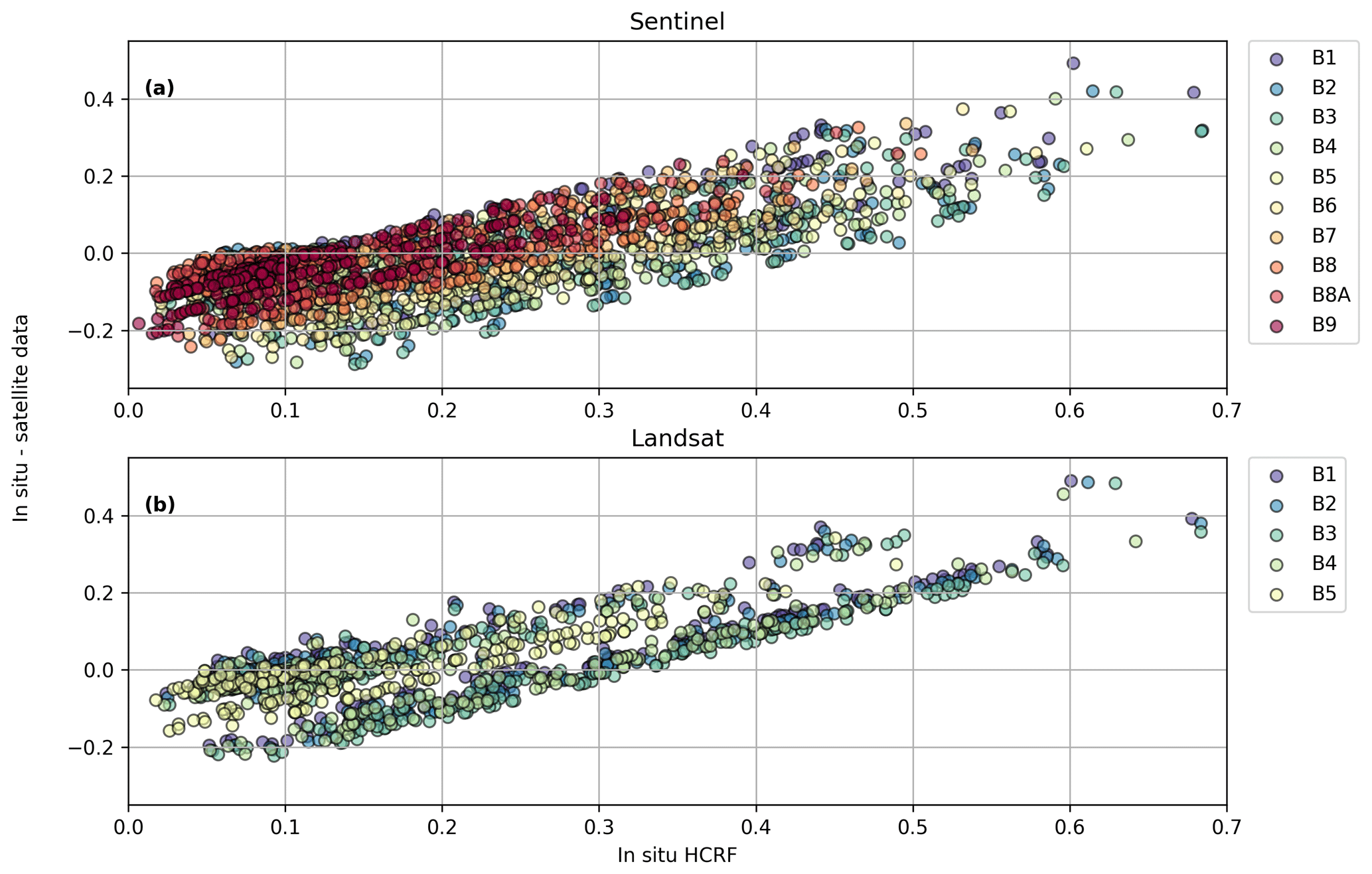
Figure 9 Same data as in Fig. 8 but showing individual sampling points without grouping by common satellite pixels.

The spread of in situ HCRF values per profile is generally lower for profiles that are darker overall and greater for brighter profiles, although not in all cases (Figs. 3, 7). In the Sentinel band-3 wavelength range, profile 3 is brightest with a median reflectance of 0.48 and spread of 0.49. Profile 6 (median in Sentinel band-3 range is 0.21) has the largest spread of HCRFs (0.52). Broadly speaking, profiles with a high median HCRF tend to include individual measurement points that are both very bright and very dark, while darker profiles are more uniformly dark. Profile 6 in particular transitions between surface types and contains wet and dirty spectra as well as dry-ice spectra (see Table 2). Figure 7 shows boxplots of the ground measurements (band-3 mean) for all profiles to exemplify this and indicates where the Landsat and Sentinel values fall compared to the spread of values in each profile.

When binning in situ measurements by the associated satellite value or pixel and taking the median or mean of the binned values, the difference between the median or mean in situ value and the satellite value tends to decrease with an increasing number of in situ measurements mapped to unique satellite values. This is to be expected, as each satellite value represents an integration of the emission characteristics over the area contained in the pixel. However, for our data, this relationship is not obviously linear and differs between Sentinel and Landsat, as well as between different bands (Fig. 8).

Comparing in situ and satellite values for individual in situ measurement points, it is apparent that both satellites tend to overestimate the reflectance values of dark ground surfaces and underestimate the reflectance of bright surfaces, in all bands (Fig. 9). The shift from over- to underestimation appears linear and has a similar increase rate in all bands. The zero crossings of the regression lines, i.e. the ground reflectance values for which ground measurements and satellite values match, fall between 0.15 (band 5) and 0.21 (band 1) for Landsat and 0.17 (band 9) and 0.27 (band 3) for Sentinel.

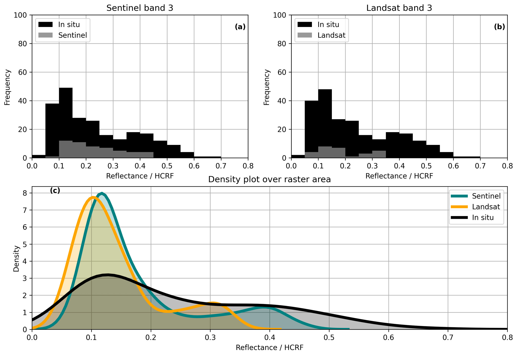
Figure 10 The histograms in panels (a, b) show the frequency of occurrence of the band-3 mean values of the ground measurements per reflectance bin. Bin width: 0.05. Overlaid in grey are the histograms of the corresponding satellite pixel values. Panel (c) shows density plots of the Sentinel and Landsat band-3 surface reflectance rasters over the study area (smallest possible rectangle containing all ground measurements), with the density of the in situ HCRFs for comparison.

Figure 10 shows histograms of the mean reflectance in band 3 of Landsat and Sentinel, respectively, compared with associated in situ values, as well as density plots of the satellite-derived surface reflectance over all pixels in the study area. The mean is highest in the in situ measurements and lowest in Landsat images. Both Sentinel and Landsat fail to capture HCRF values below 0.05 and above 0.45. A second peak in frequency evident from the in situ measurements at a reflectance of 0.4 is not represented in the remote sensing data.

Table 4 Comparison of in situ and satellite data by the standard deviation (SD) of the difference between in situ HCRF and satellite surface reflectance. Values are grouped by number of pixels that buffered in situ measurements overlap.

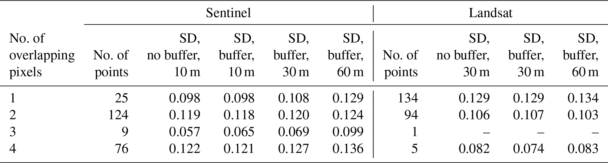
To conclude the results, a note on the sensitivity of data and results to the spatial resolution of the satellite data and the accuracy of the geolocation of the in situ data follows: to assess the possible effects of the GPS accuracy or lack thereof, we compare the differences between in situ and satellite values presented previously to the differences that result when a buffer corresponding to the GPS uncertainty is created around each in situ measurement point. For the Sentinel data in the original 10 m resolution of band 3, the maximum number of pixels that any buffer touches is 4, the mean is 2.6, and most buffered in situ measurement points overlap with 2 pixels. For the 30 m Landsat data in band 3, the maximum number of pixels touched is also 4, the mean is 1.5, and most in situ points are fully within only 1 pixel. Table 4 gives the standard deviation of differences between the in situ HCRF and the satellite data in different resolutions, grouped by the number of pixels the buffered measurement points overlap with, to show how variability in results shifts depending on the buffer and the raster resolution. Changes caused by introducing the buffer are small in all groups. As expected, standard deviation increases with decreasing resolution of the satellite pixels due to the loss of detail in the satellite data. Figure 11 gives an overview of the ungrouped data set with and without the buffer and at different raster resolutions.

4 Discussion

There are a number of complexities associated both with measuring reflectance properties on the ground and with any comparison between different products and data sets. Perhaps more than anything else, our results highlight the need for further in situ measurements and targeted data collection campaigns designed specifically to address some of the uncertainties detailed in the following.

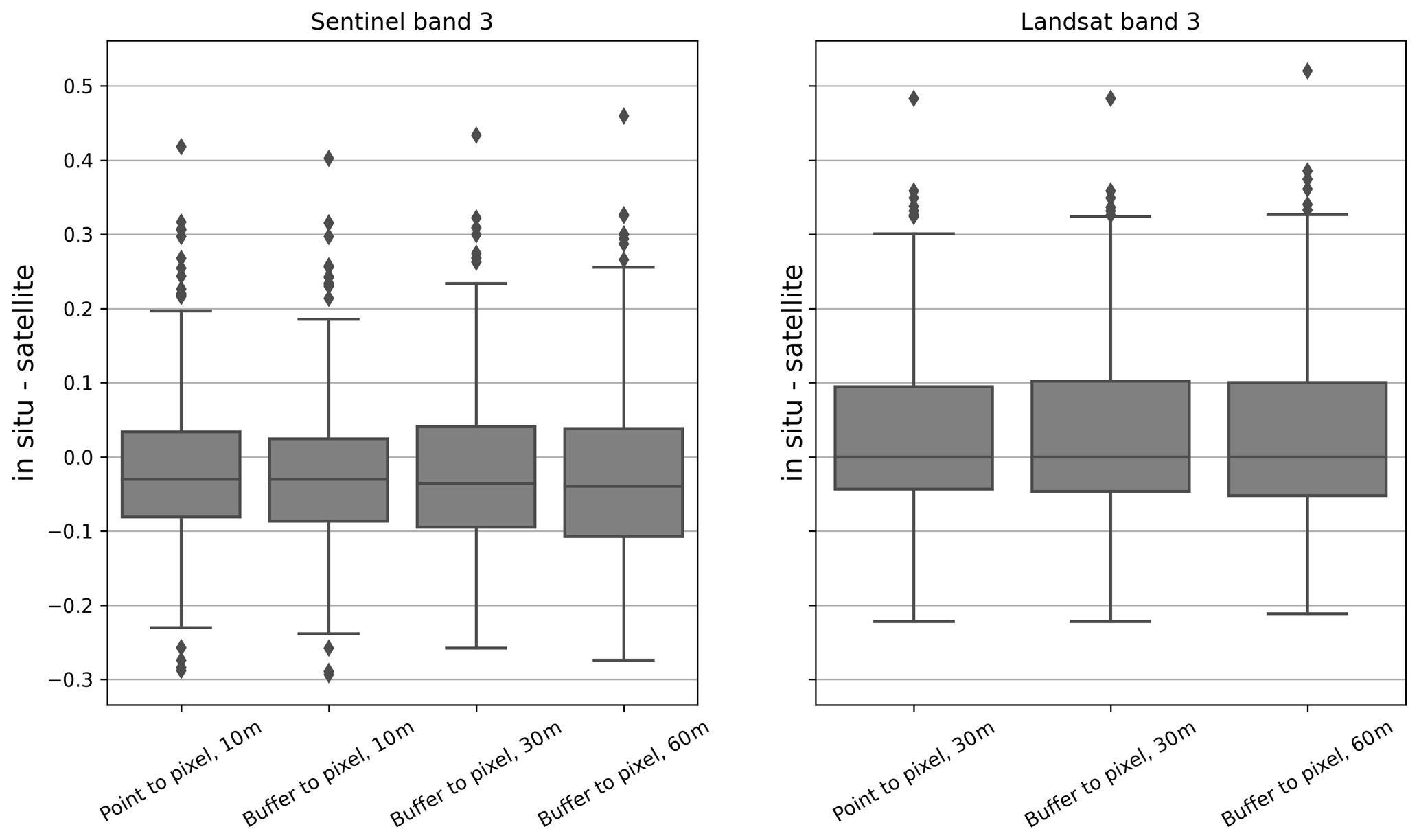
Figure 11 For the respective Sentinel and Landsat band-3 wavelength range, the difference between the in situ HCRF and satellite surface reflectance product is on the vertical axis. Point to pixel refers to the data as presented in previous figures. Buffer to pixel refers to data generated using a buffer around the in situ measurement points to account for GPS accuracy. For Sentinel, the original 10 m resolution data were resampled to 30 and 60 m. For Landsat, the original 30 m resolution data were resampled to 60 m.

4.1 Reflectance anisotropy and changing solar and atmospheric conditions

Ice is an anisotropic material, and previous studies have shown that for glacier surfaces, anisotropy increases with decreasing albedo and depends on wavelength and solar zenith angle (Greuell and de Wildt, 1999; Klok et al., 2003; Naegeli et al., 2015). In order to truly quantify the effects of anisotropy in in situ spectroradiometric measurements, the bidirectional reflectance distribution function (BRDF) must be obtained – ideally for each measurement point. The BRDF cannot be measured directly but is approximated, e.g. by interpolating between multi-angular spectroradiometer measurements (Naegeli et al., 2015) or with modelling approaches (Malinka et al., 2016). While multi-angular HCRF measurements allow for the estimation of the BRDF, they are intrinsically dependent on the atmospheric conditions (cloud cover) at any given time, as well as on the topography and structure of the surface. Naegeli et al. (2015, 2017) use this approach to develop anisotropy correction factors for different glacier surface types in order to account for the typical underestimation of albedo in observations from nadir in remote sensing data. They find a difference between corrected and uncorrected albedo values of up to 11 % for dirty ice in airborne imaging spectroscopy data. Nonetheless, the application of constant correction factors for clustered surface types is a simplification that obscures both the gradational nature of surface classification and the complexity of accounting for the effects of varying surface roughness on effective illumination angles. We consider a quantitative assessment of anisotropy beyond the scope of our study and hope to tackle this issue in detail in future work. We assume that our in situ data as well as the satellite products underestimate the quantities they measure (HCRF and surface reflectance as per the respective documentation of the satellite products) due to the nadir or near-nadir observational angle, in particular for dark surfaces, and that uncertainties caused by anisotropy are likely to be in the range found by Naegeli et al. (2017). The local variability in reflectance properties of glacier ice comprises the spectral, as well as spatial and temporal, variability in reflectance anisotropy, which requires a combination of targeted, continuous measurements and modelling that accounts for the surface roughness of different glacier surface types to truly delineate.

The weather on 3 September (Landsat overpass) and 4 September (Sentinel overpass, in situ measurements) 2019 was very favourable. There was no cloud cover at the study site during either of the satellite overpasses and for the duration of the field measurements, and we consider any changes in atmospheric conditions to be negligible. While the illumination angles naturally change over the course of the day and accordingly changed during the in situ measurements (Table 2), very low solar elevation angles were avoided. In their study on parametrizing BRDFs for glacier ice and Landsat TM, Greuell and de Wildt (1999) show that the spectrally integrated albedo of dark ice changes with the solar zenith angle and is particularly low for low zenith angles. Accordingly, we acknowledge that the changing solar angles are a source of uncertainty in our data and in the comparison with the satellite-derived reflectances, but we consider this uncertainty relatively small since measurements were carried out within the few hours before and after the satellite overpasses, avoiding very low solar elevation angles. Greuell and de Wildt (1999) also point out that the drop in albedo for low zenith angles is related to the presence of meltwater at later times of day (lower zenith angles), which highlights the difficulty of isolating one variable (zenith angle) in a complex system with multiple variables that change over time (surface processes like meltwater affecting reflectance properties).

The Landsat and Sentinel surface reflectance products both incorporate an atmospheric correction applied to TOA reflectance in the generation of the BOA product (Vermote et al., 2016; Main-Knorn et al., 2017). This introduces some uncertainty into the comparison with in situ data since the correction methods differ. Nonetheless, we believe that assessing how in situ data compare to the frequently used surface reflectance products of the Landsat 8 and Sentinel-2 suites is a necessary first step in being able to determine whether custom atmospheric corrections would improve results and if such improvements would be large enough to outweigh the added complexity and computational cost. We suggest that the answer to this question depends on the application and the spatial scale of the intended analysis. Again, this is beyond the scope of the presented study and is a point that needs to be specifically addressed in future work. We suggest that case studies at individual, well-studied glaciers can serve as an ideal testing ground for such issues and will help to determine whether custom atmospheric corrections should be applied and are feasible on a regional or even global scale in satellite-based studies of ablation area reflectance properties.

4.2 Implications of in situ and satellite comparison

The results presented in Sect. 3.1 highlight the large spatial variability in HCRF and different surface types encountered in the ablation area, both of which are in line with findings from other studies (Naegeli et al., 2015, 2017; Di Mauro et al., 2017). Section 3.2, the comparison of the in situ data with satellite values, arguably presents greater challenges in terms of interpretation and implications of the results.

In summary, there are three key findings which we believe may be important for further studies and for delineating the relationship between in situ and satellite-derived reflectance:

• Sentinel surface reflectance values tend to be closer to the higher end of HCRF values measured in situ, while Landsat tends to be closer to the in situ minimum.

• The difference between in situ data and satellite data tends to decrease when there are more in situ data points per pixel but not always and not in a clearly linear way.

• The reflectance of dark surfaces tends to be overestimated in the satellite products, while the reflectance of bright surfaces tends to be underestimated.

Explaining the above points in full requires targeted investigations specifically addressing the contributing factors and uncertainties, which – with our current data set – we can only provide a qualitative overview of.

As mentioned previously, different atmospheric corrections are used for the Sentinel and Landsat surface reflectance products. This may contribute to systematic differences in how surface reflectance is represented under differing lighting conditions and in different spectral ranges. Efforts to harmonize the Landsat and Sentinel surface reflectance data sets have great potential for minimizing this problem for applications where data from both satellites are used (Claverie et al., 2018).

Another issue that deserves more detailed attention is the narrow and spectral to broadband conversion required for comparing satellite reflectance in individual bands with the in situ data of the same wavelength range. We intentionally do not compute a shortwave broadband albedo from the satellite band values or the spectral in situ data to avoid introducing a further source of uncertainty. Instead, we limit ourselves to averaging over the band wavelength range in order to keep the comparison as straightforward as possible, but we acknowledge that a glacier-wide broadband albedo is a key parameter for many regional or global modelling applications.

The standard atmospherically corrected BOA reflectance products from satellite data are provided without correcting for the BRDF. The BRDF, describing the change of the reflectance with different observation and incidence geometries, can have a significant impact on the satellite-based reflectance as well as on the in situ data, leading to inherent challenges when comparing satellite-based BOA reflectance with in situ reflectance measurements (Schaepman-Strub et al., 2006). Correcting Landsat and Sentinel surface reflectance with MODIS or VIIRS (Visible Infrared Imaging Radiometer Suite) BRDF products to produce surface albedo has been shown to be a viable approach in some cases (Shuai et al., 2011; Li et al., 2018), but the coarse resolution of MODIS and VIIRS data is unlikely to capture the small-scale anisotropy effects of different glacier surface types. This would therefore be of limited use for our purposes. Optimizing methods for computing surface albedo from the level-2A (L2A) products, as well as from the in situ HCRF, requires further study and customized solutions accounting for local topographic effects and the spectral characteristics of the surfaces. We assume that for our case uncertainties due to the intrinsic difference between the HCRF and the satellite-derived HDRF (hemispherical–directional reflectance factor) are small compared to other sources of uncertainty: the influence of local topography as a source of indirect radiation is not represented in the satellite-derived values, and the microstructure of the ice surface may locally affect in situ values on a scale that is not visible to the satellite but could be very significant for in situ measurements (e.g. small ice ridges or similar features acting as reflectors and/or scattering light into the FOV of the instrument).

Hendricks et al. (2003) state for spectroradiometric measurements at Hintereisferner compared to Landsat ETM+ imagery acquired about 2 weeks before the field measurements, “The reflectance of ice seems to be highly variable with both under- and overestimations of up to 76 % and 31 %, respectively.” This corresponds well with our finding that both under- and overestimation occur frequently for both satellites. The factors mentioned above may partly explain the location of the shift from under- to overestimation (Fig. 9), but – again – targeted measurement campaigns are needed to truly quantify this.

The influence of very local backscattering could play a role in the seeming inconsistencies in the dependency of the difference between in situ and satellite data on the number of in situ measurement points per pixel (Fig. 8), but this also ties in with questions regarding the positional accuracy of the in situ measurement points and the satellite data and the spatial representativity of point measurements for a larger area.

Our comparison of in situ and satellite data is based on the assumption that we know where both are located in a common coordinate reference system to a sufficient degree of accuracy. The accuracy of the position of the GPS points at the start and end points of the measurement profiles is approximately 3 m. Sentinel-2 orthorectification is based on the PlanetDEM 90 digital elevation model (DEM), which incorporates the SRTM (Shuttle Radar Topography Mission) DEM in areas where SRTM is available, such as Austria (Kääb et al., 2016). The geometric accuracy of the Sentinel data hence depends on the accuracy of the underlying DEM, which is subject to a number of uncertainties particularly over mountainous terrain. Vertical inaccuracies – which propagate into horizontal inaccuracies - increase over glacier surfaces, especially in areas with large changes in surface elevation, as the DEM can only provide a snapshot of conditions for a moment in time and quickly becomes outdated in rapidly changing environments. Pandžic et al. (2016) determine an average offset in the Sentinel-2 data for Austria of about 6 m compared to a high-resolution regional DEM. The performance requirement of Landsat 8 OLI for geometric terrain-corrected accuracy is specified as 12 m (Storey et al., 2014). Kääb et al. (2016) find cross-track offsets of 20–30 m over glacier termini in the Swiss Alps when comparing Landsat 8 and Sentinel-2 scenes acquired on 8 September 2015. Accordingly, uncertainties regarding the GPS points of the in situ measurements as delineated in our sensitivity analysis (Table 4, Fig. 11) can be considered relatively small compared to those related to the orthorectification of the satellite data. Comparisons between in situ point data and pixel values from the satellite products must be interpreted keeping positional uncertainties in mind.

Decreasing the pixel resolution and averaging over multiple in situ measurement points can serve as an approach to reduce the influence of geometric errors. However, any sort of averaging procedure must also be assessed in terms of spatial representativeness of the point measurements for a greater area and, conversely, the downsampled satellite data for small-scale surface processes. What can be considered representative will always be a question of scale and application. The glacier surface at the study site is locally very heterogenous and hence prone to representativeness errors (Wu et al., 2019). We selected the location of the in situ profile lines so that they cover what we consider to be the typical surface features and types of a given section of the ablation zone and argue that our 20 m long profile lines with equidistant measurements at least every 2 m capture any variations that are likely to influence the corresponding pixel values of the satellite data. Naturally, the less overlap there is between the profile lines and any given satellite pixel, the more likely it is that the in situ point data happen to capture something that differs strongly from what the satellite sees.

The different surface types identified at Jamtalferner (Fig. 4) and their reflectance spectra are comparable to types of surfaces identified in Switzerland at Morteratsch and Glacier de la Plaine Morte by Di Mauro et al. (2017) and Naegeli et al. (2015), respectively, supporting the use of a classification scheme based on differentiating between (a) clean- and dirty-ice surfaces and (b) the presence or absence of liquid water on the ice surface. Classifying the surface characteristics into discrete types can help to ensure representativeness, e.g. by quantifying how much of a given area subsection relevant to the comparison with remote sensing data comprises which type and then sampling accordingly. However, surface types are not always discrete in practice. Nicholson and Benn (2006) indicate that the surface albedo of ice with scattered debris can be simulated in a modelling approach by linearly varying between clean-ice albedo values and values for debris, but this does not necessarily account for other types of surfaces and even the clean-ice albedo can vary considerably, especially if liquid water is present. Additionally, classification by types of any kind cannot address the issue of temporal representativeness unless the temporal variability in different surface types is first determined.

Profile 8 shows particularly poor agreement with the corresponding satellite data and may be an example where temporal variability plays a role: the profile crosses a section of ice where the contrast between dark and bright areas is comparatively strong. The profile line is roughly at a right angle to the flow direction of the glacier, and “stripes” of meltwater channels and/or dirt cross the line. The profile has a comparable number of individual spectra with reflectance values above and below the profile mean; i.e. it is not a dark profile with a few bright outliers (compare e.g. to P6 in Fig. 6) or vice versa (e.g. P3), but the values alternate along the profile line. Agreement with the remote sensing data is decent for the darker spectra in P8, but the bright values are not captured. While we cannot rule out that the lack of agreement between the field and remote sensing data is due to an unusually unfortunate or unrepresentative positioning of the field measurement points in the satellite pixels, this may be an instance where the diurnal melt cycle and the associated presence or absence of water on the surface exacerbates the contrast between the dark and bright sections of the profile. In the bright sections, the porous weathering crust and cryoconite hole structures appear to be drained of water, while the depressions of the melt channels are noticeably wet. Cook et al. (2016) indicate the occurrence of “sudden drainage events” in the weathering crust on a day-to-day timescale and a diurnal cycle of the hydrology of the weathering crust driven by meteorological conditions (radiation, turbulent fluxes). The time of day of a satellite overpass would determine which stage of this cycle the satellite sees and consequently the satellite data would not capture this variability. In order to assess how much the time of day of the overpass could systematically affect the representativeness of the satellite date for actual ground reflectance, it needs to be determined how significant and how consistent the diurnal cycle is. To do this, the driving processes must be identified, keeping in mind that these may be different for different types of glaciers and that different causes of short-term albedo change can overlap. For example, Azzoni et al. (2016) point out that meltwater increases albedo around midday in a daily cycle, while rain causes increased albedo for up to 4 d after the precipitation event. A seasonal cycle of albedo has been demonstrated in previous observational studies and modelling efforts of broadband albedo, highlighting the importance of continuous measurements (e.g. Hoinkes and Wendler, 1968; Nicholson and Benn, 2013; Möller and Möller, 2017).

4.3 Relevance of small-scale variability

The reflectance properties of ice are a central part of mass and energy balance modelling, usually in the form of a glacier-wide broadband albedo or using one value for ice in the ablation zone and one for snow-covered areas. Resolving local albedo variations at a very small, subpixel scale is not required for regional or global studies, provided the albedo parametrization captures the conditions on the ground adequately for the region of interest. In their important 2015 study, Naegeli et al. find that Sentinel-2 and Landsat 8 reflectance data are within the suggested accuracy requirements for global climate modelling (±0.05; Henderson-Sellers and Wilson, 1983) over their study site, Glacier de la Plaine Morte in Switzerland. In the same study, they report a 10 % difference in modelled mass balance when a spatially distributed albedo is used to force the model as opposed to a single, glacier-wide albedo. Significantly larger differences occur in parts of the glacier where water is present on the surface or the ice surface contains a lot of light-absorbing impurities. While the glacier-wide impact of a spatially distributed albedo on model results may be relatively small, this highlights that resolving local variability in reflectance properties and its causes is important for accurately predicting the future evolution of individual glaciers, especially in cases where the firn-covered area is gone or greatly reduced and rapid melt is occurring. Only once the problem of different scales comparing point and spatially averaged data is solved, can the relationship between albedo variability and mass balance point and averaged data be tackled to calculate the effects on mass balance at a glacier-wide or regional scale.

Aside from applications related directly to mass and energy balance, reflectance data with high spatial and temporal resolution are essential to improving understanding of micro-hydrological processes in the weathering crust and how these may affect a possible larger-scale darkening of increasingly snow-free glaciers, e.g. by favouring or impeding the growth of ice algae or by the collection or washing out of cryoconite or other impurities. High-resolution time series of spectral reflectance at representative locations in the ablation zone are needed to assess how changes in wetness and temperature, surface texture (cryoconite formation, roughness changes during the season), biotic productivity, deposition of sediment by meltwater, and rain affect reflectance properties on a small spatial scale, throughout the day and over the course of the ablation season. Establishing measurement efforts aimed at generating such time series on glaciers with existing mass balance monitoring networks would be highly desirable in order to better link small-scale surface processes with mass and energy balance modelling.

5 Conclusion and outlook

In comparing our in situ measurements with readily available L2A satellite products, we chose an “as-simple-as-possible” approach to gain a general understanding of where sources of uncertainties are. We found that the difference between in situ and satellite data is not uniform across satellite bands, between Landsat and Sentinel, and to some extent between surface types. Reflectance variability on the ground is not fully represented in the satellite data, which raises questions as to how well surface processes on rapidly changing glaciers such as Jamtalferner can be resolved with satellite data.

The reflectance properties of ice, along with other feedback mechanisms such as changing topography and glacier geometry, significantly impact the rate of glacial retreat, contributing to the non-linear characteristics of glacier change and the high variability in defining parameters such as mass-balance or area change even among neighbouring glaciers subject to common climatic drivers (Charalampidis et al., 2018). Understanding these feedback mechanisms and associated processes is key to successfully predicting future glacier changes across spatial and temporal scales. Ice albedo will remain a significant source of uncertainty in modelling applications as long as the processes governing temporal and spatial variability are not fully understood.

Quantifying spatial and temporal variability in spectral reflectance and delineating the main causes of this variability for individual glaciers will improve modelling capabilities of glacier evolution and catchment hydrology. Satellite-derived reflectance products are a key component of tackling similar questions on the regional and global level. However, ground truth data from representative sites are essential in order to understand uncertainties associated with satellite albedo and surface reflectance products and potentially improve them for specific contexts.

Moving forward, an expansion of the monitoring network at Jamtalferner and, ideally, other glaciers, by continuous reflectance measurements in the ablation zone at a fixed location, is needed, as well as snapshot measurements of spectral, multi-angular reflectance at multiple strategic points in regular intervals. Combining analysis of spectral reflectance data from in situ and remote sensing sources with the wealth of contextual information available at Jamtalferner and other established monitoring sites has the potential to greatly improve our understanding of the complex interplay of surface changes, glacier dynamics, and mass and energy balance.