the Creative Commons Attribution 4.0 License.
the Creative Commons Attribution 4.0 License.
 | 14 Nov 2020
Simulating optical top-of-atmosphere radiance satellite images over snow-covered rugged terrain
Ghislain Picard
Fanny Larue
François Tuzet
Clément Delcourt
Laurent Arnaud
The monitoring of snow-covered surfaces on Earth is largely facilitated by the wealth of satellite data available, with increasing spatial resolution and temporal coverage over the last few years. Yet to date, retrievals of snow physical properties still remain complicated in mountainous areas, owing to the complex interactions of solar radiation with terrain features such as multiple scattering between slopes, exacerbated over bright surfaces. Existing physically based models of solar radiation across rough scenes are either too complex and resource-demanding for the implementation of systematic satellite image processing, not designed for highly reflective surfaces such as snow, or tied to a specific satellite sensor. This study proposes a new formulation, combining a forward model of solar radiation over rugged terrain with dedicated snow optics into a flexible multi-sensor tool that bridges a gap in the optical remote sensing of snow-covered surfaces in mountainous regions. The model presented here allows one to perform rapid calculations over large snow-covered areas. Good results are obtained even for extreme cases, such as steep shadowed slopes or, on the contrary, strongly illuminated sun-facing slopes. Simulations of Sentinel-3 OLCI (Ocean and Land Colour Instrument) scenes performed over a mountainous region in the French Alps allow us to reduce the bias by up to a factor of 6 in the visible wavelengths compared to methods that account for slope inclination only. Furthermore, the study underlines the contribution of the individual fluxes to the total top-of-atmosphere radiance, highlighting the importance of reflected radiation from surrounding slopes which, in midwinter after a recent snowfall (13 February 2018), accounts on average for 7 % of the signal at 400 nm and 16 % at 1020 nm (on 13 February 2018), as well as of coupled diffuse radiation scattered by the neighbourhood, which contributes to 18 % at 400 nm and 4 % at 1020 nm. Given the importance of these contributions, accounting for slopes and reflected radiation between terrain features is a requirement for improving the accuracy of satellite retrievals of snow properties over snow-covered rugged terrain. The forward formulation presented here is the first step towards this goal, paving the way for future retrievals.
- Article
(11565 KB) - Full-text XML
- BibTeX
- EndNote


Seasonal snow plays an essential role in the Earth's climate system owing to its high reflectivity causing strong feedback loops (e.g. Flanner et al., 2011; Qu and Hall, 2006) and its thermal properties which impact local energy fluxes between the surface and the atmosphere (Cohen, 1994). In mountainous regions, snow cover spatial and temporal variations have strong environmental and economic implications through, for instance, the control of hydrologic processes such as freshwater storage (Williams et al., 2009) and availability for downstream populations (Barnett et al., 2005), vegetation activity (Trujillo et al., 2012), or natural hazards (Jamieson and Stethem, 2002). Hence, monitoring the properties of the snow cover in mountainous regions is essential for providing policy-makers with reliable information for environmental and societal management, as well as for monitoring climate change.
The benefits of remote sensing techniques to characterise snow have been long-established (e.g. Dietz et al., 2012; Dozier and Painter, 2004; König et al., 2001; Kokhanovsky et al., 2019; Nolin, 2010). Commonly, methods to derive information about the snow physical properties from optical satellite observations are based on surface reflectance products (e.g. Campagnolo et al., 2016; Fily et al., 1997; Klein and Stroeve, 2002; Kokhanovsky and Schreier, 2008; Malcher et al., 2003; Qu et al., 2014; Stroeve et al., 1997). However, in mountainous regions satellite retrievals are complicated by relief, which impacts the at-sensor radiance measurements. Previous studies (Proy et al., 1989; Sandmeier and Itten, 1997) have shown that (1) the angle between the sun and the normal to the surface affects the irradiance received at the surface; (2) shadowed areas receive exclusively diffuse irradiance; and (3) surrounding topography shields a part of the radiation from the sky, reducing the diffuse sky irradiance reaching the surface, but in turn (4) surrounding slopes reflect radiation to the surface, with potential multiple scattering with the atmosphere. For modelling purposes, the radiative fluxes contributing to the top-of-atmosphere (TOA) radiance over a mountainous scene can be broken down into different terms (Lenot et al., 2009), where the downwelling fluxes are split into four terms: direct, diffuse, reflections from neighbouring slopes, and multiple scattering between the surface and the atmosphere, hereinafter referred to as surface–atmosphere coupling. The upwelling fluxes are divided into the direct radiance, diffuse radiance and atmosphere intrinsic radiance. Most snow property retrieval algorithms do not account for all of these terms, as they either assume a flat terrain or only take into consideration the first-order effect (tilt of the surface in the pixel; e.g. Negi and Kokhanovsky, 2011; Stroeve et al., 2006; Teillet et al., 1982). However, neglecting the more complex terms of the radiation budget in rugged terrain has been shown to introduce large uncertainties into satellite-based snow products (Dozier, 1980, 1989; Masson et al., 2018; Sirguey et al., 2009).
Efforts to account for the effects of rugged terrain on optical satellite measurements are numerous (e.g. Colby, 1991; Dozier, 1989; Duguay and Ledrew, 1992; Holben and Justice, 1980; Leprieur et al., 1988; Proy et al., 1989; Teillet et al., 1982; Woodham and Gray, 1987; Yang and Vidal, 1990). Early topographic normalisation methods were either limited by a loss of spectral information when relying on band ratios (Holben and Justice, 1981), scene-dependent and poorly accurate when using image classification techniques (Conese et al., 1993b), or not suited for regions with pronounced topographic features when based on basic trigonometric corrections using a digital elevation model (DEM; Civco, 1989; Mishra et al., 2010) because surrounding relief effects were neglected, resulting in overcorrections (Conese et al., 1993a). The missing physical base in these methods led to the development of models simulating the solar radiation across the scene coupled with a radiative-transfer model (e.g. Sjoberg and Horn, 1983; Dozier and Frew, 1990; Dubayah and Rich, 1995; Richter, 1997; Sandmeier and Itten, 1997; Li et al., 1999; Xin et al., 2002; Mousivand et al., 2015) to sum the contributions of the different terms to the measured TOA radiance. Highly accurate 3-D ray-tracing models have also been implemented to render satellite scenes (Gastellu-Etchegorry et al., 2004; Poglio et al., 2006; Mayer et al., 2010), but their application is limited owing to the computational constraints of satellite image processing.
Amongst the aforementioned physical models over rugged terrain, two different approaches are usually employed. The first solves the inverse problem to obtain terrain-corrected surface reflectance maps from TOA images, whereas the second solves the forward problem to generate TOA scenes as observed by a space-borne optical sensor from information about the surface properties. Amongst the inverse models, the widely used ATCOR3 model (Richter, 1998) has been shown to perform well over a variety of land surfaces (Dorren et al., 2003). More recently, Sen2Cor (Main-Knorn et al., 2017), based on ATCOR3 and tailored for the Sentinel-2 satellites, and the multi-sensor MAJA (Lonjou et al., 2016) algorithm present in the ground segment of CNES, the French government space agency (Theia; http://theia.cnes.fr, last access: 9 September 2020), were developed to produce atmosphere- and terrain-corrected bottom-of-atmosphere (BOA) reflectance maps. These algorithms, which account for the first-order reflections between slopes, do not consider the multiple reflections of solar radiation between the terrain and the atmosphere. Yet, studies have shown that neglecting the multiple reflections in snow-covered rugged areas leads to the underestimation of the irradiance received by the surface and hence the overestimation of ground reflectance (Dumont et al., 2011; Sirguey, 2009). Furthermore, because of the strong anisotropy of snow (Warren, 1982), its bidirectional reflectance distribution function (BRDF) cannot be neglected when using narrow field-of-view satellite sensors, particularly in rugged terrain where slopes introduce large variations in illumination and viewing angles and thus in the BRDF response. By default, ATCOR3 proposes an a posteriori empirical BRDF correction scheme, albeit limited to faintly illuminated surfaces (Richter, 1998) and thus not adapted to snow-covered scenes. The BREFCOR (Schlapfer et al., 2015) extension to ATCOR3 applies a BRDF correction following the iterative atmospheric and topographic corrections, by tuning the Ross-Thick–Li-Sparse BRDF model (Schaaf et al., 2002) with a BOA reflectance index. However, a subsequent study (Schlapfer et al., 2015) underlined the limitations of the model for snow surfaces. All of the aforementioned models assume that the surface of the snowpack is smooth and thus neglect macroscopic surface roughness. Yet observations have shown that for low sun angles, which can occur even at solar noon due to steep slopes, surface roughness causes a decrease in albedo compared to a smooth surface with the same properties (Larue et al., 2020). Furthermore, pronounced roughness features that are not resolved by the DEM (e.g. Fig. 2 in Guyomarc'h et al., 2019), introduce uncertainty in the calculations of surface reflectance by causing sub-pixel variability in the pixel's illumination and viewing angles. Therefore these physical models are expected to perform less well over rough snow surfaces.
To the authors' knowledge, MODImLAB (Sirguey et al., 2009) is the only inverse processing chain specifically designed for snow-covered surfaces able to account for the full effects of rugged terrain. MODImLAB was developed to produce maps of snow and ice albedo, fractional cover, or specific surface area (SSA) based on TOA radiance bands from the Moderate Resolution Imaging Spectroradiometer (MODIS). It uses approximations of the terms described by Richter (1998) for the definition of the atmospheric and topographic effects, with the added benefit of using a reflectance model tailored for snow but based on measurements (Dumont et al., 2011). The algorithm was later used to retrieve the surface albedo of glaciers in mountainous regions (Brun et al., 2015; Dumont et al., 2012a, b; Sirguey et al., 2016), with an accuracy as good as ±10 % (Dumont et al., 2012b), a 3-fold improvement over the commonly used MOD10 daily albedo product (Klein and Stroeve, 2002). The sensor dependence of MODImLAB is limiting nevertheless, as it does not allow one to exploit the wealth of new satellites currently available.
Forward models of solar radiation over rugged terrain are scarcer than image correction algorithms. The SIERRA model (Lenot et al., 2009) allows one to calculate at-sensor radiance and can be inverted to perform the atmospheric and topographic corrections. Compared to the previously described models, SIERRA offers the advantages of accounting for multiple scattering and anisotropic surfaces using the parametric BRDF model of Rahman et al. (1993) despite the need for larger computational resources. However, the BRDF model poorly describes snow surfaces (Maignan et al., 2004), and although SIERRA achieves an excellent accuracy of 5 % for reflectance retrievals over mountainous terrain (Lenot et al., 2009), the model was tested neither over snow-covered surfaces nor for large solar zenith angles that occur during the winter. It is to be noted that ATCOR4 (Richter and Schläpfer, 2002), designed for optical airborne sensors with a wide field-of-view, also provides a forward model to simulate radiance scenes from airborne images, but the applications are beyond the scope of this study.
The aforementioned examples highlight the lack of models tailored for retrieving snow properties from optical space-borne measurements and thus a poor understanding of the effects of relief on these observations. The main motivations of this paper are to (1) assess the impact of the different topographic and atmospheric effects occurring in snow-covered mountainous regions on TOA radiance and (2) provide an assessment of errors when neglecting the full effects of rugged terrain by comparing simulations over rugged terrain with simulations that only consider flat terrain or slopes. To this end, the Radiative transfEr in ruggeD teRrain for rEmote Sensing of Snow (REDRESS) model was developed specifically for snow-covered surfaces, providing a modular tool that is easily applicable to different optical satellite sensors accounting for terrain–atmosphere coupling as well as the first-order reflections and using the asymptotic approximation of radiative transfer (AART) to describe the BRDF of snow (Kokhanovsky and Zege, 2004; Kokhanovsky and Breon, 2012). In this study, REDRESS is described and evaluated by being run as a forward method to simulate TOA radiance scenes over the French Alps which are compared to Sentinel-3A OLCI (Ocean and Land Colour Instrument) scenes using a priori information about the physical properties of the snowpack and atmospheric conditions, a DEM of the scene under consideration, and the satellite sensor configuration as inputs.
Section 2 describes for the first time the detailed formulation of REDRESS and the approximations made for the different fluxes considered, the theory of which is based on the forward formulation of Lenot et al. (2009) and the approximations of Sirguey et al. (2009). In Sect. 3, an overview of the model architecture is given, the datasets used for the validation of the model are presented, and the methods used to evaluate the model are detailed. The results of the simulations run for a test site in the French Alps are shown in Sect. 4, and the limitations of the study are discussed in Sect. 5.
Section 2.1 provides the first description of the formulation used in REDRESS to simulate TOA radiance over rugged topography, starting with the general formulation (Sect. 2.1.1), then detailing the solar fluxes reflected by the pixel observed by a satellite sensor (Sect. 2.1.2) and the contributions of the neighbouring slopes coupled with the atmosphere (Sect. 2.1.3). Second, Sect. 2.2 presents the simplified formulations of TOA radiance over flat terrain (Sect. 2.2.1) and considering slopes only (Sect. 2.2.2) used for the evaluation of the model.
Table 1Notation system for the different terms contributing to the TOA radiance measured by a satellite over rugged terrain. The notation for each term is made up of one or more letters from each category.
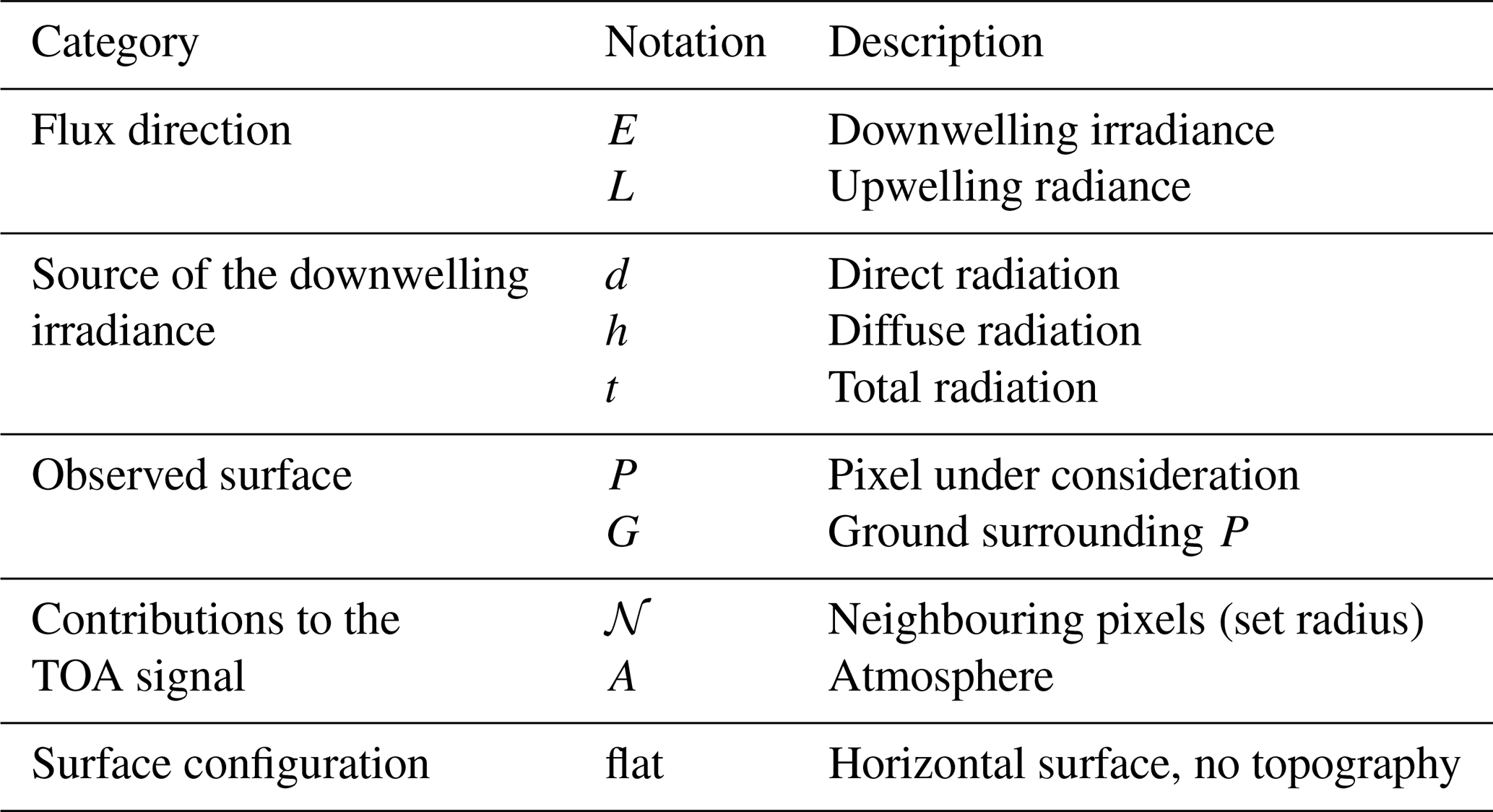
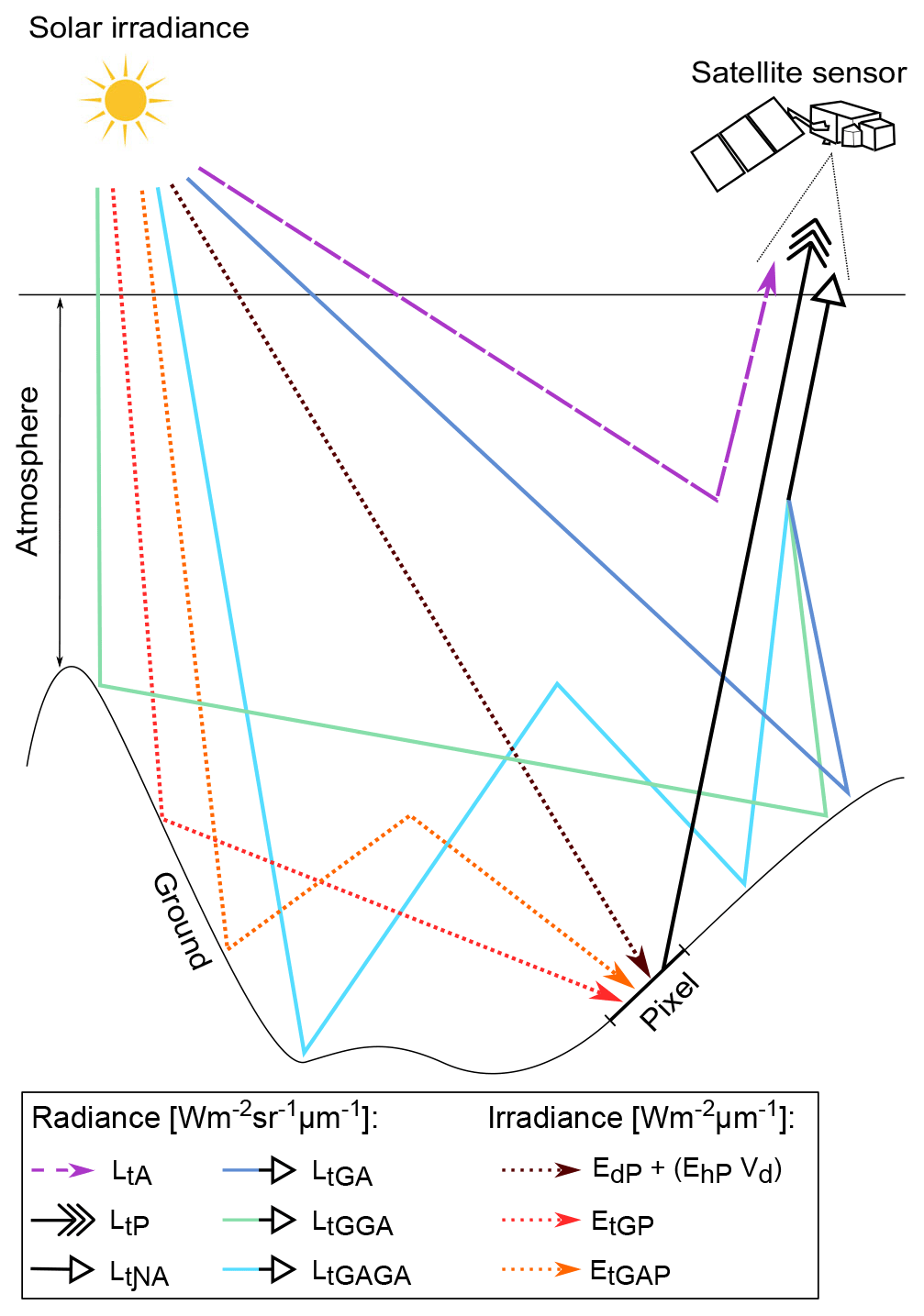
Figure 1Illustration of the contributing fluxes to the TOA radiance measured by a space-borne sensor. The dotted lines correspond to solar irradiance received by the pixel P which are then reflected towards LtP, the sensor's instantaneous field of view (IFOV); the solid coloured lines represent the contribution of neighbouring slopes to the measured signal (Lt𝒩A), and the dashed line is the atmospheric path radiance (LtA). For sake of clarity, the direct and diffuse components of the downwelling fluxes are merged in this scheme.
2.1 TOA radiance formulation over rugged terrain
2.1.1 General formulation
The forward model computing TOA radiance over snow-covered rugged terrain is based on formulations and approximations found in Lenot et al. (2009), Sirguey et al. (2009), and Kokhanovsky and Zege (2004). To derive the equations involving the numerous terms contributing to TOA radiance, a simple and rigorous notation system is introduced in Table 1 and Fig. 1. For example, following the notation system, represents the diffuse (h) downwelling irradiance (E) reaching a flat pixel under consideration (Pflat). Note that the wavelength λ is omitted from all terms for clarity.
According to Lenot et al. (2009), the total radiance of a pixel P observed by a space-borne sensor can be expressed as
where is the solar radiation reflected by the pixel P directly towards the satellite's instantaneous field of view (IFOV), is the contribution of neighbouring slopes (within a set distance to pixel P) scattered by the atmosphere to the satellite, and is the atmospheric path radiance measured by a sensor without any interaction with the surface. θi and θv describe the illumination and viewing zenith angles, respectively, and ϕi and ϕv describe the illumination and viewing azimuth angles, respectively, for a flat surface.
2.1.2 Contribution of the pixel's signal
The contribution to the TOA radiance of solar radiation reflected by the pixel P can be written as
with the direct contribution of the reflected solar beam:
where is the bidirectional reflectance factor (BRF; Schaepman-Strub et al., 2006) of the surface (here ) and is the direct atmospheric transmittance in the viewing direction, depending on the geographic location and elevation of the pixel P. The angles and are the effective (incident and viewing, respectively) zenith and azimuth angles on a sloping surface at P and are given by , with θn and ϕn the slope and aspect of the surface, respectively (Dumont et al., 2017). If the sensor has direct line of sight with the pixel P, the binary function is 1; otherwise it is 0. is the direct solar irradiance received by the surface, expressed as
with , a sub-pixel fraction of shadows (Sirguey et al., 2009), where 0 corresponds to a fully shadowed pixel and 1 to a pixel free of shadows, accounting for self shadows described by and cast shadows calculated using a DEM (Dozier et al., 1981). Eo is the extraterrestrial solar irradiance (Neckel and Labs, 1984), and is the direct atmospheric transmittance in the direction of the sun. As is the case for , depends on the location and altitude of the pixel P, as well as on the atmospheric properties.
The diffuse contribution of the reflected solar radiation by pixel P is expressed as
where av is the hemispheric–directional reflectance (HDR; Schaepman-Strub et al., 2006) of the pixel that reads
with dΩ=sin θdθdϕ. is the diffuse irradiance from the surrounding slopes and the atmosphere received by pixel P, and written as
with being the irradiance received by a theoretically horizontal surface modulated by Vd(P) and the sky-view factor (Dozier et al., 1981) varying from 0 to 1 and approximated by Dozier and Frew (1990) as
for which the horizon angle from zenith Hz(ϕ) for a given azimuth ϕ is converted as from the horizon elevation H(ϕ), itself calculated using the algorithm of Dozier et al. (1981). is the irradiance received from surrounding slopes, and is the coupled atmospheric irradiance reaching pixel P after multiple reflections by the surrounding slopes and scattering by the atmosphere. When taking into account these adjacency effects, the diffuse radiance of the pixel P (Eq. 5) at the kth iteration becomes
and is updated at each iteration k. Numerical tests over different terrain configurations in the French Alps (not presented here) have shown that the equation converges in approximately four to six iterations. When calculating the contributions from the surrounding terrain to an observed pixel, several assumptions are made in the following equations. First, it is assumed that all the pixels in the neighbourhood 𝒩 of a pixel P are receiving the same irradiance as a horizontal surface. Second, the shape of the terrain surrounding the pixel P is considered as in Dozier and Frew (1990), in that the terrain forms a bowl extending to the horizon in all azimuths (ϕ). Lastly, the surface reflectance of pixels surrounding the observed pixel is assumed to be Lambertian for simplicity; thus (see Eq. 12).
According to Sirguey et al. (2009), the solar radiation reflected once by a neighbouring slope towards the pixel under consideration can be approximated as
The total downwelling irradiance is expressed for a horizontal surface, where the diffuse solar irradiance is calculated with an atmospheric radiative-transfer model and the direct solar irradiance is expressed as
The bi-hemispherical albedo of the surface of a pixel M, S(M), located in 𝒩(P), is expressed as
where as is the surface directional–hemispherical reflectance (DHR; Schaepman-Strub et al., 2006). Similarly to Eq. (6), the DHR of a pixel M can be written as
and thus for any point X, . R is the surface hemispherical–conical reflectance (HCRF; Schaepman-Strub et al., 2006) of the pixel P, is updated with the values calculated for the previous iteration k−1 and is written as
In mountainous areas, when the trapping mechanism of reflected radiation between slopes is considered (Sirguey, 2009), Eq. (10) is modified to account for the coupling:
In the literature, the neighbourhood of reflected radiation by surrounding terrain 𝒩(P) is generally delimited by a circle of 0.5–1 km (Lenot et al., 2009; Richter, 1998; Sirguey et al., 2009). The HCRF of the pixels in the neighbourhood, , is calculated with Eq. (14).
The atmospheric coupling contributing to pixel P's illumination, which accounts for the multiple reflections between slopes (also present in Eq. 15), can also be approximated iteratively according to Sirguey et al. (2009):
with αatm denoting the atmospheric hemispherical albedo, which is the diffuse descending atmospheric component. Based on previous studies, the neighbourhood used for the contribution of pixels to the diffuse atmospheric scattering (𝒩2(P)) differs from the neighbourhood used for the effects of scattering by surrounding slopes (𝒩(P)) and is in the range of 1–2 km (Lenot et al., 2009; Richter, 1998; Sirguey et al., 2009).
2.1.3 Contributions of surrounding slopes
Following Eq. (1), the contribution of the slopes in the vicinity of the pixel under consideration to the measured TOA radiance (without any interaction with the pixel P but nevertheless a dependency on P to define the neighbourhood) can be divided into three components (Fig. 1):
where corresponds to the solar radiation scattered once by the surrounding ground and then by the atmosphere towards the sensor, is the contribution of the multiple reflections occurring between slopes, and is the coupled atmospheric multiple scattering. It follows that
where and denote the effective solar zenith and azimuth angles accounting for the local topography of pixel M. Fenv is the weight of the pixel M in the TOA radiance originating from 𝒩(P). Fenv accounts for both terrain and atmospheric effects (i.e. atmospheric transmittance) and can be calculated using a Monte Carlo approach (Lenot et al., 2009). However, the approximation of Eq. (17) used in this study (see Eq. 20) does not require such calculations. The two remaining terms of Eq. (17) are considered to be intertwined and hence are defined as
Although the different terms of Eq. (17) have been introduced separately above, Sirguey et al. (2009) have shown that the total contributions of surrounding slopes to TOA radiance can be approximated overall as
where td(θv,ϕv) is the atmospheric diffuse transmittance, expressed by Sirguey et al. (2009) as
which corresponds to the radiation scattered by the atmosphere reaching the sensor and can be calculated using an atmospheric radiative-transfer model by imposing the sensor geometry (θv,ϕv) in place of the sun angles. The environmental reflectance defined by Sirguey et al. (2009) as the spatial average of each pixel reflectance R within the neighbourhood 𝒩2 is iteratively updated:
2.2 Simplified cases of TOA radiance formulation
To provide a comparison of REDRESS output with the current approaches generally used in the literature and assess the errors introduced by neglecting the rugged-terrain effects, REDRESS was run considering a horizontal surface or slopes only, by updating the terms of the general formulation (Eq. 1) for each configuration.
2.2.1 Flat terrain
For a perfectly flat landscape, the TOA radiance is limited to the sum of the direct and diffuse downwelling irradiance reflected by the pixel's surface and the atmospheric path radiance. In this configuration, the signal measured by a space-borne sensor is expressed as
where the contribution of the reflected direct radiance is written as
and the reflected diffuse solar radiation originating from the scattered irradiance by the atmosphere only is
In this study, the simulations performed with REDRESS using the flat-terrain configuration are referred to as REDRESSflat.
2.2.2 Sloping terrain
When considering the effects of terrain slope and aspect, the flat-terrain formulation is modified to account for the local illumination and viewing angles modified by the terrain, shadowing, and the surfaces visible by the satellite sensor. Therefore, in the formulation developed in Sect. 2.2.1, Eq. (24) is replaced by Eq. (3) and Eq. (25) is replaced by Eq. (5) in which the reflected illumination and atmospheric–terrain coupling are neglected. Thus, in Eq. (5) the diffuse contribution of the downwelling solar radiation (Eq. 7) is reduced to
The simulations performed with REDRESS accounting for the first-order slope effects only are denoted by REDRESSslope hereinafter.
The section first presents the implementation of the model, followed by the data and methods used to validate the model.
3.1 Model implementation
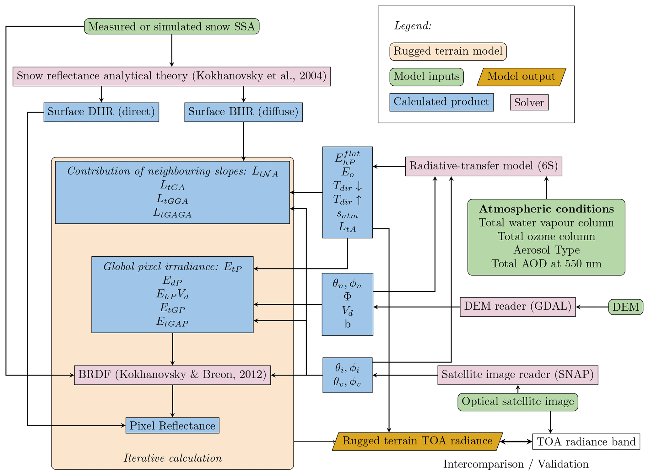
Figure 2Processing steps to simulate TOA radiance over snow-covered rugged terrain. The model input products (green boxes) and the variables (blue boxes) are used in the iterative process (beige box) that calculates TOA radiance (orange lozenge). The pink boxes represent the interchangeable modules in the model, with the formulation used in this study in brackets.
The equations in Sect. 2 form a forward model aiming to solve Eq. (1) and thus generate synthetic TOA spectral radiance images over snow-covered mountainous terrain as measured by an optical space-borne sensor. The model was implemented in Python with an architecture organised around interchangeable modules (Fig. 2, pink boxes) designed to be easily replaced, allowing the application of different formulations at each different computation stage. The processing workflow consists of five modules that read and process the input data (green in Fig. 2), providing the model's configuration parameters, and one core module (beige box in Fig. 2) that performs the iterative forward calculations of TOA radiance. The four main data sources required to run the model and the modules used to process the inputs, as well as the main module, are described in the following sections.
3.1.1 Satellite sensor configuration
Information about the satellite's sensor configuration is used as inputs to the forward model, enabling a direct comparison between the model outputs and TOA radiance measured by a specified satellite sensor. The data extracted from the satellite product include θi,ϕi and θv,ϕv; the illumination and viewing angles at the time of the overpass; the spatial resolution; and the spectral characteristics of the sensor. For each spectral channel, the radiance is computed with a 1 nm wavelength step and integrated using the spectral response function of the satellite bands. In this study, the module used to read the satellite data is based on the Python API of the ESA Sentinel Application Platform (SNAP; http://step.esa.int, last access: 9 September 2020), but other reading modules can be easily implemented.
3.1.2 Snow physical properties
Specific surface area (SSA) is one of the main drivers of snow reflectance. It is a metric directly related to the optical diameter of snow grains that is widely used in remote sensing of snow (e.g. Dozier, 1984; Scambos et al., 2007; Painter et al., 2009). The current version of the model relies on the assumption that the SSA is known and constant across the scene. The SSA is used as an input of the asymptotic analytical radiative-transfer theory, to compute surface directional–hemispherical reflectance (DHR, a.k.a. black-sky albedo) and bi-hemispherical reflectance (BHR, a.k.a. white-sky albedo) and the BRF of the snow surface (Kokhanovsky and Zege, 2004; Kokhanovsky and Breon, 2012). The resulting BRF is used to compute the direct contribution of the reflected solar beam for each pixel, as shown in Eq. (3). It should also be noted that in the current version of REDRESS, snow is considered to be free of impurities, such as black carbon or mineral aerosol deposits.
3.1.3 Atmospheric properties
The atmospheric components are calculated using the 6S radiative-transfer model (Vermote et al., 1997) that is initialised with four main parameters: water vapour content, the total ozone column, the type of aerosol present in the atmosphere, and the total aerosol optical depth (AOD) obtained from the datasets described in Sect. 3.2.4. Additionally, 6S takes as inputs θi and ϕi, θv and ϕv, the solar and viewing angles extracted from the satellite product, and the ground elevation obtained from the DEM. The model provides the required atmospheric inputs of REDRESS, which include Eo, the extraterrestrial solar irradiance; , the diffuse downwelling irradiance at the surface; and , the atmospheric transmittance in the solar and viewing directions; as, the atmosphere's spherical albedo, LtA; the atmosphere's intrinsic radiance; and the direct-to-diffuse illumination ratio at the surface. In the current setup, REDRESS, written in python, uses the Py6S module (Wilson, 2013) to run the 6S Fortran code, but the model is designed for the easy implementation of other radiative-transfer codes.
3.1.4 Topographic parameters
A DEM is used to compute all the topographic parameters as follows. The slope and aspect of the terrain across the scene (θn,ϕn) are computed using the third-order finite difference weighted by the reciprocal of distance of Horn (1981). The algorithm, which has been shown to represent slope and aspect more precisely than other approaches (Lee and Clarke, 2005), does not overestimate the slopes or exaggerate peaks, although a loss in local variability is observed (smoothing of small dips and peaks). The fraction of sky masked by surrounding relief for a given point is described by the sky-view factor (Dubayah and Rich, 1995), which is calculated using the DEM-based horizon algorithm of Dozier et al. (1981). As described in further detail by Sirguey et al. (2009), the horizon algorithm is run for each cell of the DEM in 64 azimuth directions to compute the horizon elevation angle, which in turn is used to determine the sky-view factor (Eq.7). The horizon algorithm is also used to compute shadows, represented by a binary map where 0 represents a shadowed pixel and 1 a sunlit pixel. The total shadow product is the combination of self shadows (i.e. slopes that do not face the sun) and cast shadows (i.e. areas where solar radiation is blocked by surrounding features). Self shadows are usually found where the cosine of the effective solar zenith angle is negative. However, visual comparisons with high-resolution imagery showed that using a slightly positive cut-off value (0.035) to account for the inaccuracies in the DEM allows a better representation of self shadows. Cast shadows are defined here as the areas where the horizon elevation angle in the direction of the sun is larger than the solar zenith angle. Noise and isolated pixels are removed by applying a 3×3 binary dilatation–erosion step (using the Python functions scipy.ndimage.morphology.grey_dilation and scipy.ndimage.morphology.grey_erosion) to the cast-shadow map. All the topographic products are first calculated at the DEM resolution and then are resampled to the satellite resolution and in the geometry of acquisition of each image. The resampling steps are performed in the code using the GDAL library (GDAL/OGR contributors, 2019).
3.1.5 Iterative forward module
Using the inputs described in the previous sections, the TOA radiance of each pixel across the scene is calculated iteratively. To start, the BHR of the snow is used as a first guess in the iteration process for the diffuse environmental reflectance and the radiation reflected by the adjacent slopes. The terms are updated at each iteration from the calculated HCRF (Eq. 14) averaged with a sliding window of the size of the neighbourhood contributing to the pixel (Eqs. 15 and 16). In turn, the radiance of the neighbouring terrain (Eq. 17), the diffuse contribution of the reflected solar radiation (Eq. 5), and the total radiance (Eq. 1) are updated. Numerous calculations over different datasets have shown that the iteration process convergence is rapid, with on average four to six iterations over a typical alpine scene with pronounced topography. The iterative process is terminated when the average difference in radiance across the scene is less than 0.1 % between two consecutive iterations.
3.2 Study site and data
3.2.1 Study site
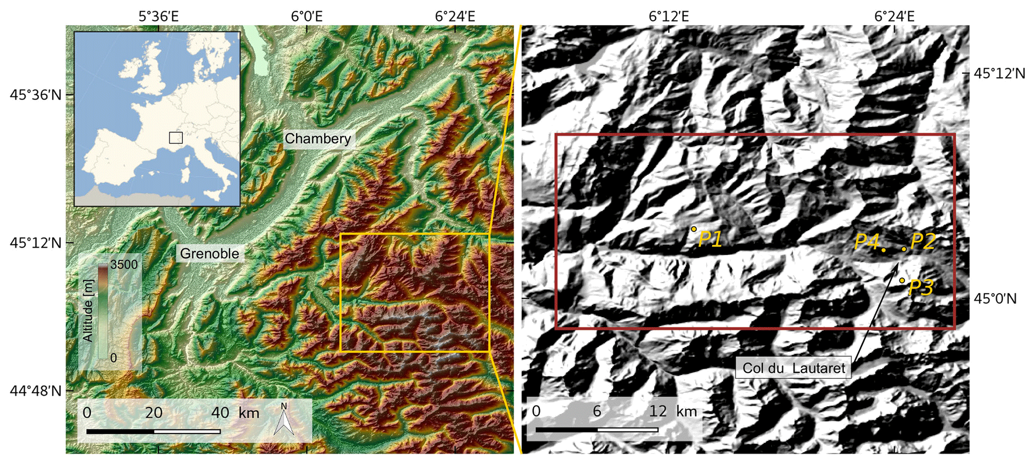
Figure 3Location of the Col du Lautaret experimental site. The extent used for the validation of the model is outlined in red, over the hillshade product generated from and draped over the 30 m ASTER DEM. The four individual sites are marked as yellow dots. (Europe map source: Alexrk2/Wikimedia Commons, modified under the Creative Commons Attribution-Share Alike 3.0 Unported license).
Table 2Summary of the four selected pixels across the study site. Note that aspect is measured clockwise, with 0∘ representing the north.
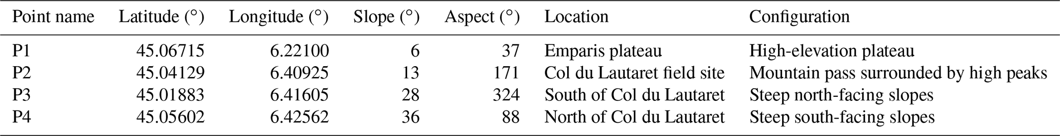
A study area covering approximately 17 km × 20 km in the southwestern French Alps was selected for the evaluation of the model (Fig. 3). The region is composed of narrow valleys surrounded by steep slopes, with elevations ranging from 1520 to 3983 m. The extent includes Emparis (45∘04′ N, 6∘14′ E), a large grass plateau with moderate relief located at an elevation of approximately 2000 m, and Col du Lautaret (45∘02′ N, 6∘24′ E), a high-altitude mountain pass that reaches an elevation of 2058 m, characterised by a wide open area above the treeline surrounded by high mountain peaks. To highlight specific terrain configurations and examine the spectral performance of the model, four individual sites were selected across the scene (shown in Fig. 3). The first point, P1, is located on the Emparis plateau and is the closest configuration to flat terrain, with slightly sloping terrain and very little contribution from nearby features. P2 is located on a small plateau at the Col du Lautaret site, where field measurements were acquired (see Sect. 3.2.3). The pixel P2 presents small slopes with nevertheless an important contribution of the surrounding topography. The third site, P3, located to the south of the Col du Lautaret pass, is characterised by a steep north-facing slope and is fully shadowed. Lastly, P4 is located on a sunlit south-facing slope located to the north of the Col du Lautaret where the direct solar radiation dominates the signal. A summary of the four locations and their characteristics is presented in Table 2.
3.2.2 Satellite data
Table 3Summary of the Sentinel-3A OLCI satellite acquisitions and the field measurements obtained for clear-sky conditions during the 2017/18 winter season. For each date the start and end times of the acquisition are indicated. The viewing and solar angles shown here were averaged across the scene. The average measured SSA across the transect is indicated with ± 1σ representing the spatial variability in the SSA across the site.
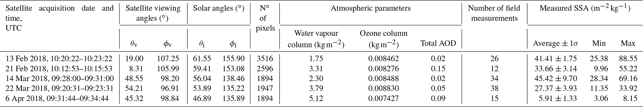
The OLCI sensor on board Sentinel-3 is a push-broom imaging spectrometer that covers the spectral range of 400–1020 nm with 21 bands and has a spatial resolution of approximately 300 m at nadir. The instrument provides a high repeat coverage, with a revisit time of less than 2 d in the French Alps, and a large spatial coverage thanks to a swath width of 1270 km, providing an ideal tool for monitoring the dynamics of alpine snow. The TOA values of atmosphere radiance simulations for the aforementioned study area were compared to five Sentinel-3A OLCI L1 full-resolution scenes acquired between 13 February 2018 and 6 April 2018. Overpass dates were selected based on two criteria: the absence of clouds, which was visually assessed on-site, and the acquisition of concurrent surface SSA measurements in the field. The five dates matching the criteria cover a wide range of snow conditions from winter to spring and were acquired with different solar and viewing geometries, allowing the validation of the model for a wide range of acquisition conditions. For the detailed evaluation purposes in Sect. 4.1, the scene acquired on 13 February 2018 was retained, as it contained the most snow-covered pixels. A summary of the satellite acquisitions is presented in Table 3.
3.2.3 Field measurements
Ground measurements were collected during the Sentinel-3 overpass for the five dates. The SSA of snow samples taken at the surface of the snowpack was measured across the Col du Lautaret site using the Alpine Snowpack Specific Surface Area Profiler (ASSSAP; Arnaud et al., 2011), which has an estimated accuracy of 10 %. The measurements taken on 13 and 21 February, 14 March, and 6 April were carried out on a small plateau located on the south-facing slopes to the north of the site, crossing pixel P2, whereas on 22 March SSA measurements were acquired across the north-facing slopes located on the south side of Col du Lautaret pass, approximately halfway between P2 and P3. For both sites, the measurements were taken along transects covering a variety of slopes and orientations and thus snow conditions. SSA samples were measured every 20 m along the transects. The regular spacing between the points was ensured by using a 20 m rope, and the start and end points of each transect were geolocalised using a handheld GPS device with an estimated accuracy of ± 5 m. The result of the measurements are given in Table 3.
3.2.4 Model setup
For each Sentinel-3 OLCI acquisition, TOA radiance was simulated for the 21 spectral bands using REDRESS. The model was run using the ancillary data from the Sentinel-3 acquisition as input parameters: solar and viewing zenith and azimuth angles, sensor characteristics, and the spectral-band response functions. The average SSA measured along the transect was used as a single input SSA value, given that in the current model setup, snow is described using a fixed SSA value across the scene. The topography was obtained from the Advanced Spaceborne Thermal Emission and Reflection Radiometer (ASTER) Global Digital Elevation Model (GDEM) Version 3 (NASA/METI/AIST/Japan Spacesystems, 2019), with a spatial resolution of 1 arcsec (approximately 30 m). The DEM was selected for its suitable resolution for the computation of topographic parameters in mountainous regions (Frey and Paul, 2012) and its widespread availability. The input parameters for the radiative-transfer calculations performed with Py6S were obtained from different sources. The Copernicus Atmosphere Monitoring Service (CAMS) near-real-time analysis dataset provides daily analyses of atmospheric conditions and aerosol content with a horizontal resolution of 0.4∘ (approximately 31 km × 44 km). The total column ozone, total column water vapour, and total aerosol optical depth (AOD) at 550 nm were extracted from this dataset for each OLCI product. For all the simulations, the aerosol model was set to the standard 6S “Continental” model (Vermote et al., 2006). The radiative-transfer model was run twice for the entire study area: a first time with the average viewing and illumination geometries of the scene and a second time inverting the viewing and illumination geometries to compute the missing parameters (e.g. Eq. 21). Finally, the iterative model was run with the environmental reflectance neighbourhood 𝒩2 (see Eq. 16) set to 2.1 km and the neighbourhood of the radiation reflected by surrounding terrain, 𝒩 (see Eq. 15), set to 1.5 km, which were found to yield the best results for the selected scene.
The current implementation of the model only considers snow-covered pixels and does not account for fractional snow cover. Therefore, for validation purposes, the TOA radiance was not modelled for pixels containing less than 80 % of snow. The snow cover percentage was obtained by calculating the proportion of Theia Snow collection pixels (Gascoin et al., 2019), based on Sentinel-2 images at a resolution of 20 m, within each Sentinel-3 OLCI pixel. Due to the lower revisit time of Sentinel-2 (5 d), the closest available date to the OLCI image was used, and cloud-covered areas were filled with the next-closest date.
3.3 Surface reflectance
Surface reflectance retrieved from TOA radiance satellite observations is a common product of interest which is more widely used in Earth observation than TOA radiance itself. Although the inversion of surface reflectance was not performed in REDRESS, a first estimation of the impact of the complex topographic effects on future retrievals is proposed by converting the TOA radiance simulations to bottom-of-atmosphere (BOA) HCRF (hereinafter referred to as reflectance) by removing the atmospheric terms. This conversion was performed for the scene on 13 February 2018, first for REDRESS simulations and then considering the effect of slopes only. The surface reflectance was obtained from TOA radiance using Eq. (14), which removes the atmospheric terms. For the slope-only configuration, Eq. (14) was modified to remove the contribution of neighbouring terrain (Eq. 17) and the reflected solar radiation from neighbouring slopes (Eq. 10), thus becoming
3.4 Sensitivity analysis
Table 4Range of values used to evaluate the sensitivity of the TOA simulations to the model input parameters.
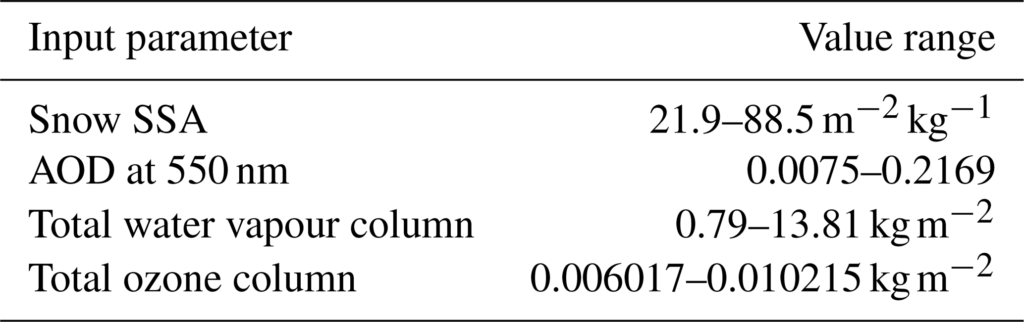
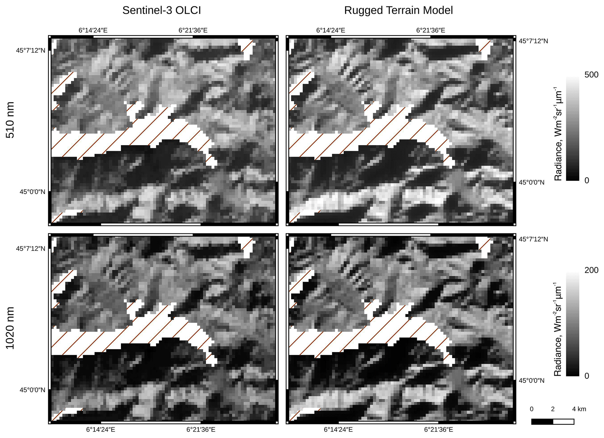
Figure 4TOA radiance image observed by Sentinel-3 OLCI L1B (© Copernicus) acquired on 13 February 2018 (left) and simulated with the rugged-terrain model (right) at 510 nm (top) and 1020 nm (bottom). Pixels containing less than 80 % of snow were masked out (hatched region).
To evaluate the sensitivity of the TOA simulations to the model input parameters, the rugged-terrain model was run for varying values of snow SSA, AOD, total column water vapour, and total ozone column, reported in Table 4. The simulations were performed with the configuration of 13 February 2018. During the simulations over a range of values for each input parameter, the other inputs were fixed to the values reported in Table 3. The range of values was taken for snow SSA from the minimum and maximum values measured in the field over the snow season 2017–2018 and for the atmospheric parameters from the minimum and maximum values in the CAMS near-real-time analysis dataset between December 2017 and April 2018.
The performance of REDRESS is first evaluated by comparing in detail the model output to the Sentinel-3 OLCI TOA radiance image acquired on 13 February 2018 (Sect. 4.1) and second by extending the comparison to five Sentinel-3 OLCI acquisitions over an entire winter season (Sect. 4.2). Finally, the sensitivity of the model results to the input parameters is investigated (Sect. 4.3).
4.1 Model performance on a single date
4.1.1 Spatial comparison at two wavelengths
Figure 4 shows a Sentinel-3 OLCI L1B image subset covering the study area (red box in Fig. 3) acquired on 13 February 2018, compared to a TOA radiance synthetic map produced with REDRESS at 510 nm (band 05) and 1020 nm (band 21). The observations and simulations highlight that the TOA signal is dominated by the complexity of the topography and that the range of observed TOA radiance values is indeed high for seemingly uniform snow-covered surfaces. A correlation larger than 0.7 associated with low bias (5–10 ) between the measured and modelled TOA radiance is observed at both wavelengths, highlighting the model's ability to reproduce the large variations in TOA radiance across the scene despite the same intrinsic snow properties being applied to all pixels. Indeed, the spatial pattern between the satellite and synthetic images is similar, with dark-shaded areas located on north-facing slopes and brighter south-facing slopes (at the time of the acquisition, the sun was located south-southeast; see Table 3). Nevertheless, the variations in TOA radiance are more pronounced in the synthetic image, which has a slightly larger value range (45–511 at 510 nm, 2–181 at 1020 nm) than that of the satellite image (36–456 at 510 nm, 2–162 at 1020 nm), and cause the scene to appear sharper. At both wavelengths, the TOA radiance of south-facing slopes (i.e. in the southern part of the images) is weakly overestimated by the model, making them appear brighter than in the satellite image, whereas shadows located on north-facing slopes are less gradual than in the satellite image and form denser dark areas where the TOA radiance is underestimated.
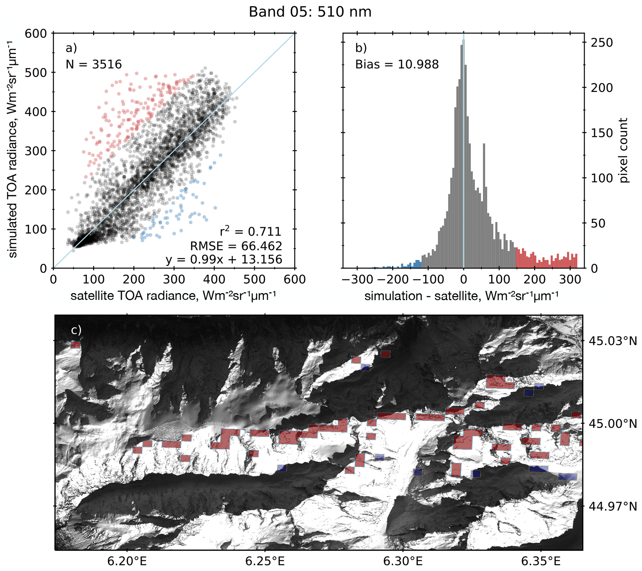
Figure 5TOA radiance spectra computed with the rugged-terrain model and observed with OLCI at 510 nm (band 05) on 13 February 2018. (a) Scatterplot of the relationship between the simulated TOA radiance and the concurrent satellite observations over the study area. The coloured points (red and blue) represent values under- or overestimated by more than 2σ of the bias. (b) Difference between simulation and observation across the scene. (c) Spatial distribution of the under- and overestimated pixels shown on a 1.25 m resolution SPOT 6 image, acquired on 19 February 2018 at 10:04 UTC via the Kalideos Alpes project (© AIRBUS DS).

Figure 6TOA radiance spectra computed with the rugged-terrain model and observed with OLCI at 1020 nm (band 21) on 13 February 2018. (a) Scatterplot of the relationship between the simulated TOA radiance and the concurrent satellite observations over the study area. The coloured points (red and blue) represent values under- or overestimated by more than 2σ of the bias. (b) Difference between simulation and observation across the scene. (c) Spatial distribution of the under- and overestimated pixels shown on a 1.25 m resolution SPOT 6 image, acquired on 19 February 2018 at 10:04 UTC via the Kalideos Alpes project (©AIRBUS DS).
To illustrate the performance of the model, the scatterplots and bias histograms between the measured and synthetic images are shown for the study area at 510 nm (Fig. 5a and b) and 1020 nm (Fig. 6a and b). At both wavelengths, the values are densely distributed along the identity line, with a correlation of 0.71 at 510 nm and 0.73 at 1020 nm. The bias is low (11 at 510 nm and 6.7 at 1020 nm), and the histogram of the model errors reveals a peaked, nearly centred distribution with a long tail skewed towards the positive values (overestimation of the model), as well as a smaller tail covering negative values. To identify the spatial distribution of the pixels for which the bias between the model and the satellite observations was the highest, the values over- and underestimated by more than 2 SDs of the bias were coloured in red and blue, respectively, and identified as such in all the panels of Figs. 5 and 6. An enlarged subset of the overlay of the corresponding pixels is shown on a high-resolution panchromatic SPOT 6 image acquired on 19 February 2019, 6 d after the OLCI scene and at a similar time of day (Figs. 5c and 6c). At both wavelengths, the pixels overestimated by the model are distributed along ridgelines or buttresses, where a change in the slope and aspect is observed, and the pixels underestimated by the model are located on the edge of projected shadowed areas. Removing the red and blue areas from the analysis significantly improves the correlation, yielding r2 = 0.84 at 510 nm and r2 = 0.86 at 1020 nm. However, in this study all the pixels were kept for the analysis.
4.1.2 Band-wise comparison at four locations
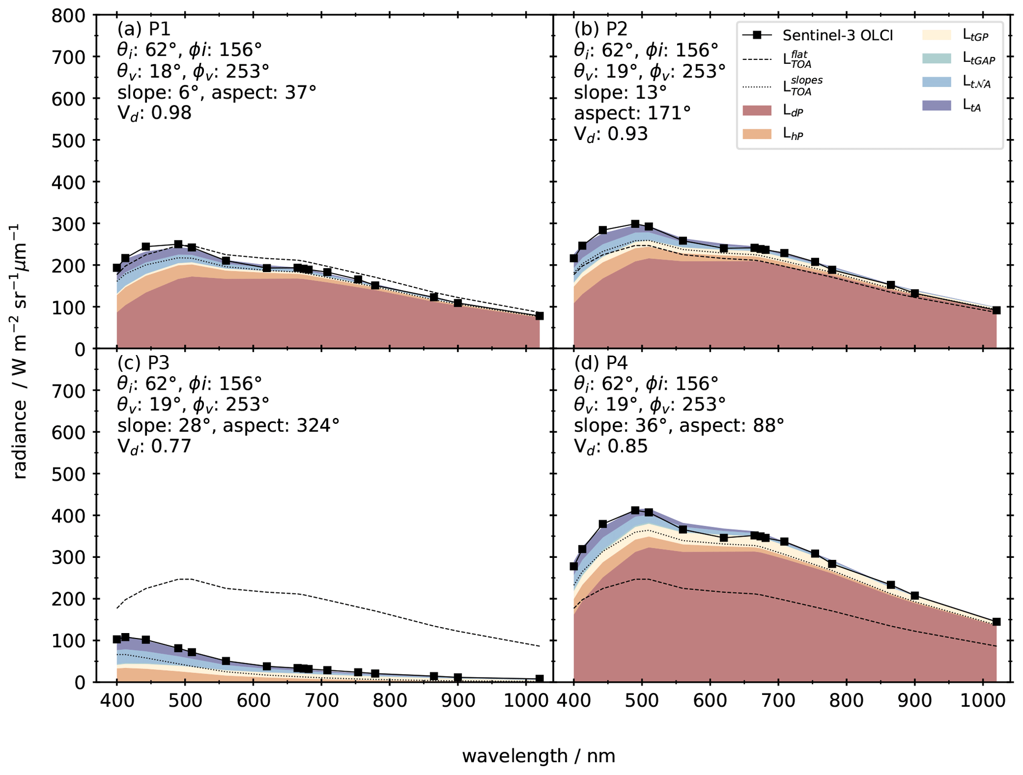
Figure 7TOA radiance observed by Sentinel-3 OLCI (L1B) and simulated by REDRESS considering the full-rugged-terrain problem (stacked coloured spectra), slopes only (dotted lines), and a flat surface (dashed lines), for 4 pixels with different terrain configurations on 13 February 2018. Note that values for LtGAP are too small to appear on the graph.
The comparison between the TOA radiance spectra measured by Sentinel-3 OLCI and simulated using REDRESS on 13 February 2018 is shown in Fig. 7 for 4 pixels located across the study site (Fig. 3). As was the case for the two individual wavelengths in Fig. 4, a good agreement between the REDRESS-simulated spectra and the TOA radiance measured by Sentinel-3 OLCI is observed at all wavelengths, despite the different terrain configuration of the 4 pixels (Table 2). To assess the errors caused by neglecting the full effects of rugged terrain, simulations considering a flat surface (REDRESSflat) and slopes (REDRESSslope) are represented by dashed and dotted lines, respectively. In the case of the pixel P1 (Fig. 7a), which is the closest to a flat surface, the modelled TOA radiance with REDRESSflat is, as expected, close overall to the satellite measurement, with a mean absolute error (MAE) of 9.8 . Modelling the TOA radiance with REDRESSslope slightly improves the results compared to flat terrain above 510 nm but underestimates the signal at shorter wavelengths, leading to an increased MAE of 16.2 . Even in such a configuration with small slopes (< 10∘) and negligible reillumination from neighbouring slopes, running REDRESS largely improves the simulation results, with an MAE of 3.1 . For terrain configurations with slightly larger slopes and pronounced surrounding features such as P2 (Fig. 7b), accounting for the slopes brings improvement over considering a flat terrain (MAE of 21.1 and 38.1 , respectively) across all spectral bands but, similarly to the other sites, underestimates the measured TOA signal. In comparison, REDRESS simulations perform well, with an MAE of 4.8 . In more extreme cases, the flat-terrain assumption leads on the one hand to a significant overestimation of the TOA radiance on steep north-facing shadowed slopes (P3, Fig. 7c) mainly because it does not consider shadowing due to relief, resulting in an MAE of 102.8 . On the other hand, the TOA radiance of strongly reilluminated south-facing slopes (P4, Fig. 7d) is underestimated by REDRESSflat, with an MAE of 126.1 . Accounting for slopes shows a better agreement with the satellite measurements; however the lack of consideration of multiple reflections between the pixel and surrounding slopes, as well as of the atmospheric and terrain coupling, leads to a systematic underestimation of the measured TOA signal (MAE of 23.4 for P3 and 30.7 for P4). REDRESS is able to simulate the large variations from a pixel to another, satisfactorily reproducing the satellite measurements, with an MAE of 1.7 for P3 and 7.3 for P4. Despite a good overall agreement, small discrepancies are observed in the range of 510–620 nm, which may be explained by uncertainties in the parameterisation of the atmospheric ozone content in the radiative-transfer module, as highlighted in Sect. 4.3.
4.1.3 Contributing terms to TOA radiance in snow-covered rugged terrain
The discretisation of the different terms making up the TOA radiance simulated with the full-rugged-terrain model underlines the spectrally dependent contribution of the terms to the overall signal. For the sites P1, P2, and P4, located in direct sunlight, the reflected direct sunlight (LdP) is of the first order, dominating the signal in the near-infrared domain (between 90 % and 95 % at 1020 nm) and making up almost half the signal in the blue range of the spectrum (between 44 % and 56 % at 400 nm). Furthermore, the slope has a strong influence on the intensity and spectral shape of LdP, in turn largely impacting the overall spectral shape of the total TOA radiance (Picard et al., 2020). P3 differs strongly from the other sites owing to its position on a self-shadowed slope, leading to LdP being null. All the other components of the reflected solar radiation are diffuse and therefore contribute decreasingly to the total signal as a function of wavelength between the blue and near-infrared wavelengths. The reflected sky radiation (LdP) depends on the proportion of sky “seen” by the pixel, expressed by Vd (Eq. 7, shown in Fig. 7). Indeed, the contribution of LhP is more important in an open area such as P1, with Vd = 0.98 (41 at 400 nm), than for P3, with Vd = 0.77 (34 at 400 nm), which is located in the middle of a steep slope and thus with part of the sky masked by its own slope as well as by surrounding slopes. The contributions of the multiple reflections from surrounding slopes and the coupled terrain–atmosphere reflections (LtGP and LtGAP) largely depend on the terrain surrounding the observed pixel. Hence, the contributions of surrounding slopes are small for the flat plateau on which P1 is located, with a maximum of 5 at 490 nm, whereas for P4, surrounded by large slopes, the contribution reaches 33 . For the four sites presented in Fig. 7, LtGP makes up most of the contribution from the surrounding terrain, whereas LtGAP is negligible. The neighbouring pixels' diffuse and coupled atmospheric contribution (Lt𝒩A) is similar for all sites, varying between 31 (P1) and 33 (P4) at 400 nm. Lastly, for all sites, the contribution of the atmosphere intrinsic radiance is commensurate for all pixels, as it depends on the illumination and viewing geometries, the altitude of the pixel, and the atmospheric composition, which are all similar for the four sites.
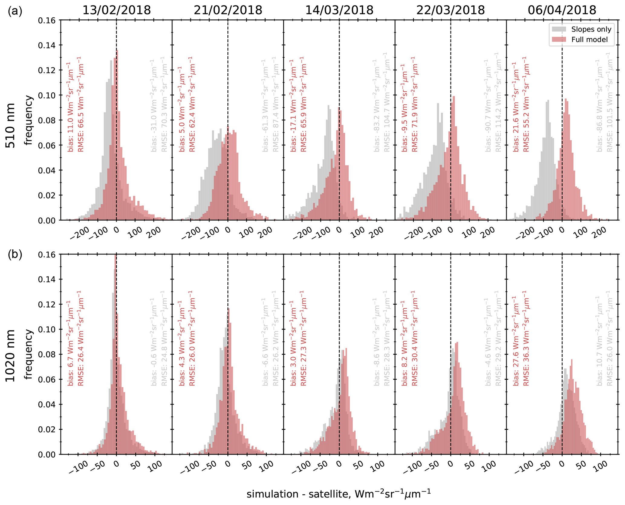
Figure 8Distribution of the difference in TOA radiance between REDRESS simulations (red) and Sentinel-3 OLCI observations at band 05 (510 nm, a) and band 21 (1020 nm, b) for the five dates in 2018 over the study area. In grey is the same for simulations run considering slopes only. The bias and RMSE for REDRESS and REDRESSslope are indicated in each panel in red and grey, respectively.
Over snow-covered surfaces, all the terms making up the TOA radiance are of the same order of magnitude, except the terrain–atmosphere coupling (multiple reflections between slopes) which is negligible. Therefore to correctly infer information about the surface from space-borne images, all of the following terms need to be considered: (i) the slope and aspect of the surface, (ii) reillumination from neighbouring slopes, and (iii) atmospheric scattering into the sensor's field of view. Neglecting the last two terms leads to significant underestimations of the TOA radiance.
4.2 Model performance over a winter season
To assess the performance of REDRESS over a snow season, the model was applied to the five Sentinel-3 OLCI acquisitions between 13 February and 6 April 2018. The results are presented in the form of the distribution of the difference between the model outputs and Sentinel-3 OLCI images at 510 and 1020 nm in Fig. 8. In order to gauge the benefits of using the REDRESS model over more common approaches considering the first-order effects of slopes only, the figure also shows the bias distribution of simulations performed with REDRESSslope. Similarly to Fig. 4, pixels containing less than 80 % of snow were discarded from the analysis. Thus, the number of pixels used for the comparison has a decreasing trend throughout the season owing to snowmelt (Table 3).
4.2.1 REDRESS simulations
The bias distribution between REDRESS simulations and Sentinel-3 OLCI images shown in Fig. 8 is similar for the five dates in 2018, demonstrating the model's consistency in simulating TOA radiance for a variety of snow cover and properties conditions. Thus, it is reasonable to consider the performance analysis in Sect. 4.1 to be representative of the simulations performed throughout the winter season. At 510 nm, the bias remains low for the first four dates, ranging from 5 on 21 February 2018 to −17 on 14 March 2018. The slightly more pronounced overestimation of REDRESS observed on 6 April 2018 (22 ) could be attributed either to a misrepresentation of the snow cover in the Theia Snow collection product used to mask snow-free pixels or to the presence of impurities in the snow. The RMSE values are consistent between the dates ranging from 55 to 72 . No seasonal trends in the simulation errors are evident at 510 nm (band 05), the trend of which is similar to that of the range 400–865 nm (data not shown here).
Conversely at 1020 nm, the bias between REDRESS and the Sentinel-3 OLCI images is low (< 7 ) between 13 February and 14 March 2018 and then increases towards the end of the snow season as the error distribution shifts towards an overestimation of the TOA radiance. For the last two dates, a slight overestimation of the model is observed, with bias values of 8 and 28 on 22 March and 6 April 2018, respectively. Furthermore, a widening of the distribution of the errors manifesting itself as smaller centred peaks in the histograms and a steady increase in RMSE (from 26 on 13 February 2018 to 36 on 6 April 2018), and which does not occur at shorter wavelengths, is observed throughout the season. This trend may be explained by the increase in SSA variability that generally occurs in the spring (Bühler et al., 2015) and that is not accounted for in the model. Indeed, spatially heterogeneous SSA values may cause the measured SSA at the Col du Lautaret site to be unrepresentative of the snow conditions present across the study site, potentially playing a role in the overestimation of the TOA radiance in the near infrared.
4.2.2 Comparison with the first-order slope approach
At 510 nm, the distribution of the errors REDRESSslope has a similar pattern to that of REDRESS, and no significant difference in correlation is observed from one model configuration to the other. However, only considering the slopes leads to a systematic underestimation of the TOA radiance, which may be explained by the lack of consideration of additional solar radiation received by the pixel coming from surrounding slopes and scattered by the atmosphere. This underestimation becomes larger as the season advances, most likely owing to an increasingly higher solar position resulting in increased multiple reflections between slopes, which were correctly estimated by REDRESS. Improvements in bias going from REDRESSslope to REDRESS simulations range between 20 and 81 , reducing the bias values to the range of −17 to 22 . These improvements in bias are of the same order in the range of 400–865 nm (not shown here). Furthermore, the RMSE is increasingly improved between model configurations throughout the season in connection to the trend in bias observed, with a decrease of 4 on 13 February 2018 and 46 on 6 April 2018, leading to values of 66 and 55 for the respective dates.
As was the case at 510 nm, the error distribution between REDRESS and REDRESSslope at 1020 nm is similar, with a slightly negative bias obtained with REDRESSslope for all dates except the last. Both model configurations perform closely for the first three dates, with bias values of −1, −7, and −9 observed with REDRESSslope vs. 7, 4, and 3 with REDRESS, which improves the results slightly on 21 February and 14 March 2018. The improvements in bias are less pronounced at 1020 nm than at shorter wavelengths, which may be explained by the smaller proportion of diffuse solar radiation in the infrared. The RMSE values remain similar (< 2 ) for the two configurations. For the last two dates, REDRESS overestimates the TOA radiance by a larger amount than REDRESSslope. The overestimation is particularly marked on 6 April 2018, where the bias of REDRESSslope (11 ) is more than halved compared to REGRESS, and the difference in RMSE between the model configurations is 10 . However, if the assumption of an unrepresentative SSA value at the end of the season holds true, the systematic underestimation of TOA radiance observed on the other dates with REDRESSslope would be compensated by this effect, thus deceivingly reducing the bias.
4.3 Sensitivity to input parameters
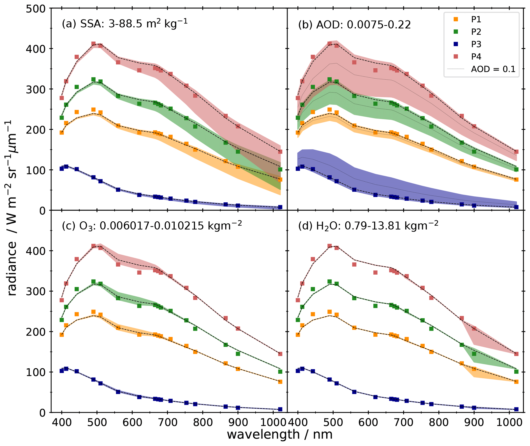
Figure 9Sensitivity of the rugged-terrain TOA radiance to the model input parameters for 4 pixels on 13 February 2018. Sentinel-3 OLCI L1B observations (coloured squares) are compared to REDRESS simulations using the parameters described in Table 3 (dashed lines) and varying (a) SSA input values, (b) AOD values (for clarity an intermediate value of 0.1 is represented as a dotted black line), (c) atmospheric ozone column values, and (d) atmospheric water vapour values (coloured envelopes).
The impact of the model's input parameters on the simulated TOA radiance is shown in Fig. 9 for the 4 pixels located across the study site (Table 2) on 13 February 2018. The Sentinel-3 OLCI TOA radiance (coloured squares) is compared to the simulations based on the values indicated in Table 3 (dashed lines) and considering a range for each parameter (Table 4; shaded areas). The variations in SSA between 3 and 88.5 , which correspond to a range of snow conditions from melting spring snow (6 April 2018) to freshly deposited wind-blown snow (13 February 2018), have an increasingly large influence on the TOA radiance between 500 and 1020 nm, with a maximal effect at 1020 nm as expected (Warren and Wiscombe, 1980). The influence of SSA on TOA radiance is closely linked to the terrain configuration. At 1020 nm, the TOA radiance varies across the SSA range by 91 for P4, 66 for P2, 45 for P1, and 5 for P3. The percentage difference between the TOA radiance calculated with the minimum and maximum SSA values is similar for pixels P1 (74 %), P2 (78 %), and P4 (80 %) but slightly higher for the steep shadowed pixel P3 (97 %). Over the wavelength range of 865–1020 nm, the modelled TOA radiance using the average SSA value measured in the field fits well the measured TOA for all sites, with a small bias of 17 for P2, which is unexpected, as the SSA was measured at that location. This discrepancy may be explained by the fact that the SSA measured along the transect on 13 February 2018 was sampled from a heterogeneous snowpack at the metre scale, spanning a wide range of values, from 21.9 to 88.5 m2 kg−1 (Table 4), and therefore the average SSA value (41.5 m2 kg−1) was not representative of the pixel. At P3 this SSA range causes a 21 variation in TOA radiance at 1020 nm (data not shown here), underlining the challenges of characterising surface snow properties at a 300 m scale.
Contrarily to SSA, variations in aerosol optical depth (AOD) have a large impact on the TOA radiance throughout the wavelength range (Fig. 9b). The TOA radiance decreases between simulations with an AOD of 0.0075 and 0.2169 for the sites P1, P2, and P4, which are located in direct sunlight, with a stronger effect on pixels with larger slopes (P4 > P2 > P1). Indeed, the TOA radiance decreases when going from the minimum to the maximum AOD by a factor of approximately 1.3 for P4, 1.05 for P1, and 1.15 for P2. This increase is of the same order at all wavelengths. In contrast the shadowed pixel P3 benefits from increased scattering in the atmosphere, and thus the TOA radiance increases by a factor of 1.5 at 400 nm to 3.5 at 1020 nm when going from an AOD of 0.0075 to 0.2169. Furthermore, at P3 the change is an increasing function of the wavelength. The results suggest that AOD was correctly predicted by the CAMS product on 13 February 2018, as the simulated TOA radiance using the reanalysis value of 0.019 closely matches the measured spectra. Nevertheless, the large change introduced by varying the AOD highlights the importance of correctly parameterising or retrieving the AOD in the atmospheric radiative-transfer model.
Ozone and water vapour in the atmosphere (Fig. 9c and d, respectively) have an effect on a limited number of bands only. Variations in ozone affect the TOA signal between 490 (band 4) and 681.25 nm (band 10). As observed for SSA, the relative variations in TOA radiance with regard to the ozone total column in the atmosphere are similar for the four studied sites. For pixel P3, variations are negligible, with a difference of 3 at 560 nm, whereas for pixel P4, the change in TOA radiance reaches 23 . At 560 and 620 nm, where the effect of ozone is the strongest (Chappuis, 1880), REDRESS systematically overestimates the TOA radiance at all four sites when using a value of 0.0084 kg m−2 (395 DU). However, using the range of forecasted values over the winter season, between 0.006 and 0.010 kg m−2 (281–477 DU) is not sufficient to explain the TOA radiance at the two bands, as the satellite measurements lie outside the range of simulated TOA radiance for the two sites with larger TOA radiance values (P2 and P4). Given that the bands perturbed by water vapour (bands 18, 885 nm, and 20, 940 nm) were removed a priori for the analysis in this study, the only wavelength affected by water vapour is 900 nm (band 19). A large increase in the total column water vapour from 0.79 to 13.81 kg m−2 causes a similar decrease by approximately a factor of 1.2 across all sites. On 13 February 2018, the measured TOA radiance falls between the range of predicted values at 940 nm and for all sites except P1, for which the model more generally overestimates radiance in the near infrared using the CAMS prediction of 1.75 kg m−2, leads to a good agreement between the modelled and measured TOA radiance.
5.1 Implications for surface reflectance estimation
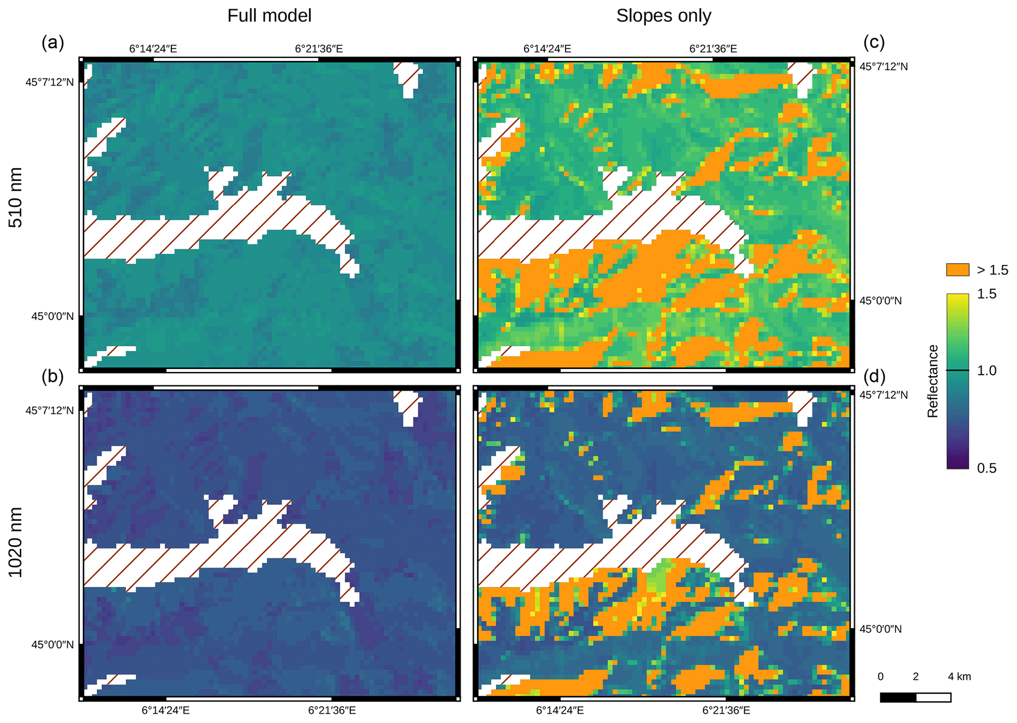
Figure 10Modelled surface reflectance using the full-rugged-terrain (a, b) and slope-only (c, d) formulations on 13 February 2018 at 510 nm (a, c) and 1020 nm (b, d). Pixels containing less than 80 % of snow were masked out (hatched region).
To infer surface geophysical properties from optical remote sensing data, it is common to first estimate surface reflectance by applying atmospheric corrections and second use the obtained surface reflectance spectra in subsequent retrieval algorithms. Here using REDRESS, the benefits of considering the full-rugged-terrain problem over simply accounting for slope effects on future BOA reflectance retrievals are evaluated. For this, the TOA radiance synthetic maps produced with REDRESS and REDRESSslope for the OLCI scene on 13 February 2018 were converted to BOA reflectance (Fig. 10). The synthetic BOA reflectance images are shown at 510 and 1020 nm, covering the study area delimited in Fig. 3. At both wavelengths, the images produced with REDRESS have relatively uniform values across the scene, with a mean value of 0.97 ± 0.03 (1σ) at 510 nm and 0.77 ± 0.03 (1σ) at 1020 nm. The BOA reflectance values vary across the image according to the slope and aspect of the terrain, with the DEM spatial signal clearly appearing. The model is able to simulate the reflectance in the shadowed areas well, although the variability is partly lost and thus reflectance appears as uniform patches in the shade. The images produced with REDRESSslope are more spatially variable (mean values of 1.45 ± 0.51, 1σ, and 1.39 ± 1.35, 1σ at 510 and 1020 nm, respectively). Furthermore, the BOA reflectance produced with REDRESSslope is systematically higher than with REDRESS, with average values at all wavelengths across the map being over 1. This overestimation is exacerbated in the shadowed areas of the image, where reflectance values are almost always over 1.5 at 510 nm (orange-shaded areas in Fig. 10), and for a large proportion at 1020 nm.
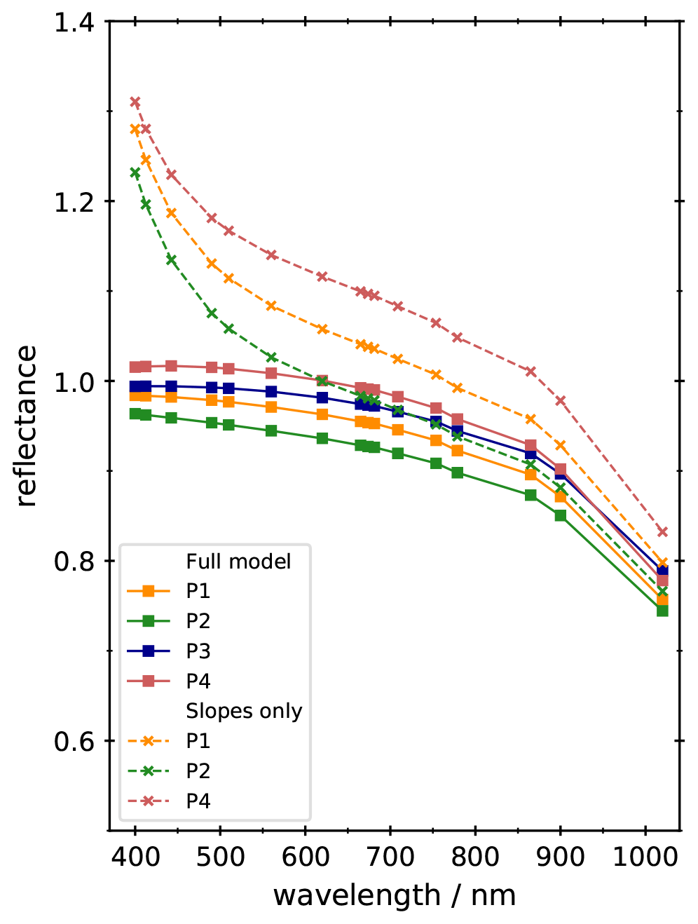
Figure 11Reflectance spectra simulated for 4 pixels (P1, P2, P3, and P4) across the study site on 13 February 2018 using REDRESS (solid lines) and REDRESSslope (dashed lines). The spectrum simulated for P3 with REDRESSslope is not shown here.
Examples of the BOA reflectance spectra at all bands are shown in Fig. 11 for the 4 pixels across the study site (Table 2). The spectra simulated using REDRESS (solid lines and squares) show a similar spectral shape, typical of fresh snow, for the four sites with values varying between 0.96 (P2) and 1.01 (P4) at 400 nm and between 0.74 (P2) and 0.79 (P3) at 1020 nm. The small differences observed between the sites are explained by changes in illumination and viewing angles caused by the slope and aspect of the surface (Picard et al., 2020). Contrastingly, the BOA reflectance obtained with REDRESSslope feature a marked decreasing trend in the 400–620 nm range for the sunlit pixels P1, P2, and P4 (decrease between 0.19 and 0.23), which differs from the flat response obtained with REDRESS (decrease between 0.01 and 0.03). In the near infrared, the BOA reflectance obtained with REDRESSslope is closer to that of REDRESS with a difference between the simulation configurations of 0.04, 0.02, and 0.05 for pixels P1, P2, and P4, respectively. The spectrum simulated with the REDRESSslope configuration is not shown for pixel P3, since it is shadowed, leading to highly unrealistic values which are often masked out or ignored (Scambos et al., 2007; Crawford et al., 2013). Figures 10 and 11 suggest that considering the full effects of rugged terrain (Eq. 1) would noticeably improve the retrievals of snow physical properties in shadowed areas. Furthermore, although the simulated reflectance for sunlit slopes is similar in the infrared wavelengths whether the full-rugged-terrain effects or just the slopes are considered due to the small proportion of diffuse illumination at those wavelengths, Fig. 11 indicates that considering the full-rugged-terrain problem will significantly improve reflectance retrievals in the visible wavelengths.
5.2 Limitations and further improvements
Although REDRESS shows promising results for the simulation and then correction of satellite scenes over snow-covered surfaces with complex topographic features, a number of uncertainties are introduced into the product in the course of the process.
First, the accuracy of the topographic products depends on the DEM used as input. The artefacts found in terrain changes in the results (Figs. 5 and 6) in relationship with shadows and ridges confirm the finding of Lenot et al. (2009), in which retrievals over rugged terrain were shown to be mostly impacted by the coarse resolution of the DEMs typically used or the errors in the orthorectification between the DEM and the satellite image (Richter, 1998). Here, the observed errors along the ridges may be due to the resolution of the DEM (30 m) or a misrepresentation of the terrain, since the overall vertical accuracy has been estimated to be 10–25 m (ASTER GDEM Validation Team, 2009), which is significant for calculating topographic parameters. Furthermore, even in the case of an accurate DEM, the resolution of the DEM can introduce errors at the ridges due to a smoothing effect of the topography leading to an overestimation of the radiance. Olson et al. (2019) showed that the incident shortwave radiation is overestimated in mountainous regions as the resolution of the DEM becomes coarser. On the contrary, the distribution of the pixels for which the TOA radiance is largely underestimated by the model along the borders of the shadowed areas in the image suggests that the calculation of the shadow extent is overestimated in the model, with sunlit pixels falling into the shadows. However, using DEM products with a higher resolution than the satellite image, as is recommended by Richter (1998), who suggests using a DEM with a resolution of 0.25 times the satellite image size, also introduces uncertainties into the calculation of topographic parameters that in turn affect the retrieval of snow properties. The use of high-resolution DEMs that are more and more accessible thanks to widespread high-resolution satellite imagery and airborne or drone-based platforms (e.g. Nolan et al., 2015; Bühler et al., 2016; Deschamps-Berger et al., 2020), does not necessarily improve the model's results. Indeed, as the resolution of the DEM increases compared to the satellite product, despite improvements in the estimation of illumination and viewing angles, the results become more sensitive to the sub-pixel heterogeneity. The higher-resolution products calculated from the DEM, including illumination and viewing geometries, need to be resampled to the coarser satellite pixel, causing a smoothing of angles. The BRDF of the snow surface that is calculated using these geometries may not be representative of the surface, as rougher surfaces tend to smooth out the BRDF effect (e.g Warren et al., 1998). Therefore, the BRDF model used in this study, which considers a smooth surface, will have a tendency to produce an excessively pronounced signal compared to the signal measured by the satellite. Further work on the accurate representation of the terrain at different spatial scales is recommended.
Second, the results in Fig. 9 also highlight how critical the atmospheric radiative-transfer calculations are at all wavelengths, the modelled TOA radiance having been shown here to be sensitive to the parameterisation of the atmosphere in the model. Figure 9 highlights the sensitivity of the TOA radiance to the AOD at 550 nm, even if the CAMS near-real-time product appears to have correctly evaluated the atmospheric parameters on the investigated dates. Nevertheless, small errors in the estimation of the AOD at the time of the satellite overpass may result in non-trivial errors in the retrieval of snow surface properties, with an overestimation of the AOD causing an overestimation of the radiance for sunlit pixels and an underestimation for shadowed pixels. The possibility of error is exacerbated by the fact that it is not uncommon to see changes in AOD by a factor of 3–5 from one day to another in the Alps (Lenoble et al., 2008). Additionally, the atmospheric radiative-transfer calculations consider clear skies only and do not account for cloud cover. Cloud-masking algorithms have been shown to perform badly over snow-covered terrain (Stillinger et al., 2019) and were not chosen to be applied to this work because the small extent of the studied area allowed visual selection of the images.
Third, in this study the TOA radiance is simulated with the same SSA across the scene, each scene having a different SSA, potentially introducing errors in the near infrared due to spatial variations in the surface snow properties. For the scene modelled on 13 February 2018, the assumption of uniform snow cover was reasonably valid as snowfall occurred less than 24 h before the satellite overpass. Despite these favourable conditions, a larger dispersion is obtained at 1020 nm (Fig. 6) compared to 510 nm (Fig. 5), suggesting possible uncertainties owing to surface property spatial variations. With the aim of using the model to retrieve surface parameters from satellite images, it will be possible to iteratively calculate and update the snow physical properties in every pixel. As well as considering a uniform SSA, the current application of REDRESS assumes 100 % snow cover, and snow-free pixels are removed a posteriori based on an external product. Therefore, errors in the snow cover product used to classify the pixels will result in large uncertainties in the model outputs, with an overestimation of the TOA radiance for pixels erroneously detected as snow-covered. To overcome the limitation, and for the large-scale application of REDRESS, further developments to iteratively estimate fractional snow cover derived from surface reflectance (Gascoin et al., 2019; Hall et al., 2002) are foreseen.
Further sources of uncertainty can be linked to the satellite sensor itself. Although Sentinel-3 OLCI has an onboard calibration assembly performing periodical radiometric calibrations, unaccounted for small changes in the stability of the sensors can occur. For example, it has been shown that Sentinel-3 OLCI overestimates radiance measurements over dark surfaces (Eumetsat, 2019). However, to the authors' knowledge no vicarious calibration studies have been performed over bright snow surfaces. Moreover, inter-sensor calibration differences should be kept in mind when processing data from multiple identical satellites such as the Sentinel fleets (Clerc et al., 2020). Lastly, drift in the calibration of the sensor over time may lead to changes in the acquired data that in turn could be misinterpreted as physical processes (e.g. Casey et al., 2017).
Although the calculation of the terms making up the TOA radiance over rugged terrain in REDRESS is computationally cheap, processing the topographic parameters used as inputs and running the Py6S radiative-transfer model considerably slow the process. The computational times were not of concern for the evaluation site selected in this study; nevertheless these two points are to be considered when running the model over larger areas such as an entire mountain range. First, the calculation of the horizons in 64 azimuth directions for each pixel (described in Sect. 3.1.4) is the most time-consuming process when running REDRESS, with an execution time of approximately 23 min for an image of 1000 pixels × 1000 pixels on a standard desktop computer (2 CPUs, 2.0 Ghz processor, 7.5 GB RAM). However, the model allows one to choose between calculating the horizon products as needed and using precalculated products. Thus for larger extents, the horizon products can be precalculated using the dedicated tool, a step that only needs to be performed once. Second, the model setup used in this study only performs the radiative-transfer calculations twice (Sect. 3.2.4) using averaged input values for the entire study area. The extent of the study area was considered sufficiently small for the differences in illumination and viewing geometries (typically < 0.5∘) as well as in atmospheric parameters to be negligible across the scene. However, for large study areas the radiative-transfer model needs to be run on a pixel-per-pixel basis to account for the sometimes large variations in the model inputs observed at a regional scale. This approach is not feasible with the current setup which takes approximately 2 s per pixel to compute the atmospheric parameters. Given the modular nature of REDRESS, the use of a radiative-transfer tool dedicated to satellite imagery correction or the adaptation of Py6S for use with precalculated lookup tables is recommended.
A new modular approach designed to simulate TOA radiance measured by space-borne optical sensors over snow-covered rugged terrain is presented. REDRESS, comprising a DEM-based forward model associated with a radiative-transfer model for the atmosphere and a dedicated snow BRDF model, allows one to estimate the different terms contributing to the measured signal and is adapted to account for highly reflective surfaces, for which scattering effects are exacerbated.
The model was applied to five Sentinel-3 OLCI scenes acquired over an entire winter season in the French Alps. For each date, REDRESS was initialised with snow SSA measurements performed in the area at the time of the satellite overpass and using the CAMS daily analysis of atmospheric conditions as input for the atmospheric radiative-transfer module. Results show that REDRESS is able to simulate TOA radiance images of snow-covered rugged terrain comparable to those measured by a multispectral optical space-borne sensor, as long as particular care is taken in the selection of the DEM and input source for the atmospheric parameters. Synthetic TOA images modelled using the full terrain problem show higher levels of agreement with the Sentinel-3 OLCI scenes compared to images simulated considering the effects of slopes only, particularly in shadowed areas or steep slopes. Furthermore, the study highlights the large variations in the terms making up the total TOA radiance in rugged terrain. Over the winter season (February–April 2018), the contribution to the total TOA signal of the radiation reflected from surrounding slopes towards observed sunlit pixels was in the range of 6 %–10 % and the diffuse contribution of multiple reflections from the neighbourhood coupled with the atmosphere represented 0.5 %–7 % of the signal, both with a larger contribution in the visible wavelengths. In the shadowed areas, the diffuse contribution of the neighbourhood was similar to that of the sunlit pixels. The contribution of surrounding slopes to the pixel's radiance was similar to the sunlit pixels in the visible wavelengths (6 %–8 %) but significantly larger in the near infrared, ranging from 8 % to 40 % across the season, owing to the other diffuse contributions being small. Because the reflected signal is weak in the near infrared, the neighbourhood contributions make up a larger proportion of the signal. The analysis of the different terms contributing to the TOA radiance has shown that the contributions of surrounding terrain cannot be neglected in the visible wavelengths even for small slopes (< 10∘) and have an important effect in shadowed areas in the infrared wavelengths. Accounting for the full-rugged-terrain problem is thus essential for optical satellite remote sensing observations over snow-covered mountainous terrain.
The source code of the REDRESS model, its documentation, and examples are available at the following GitHub repository: https://github.com/maximlamare/REDRESS (Lamare, 2020).
Sentinel-3A OLCI scenes were sourced as open data from the European Space Agency (ESA) Copernicus Open Access Hub (https://scihub.copernicus.eu/dhus/, European Space Agency, 2020). The SPOT 6 image was obtained via the CNES Kalideos Alpes project (https://alpes.kalideos.fr, Centre national d'études spatiales & Noveltis Kalideos Alpes, 2020). The atmospheric CAMS data were obtained via the ECMWF catalogue (https://www.ecmwf.int/, ECMWF, 2020). The Sentinel-2 snow cover data were sourced from the Theia platform (https://www.theia-land.fr/product/neige/, Pôle de données et de services surfaces continentales Theias, 2020).
ML, MD, and GP designed the study and developed the theory. ML, CD, FT, FL, and LA contributed to the acquisition of the field data. ML led the analysis and wrote the manuscript. All authors contributed to revisions of the manuscript.
The authors declare that they have no conflict of interest.
CNRM CEN and IGE are part of Labex OSUG@2020 (investissement d'avenir – ANR10 LABX56). This work has been carried out using the resources made available by the Copernicus Research and User Support (RUS) service (http://rus-copernicus.eu, last access: 12 November 2020), funded by the European Commission, managed by the European Space Agency, and operated by CS SI and its partners. The authors are grateful to Lautaret staff and staff at Station Alpine Joseph Fourier (SAJF) for instrument maintenance and for supporting the in situ experiments.
This research has been supported by the Agence Nationale de la Recherche (grant no. EBONI ANR-16-CE01-006), the Centre National d'Etudes Spatiales (APR CNES MIOSOTIS grant), and the Fondation BNP Paribas (APT project).
This paper was edited by Chris Derksen and reviewed by Jeff Dozier and one anonymous referee.
Arnaud, L., Picard, G., Champollion, N., Domine, F., Gallet, J., Lefebvre, E., Fily, M., and Barnola, J.: Measurement of vertical profiles of snow specific surface area with a 1 cm resolution using infrared reflectance: instrument description and validation, J. Glaciol., 57, 17–29, https://doi.org/10.3189/002214311795306664, 2011. a
ASTER GDEM Validation Team: ASTER Global DEM Validation Summary Report, meti & nasa edn., available at: https://lpdaac.usgs.gov/documents/28/ASTER_GDEM_Validation_1_Summary_Report.pdf (last access: 12 November 2020), 2009. a
Barnett, T. P., Adam, J. C., and Lettenmaier, D. P.: Potential impacts of a warming climate on water availability in snow-dominated regions, Nature, 438, 303–309, https://doi.org/10.1038/nature04141, 2005. a
Brun, F., Dumont, M., Wagnon, P., Berthier, E., Azam, M. F., Shea, J. M., Sirguey, P., Rabatel, A., and Ramanathan, Al.: Seasonal changes in surface albedo of Himalayan glaciers from MODIS data and links with the annual mass balance, The Cryosphere, 9, 341–355, https://doi.org/10.5194/tc-9-341-2015, 2015. a
Bühler, Y., Meier, L., and Ginzler, C.: Potential of Operational High Spatial Resolution Near-Infrared Remote Sensing Instruments for Snow Surface Type Mapping, IEEE Geosci. Remote S., 12, 821–825, https://doi.org/10.1109/LGRS.2014.2363237, 2015. a
Bühler, Y., Adams, M. S., Bösch, R., and Stoffel, A.: Mapping snow depth in alpine terrain with unmanned aerial systems (UASs): potential and limitations, The Cryosphere, 10, 1075–1088, https://doi.org/10.5194/tc-10-1075-2016, 2016. a
Campagnolo, M. L., Sun, Q., Liu, Y., Schaaf, C., Wang, Z., and Román, M. O.: Estimating the effective spatial resolution of the operational BRDF, albedo, and nadir reflectance products from MODIS and VIIRS, Remote Sens. Environ., 175, 52–64, https://doi.org/10.1016/J.RSE.2015.12.033, 2016. a
Centre national d'études spatiales & Noveltis Kalideos Alpes: Risques Gravitaires, Cryosphère et Végetation en zones alpines vus de l’espace, available at: https://alpes.kalideos.fr/, last access: 12 November 2020. a
Chappuis, J.: Sur le spectre d'absorption de l'ozone, C.R. Acad. Sci. Paris 91, 985–986, 1880. a
Civco, D. L.: Topographic Normalization of Landsat Thematic Mapper Digital Imagery, Photogramm. Eng. Rem. S., 55, 1303–1309, 1989. a
Cohen, J.: Snow cover and climate, Weather, 49, 150–156, https://doi.org/10.1002/j.1477-8696.1994.tb05997.x, 1994. a
Colby, J. D.: Topographic normalization in rugged terrain, in: Photogramm. Eng. Rem. S., 57, 531–537, 1991. a
Conese, C., Gilabert, M. A., Maselli, F., and Bottai, L.: Topographic Normalization of Tm Scenes Through the Use of an Atmospheric Correction Method and Digital Terrain Models, Photogramm. Eng. Rem. S., 59, 1745–1753, 1993a. a
Conese, C., Maracchi, G., and Maselli, F.: Improvement in Maximum Likelihood Classification performance on highly rugged terrain using Principal Components Analysis, Int. J. Remote Sens., 14, 1371–1382, https://doi.org/10.1080/01431169308953963, 1993b. a
Crawford, C. J., Manson, S. M., Bauer, M. E., and Hall, D. K.: Multitemporal snow cover mapping in mountainous terrain for Landsat climate data record development, Remote Sens. Environ., 135, 224–233, https://doi.org/10.1016/j.rse.2013.04.004, 2013. a
Deschamps-Berger, C., Gascoin, S., Berthier, E., Deems, J., Gutmann, E., Dehecq, A., Shean, D., and Dumont, M.: Snow depth mapping from stereo satellite imagery in mountainous terrain: evaluation using airborne laser-scanning data, The Cryosphere, 14, 2925–2940, https://doi.org/10.5194/tc-14-2925-2020, 2020. a
Dietz, A. J., Kuenzer, C., Gessner, U., and Dech, S.: Remote sensing of snow – a review of available methods, Int. J. Remote Sens., 33, 4094–4134, https://doi.org/10.1080/01431161.2011.640964, 2012. a
Dorren, L. K., Maier, B., and Seijmonsbergen, A. C.: Improved Landsat-based forest mapping in steep mountainous terrain using object-based classification, Forest Ecol. Manag., 183, 31–46, https://doi.org/10.1016/S0378-1127(03)00113-0, 2003. a
Dozier, J.: A clear-sky spectral solar radiation model for snow-covered mountainous terrain, Water Resour. Res., 16, 709–718, https://doi.org/10.1029/WR016i004p00709, 1980. a
Dozier, J.: Snow Reflectance from LANDSAT-4 Thematic Mapper, IEEE T. Geosci. Remote, GE-22, 323–328, https://doi.org/10.1109/TGRS.1984.350628, 1984. a
Dozier, J.: Spectral signature of alpine snow cover from the landsat thematic mapper, Remote Sens. Environ., 28, 9–22, https://doi.org/10.1016/0034-4257(89)90101-6, 1989. a, b
Dozier, J. and Frew, J.: Rapid calculation of terrain parameters for radiation modeling from digital elevation data, IEEE T. Geosci. Remote, 28, 963–969, https://doi.org/10.1109/36.58986, 1990. a, b
Dozier, J. and Painter, T. H.: Multispectral and Hyperspectral Remote Sensing of Alpine Snow Properties, Annu. Rev. Earth Pl. Sc., 32, 465–494, https://doi.org/10.1146/annurev.earth.32.101802.120404, 2004. a
Dozier, J., Bruno, J., and Downey, P.: A faster solution to the horizon problem, Comput. Geosci., 7, 145–151, https://doi.org/10.1016/0098-3004(81)90026-1, 1981. a, b
Dubayah, R. and Rich, P. M.: Topographic solar radiation models for GIS, Int. J. Geogr. Inf. Syst., 9, 405–419, https://doi.org/10.1080/02693799508902046, 1995. a, b
Duguay, C. and Ledrew, E.: Estimating surface reflectance and albedo from Landsat-5 Thematic Mapper over rugged terrain, Photogramm. Eng. Rem. S., 58, 551–558, 1992. a
Dumont, M., Sirguey, P., Arnaud, Y., and Six, D.: Monitoring spatial and temporal variations of surface albedo on Saint Sorlin Glacier (French Alps) using terrestrial photography, The Cryosphere, 5, 759–771, https://doi.org/10.5194/tc-5-759-2011, 2011. a, b
Dumont, M., Durand, Y., Arnaud, Y., and Six, D.: Variational assimilation of albedo in a snowpack model and reconstruction of the spatial mass-balance distribution of an alpine glacier, J. Glaciol., 58, 151–164, https://doi.org/10.3189/2012jog11j163, 2012a. a
Dumont, M., Gardelle, J., Sirguey, P., Guillot, A., Six, D., Rabatel, A., and Arnaud, Y.: Linking glacier annual mass balance and glacier albedo retrieved from MODIS data, The Cryosphere, 6, 1527–1539, https://doi.org/10.5194/tc-6-1527-2012, 2012b. a, b
Dumont, M., Arnaud, L., Picard, G., Libois, Q., Lejeune, Y., Nabat, P., Voisin, D., and Morin, S.: In situ continuous visible and near-infrared spectroscopy of an alpine snowpack, The Cryosphere, 11, 1091–1110, https://doi.org/10.5194/tc-11-1091-2017, 2017. a
European Centre for Medium-Range Weather Forecasts: ECMWF catalogue, available at: https://www.ecmwf.int/, last access: 12 November 2020. a
European Space Agency: Copernicus Open Access Hub, available at: https://scihub.copernicus.eu/dhus/, last access: 12 November 2020. a
Fily, M., Bourdelles, B., Dedieu, J., and Sergent, C.: Comparison of in situ and Landsat Thematic Mapper derived snow grain characteristics in the alps, Remote Sens. Environ., 59, 452–460, https://doi.org/10.1016/S0034-4257(96)00113-7, 1997. a
Flanner, M. G., Shell, K. M., Barlage, M., Perovich, D. K., and Tschudi, M. A.: Radiative forcing and albedo feedback from the Northern Hemisphere cryosphere between 1979 and 2008, Nat. Geosci., 4, 151–155, https://doi.org/10.1038/ngeo1062, 2011. a
Frey, H. and Paul, F.: On the suitability of the SRTM DEM and ASTER GDEM for the compilation of: Topographic parameters in glacier inventories, Int. J. Appl. Earth Obs., 18, 480–490, https://doi.org/10.1016/j.jag.2011.09.020, 2012. a
Gascoin, S., Grizonnet, M., Bouchet, M., Salgues, G., and Hagolle, O.: Theia Snow collection: high-resolution operational snow cover maps from Sentinel-2 and Landsat-8 data, Earth Syst. Sci. Data, 11, 493–514, https://doi.org/10.5194/essd-11-493-2019, 2019. a, b
Gastellu-Etchegorry, J. P., Martin, E., and Gascon, F.: DART: a 3D model for simulating satellite images and studying surface radiation budget, Int. J. Remote Sens., 25, 73–96, https://doi.org/10.1080/0143116031000115166, 2004. a
GDAL/OGR contributors: GDAL/OGR Geospatial Data Abstraction software Library, Open Source Geospatial Foundation, available at: https://gdal.org (last access: 12 November 2020), 2019. a
Guyomarc'h, G., Bellot, H., Vionnet, V., Naaim-Bouvet, F., Déliot, Y., Fontaine, F., Puglièse, P., Nishimura, K., Durand, Y., and Naaim, M.: A meteorological and blowing snow data set (2000–2016) from a high-elevation alpine site (Col du Lac Blanc, France, 2720 ), Earth Syst. Sci. Data, 11, 57–69, https://doi.org/10.5194/essd-11-57-2019, 2019. a
Hall, D. K., Riggs, G. A., Salomonson, V. V., DiGirolamo, N. E., and Bayr, K. J.: MODIS snow-cover products, Remote Sens. Environ., 83, 181–194, https://doi.org/10.1016/S0034-4257(02)00095-0, 2002. a
Holben, B. and Justice, C.: An examination of spectral band ratioing to reduce the topographic effect on remotely sensed data, Int. J. Remote Sens., 2, 115–133, https://doi.org/10.1080/01431168108948349, 1981. a
Holben, B. N. and Justice, C. .O: The Topographic Effect on Spectral Response from Nadir-Pointing Sensors, Photogramm. Eng. Rem. S., 46, 1191–1200, 1980. a
Horn, B.: Hill shading and the reflectance map, P. IEEE, 69, 14–47, https://doi.org/10.1109/PROC.1981.11918, 1981. a
Jamieson, B. and Stethem, C.: Snow Avalanche Hazards and Management in Canada: Challenges and Progress, Nat. Hazards, 26, 35–53, https://doi.org/10.1023/A:1015212626232, 2002. a
Klein, A. G. and Stroeve, J.: Development and validation of a snow albedo algorithm for the MODIS instrument, Ann. Glaciol., 34, 45–52, https://doi.org/10.3189/172756402781817662, 2002. a, b
Kokhanovsky, A., Lamare, M., Danne, O., Brockmann, C., Dumont, M., Picard, G., Arnaud, L., Favier, V., Jourdain, B., Le Meur, E., Di Mauro, B., Aoki, T., Niwano, M., Rozanov, V., Korkin, S., Kipfstuhl, S., Freitag, J., Hoerhold, M., Zuhr, A., Vladimirova, D., Faber, A.-K., Steen-Larsen, H. C., Wahl, S., Andersen, J. K., Vandecrux, B., van As, D., Mankoff, K. D., Kern, M., Zege, E., and Box, J. E.: Retrieval of Snow Properties from the Sentinel-3 Ocean and Land Colour Instrument, Remote Sens.-Basel, 11, https://doi.org/10.3390/rs11192280, 2019. a
Kokhanovsky, A. A. and Breon, F. M.: Validation of an analytical snow BRDF model using PARASOL multi-angular and multispectral observations, IEEE Geosci. Remote S., 9, 928–932, https://doi.org/10.1109/LGRS.2012.2185775, 2012. a, b
Kokhanovsky, A. A. and Schreier, M.: The determination of snow albedo using combined aatsr and meris observations, European Space Agency, (Special Publication) ESA SP, 2008. a
Kokhanovsky, A. A. and Zege, E. P.: Scattering optics of snow, Appl. Optics, 43, 1589–1602, https://doi.org/10.1364/AO.43.001589, 2004. a, b, c
König, M., Winther, J.-G., and Isaksson, E.: Measuring snow and glacier ice properties from satellite, Rev. Geophys., 39, 1–27, https://doi.org/10.1029/1999RG000076, 2001. a
Lamare, M.: REDRESS GitHub repository, GitHub, available at: https://github.com/maximlamare/REDRESS, last access: 12 November 2020. a
Larue, F., Picard, G., Arnaud, L., Ollivier, I., Delcourt, C., Lamare, M., Tuzet, F., Revuelto, J., and Dumont, M.: Snow albedo sensitivity to macroscopic surface roughness using a new ray-tracing model, The Cryosphere, 14, 1651–1672, https://doi.org/10.5194/tc-14-1651-2020, 2020. a
Lee, S. and Clarke, K.: An assessment of differences in algorithms for computing fundamental topographic parameters, AutoCarto Proceedings Papers, available at: https://cartogis.org/docs/proceedings/2005/lee_clark.pdf (last access: 12 November 2020), 2005. a
Lenoble, J., Brogniez, C., de La Casinière, A., Cabot, T., Buchard, V., and Guirado, F.: Measurements of UV aerosol optical depth in the French Southern Alps, Atmos. Chem. Phys., 8, 6597–6602, https://doi.org/10.5194/acp-8-6597-2008, 2008. a
Lenot, X., Achard, V., and Poutier, L.: SIERRA: A new approach to atmospheric and topographic corrections for hyperspectral imagery, Remote Sens. Environ., 113, 1664–1677, https://doi.org/10.1016/J.RSE.2009.03.016, 2009. a, b, c, d, e, f, g, h, i, j
Leprieur, J., Durand, C., and Peyron, J.: Influence of topography on forest reflectance using Landsat Thematic Mapper and digital terrain data, Photogramm. Eng. Rem. S., 54, 491–496, 1988. a
Li, X., Cheng, G., Chen, X., and Lu, L.: Modification of solar radiation model over rugged terrain, Chinese Sci. Bull., 44, 1345–1349, https://doi.org/10.1007/BF02885977, 1999. a
Lonjou, V., Desjardins, C., Hagolle, O., Petrucci, B., Tremas, T., Dejus, M., Makarau, A., and Auer, S.: MACCS-ATCOR joint algorithm (MAJA), in: Remote Sensing of Clouds and the Atmosphere XXI, vol. 10001, Proc. SPIE, 10001, https://doi.org/10.1117/12.2240935, 2016. a
Maignan, F., Bréon, F.-M., and Lacaze, R.: Bidirectional reflectance of Earth targets: evaluation of analytical models using a large set of spaceborne measurements with emphasis on the Hot Spot, Remote Sens. Environ., 90, 210–220, https://doi.org/10.1016/j.rse.2003.12.006, 2004. a
Main-Knorn, M., Pflug, B., Louis, J., Debaecker, V., Müller-Wilm, U., and Gascon, F.: Sen2Cor for Sentinel-2, in: Image and Signal Processing for Remote Sensing XXIII, vol. 10427, Proc. SPIE, 10427, https://doi.org/10.1117/12.2278218, 2017. a
Malcher, P., Floricioiu, D., and Rott, H.: Snow mapping in Alpine areas using medium resolution spectrometric sensors, in: IGARSS 2003, 2003 IEEE International Geoscience and Remote Sensing Symposium, Proceedings (IEEE Cat. No.03CH37477), vol. 4, IEEE, https://doi.org/10.1109/IGARSS.2003.1294603, 2835–2837, 2003. a
Masson, T., Dumont, M., Mura, M. D., Sirguey, P., Gascoin, S., Dedieu, J.-P., and Chanussot, J.: An Assessment of Existing Methodologies to Retrieve Snow Cover Fraction from MODIS Data, Remote Sens.-Basel, 10, 619, https://doi.org/10.3390/rs10040619, 2018. a
Mayer, B., Hoch, S. W., and Whiteman, C. D.: Validating the MYSTIC three-dimensional radiative transfer model with observations from the complex topography of Arizona's Meteor Crater, Atmos. Chem. Phys., 10, 8685–8696, https://doi.org/10.5194/acp-10-8685-2010, 2010. a
Mishra, V., Sharma, J., and Khanna, R.: Review of topographic analysis methods for the western Himalaya using AWiFS and MODIS satellite imagery, Ann. Glaciol., 51, 153–160, https://doi.org/10.3189/172756410791386526, 2010. a
Mousivand, A., Verhoef, W., Menenti, M., and Gorte, B.: Modeling Top of Atmosphere Radiance over Heterogeneous Non-Lambertian Rugged Terrain, Remote Sens.-Basel, 7, 8019–8044, https://doi.org/10.3390/rs70608019, 2015. a
NASA/METI/AIST/U.S. & Japan Spacesystems: ASTER Global Digital Elevation Model V003 [Data set], NASA EOSDI edn., https://doi.org/10.5067/ASTER/ASTGTM.003, 2019. a
Neckel, H. and Labs, D.: The solar radiation between 3300 and 12 500 Å, Sol. Phys., 90, 205–258, 1984. a
Negi, H. S. and Kokhanovsky, A.: Retrieval of snow grain size and albedo of western Himalayan snow cover using satellite data, The Cryosphere, 5, 831–847, https://doi.org/10.5194/tc-5-831-2011, 2011. a
Nolan, M., Larsen, C., and Sturm, M.: Mapping snow depth from manned aircraft on landscape scales at centimeter resolution using structure-from-motion photogrammetry, The Cryosphere, 9, 1445–1463, https://doi.org/10.5194/tc-9-1445-2015, 2015. a
Nolin, A. W.: Recent advances in remote sensing of seasonal snow, J. Glaciol., 56, 1141–1150, https://doi.org/10.3189/002214311796406077, 2010. a
Olson, M., Rupper, S., and Shean, D. E.: Terrain Induced Biases in Clear-Sky Shortwave Radiation Due to Digital Elevation Model Resolution for Glaciers in Complex Terrain, Front. Earth Sci., 7, 216, https://doi.org/10.3389/feart.2019.00216, 2019. a
Painter, T. H., Rittger, K., McKenzie, C., Slaughter, P., Davis, R. E., and Dozier, J.: Retrieval of subpixel snow covered area, grain size, and albedo from MODIS, Remote Sens. Environ., 113, 868–879, https://doi.org/10.1016/j.rse.2009.01.001, 2009. a
Picard, G., Dumont, M., Lamare, M., Tuzet, F., Larue, F., Pirazzini, R., and Arnaud, L.: Spectral albedo measurements over snow-covered slopes: theory and slope effect corrections, The Cryosphere, 14, 1497–1517, https://doi.org/10.5194/tc-14-1497-2020, 2020. a, b
Poglio, T., Mathieu-Marni, S., Ranchin, T., Savaria, E., and Wald, L.: OSIrIS: a physically based simulation tool to improve training in thermal infrared remote sensing over urban areas at high spatial resolution, Remote Sens. Environ., 104, 238–246, https://doi.org/10.1016/j.rse.2006.03.017, 2006. a
Pôle de données et de services surfaces continentales Theias: Theia Neige, available at: https://www.theia-land.fr/product/neige/, last access: 12 November 2020. a
Proy, C., Tanré, D., and Deschamps, P.: Evaluation of topographic effects in remotely sensed data, Remote Sens. Environ., 30, 21–32, https://doi.org/10.1016/0034-4257(89)90044-8, 1989. a, b
Qu, X. and Hall, A.: Assessing Snow Albedo Feedback in Simulated Climate Change, J. Climate, 19, 2617–2630, https://doi.org/10.1175/JCLI3750.1, 2006. a
Qu, Y., Liu, Q., Liang, S., Wang, L., Liu, N., and Liu, S.: Direct-Estimation Algorithm for Mapping Daily Land-Surface Broadband Albedo From MODIS Data, IEEE T. Geosci. Remote, 52, 907–919, https://doi.org/10.1109/TGRS.2013.2245670, 2014. a
Rahman, H., Pinty, B., and Verstraete, M. M.: Coupled surface-atmosphere reflectance (CSAR) model: 2. Semiempirical surface model usable with NOAA advanced very high resolution radiometer data, J. Geophys. Res.-Atmos., 98, 20791–20801, https://doi.org/10.1029/93JD02072, 1993. a
Richter, R.: Correction of atmospheric and topographic effects for high spatial resolution satellite imagery, Int. J. Remote Sens., 18, 1099–1111, https://doi.org/10.1080/014311697218593, 1997. a
Richter, R.: Correction of satellite imagery over mountainous terrain, Appl. Optics, 37, 4004, https://doi.org/10.1364/ao.37.004004, 1998. a, b, c, d, e, f, g
Richter, R. and Schläpfer, D.: Geo-atmospheric processing of airborne imaging spectrometry data. Part 2: Atmospheric/topographic correction, Int. J. Remote Sens., 23, 2631–2649, https://doi.org/10.1080/01431160110115834, 2002. a
Sandmeier, S. and Itten, K.: A physically-based model to correct atmospheric and illumination effects in optical satellite data of rugged terrain, IEEE T. Geosci. Remote, 35, 708–717, https://doi.org/10.1109/36.581991, 1997. a, b
Scambos, T. A., Haran, T. M., Fahnestock, M. A., Painter, T. H., and Bohlander, J.: MODIS-based Mosaic of Antarctica (MOA) data sets: Continent-wide surface morphology and snow grain size, Remote Sens. Environ., 111, 242–257, https://doi.org/10.1016/j.rse.2006.12.020, 2007. a, b
Schaaf, C. B., Gao, F., Strahler, A. H., Lucht, W., Li, X., Tsang, T., Strugnell, N. C., Zhang, X., Jin, Y., Muller, J. P., Lewis, P., Barnsley, M., Hobson, P., Disney, M., Roberts, G., Dunderdale, M., Doll, C., D'Entremont, R. P., Hu, B., Liang, S., Privette, J. L., and Roy, D.: First operational BRDF, albedo nadir reflectance products from MODIS, Remote Sens. Environ., 83, 135–148, https://doi.org/10.1016/S0034-4257(02)00091-3, 2002. a
Schaepman-Strub, G., Schaepman, M., Painter, T., Dangel, S., and Martonchik, J.: Reflectance quantities in optical remote sensing–definitions and case studies, Remote Sens. Environ., 103, 27–42, https://doi.org/10.1016/J.RSE.2006.03.002, 2006. a, b, c, d
Schlapfer, D., Richter, R., and Feingersh, T.: Operational BRDF effects correction for wide-field-of-view optical scanners (BREFCOR), IEEE T. Geosci. Remote, 53, 1855–1864, https://doi.org/10.1109/TGRS.2014.2349946, 2015. a, b
Sirguey, P.: Simple correction of multiple reflection effects in rugged terrain, Int. J. Remote Sens., 30, 1075–1081, https://doi.org/10.1080/01431160802348101, 2009. a, b
Sirguey, P., Mathieu, R., and Arnaud, Y.: Subpixel monitoring of the seasonal snow cover with MODIS at 250 m spatial resolution in the Southern Alps of New Zealand: Methodology and accuracy assessment, Remote Sens. Environ., 113, 160–181, https://doi.org/10.1016/J.RSE.2008.09.008, 2009. a, b, c, d, e, f, g, h, i, j, k, l, m
Sirguey, P., Still, H., Cullen, N. J., Dumont, M., Arnaud, Y., and Conway, J. P.: Reconstructing the mass balance of Brewster Glacier, New Zealand, using MODIS-derived glacier-wide albedo, The Cryosphere, 10, 2465–2484, https://doi.org/10.5194/tc-10-2465-2016, 2016. a
Sjoberg, R. W. and Horn, B. K. P.: Atmospheric effects in satellite imaging of mountainous terrain, Appl. Optics, 22, 1702, https://doi.org/10.1364/AO.22.001702, 1983. a
Stillinger, T., Roberts, D. A., Collar, N. M., and Dozier, J.: Cloud Masking for Landsat 8 and MODIS Terra Over Snow-Covered Terrain: Error Analysis and Spectral Similarity Between Snow and Cloud, Water Resour. Res., 55, 6169–6184, https://doi.org/10.1029/2019WR024932, 2019. a
Stroeve, J., Nolin, A., and Steffen, K.: Comparison of AVHRR-derived and in situ surface albedo over the greenland ice sheet, Remote Sens. Environ., 62, 262–276, https://doi.org/10.1016/S0034-4257(97)00107-7, 1997. a
Stroeve, J. C., Box, J. E., and Haran, T.: Evaluation of the MODIS (MOD10A1) daily snow albedo product over the Greenland ice sheet, Remote Sens. Environ., 105, 155–171, https://doi.org/10.1016/J.RSE.2006.06.009, 2006. a
Teillet, P., Guindon, B., and Goodenough, D.: On the Slope-Aspect Correction of Multispectral Scanner Data, Can. J. Remote Sens., 8, 84–106, https://doi.org/10.1080/07038992.1982.10855028, 1982. a, b
Trujillo, E., Molotch, N. P., Goulden, M. L., Kelly, A. E., and Bales, R. C.: Elevation-dependent influence of snow accumulation on forest greening, Nat. Geosci., 5, 705, https://doi.org/10.1038/ngeo1571, 2012. a
Vermote, E., Tanré, D., Deuzé, J. L., Herman, M., Morcrette, J. J., and Kotchenova, S. Y.: 6S User Guide Version 3, available at: http://6s.ltdri.org/pages/manual.html (last access: 12 November 2020), 2006. a
Vermote, E. F., Tanré, D., Deuzé, J. L., Herman, M., and Morcrette, J. J.: Second simulation of the satellite signal in the solar spectrum, 6s: an overview, IEEE T. Geosci. Remote, 35, 675–686, https://doi.org/10.1109/36.581987, 1997. a
Warren, S. G.: Optical properties of snow, Rev. Geophys., 20, 67–89, https://doi.org/10.1029/RG020i001p00067, 1982. a
Warren, S. G. and Wiscombe, W. J.: A Model for the Spectral Albedo of Snow. II: Snow Containing Atmospheric Aerosols, J. Atmos. Sci., 37, 2734–2745, https://doi.org/10.1175/1520-0469(1980)037<2734:AMFTSA>2.0.CO;2, 1980. a
Warren, S. G., Brandt, R. E., and O'Rawe Hinton, P.: Effect of surface roughness on bidirectional reflectance of Antarctic snow, J. Geophys. Res.-Planet., 103, 25789–25807, https://doi.org/10.1029/98JE01898, 1998. a
Williams, C. J., McNamara, J. P., and Chandler, D. G.: Controls on the temporal and spatial variability of soil moisture in a mountainous landscape: the signature of snow and complex terrain, Hydrol. Earth Syst. Sci., 13, 1325–1336, https://doi.org/10.5194/hess-13-1325-2009, 2009. a
Wilson, R. T.: Py6S: A Python interface to the 6S radiative transfer model., Comput. Geosci., 51, 166–171, https://doi.org/10.1016/j.cageo.2012.08.002, 2013. a
Woodham, R. and Gray, M.: An Analytic Method for Radiometric Correction of Satellite Multispectral Scanner Data, IEEE T. Geosci. Remote, GE-25, 258–271, https://doi.org/10.1109/TGRS.1987.289798, 1987. a
Xin, L., Koike, T., and Guodong, C.: Retrieval of snow reflectance from Landsat data in rugged terrain, Ann. Glaciol., 34, 31–37, https://doi.org/10.3189/172756402781817635, 2002. a
Yang, C. and Vidal, A.: Combination of digital elevation models with SPOT-1 HRV multispectral imagery for reflectance factor mapping, Remote Sens. Environ., 32, 35–45, https://doi.org/10.1016/0034-4257(90)90096-5, 1990. a