the Creative Commons Attribution 4.0 License.
the Creative Commons Attribution 4.0 License.
 | 13 Nov 2020
Numerical modeling of the dynamics of the Mer de Glace glacier, French Alps: comparison with past observations and forecasting of near-future evolution
Vincent Peyaud
Coline Bouchayer
Olivier Gagliardini
Christian Vincent
Fabien Gillet-Chaulet
Delphine Six
Olivier Laarman
Alpine glaciers are shrinking and rapidly loosing mass in a warming climate. Glacier modeling is required to assess the future consequences of these retreats on water resources, the hydropower industry and risk management. However, the performance of such ice flow modeling is generally difficult to evaluate because of the lack of long-term glaciological observations. Here, we assess the performance of the Elmer/Ice full Stokes ice flow model using the long dataset of mass balance, thickness change, ice flow velocity and snout fluctuation measurements obtained between 1979 and 2015 on the Mer de Glace glacier, France. Ice flow modeling results are compared in detail to comprehensive glaciological observations over 4 decades including both a period of glacier expansion preceding a long period of decay. To our knowledge, a comparison to data at this detail is unprecedented. We found that the model accurately reconstructs the velocity, elevation and length variations of this glacier despite some discrepancies that remain unexplained. The calibrated and validated model was then applied to simulate the future evolution of Mer de Glace from 2015 to 2050 using 26 different climate scenarios. Depending on the climate scenarios, the largest glacier in France, with a length of 20 km, could retreat by 2 to 6 km over the next 3 decades.
- Article
(16020 KB) - Full-text XML
-
Supplement
(1414 KB) - BibTeX
- EndNote


Mountain glacier mass balances show a strong sensitivity to climate change and can thus be used to assess the impact of climate change in remote areas (Oerlemans, 2001; Zemp et al., 2019). During the 20th century, all alpine glaciers showed a strong recession (Zemp et al., 2015). This observed trend is expected to continue in the future under a warming climate (IPCC, 2019) with important impacts on watershed hydrology (Huss and Hock, 2018; Brunner et al., 2019), tourism and hydropower resources (e.g., Welling et al., 2015; Stewart et al., 2016), accompanied by the emergence of new risks (e.g., Kääb et al., 2018) and sea-level rise (Hock et al., 2019; Marzeion et al., 2020). Properly assessing these future impacts requires the development of modeling tools capable of describing the processes driving these glacier changes.
Numerical ice flow models with different degrees of complexity have been developed to forecast glacier evolutions. The first studies of individual glaciers (e.g., Huybrechts et al., 1989; Letréguilly and Reynaud, 1989; Stroeven et al., 1989; Greuell, 1992) were constrained to flow line models related to the local driving stress, while studies on a regional scale (since Haeberli and Hölzle, 1995) focused on empirical approaches in which ice dynamics is not explicitly taken into account and glacier evolution is based on parameterizations calibrated with either equilibrium-line altitude (ELA) models (e.g., Zemp et al., 2006), extrapolations of observed geometry changes (e.g., Huss et al., 2008; Huss, 2012; Huss and Hock, 2018), or volume and length–area scalings (e.g., Marzeion et al., 2012; Radić et al., 2014). Process-based models were also developed to integrate simple dynamics (e.g., Le Meur and Vincent, 2003; Clarke et al., 2015; Zekollari et al., 2019; Maussion et al., 2019). These studies suggest a glacier volume loss from 65 % to 94 % in Central Europe by the end of the century depending on the climate scenario (IPCC, 2019; Marzeion et al., 2020). However, the Fourth Intergovernmental Panel on Climate Change (IPCC) Assessment Report (Solomon et al., 2007) and other studies (e.g., Vincent et al., 2014) emphasize the need for a new generation of glacier models that accurately describe the ice flow dynamics to correctly forecast individual glacier evolution. Today, such three-dimensional physical models are widely available. Indeed, with the improvement of computational resource performance, running a model describing the Stokes ice flow solution for the complex three-dimensional geometry of a whole glacier has become much more affordable (e.g., Réveillet et al., 2015; Jouvet and Huss, 2019; Gilbert et al., 2020). Among such models, Elmer/Ice (Gagliardini et al., 2013) has already been used for a number of glacier applications (e.g., Gagliardini et al., 2011; Réveillet et al., 2015; Gilbert et al., 2020) and will be used for this study.
However, very few glacier datasets are available to make a detailed comparison between observed and modeled fluctuations at the multi-decadal scale. Mer de Glace offers a rare opportunity to compare state-of-the-art model results with a large dataset containing observed thickness changes, ice flow velocities and snout fluctuations over a nearly continuous 40-year period thanks to the GLACIOCLIM observatory monitoring program (Vincent, 2002; Vincent et al., 2014; Berthier et al., 2004, 2005, 2014; Berthier and Vincent, 2012). In addition, running simulations on this glacier provides the opportunity to fulfill the need of capturing with a full Stokes ice flow model the local complex ice dynamics of a glacier that presented a large advance before the 1980s, followed by a rapid retreat over 3 decades.
In this paper, the performance of the Elmer/Ice ice flow model is first assessed in terms of its ability to reconstruct these past multi-decadal fluctuations in the tongue of Mer de Glace. A thorough comparison makes it possible to explore the sources of discrepancies between the reconstruction and the observations. In a second step, prognostic simulations are performed to simulate the evolution of the glacier until 2050 under different climate scenarios.
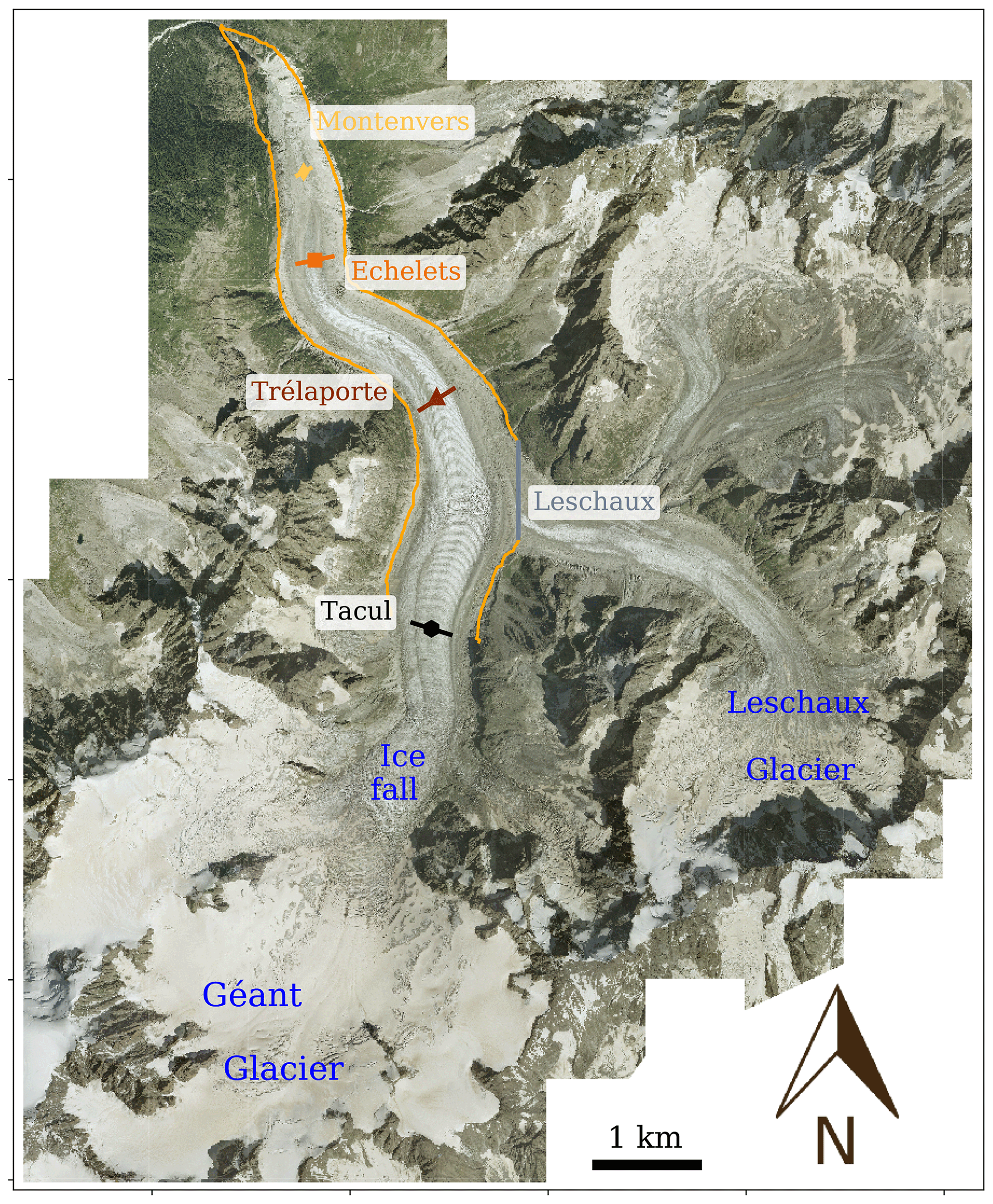
Figure 1Map of Mer de Glace (orthophoto acquired in 2008 ©RGD74). The orange contour delimits the area modeled in this study. The location of the four cross sections (Tacul, Trélaporte, Echelets and Montenvers) and the Leschaux gate are indicated by the colored lines. The Tacul and Leschaux gates represent boundary gates where data are used to force the model, whereas the three other profiles represent internal gates where data are used to validate the model.
Mer de Glace (45∘55′ N, 6∘57′ E) and the Géant glacier form the largest glacier in the French Alps which covers an area of 32 km2. It is located in the Mont Blanc massif (Fig. 1) and is monitored as part of the GLACIOCLIM observatory (https://glacioclim.osug.fr/, last access: 3 November 2020). The upper accumulation area, named Géant glacier, reaches 4300 m a.s.l. (above sea level). From this accumulation region, the ice flows at a speed of up to 500 m yr−1 (Millan et al., 2019) through a narrow, steep portion (an icefall between 2700 and 2400 m a.s.l.) before feeding Mer de Glace that covers the lower, 7 km long section above the terminus located at 1534 m a.s.l. in 2018. As shown in Fig. 1, Mer de Glace has a single tributary glacier which is named Leschaux glacier.
Several surface digital elevation models (DEMs) are available for different times in the past. The first map was produced in 1905 by Vallot (1905) using the classical topographic method. Another DEM was made by the Institut Géographique National (IGN) in 1979, and two were made by the Laboratory of Glaciology of Grenoble in 2003 and 2008 using aerial photographs (Vincent et al., 2014). A surface velocity field was derived from SPOT-5 (Système Probatoire d'Observation de la Terre) in 2003. Moreover, continuous field measurements have been performed at the lower part of the glacier (below 2300 m a.s.l.) from a network of stakes that have been monitored continuously since 1979 at four different elevations: the Tacul (2148 m a.s.l. in 2018), Trélaporte (1937 m a.s.l.), Echelets (1725 m a.s.l.) and Montenvers (1627 m a.s.l.) cross sections (see Fig. 1). Surface elevation has been measured systematically each year since 1979 along these four cross sections. Surface mass balance and annual surface velocity observations are also available at these cross sections, although they are not continuous between 1979 and 1994 except for observations at the Tacul cross section, which are continuous over the whole period. The bedrock topography was determined below 2300 m a.s.l. using mechanical borehole drillings, seismic soundings (Süustrunk, 1951; Vallon, 1961, 1967; Gluck, 1967) and radar measurements (2018; not published).
Given the lack of bedrock topography measurements in the upper part of the glacier (above the ice fall of Géant glacier) and the absence of measurements of bedrock topography for Leschaux glacier, the model domain was restricted to the lower part of the glacier from the Tacul cross section down to the snout. Here, we assume that the contribution of the Géant and Leschaux glaciers to Mer de Glace can be represented as specified flux conditions on the boundary of the Mer de Glace model.
3.1 Ice flow model
Mer de Glace ice flow dynamics are modeled with the Elmer/Ice open-source finite-element model (Gagliardini et al., 2013). This model has been applied to simulate real and artificial mountain glaciers (e.g., Farinotti et al., 2017; Gilbert et al., 2020).
The three-dimensional velocity field and p, the isotopic pressure, are solutions to the Stokes equations that express conservation of momentum and conservation of mass for an incompressible fluid. We use the viscous isotropic nonlinear Glen's law (Glen, 1955) to link the deviatoric-stress tensor to the strain-rate tensor. The Glen's exponent is n=3, and, assuming temperate ice, the rheological parameter A has a constant value (A=158 ; Paterson, 1994). Indeed, the ice of the lower part of Mer de Glace glacier is most likely temperate (Lliboutry et al., 1962).
The upper surface of the glacier is a free surface of elevation zs (m) that evolves with time according to the following kinematic equation:
where the surface mass balance b(z,t), in ice equivalent thickness (m yr−1), is a function of surface elevation and time, and denotes the surface velocity vector. As the finite element mesh cannot have a null thickness, a lower limit of 1 m above the bedrock elevation is applied to zs in Eq. (1).
3.2 Boundary conditions
Three types of boundary conditions are applied at the base, on the upper surface and on the two upstream gates of Tacul and Leschaux.
On the lower surface, a basal sliding is applied, as described in Sect. 3.2.1. On the upper surface, the surface mass balance (SMB) required in the free surface equation (Eq. 1) is derived either from observations when available or based on a positive degree day (PDD) model forced by climate simulations for the future. The two methods are explained in detail in Sect. 3.2.2.
The model domain does not cover the whole glacial catchment (see Fig. 1). Measurements of the bed are very sparse upstream of the Tacul gate and nonexistent on the Leschaux glacier. Modeling the whole glacier with a simple interpolation or a reconstructed bedrock would introduce large uncertainties. The large dataset of observations of thickness and centerline velocity collected at the Tacul cross section allows a good constraint on the flux passing through the gate. Observations at Leschaux cross section are limited, but, as presented in Sect. 3.2.3, the ice flow is much lower and has therefore a lower influence on the glacier evolution. Thus, in this study, the evolution of Mer de Glace is driven by two flux boundary conditions applied at the Tacul and Leschaux gates that prescribe the ice flux from the upstream accumulation areas of the glacier. The flux coming from the upper part of the glacier through the Tacul gate boundary condition is imposed from observations (thickness and central horizontal velocity at the Tacul gate) from the past and the estimated flux in the future. A similar method based on a flux is applied at the junction with Leschaux glacier. The implementation of an ice flux at these two gates for hindcast and forecast simulations differs slightly and is described in detail in Sect. 3.2.3.
Our simulations cover the period 1979–2050. The hindcast simulation covers the period 1979–2015 for which surface mass balances, surface velocities and elevation changes are available yearly at the four cross sections of Tacul, Trélaporte, Echelets and Montenvers (Fig. 1). The dataset at the Tacul cross section is used to specify the flux on this artificial boundary of the glacier domain, while the three others are used to evaluate the model over the hindcast period. For the forecast simulations from 2015 until 2050, results from climate simulations are used to simulate the future flux evolution at the boundary of the glacier domain.
Sections 3.2.2 and 3.2.3 describe in detail the respective boundary conditions for the two steps (hindcast and forecast) defined at the surface (mass balance) and at the Tacul and Leschaux gates (ice flux from the accumulation areas), respectively.
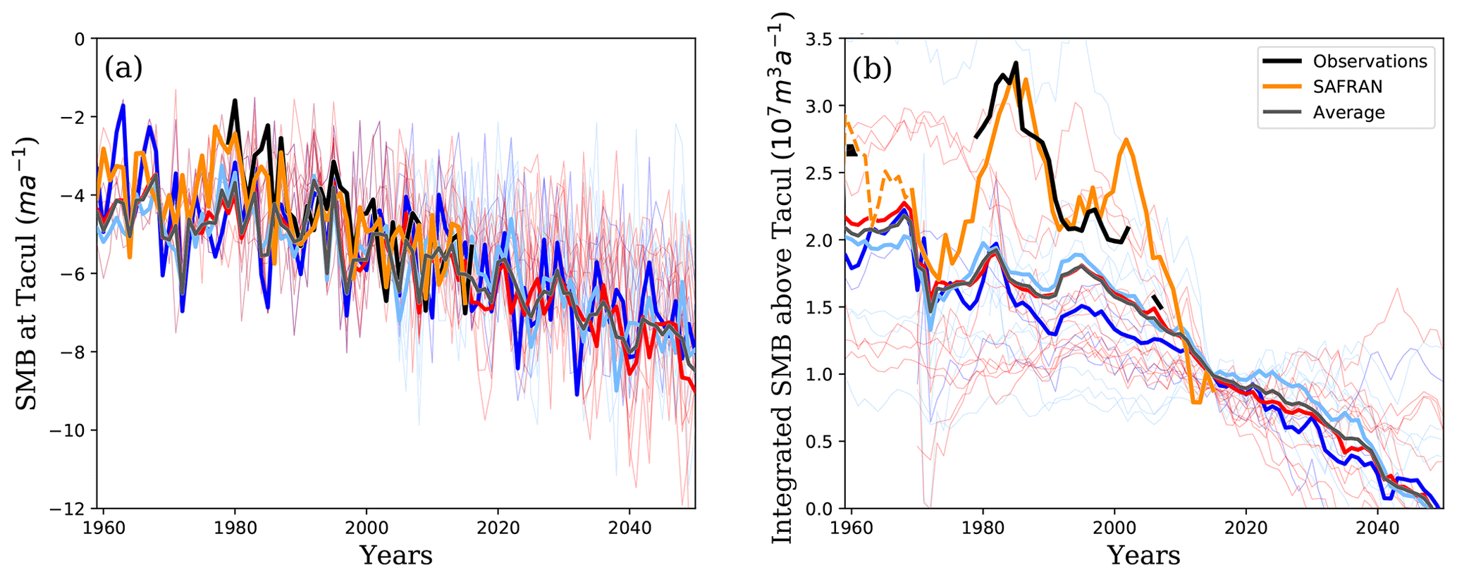
Figure 2Evolution with time from 1960 to 2050 of (a) the surface mass balances (SMBs) at the Tacul gate and (b) the integrated surface mass balance above the Tacul gate. Observations are presented in black and values inferred from SAFRAN in orange. The others climate scenarios are plotted in dark blue (RCP 2.6), blue (RCP 4.5) and red (RCP 8.5); the average values for each scenario are highlighted by thick curves. Note that for the past period 1960–2015, the integrated surface mass balance above the Tacul gate in (b) does correspond to the flux at this gate and that “observations” are not from direct observations but are actually estimated from surface velocity and elevation following the method used in Berthier and Vincent (2012). All integrated surface mass balances for the forecast simulations are normalized to the 2015 observed mass balance.
3.2.1 Basal conditions
At the base, ice cannot penetrate into the bed so the velocity component normal to the bed is null. As Mer de Glace is a temperate glacier, a certain amount of sliding on its bed is expected. A linear friction law relating the basal shear stress τb to the basal velocity ub is applied on the lower boundary:
The time-independent basal friction parameter distribution β(x,y) is inferred using an inverse method described in Gillet-Chaulet et al. (2012). This method relies on the computation of the adjoint of the Stokes system and the minimization of a cost function that measures the mismatch between modeled and observed velocities using the surface topography and surface velocities measured in August 2003 (Berthier et al., 2004). The value of the basal friction parameter is kept constant in both past and future simulations.
3.2.2 Surface mass balance
For the hindcast simulation, surface mass balance is derived from observations acquired during the historical period 1979–2015 (Fig. 2a; Six and Vincent, 2014). The surface mass balance at a given elevation is reconstructed according to an empirical relation with the one observed at the Tacul cross-section gate for the same year according to the following:
where bTAC(t) is the annual surface mass balance measured (hindcast) or evaluated (forecast) at the Tacul altitude zs TAC. The vertical gradient was estimated using the yearly measurements at the four profiles from 1995 to 2015 (see Fig. S1 in the Supplement). A mean value of kb=0.9 is obtained with a standard deviation of 0.2 . Despite a strong variability from year to year (Fig. S1 in the Supplement and Rabatel et al., 2005), a constant surface mass balance gradient of kb=0.9 is adopted for hindcast and forecast simulations.
For future simulations, the surface mass balance at the Tacul gate in Eq. (3) is inferred from a series of 26 downscaled and adjusted regional climate projections of the EURO-CORDEX program (Jacob et al., 2014). The adjustment was performed using the ADAMONT method (Verfaillie et al., 2017) using the SAFRAN (Système d'analyse fournissant des renseignements atmosphériques à la neige) reanalysis (Durand et al., 2009) as an observation reference, as described in Verfaillie et al. (2018). The 26 climate projections used here span the three representative concentration pathways (RCPs) (see Table S1 in the Supplement). Each RCP refers to a radiative forcing scenario considered by the IPCC and depending on the future volume of greenhouse gases emitted. They are labeled for the radiative forcing values by the year 2100 (RCP 2.6, RCP 4.5 and RCP 8.5 corresponding to 2.6, 4.5 and 8.5 W m−2, respectively).
A degree day model (Braithwaite, 1995; Hock, 2003), known for its simplicity and relatively good performance (Réveillet et al., 2017), is used to evaluate the surface melt at the Tacul gate from the air temperature. Surface melting is proportional to the sum of positive degree days (PDDs; i.e., the sum of daily mean temperatures above the melting point over a given period of time) assuming different melt factors for snow and ice. These melt factors, here expressed in ice thickness equivalent, are 0.0048 for snow and 0.0053 for ice, as calibrated by Réveillet et al. (2017) for Mer de Glace. The surface accumulation is the sum of the solid precipitation (snow) and winter liquid precipitation (rain); it is assumed that during winter any rain that falls freezes and remains in the snow pack. Previous works (e.g., Gerbaux et al., 2005; Réveillet et al., 2017; Vionnet et al., 2019) show that precipitation is underestimated in some reanalysis datasets. A comparison of precipitation simulated by SAFRAN reanalysis (Durand et al., 2009) with the annual surface mass balance at Tacul between 1979 and 2015 and with the observed winter accumulation data available after 1994 in the accumulation area (see Supplement) indicates that the SAFRAN precipitation must be increased by 63 % to best fit the observations, which is in good agreement with Réveillet et al. (2017). The same method is then repeated for the climate scenarios adopted for this study. For each scenario, the correction factor for precipitation is evaluated over the past period 1979–2015. On average, simulated precipitation must be increased by 70 % to fit observations with only slight differences from one scenario to another. The value of 70 % is therefore applied to all scenarios. The surface mass balance at the Tacul gate obtained after 2015 with the PDD model and the corrected precipitation from the 26 different climate scenarios constitute the forcing data for the 26 forecast simulations. The same relation as for the hindcast simulation (Eq. 3) is then used to infer the spatial distribution of the surface mass balance.
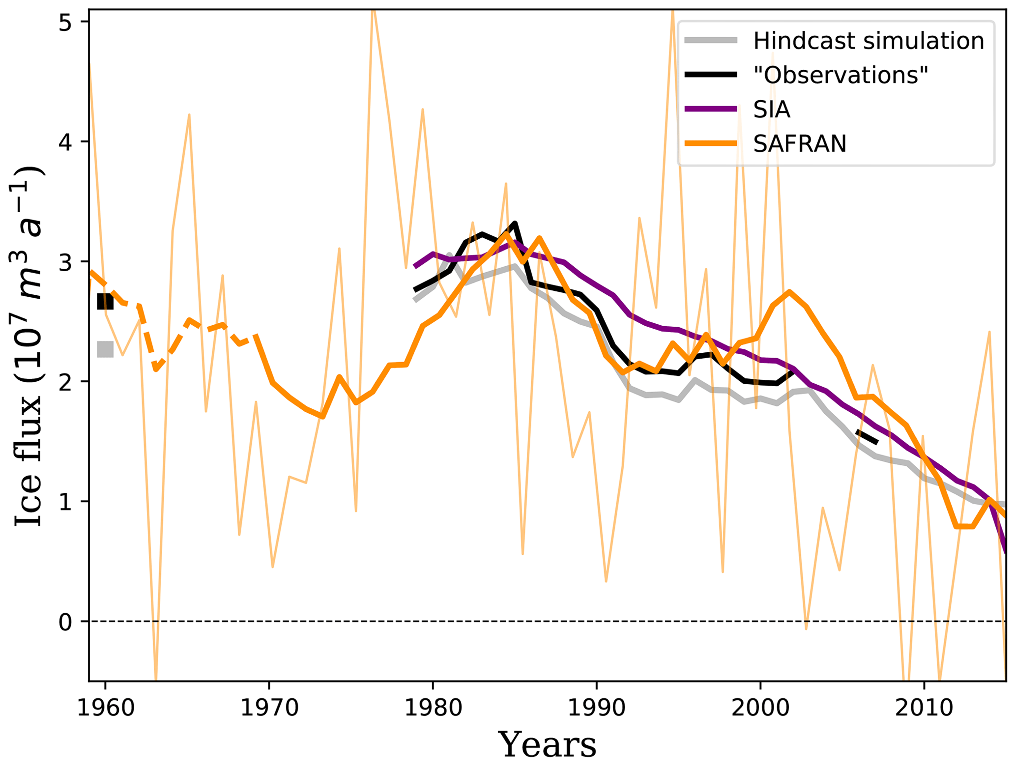
Figure 3Ice flux through the Tacul gate from 1979 to 2015 based on a previous estimate (Berthier and Vincent, 2012; in black), from the shallow ice approximation (SIA) using only observed ice thicknesses at the Tacul gate (purple), as imposed for the hindcast simulations (gray; see text) and compared to the yearly SAFRAN surface mass balance integrated upstream of the Tacul gate (thin orange) and its 11-year running mean (thick orange).
3.2.3 Flux through the Tacul gate
To account for the artificial boundaries at the Tacul and Leschaux gates, normal ice velocities over these boundaries and changes in surface elevation are imposed as Dirichlet boundary conditions for the free surface equations (Eq. 1). The treatment is different for hindcast and forecast simulations but also for Tacul and Leschaux, given that Leschaux has much less data.
In all cases, we assume that the form of the vertical profile of the horizontal velocity normal to the flux gate is given by the shallow ice approximation (SIA; Hutter, 1981). From the results of the inversion of basal friction performed over the whole domain using the 2003 observed surface velocity, we further assume a constant and uniform ratio between sliding and surface velocities of 1∕3 at both gates (). The vertical profile of the normal velocity at the gate is evaluated as
in which the deformational velocity is either imposed knowing us (hindcast simulations at Tacul),
or evaluated using the diagnostic formulation for SIA (forecast at Tacul),
In the above equations, zb is the bedrock elevation, whereas H denotes ice thickness. In Eq. (6), the surface slope ∇H is the 2003 value and is held constant with time.
The transverse profile of surface velocity is assumed to follow the 2003 SPOT5 surface velocity at the Tacul cross section (see Fig. 7b in Berthier and Vincent, 2012): it is null on the side and increases linearly from both sides of the glacier to reach a maximum central value uniform over a constant width of 400 m.
For the hindcast simulation, this maximum central value, denoted as us TAC, is given from observations, as is also the case for the ice thickness hs TAC. Knowing both the surface velocity, us=us TAC, and ice thickness, H=hs TAC, in Eq. (5) and assuming the above transverse velocity profile, the total flux through the gate can be estimated (see Fig. 2b). Despite the differences in the methods to estimate the ice flux at the gate, our inferred flux is consistent with the previous estimation of Berthier and Vincent (2012) (see Fig. 3) who assumed constant ratios of 0.8 between the width-averaged and observed centerline surface velocities and of 0.9 between depth-averaged and width-averaged surface velocities. The assumptions on transverse and vertical velocity profiles with that we use in our modeling lead, respectively, to ratios of 0.75 and 0.85, which are very close to the ones adopted by Berthier and Vincent (2012), explaining the closeness of the two approaches.
For the forecast simulations, us and H are unknown. Instead, the flux is directly evaluated from the integrated surface mass balance above the Tacul gate (see Fig. 2b) and then used to determine the value of H and the velocity distribution at the gate from Eq. (6). Ice flux through the gate is assessed by integrating, upstream of the Tacul gate, the surface mass balance given by the climate scenarios. For steady state conditions, the ice flux should be equal to the sum of the surface mass balance obtained over the whole area of the upper part. In reality, the glacier being in a highly unsteady state, this condition is not fulfilled. To estimate the relationship between ice flux at the gate and surface mass balance upstream of the gate, we use the observations made between 1979 and 2015 and the reconstructed surface mass balance using SAFRAN reanalyses (Durand et al., 2009). It is found that the observed ice flux at the Tacul gate is best estimated by averaging the surface mass balance integrated upstream of the gate over the 11 preceding years (Fig. 3). This duration corresponds approximately to the time period for the ice to flow from the lowest part of the accumulation area through the ice fall and reach the Tacul gate. The glacier has retreated for the last 3 decades and is expected to continue in the next decades. As the glacier regime will be similar in the future, it is furthermore assumed that this relationship will remain valid in the future.
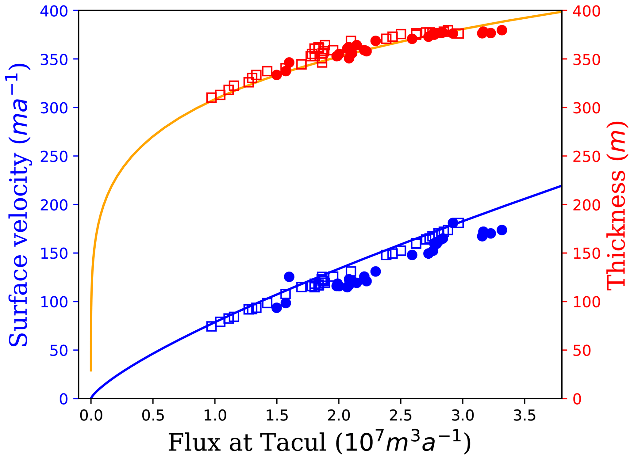
Figure 4Surface velocity (blue) and thickness (red) at the Tacul gate as a function of the flux through the gate. The curves are the analytical solutions obtained using the SIA (Eq. 6), and the squares correspond to the flux integrated by Elmer/Ice using observed surface velocity, ice thickness and a velocity distribution given by Eqs. (4) and (5). The circles are the fluxes estimated by Berthier and Vincent (2012).
The inferred relationships between ice flux, velocity and thickness at the Tacul gate are shown in Fig. 4. This figure also presents these relations for the available observations (1979–2015). Their comparison confirms the validity of the empirical relations used above. As shown in Fig. 2b, some scenarios lead to a negative integrated surface mass balance above the Tacul gate, which could result in a very small or even null flux at the gate when integrated over 11 years. To avoid a physically meaningless and overly large decrease in H (a zero flux would imply an instantaneous decrease in H to zero), the annual decrease in H at the Tacul gate is bounded by the local annual surface mass balance because the modeled thickness changes cannot be more negative than ablation. Moreover, to ensure the physical consistency of this boundary condition over the whole simulation period, surface velocity and thickness cannot be null. In applying this second condition, the minimal thickness in our simulation is always greater than 70 m. For surface velocity, a minimal condition of 10 m yr−1 is applied.
The same protocol is repeated for the Leschaux boundary condition. Unfortunately, the ice flow velocities through the Leschaux gate are only available for the year 2003 from satellite data (Berthier and Vincent, 2012). For other years, we assume that the ratio us TAC(t)∕us TAC(2003) obtained from Tacul observations is similar for the Leschaux gate. Note that in 2003, the surface velocity at the Leschaux gate was low (9 m yr−1) compared to the velocity at the Tacul gate (140 m yr−1). Its maximum ice thickness (175 m) was half of that of the Tacul gate (360 m), while their widths are similar (≈1000 m). The corresponding flux is consequently 2 orders of magnitude lower, and its effect on Mer de Glace flow is negligible during the period of interest. Therefore, for the forecast simulations, we simply assume that the thickness linearly decreases between the 2015 thickness and a null thickness in 2050. The velocity profile is then directly given by Eq. (6) without estimating a flux from the upstream accumulation.
Figures 5 and 6 show, respectively, the reconstructed surface velocity and elevation and the front position for the whole period. Results from the hindcast simulation are compared to the observations over the period 1979–2015. After this validation stage, the forecast simulations explore the range of possible evolutions corresponding to the 26 EURO-CORDEX climate scenarios.
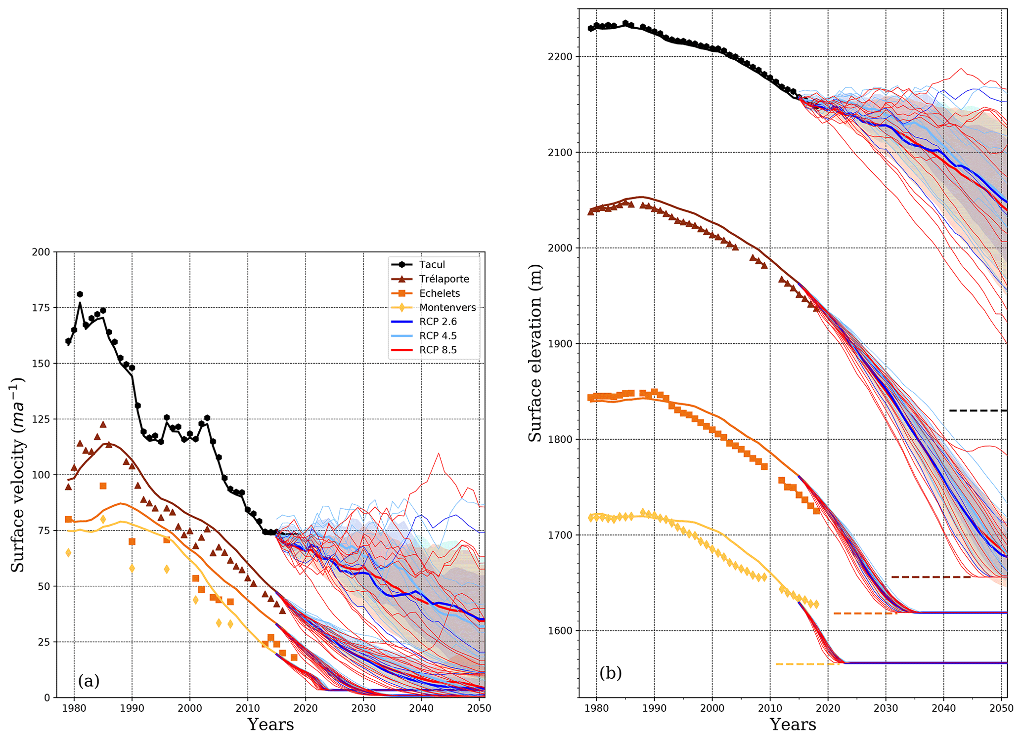
Figure 5(a) Surface velocity and (b) surface elevation for all prognostic simulations. Hindcasts at the four profiles are shown by black (Tacul), brown (Trélaporte), orange (Echelets) and yellow (Montenvers) curves, and the symbols are the corresponding observations. Forecasts are shown in dark blue (RCP 2.6), blue (RCP 4.5) and red (RCP 8.5), with the average forecasts represented by thick curves with 1σ uncertainty bands (colored area). Dashed lines indicate the bedrock elevation for the four profiles.
4.1 Hindcast simulation
For the validation of the hindcast simulation, the results of the model are compared with the centerline ice velocities (Fig. 5a) and observed surface elevation changes at the four cross sections (Fig. 5b). Note that at the highest profile (Tacul), the observations are used to impose the ice flux on this boundary of the model domain, explaining the perfect match between observations and model outputs. The validation is therefore only discussed for the three lower profiles of Trélaporte, Echelets and Montenvers.
The overall agreement of the model with the observations at the three lowest profiles was obtained without any tuning of the model parameters except the inversion of the friction coefficient using the 2003 velocity and surface elevation dataset. The model is capable of reproducing the thickening phase in the first years of the simulation period with increasing ice velocity and ice thickness, as well as the subsequent thinning phase with decreasing surface elevation and velocity. Despite this overall agreement, small differences are observed for both surface elevation and velocity.
For example, the peaks of calculated surface elevation and velocities are reached with a delay of about 3 years at Trélaporte. In the lower cross sections, Echelets and Montenvers, the surface elevation did not show a significant increase between 1979 and 1990. In general, the lower the profile is, the larger the delay will be between the onset of the decrease in the simulated compared to observed surface elevations. For the three lower cross sections, the modeled glacier is in general too thick over the last 25 years of the period compared to observations with a maximum difference of up to 25 m for Montenvers, the lowest cross section. For this cross section, this overestimation decreases in the last years before 2015, eventually becoming an underestimation. In general, the hindcast shows that the response time of thickness and velocities is too long, indicating that the modeled glacier does not respond quickly enough to the flux changes observed at the Tacul gate. The possible causes for this response delay are presented in the Discussion.
Despite these local differences in surface elevation and velocity, the general trend of snout retreat is very well reproduced by the model over the whole hindcast period (Fig. 6). The simulated front is almost stable between 1979 and 1990 and starts to retreat slowly 5 years before the observed retreat in 1995. Over the period 1995–2015, the rapid observed retreat of the ice front is well reproduced with a retreat rate of 30 m yr−1 compared to 35 m yr−1 for the observations.
Comparisons of area and volume evolution with the few available DEMs show good agreement (Fig. S3 in the Supplement). Figure 5 shows that hindcast thicknesses are slightly overestimated, and this trend is also visible in the volume evolution. The volume decrease between 1979 and 2003 (14 % of the initial volume) is underestimated by 30 %. Extent reduction (10 % of the initial area) is also underestimated by 25 %.
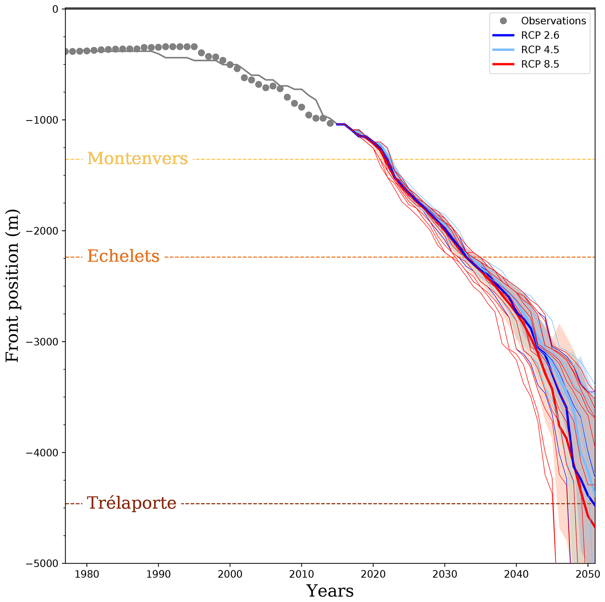
Figure 6Evolution of the front position (along a flow line defined by the front fluctuation). The hindcast is in gray, and the squares represent observations. Forecasts are shown in dark blue (RCP 2.6), blue (RCP 4.5) and red (RCP 8.5) with average forecasts represented by thick curves with 1σ uncertainty bands.
4.2 Forecast simulations
The forecast simulations were carried out using the surface mass balance calculated from the 26 climate scenarios obtained in the framework of the EURO-CORDEX program (Fig. 2). Note that all representative concentration pathways (RCPs 2.6, 4.5 or 8.5) lead to a very similar mean decrease in surface mass balance by 2050 at the Tacul gate (see Fig. 2a), with almost double the amount of ice lost by 2050 compared to 1960. Large differences between the pathway scenarios appear only after 2050 (not shown). As a direct consequence, the same trend is observed for the integrated surface mass balance above the Tacul gate (see Fig. 2b). Even if a few individual scenarios from all RCPs can lead to stable or even increasing integrated surface mass balance above the Tacul gate by 2050, the general trend for all three RCPs is a decrease in surface mass balance, and ice flux at the Tacul gate drops close to zero by 2050 in some scenarios.
All forecast simulations show significant thinning and slowing downstream of the Tacul gate (Fig. 5). At Trélaporte and Echelets gates, differences in thickness changes are within the range of ±20 and ±10 m, respectively, until 2030. Between 2020 and 2030, the thinning at Echelets gate is from 8.0 to 8.8 m yr−1 (compared to the 5.0 m yr−1 observed between 2005 and 2015). After 2030, the simulations show much larger differences induced only by the differences in surface mass balance obtained from the different climate scenarios. Note that each climate scenario influences both the ice flux through the Tacul gate and the surface mass balance over the modeled domain. At the Tacul gate, depending on the climate scenario, the surface elevation could be either stable or could decrease by 250 m by 2050. For the most pessimistic climate model (RCP 8.5), the ice thickness at the Tacul gate is only ≈80 m in 2050, whereas the most optimistic scenario leads to a thickness slightly greater than that observed in 2015 (330 m).
However, these strong differences in ice thickness and ice flux at the Tacul gate lead to much smaller absolute differences in thinning and ice flow velocity downstream of the gate; the lower the cross section is, the smaller the differences in the different scenarios will be. For instance, modeled thinning at Trélaporte only varies in a range of 2 m yr−1 between 2030 and 2040, compared to differences as large as 9 m yr−1 at the Tacul gate over the same period. Despite some scenarios indicating stable conditions at the Tacul gate, surface elevation and ice flow velocity at the three lowest profiles decrease until 2050 for all climate scenarios, indicating conditions far from steady state for the present glacier.
Our modeling results make it possible to estimate the retreat of the snout over the next decades (Fig. 6). The observed rate of retreat was 35 m yr−1 for the hindcast period 1995–2015. According to the forecast simulations, the terminus of Mer de Glace will retreat at rates varying from 60 to 85 m yr−1 between 2020 and 2030, 65 to 95 m yr−1 for the period 2030–2040, and more than 90 m yr−1 after 2040. As a consequence, the Montenvers cross section could be free of ice by 2023 and the Echelets cross section by sometime between 2031 and 2035, depending on the climate scenario (Fig. 6). For the most pessimistic scenarios, the terminus could be close to the Tacul gate by 2050.
Finally, we define a mean reference scenario constructed as the average of all 26 climate scenarios. Figure 7 presents the evolution of the ice thickness and the glacier extent for this mean reference scenario. It also illustrates the variability in glacier extent induced by the different climate scenarios up until 2050 by showing the minimum and maximum extent obtained with the 26 different scenarios for the years 2015, 2025, 2040 and 2050. This mean reference scenario is further used to study the relative contribution of ice flux at the Tacul gate and surface mass balance of the glacier tongue in the Discussion section.
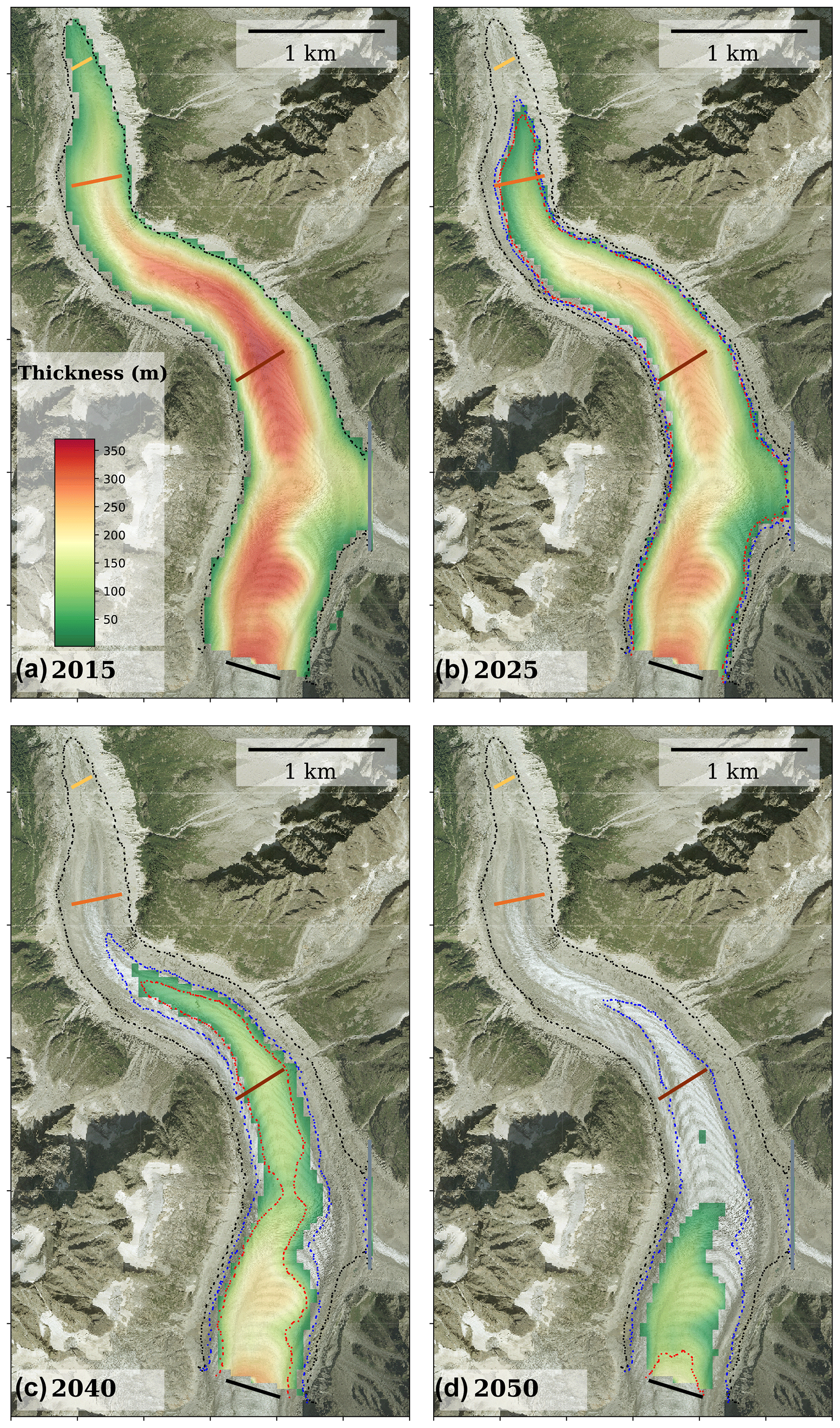
Figure 7Ice thickness and glacier extension (a) at the end of the hindcast simulation in 2015 and for the mean reference forecast simulation for the years (b) 2025, (c) 2040 and (d) 2050. The climate scenario for the mean reference forecast simulation is the average of all 26 climate scenarios. Extensions of the most optimistic and most pessimistic scenarios are plotted in dark blue and red, respectively. The initial glacier extension in 2015 is plotted in black. The background image is the orthophoto from 2008 (©RGD74).
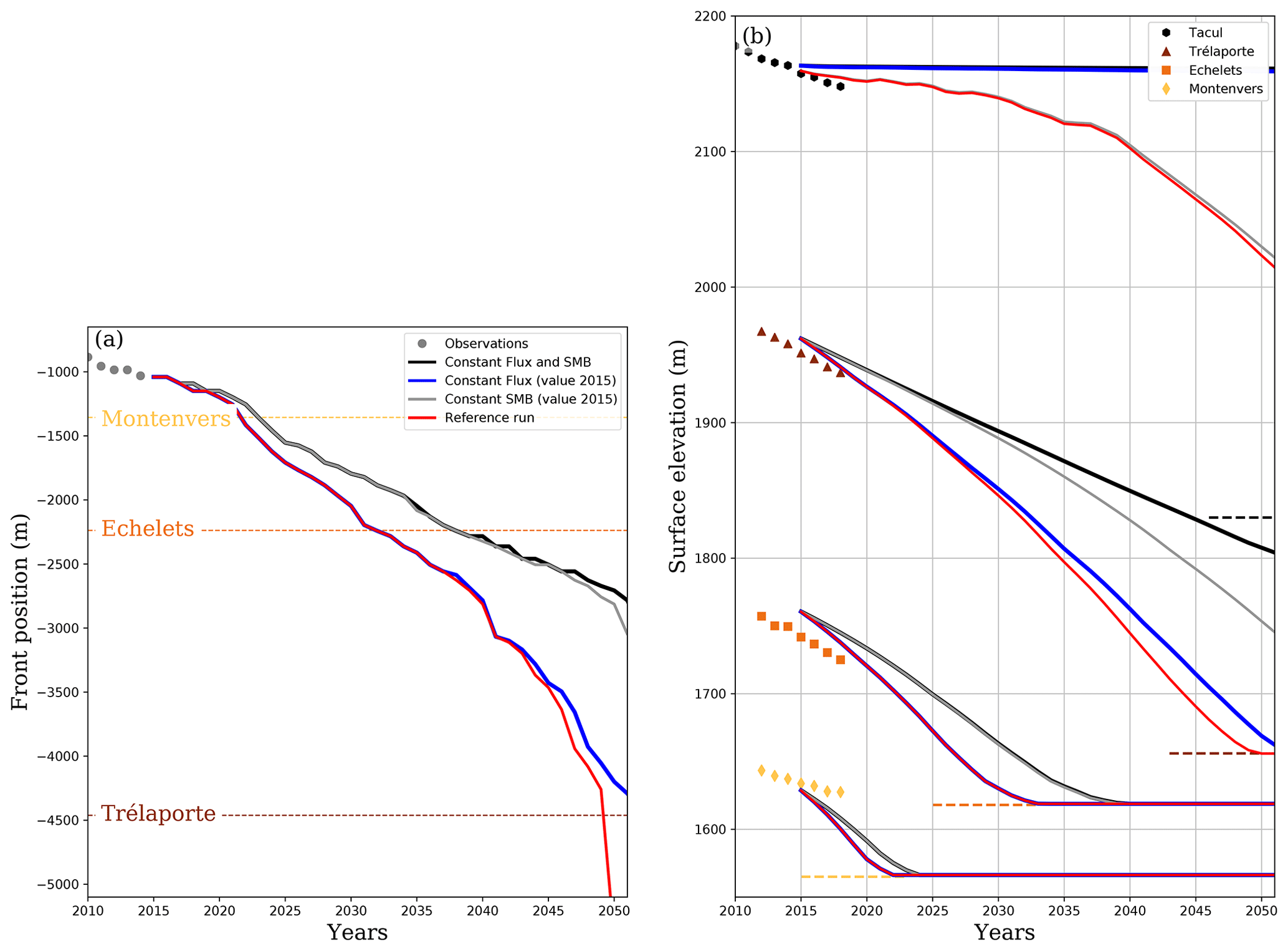
Figure 8Sensitivity experiment for the mean reference scenario assuming the mean surface mass balance of all scenarios. Evolution of (a) the glacier front and (b) the surface elevation for this mean reference scenarios (red), assuming a constant surface mass balance (gray, value from year 2015), assuming a constant flux at the Tacul gate (blue, value from year 2015) and assuming that both surface mass balance and flux at the Tacul gate are constant and equal to their 2015 values (black). Dashed lines indicate in (a) the position along the retreat line and in (b) the bedrock elevation for the gates. For the two lowest gates of Echelets and Montenvers, the red and blue curves are superimposed.
The model reproduces the evolution of the glacier over the past 4 decades relatively well. However, the observed timing and amplitude of changes are not perfectly reproduced and are increasingly inaccurate as the distance to the Tacul gate increases.
In particular, the modeled glacier underestimates the early growth and thins a few years too late. Consequently the glacier is too thick and velocity too high after 1990, resulting in a flux that is increasingly too high at the profiles of Trélaporte, Echelets and Montenvers. For the hindcast period, there is a relatively high level of confidence in the applied surface mass balance and imposed flux at the Tacul gate, both being directly derived from a continuously maintained network of stakes over the whole glacier. According to Thibert et al. (2008), we can expect uncertainties on ablation estimated from a network of stakes on the order of 0.15 m yr−1 in ice equivalent thickness, which is low relative to the mean ablation measured on the tongue of Mer de Glace (from 5 to 12 m yr−1). Other uncertainties arise from the linear extrapolation of ablation over the tongue (Eq. 3) based on measurements in an area of clean ice. Indeed, debris cover below Echelets gate has increased in recent decades and may have locally decreased ablation by up to 3 m (Fig. 3b in Berthier and Vincent, 2012). This probably explains our overestimation of the thinning rate at the Montenvers profile after 2000 (see Fig. 5b). While other studies proposed a model for the debris cover evolution and its influence (Jouvet et al., 2011), it is difficult to estimate how the debris cover will evolve above Echelets gate and influence the future retreat of Mer de Glace. Nevertheless, to test the sensitivity to the linear vertical gradient kb (Eq. 3), we performed the simulations with a lower gradient kb=0.7 . This value corresponds to the averaged gradient inferred from SAFRAN reanalysis and to the minimal gradient inferred from the climatic scenarios. For this gradient, we still assume the same surface mass balance at Tacul gate's altitude than for the gradient kb=0.9 . The lower gradient gives an ice ablation that is reduced by 1.2 m yr−1 at the front. The results are available in the Supplement (see Fig. S4). The lower gradient leads to higher discrepancies in thickness and front retreat during the hindcast. Compared to the chosen gradient, kb=0.9 , the forecast evolutions with the lower vertical gradient modestly limit the glacier thinning: Montenvers and Echelets gates are ice free after 5 years, and in 2050 the tongue is 250 to 500 m longer.
The bedrock elevation, of which measurement density has greatly improved due to a recent radar campaign over the modeled area (unpublished), is also well constrained with an estimated average uncertainty of 10 m (Vincent et al., 2009). Moreover, velocities are not systematically over or underestimated during the hindcast period, which might be an indication of a missing transient process in our simulation. The sensitivity of the results to the value of the rate factor in Glen's law has not been explored, but one should expect that a different value would only affect the ratio between ice deformation and basal sliding. Moreover, the glacier being temperate, this value should be uniform and constant and cannot therefore explain the transient discrepancy between the model and the observations. Consequently, the major process explaining these discrepancies is likely basal friction and its evolution from year to year which is not accounted for in the model. Indeed, the basal conditions are inverted from the 2003 dataset and kept constant over the whole simulation. Changes in glacier geometry and surface runoff have likely induced changes in basal conditions over the 4 decades. Inferring these changes would require contiguous surface DEMs and surface velocity maps, which are not available for dates other than 2003.
Regarding the glacier retreat, Berthier and Vincent (2012) estimated that over the period 1979–2008, two-thirds of the increase in the thinning rates observed in the lowest part of Mer de Glace was caused by reduced ice fluxes (and consequently emergence velocities) at the Tacul gate and one-third by increasing surface ablation. In other words, they estimated that the retreat of the glacier front was more influenced by changes at high elevations than local changes. With a comprehensive ice flow description for the last 4 decades and for the future, the relative contribution to glacier retreat of local vs. higher elevation changes can be quantified. As shown below, the results of our hindcast are consistent with the results of Berthier and Vincent (2012) over the period 1979–2008.
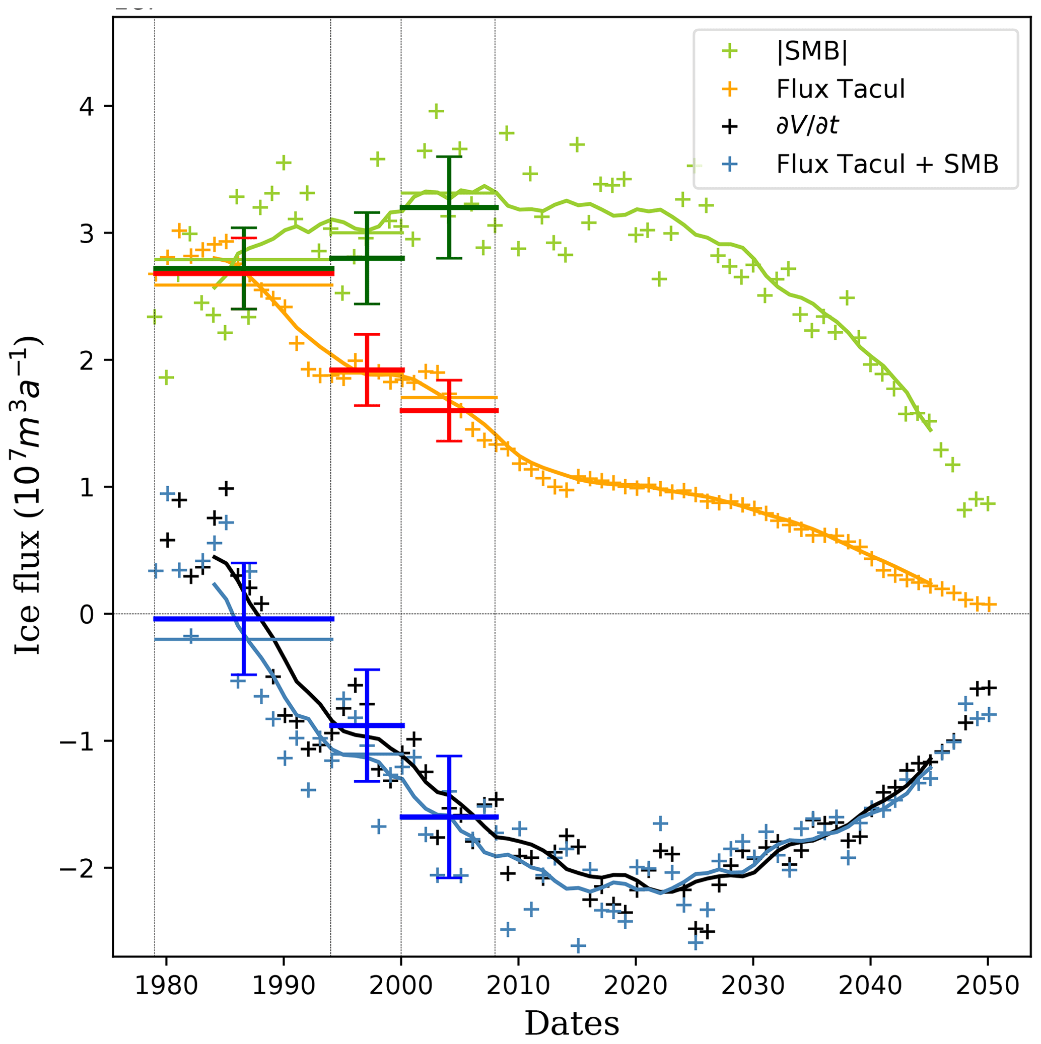
Figure 9Sensitivity experiment for the mean reference scenario assuming the mean surface mass balance of all scenarios. Evolution with time of the absolute value of the integrated surface mass balance (green, real value always negative), integrated flux at the Tacul gate (orange, always positive) and changes in volume of the glacier tongue (black) in cubic meters of ice per year. The blue curve represents the sum of the two fluxes and is almost equal to the change in volume. For each quantity, crosses represent annual values, whereas the line is a 10-year running average. The bars with error bars in dark colors are the estimates of the same quantities by Berthier and Vincent (2012) for the three periods delimited by the vertical gray lines. Horizontal lines using the same colors as the curves represent the averages of the different quantities over the same periods.
For the future, we perform a set of sensitivity experiments to test the influence of the artificial flux condition at the Tacul gate using the mean reference scenario corresponding to the mean of the 26 scenarios (e.g., mean surface mass balance and mean flux at the Tacul gate). The trends obtained for this mean reference scenario apply also to most of the other individual scenarios presented above. We perform 3 additional simulations assuming either a constant surface mass balance with the value from the year 2015, a constant flux at the Tacul gate (value from year 2015), or that both surface mass balance and flux at the Tacul gate are constant and equal to their 2015 values. Figure 8 presents the front and surface elevation evolutions for the four experiments. The experiment with only decreasing surface mass balance is close to the mean reference scenario. In comparison, simulations with a constant SMB give similar trajectories with limited thinning and front retreat. Differences due to the Tacul gate flux are mainly visible close to Trélaporte gate and are limited downstream. Contrary to the past trends, Fig. 8a clearly indicates that the future retreat of the glacier front will be influenced more by local changes (i.e., changes in surface mass balance over the lowest part of the glacier) than by changes in flux from the upstream area (i.e. flux at the Tacul gate). It is only after 2045, when the front approaches the Tacul gate, that its retreat starts to be largely influenced by changes in the upstream flux. The same trend is visible for surface elevation changes at the two lowest profiles of Echelets and Montenvers where changes in surface elevation are mostly influenced by the local surface mass balance (Fig. 8b). For the intermediate profile of Trélaporte, the influence from the flux at the Tacul gate is visible, but the local surface mass balance still dominates the observed decrease in surface elevation over the whole studied period.
Integrated surface mass balance, flux through the Tacul gate and volume changes for the mean reference simulation are plotted in Fig. 9. When surface mass balance is integrated over the glacier downstream of the Tacul gate, we can estimate the relative contributions over time of the surface mass balance and the flux at the Tacul gate to the total change in volume of the glacier tongue. As depicted in Fig. 9, surface mass balance and flux at the Tacul gate were almost equal (in absolute values) over the period 1979–1994, and the glacier tongue of Mer de Glace was very close to equilibrium, explaining an almost stationary front position over this period (Fig. 6). Nevertheless, since that period, both terms have started to decrease but not at the same rate, explaining the two-thirds contribution of flux at the Tacul gate observed by Berthier and Vincent (2012) over the period 1979–2008 and confirmed by our results. Whereas the flux at the Tacul gate has been decreasing at an almost constant rate since the mid-1980s, the rate of decrease in the tongue-integrated surface mass balance is evolving with time. As shown in Fig. 9, the tongue-integrated surface mass balance is currently reaching its minimum and is expected to increase in the future. As a consequence, the volume lost from the tongue of Mer de Glace is currently reaching its maximum and should start to decrease in the future. Indeed, even if larger melt rates are expected in the future, the tongue-integrated surface mass balance is increasing toward zero due to the decrease in the glacier tongue area. This explains why the surface mass balance over the glacier tongue is increasingly dominating changes in ice volume downstream of the Tacul gate relative to ice flux through the gate.
Because the model domain was restricted to the glacier area downstream of the Tacul gate, it was not possible to conduct simulations after 2050 for most of the scenarios. Indeed, after this date, the ice thickness at Tacul rapidly decays to zero. The choice of adopting a restricted domain for the modeling was dictated by the lack of measurements of bedrock elevation upstream. Prognostic simulations over a longer period would therefore require bedrock topography to be determined by additional mapping and/or inference using an inverse method (e.g., Fürst et al., 2018; Farinotti et al., 2019). Nevertheless, as shown by our results, the evolution of the glacier tongue is not sensitive to the boundary condition imposed at the Tacul gate. Therefore, including the upper part of the glacier in the modeled domain would not likely change the results for the studied period but would allow simulations beyond 2050.
Most studies simulating the three-dimensional geometry of a mountain glacier generally compare reconstructions with length, area or volume observations when DEMs are available (Jouvet et al., 2011; Zekollari et al., 2014). Our study allows in addition a yearly comparison of thickness and velocity changes at different locations of the glacier. The iconic status of Mer de Glace and facilities of the Électricité De France for hydropower resources and Compagnie du Mont Blanc for tourist activities justify a specific study with a state-of-the art model. It suggests that tourist facilities should be modified.
Vincent et al. (2014) used a parameterized model calibrated with past thickness changes and the surface mass balance inferred from its sensitivity to atmospheric warming to simulate the future fluctuations of Mer de Glace. They found that Mer de Glace will retreat by 1200 m by 2040 with a warming trend of 0.04 . In a new estimation using, as the present study, the EURO-CORDEX projections adjusted with the ADAMONT method, Vincent et al. (2019) found retreats of 1 to 3 km by 2050. Zekollari et al. (2019) used an SIA model to reconstruct the evolution of all glaciers located in the Alps. They used a EURO-CORDEX ensemble scenario. They found that Mer de Glace will retreat by 2 to 6 km between 2017 and 2050, which is close to our results. On a decadal timescale, retreats with the parameterized model are smaller than retreats obtained with ice flow models. It could be related to the lack of the dynamics in the parameterized model. Another explanation is that parameterized models take into account the local thickness and surface mass balance changes given that they are based on in situ observations.
The future evolution of the glacier can also be related to its response time which has been a subject of interest of several studies. The response times of glaciers are affected by several predictors such as the glacier size, the glacier SMB and glacier slope, which is the main driver. Recently, Zekollari et al. (2020) used large-scale glacier modeling to investigate the response time in the European Alps. For Mer de Glace, the relationship proposed by the authors between average surface slope, elevation range and the response time gives a response time of 60 years, which is typical of the range of European Alps glaciers (50±28 years). Our sensitivity experiments confirm this result. Indeed, the future simulation performed with stationary flux at Tacul and surface mass balance after 2015 shows that Mer de Glace will reach a steady state after 70 years and a front retreat of 4.1 km.
Finally, Jouvet and Huss (2019) lead forecast simulations for the Great Aletsch glacier, the largest glacier in the European Alps, with a full Stokes model and the EURO-CORDEX ensemble. Their results are close to those of Zekollari et al. (2019). They predict a glacier retreat of around 5 km between 2017 and 2050, which is similar to the Mer de Glace forecasts.
In this study, the Elmer/Ice ice flow model was applied to simulate the past and future evolution of the lower part of Mer de Glace. Given that the bedrock elevation remains unknown in the upper part of the glacier, we specified the ice fluxes at the Tacul and Leschaux gates which are the upper limits of the tongue. These ice fluxes were obtained from monitored cross-section surface area and ice flow velocities for hindcast. For forecasts, they were assessed from the simulated surface mass balance in the accumulation zone.
The simulation of the glacier tongue for the period 1979 to 2015 was driven by (i) surface mass balance measurements and (ii) the ice flux at the Tacul and Leschaux gates, which were obtained directly from the observed surface area and ice flow velocities. Ice flow modeling results were compared to detailed and continuous observations of surface elevation, surface velocity and snout fluctuations over 4 decades during which the glacier experienced both a period of increase and a long period of decay. To our knowledge, a comparison to data in this detail is unprecedented. We found that our modeling using Elmer/Ice is able to reproduce the general behavior of the glacier. For example, the early growth of the glacier occurring between 1979 and 1990 is correctly reconstructed. However, the elevation increase is underestimated in the lower part of the tongue. After 1990, the modeling results are in agreement with observations. We suspect that the small differences between the model and the observations arise from the constant basal friction parameter imposed over the hindcast period. Additional uncertainties in the surface mass balance of the tongue are likely related to the sparse debris cover.
Using 26 climate scenarios, the model was run forward to simulate the evolution of the glacier tongue until 2050. There were major differences in the ice fluxes calculated at the Tacul gate from all these scenarios; however, changes in velocity and elevation at the lowest part of the glacier, as well as the retreat of the glacier front, were shown to be relatively independent of this upstream flux. Indeed, our sensitivity study indicates that the future changes at the lowest cross sections of the tongue are mainly influenced by the local surface mass balance, which depends on the distance from the upper gate where the ice flux is prescribed. This also explains why the upper cross section of Trélaporte is more sensitive to the upstream flux condition at Tacul. Because of the decreasing surface area, the rate of volume loss from the glacier downstream of the Tacul gate is currently reaching a maximum and will continue decreasing in the future. The glacier snout could retreat by 2 to 6 km over the next 3 decades and be close to the Tacul gate by 2050.
Forecast simulations over a longer period would require extension of the model domain upstream of the Tacul gate, which is hindered by the unknown bedrock topography. Radar measurements in the upper part of Mer de Glace and/or inverse modeling are therefore required to estimate the bedrock topography in this area before realistic forecast simulations of Mer de Glace can be extended beyond 2050.
Elmer/Ice code is publicly available through GitHub (https://github.com/ElmerCSC/elmerfem, last access: 3 November 2020, Gagliardini et al., 2013).
The supplement related to this article is available online at: https://doi.org/10.5194/tc-14-3979-2020-supplement.
VP, CV, CB and OG designed the experiments. VP, CB and FG-C performed the numerical modeling. OL, DS, and CV performed the geophysical and geodetic measurements. VP led the writing of the paper with contribution from all coauthors.
The authors declare that they have no conflict of interest.
We thank Samuel Morin and Deborah Verfaillie (Centre d'Etude de la Neige, Météo France/CNRS) who produced the climate scenarios used in this study (ADAMONT simulations, https://opensource.umr-cnrm.fr/projects/adamont, last access: 3 November 2020). Remote field measurements were obtained thanks to the support of the TOSCA program of the French Space Agency (CNES). Glaciological data were obtained from the GLACIOCLIM database, https://glacioclim.osug.fr/ (last access: 3 November 2020). This study was supported by Électricité de France and Compagnie du Mont Blanc. We thank all collaborators past and present for their thorough measurements of mass balance, thickness and velocity changes, as well as bedrock topography, for Mer de Glace over all these decades. We thank the editor Andreas Vieli and the three anonymous reviewers for their judicious comments and suggestions that greatly improved the quality of the initial paper.
This paper was edited by Andreas Vieli and reviewed by three anonymous referees.
Berthier, E. and Vincent, C.: Relative contribution of surface mass-balance and ice-flux changes to the accelerated thinning of Mer de Glace, French Alps, over 1979-2008, J. Glaciol., 58, 501–512, https://doi.org/10.3189/2012JoG11J083, 2012. a, b, c, d, e, f, g, h, i, j, k, l, m
Berthier, E., Arnaud, Y., Baratoux, D., Vincent, C., and Rémy, F.: Recent rapid thinning of the ”Mer de Glace” glacier derived from satellite optical images, Geophys. Res. Lett., 31, L17401, https://doi.org/10.1029/2004GL020706, 2004. a, b
Berthier, E., Vadon, H., Baratoux, D., Arnaud, Y., Vincent, C., Feigl, K. L., Rémy, F., and Legresy, B.: Surface motion of mountain glaciers derived from satellite optical imagery, Remote Sens. Environ., 95, 14–28, https://doi.org/10.1016/j.rse.2004.11.005, 2005. a
Berthier, E., Vincent, C., Magnússon, E., Gunnlaugsson, Á. Þ., Pitte, P., Le Meur, E., Masiokas, M., Ruiz, L., Pálsson, F., Belart, J. M. C., and Wagnon, P.: Glacier topography and elevation changes derived from Pléiades sub-meter stereo images, The Cryosphere, 8, 2275–2291, https://doi.org/10.5194/tc-8-2275-2014, 2014. a
Braithwaite, R. J.: Positive degree-day factors for ablation on the Greenland ice sheet studied by energy-balance modelling, J. Glaciol., 41, 153–160, https://doi.org/10.3189/S0022143000017846, 1995. a
Brunner, M. I., Gurung, A. B., Zappa, M., Zekollari, H., Farinotti, D., and Stähli, M.: Present and future water scarcity in Switzerland: Potential for alleviation through reservoirs and lakes, Sci. Total Environ., 666, 1033–1047, https://doi.org/10.1016/j.scitotenv.2019.02.169, 2019. a
Clarke, G. K. C., Jarosch, A. H., Anslow, F. S., Radić, V., and Menounos, B.: Projected deglaciation of western Canada in the twenty-first century, Nat. Geosci., 8, 372–377, https://doi.org/10.1038/ngeo2407, 2015. a
Durand, Y., Laternser, M., Giraud, G., Etchevers, P., Lesaffre, B., and Mérindol, L.: Reanalysis of 44 yr of climate in the French Alps (1958–2002): Methodology, model validation, climatology, and trends for air temperature and precipitation, J. Appl. Meteorol. Clim., 48, 429–449, https://doi.org/10.1175/2008JAMC1808.1, 2009. a, b, c
Farinotti, D., Brinkerhoff, D. J., Clarke, G. K. C., Fürst, J. J., Frey, H., Gantayat, P., Gillet-Chaulet, F., Girard, C., Huss, M., Leclercq, P. W., Linsbauer, A., Machguth, H., Martin, C., Maussion, F., Morlighem, M., Mosbeux, C., Pandit, A., Portmann, A., Rabatel, A., Ramsankaran, R., Reerink, T. J., Sanchez, O., Stentoft, P. A., Singh Kumari, S., van Pelt, W. J. J., Anderson, B., Benham, T., Binder, D., Dowdeswell, J. A., Fischer, A., Helfricht, K., Kutuzov, S., Lavrentiev, I., McNabb, R., Gudmundsson, G. H., Li, H., and Andreassen, L. M.: How accurate are estimates of glacier ice thickness? Results from ITMIX, the Ice Thickness Models Intercomparison eXperiment, The Cryosphere, 11, 949–970, https://doi.org/10.5194/tc-11-949-2017, 2017. a
Farinotti, D., Huss, M., Fürst, J. J., Landmann, J., Machguth, H., Maussion, F., and Pandit, A.: A consensus estimate for the ice thickness distribution of all glaciers on Earth, Nat. Geosci., 12, 168–173, https://doi.org/10.1038/s41561-019-0300-3, 2019. a
Fürst, J. J., Navarro, F., Gillet-Chaulet, F., Huss, M., Moholdt, G., Fettweis, X., Lang, C., Seehaus, T., Ai, S., Benham, T. J., Benn D. I., Björnsson H., Dowdeswell J. A., Mariusz Grabiec, G., Kohler, J., Lavrentiev, I., Lindbäck, K., Melvold, K., Pettersson, R., Rippin, D., Saintenoy, A., Pablo Sánchez-Gámez, P., Schuler, T. V., Sevestre, H., Vasilenko, E., and Braun, M. H.: The Ice-Free Topography of Svalbard, Geophys. Res. Lett., 45, 11–760, https://doi.org/10.1029/2018GL079734, 2018. a
Gagliardini, O., Gillet-Chaulet, F., Durand, G., Vincent, C., and Duval, P.: Estimating the risk of glacier cavity collapse during artificial drainage: The case of Tête Rousse Glacier, Geophys. Res. Lett., 38, L10505, https://doi.org/10.1029/2011GL047536, 2011. a
Gagliardini, O., Zwinger, T., Gillet-Chaulet, F., Durand, G., Favier, L., de Fleurian, B., Greve, R., Malinen, M., Martín, C., Råback, P., Ruokolainen, J., Sacchettini, M., Schäfer, M., Seddik, H., and Thies, J.: Capabilities and performance of Elmer/Ice, a new-generation ice sheet model, Geosci. Model Dev., 6, 1299–1318, https://doi.org/10.5194/gmd-6-1299-2013, 2013. a, b, c
Gerbaux, M., Genthon, C., Etchevers, P., Vincent, C., and Dedieu, J.: Surface mass balance of glaciers in the French Alps: distributed modeling and sensitivity to climate change, J. Glaciol., 51, 561–572, https://doi.org/10.3189/172756505781829133, 2005. a
Gilbert, A., Sinisalo, A., Gurung, T. R., Fujita, K., Maharjan, S. B., Sherpa, T. C., and Fukuda, T.: The influence of water percolation through crevasses on the thermal regime of a Himalayan mountain glacier, The Cryosphere, 14, 1273–1288, https://doi.org/10.5194/tc-14-1273-2020, 2020. a, b, c
Gillet-Chaulet, F., Gagliardini, O., Seddik, H., Nodet, M., Durand, G., Ritz, C., Zwinger, T., Greve, R., and Vaughan, D. G.: Greenland ice sheet contribution to sea-level rise from a new-generation ice-sheet model, The Cryosphere, 6, 1561–1576, https://doi.org/10.5194/tc-6-1561-2012, 2012. a
Glen, J. W.: The creep of polycrystalline ice, P. R. Soc. A, 228, 519–538, 1955. a
Gluck, S.: Détermination du lit rocheux sous la Mer de Glace par séismique-réflexion, CR Acad. Sci., 264, 2272–2275, 1967. a
Greuell, W.: Hintereisferner, Austria: mass-balance reconstruction and numerical modelling of the historical length variations, J. Glaciol., 38, 233–244, https://doi.org/10.3189/S0022143000003646, 1992. a
Haeberli, W. and Hölzle, M.: Application of inventory data for estimating characteristics of and regional climate-change effects on mountain glaciers: a pilot study with the European Alps, Ann. Glaciol., 21, 206–212, https://doi.org/10.1017/S0260305500015834, 1995. a
Hock, R.: Temperature index melt modelling in mountain areas, J. Hydrol., 282, 104–115, https://doi.org/10.1016/S0022-1694(03)00257-9, 2003. a
Hock, R., Bliss, A., Marzeion, B., Giesen, R. H., Hirabayashi, Y., Huss, M., Radić, V., and Slangen, A. B. A.: GlacierMIP – A model intercomparison of global-scale glacier mass-balance models and projections, J. Glaciol., 65, 453–467, https://doi.org/10.1017/jog.2019.22, 2019. a
Huss, M.: Extrapolating glacier mass balance to the mountain-range scale: the European Alps 1900–2100, The Cryosphere, 6, 713–727, https://doi.org/10.5194/tc-6-713-2012, 2012. a
Huss, M. and Hock, R.: Global-scale hydrological response to future glacier mass loss, Nat. Clim. Change, 8, 135–140, https://doi.org/10.1038/s41558-017-0049-x, 2018. a, b
Huss, M., Farinotti, D., Bauder, A., and Funk, M.: Modelling runoff from highly glacierized alpine drainage basins in a changing climate, Hydrol. Process., 22, 3888–3902, https://doi.org/10.1002/hyp.7055, 2008. a
Hutter, K.: The effect of longitudinal strain on the shearstress of an ice sheet: in defence of using stretched coordinates, J. Glaciol., 27, 39–56, https://doi.org/10.3189/S0022143000011217, 1981. a
Huybrechts, P., de Nooze, P., and Decleir, H.: Numerical modelling of glacier d'Argentière and its historic front variations, in: Glacier Fluctuations and Climatic Change, edited by: Oerlemans, J., 373–389, https://doi.org/10.1007/978-94-015-7823-3_24, 1989. a
IPCC: High Mountain Areas, in: IPCC Special Report on the Ocean and Cryosphere in a Changing Climate, Cambridge University Press, available at: https://www.ipcc.ch/srocc (last access: 3 November 2020), 2019. a, b
Jacob, D., Petersen, J., Eggert, B., Alias, A., Christensen, O. B., Bouwer, L. M., Braun, A., Colette, A., Déqué, M., Georgievski, G., Georgopoulou, E., Gobiet, A., Menut, L., Nikulin, G., Haensler, A., Hempelmann, N., Jones, C., Keuler, K., Kovats, S., Kröner, N., Kotlarski, S., Kriegsmann, A., Martin, E., van Meijgaard, E., Moseley, C., Pfeifer, S., Preuschmann, S., Radermacher, C., Radtke, K., Rechid, D., Rounsevell, M., Samuelsson, P., Somot, S., Soussana, J.-F., Teichmann, C., Valentini, R., Vautard, R., Weber, B., and Yiou, P.: EURO-CORDEX: new high-resolution climate change projections for European impact research, Reg. Environ. Change, 14, 563–578, https://doi.org/10.1007/s10113-013-0499-2, 2014. a
Jouvet, G. and Huss, M.: Future retreat of Great Aletsch Glacier, J. Glaciol., 65, 869–872, https://doi.org/10.1017/jog.2019.52, 2019. a, b
Jouvet, G., Huss, M., Funk, M., and Blatter, H.: Modelling the retreat of Grosser Aletschgletscher, Switzerland, in a changing climate, J. Glaciol., 57, 1033–1045, https://doi.org/10.3189/002214311798843359, 2011. a, b
Kääb, A., Leinss, S., Gilbert, A., Bühler, Y., Gascoin, S., Evans, S. G., Bartelt, P., Berthier, E., Brun, F., Chao, W.-A., Farinotti, D., Gimbert, F. Guo, W., Huggel, C., Kargel, J. S., Leonard, G. J., Tian, L., Treichler, D., and Yao, T.: Massive collapse of two glaciers in western Tibet in 2016 after surge-like instability, Nat. Geosci., 11, 114–120, https://doi.org/10.1038/s41561-017-0039-7, 2018. a
Le Meur, E. and Vincent, C.: A two-dimensional shallow ice-flow model of Glacier de Saint-Sorlin, France, J. Glaciol., 49, 527–538, https://doi.org/10.3189/172756503781830421, 2003. a
Letréguilly, A. and Reynaud, L.: Past and Forecast Fluctuations of Glacier Blanc (French Alps), Ann. Glaciol., 13, 159–163, https://doi.org/10.3189/S0260305500007813, 1989. a
Lliboutry, L., Vallon, M., and Vivet, R.: Étude de trois glaciers des Alpes Françaises, in: Union Géodésique et Géophysique Internationale, Association Internationale d'Hydrologie Scientifique, Commission des Neiges et des Glaces, Colloque d'Obergurgl, 10–18 September 1962, 145–59, 1962. a
Marzeion, B., Jarosch, A. H., and Hofer, M.: Past and future sea-level change from the surface mass balance of glaciers, The Cryosphere, 6, 1295–1322, https://doi.org/10.5194/tc-6-1295-2012, 2012. a
Marzeion, B., Hock, R., Anderson, B., Bliss, A., Champollion, N., Fujita, K., Huss, M., Immerzeel, W., Kraaijenbrink, P., Malles, J.-H., Maussion, F., Radìc, V., Rounce, D. R., Sakai, A., Shannon, S., van de Wal, R., and Zekollari, H.: Partitioning the Uncertainty of Ensemble Projections of Global Glacier Mass Change, Earths Future, 8, e2019EF001470, https://doi.org/10.1029/2019EF001470, 2020. a, b
Maussion, F., Butenko, A., Champollion, N., Dusch, M., Eis, J., Fourteau, K., Gregor, P., Jarosch, A. H., Landmann, J., Oesterle, F., Recinos, B., Rothenpieler, T., Vlug, A., Wild, C. T., and Marzeion, B.: The Open Global Glacier Model (OGGM) v1.1, Geosci. Model Dev., 12, 909–931, https://doi.org/10.5194/gmd-12-909-2019, 2019. a
Millan, R., Mouginot, J., Rabatel, A., Jeong, S., Cusicanqui, D., Derkacheva, A., and Chekki, M.: Mapping Surface Flow Velocity of Glaciers at Regional Scale Using a Multiple Sensors Approach, Remote Sens.-Basel, 65, 2498, https://doi.org/10.3390/rs11212498, 2019. a
Oerlemans, J.: Glaciers and climate change: a meteorologist's view., A. A. Balkema Publishers, 2001. a
Paterson, W. S. B.: The Physics of Glaciers, 3rd edn., Elsevier Science Ltd, 1994. a
Rabatel, A., Dedieu, J.-P., and Vincent, C.: Using remote-sensing data to determine equilibrium-line altitude and mass-balance time series: validation on three French glaciers, 1994–2002, J. Glaciol., 51, 539–546, https://doi.org/10.3189/172756505781829106, 2005. a
Radić, V., Bliss, A., Beedlow, A. C., Hock, R., Miles, E., and Cogley, J. G.: Regional and global projections of twenty-first century glacier mass changes in response to climate scenarios from global climate models, Clim. Dynam., 42, 37–58, https://doi.org/10.1007/s00382-013-1719-7, 2014. a
Réveillet, M., Rabatel, A., F., G.-C., and Soruco, A.: Simulations of changes to Glaciar Zongo, Bolivia (16∘ S), over the 21st century using a 3-D full-Stokes model and CMIP5 climate projections, Ann. Glaciol., 56, 89–97, https://doi.org/10.3189/2015AoG70A113, 2015. a, b
Réveillet, M., Vincent, C., and Six, D. Rabatel, A.: Which empirical model is best suited to simulate glacier mass balances?, J. Glaciol., 63, 39–54, https://doi.org/10.1017/jog.2016.110, 2017. a, b, c, d
Six, D. and Vincent, C.: Sensitivity of mass balance and equilibrium-line altitude to climate change in the French Alps, J. Glaciol., 60, 867–878, https://doi.org/10.3189/2014JoG14J014, 2014. a
Solomon, S., Qin, D., Manning, M., Averyt, K., and Marquis, M.: Climate change 2007 – the physical science basis: Working group I contribution to the fourth assessment report of the IPCC, vol. 4, Cambridge University Press, 2007. a
Stewart, E. J., Wilson, J., Espiner, S., Purdie, H., Lemieux, C., and Dawson, J.: Implications of climate change for glacier tourism, Tourism Geogr., 18, 377–398, https://doi.org/10.1080/14616688.2016.1198416, 2016. a
Stroeven, A., van de Wal, R., and Oerlemans, J.: Historic front variations of the Rhone Glacier: simulation with an ice flow model, in: Glacier Fluctuations and Climate Change, edited by: Oerlemans, J., Springer, Dordrecht, 391–405, 1989. a
Süustrunk, A. E.: Sondage du glacier par la méthode sismique, Houille Blanche, No. spécial A, 309–318, https://doi.org/10.1051/lhb/1951010, 1951. a
Thibert, E., Blanc, R., Vincent, C., and Eckert, N.: Glaciological and volumetric mass-balance measurements: error analysis over 51 years for Glacier de Sarennes, French Alps, J. Glaciol., 54, 522–532, https://doi.org/10.3189/002214308785837093, 2008. a
Vallon, M.: Épaisseur du glacier du Tacul (massif du Mont- Blanc), CR Acad. Sci., 252, 1815—1817, 1961. a
Vallon, M.: Contribution à l'étude de la Mer de Glace., Ph.D. thesis, Université de Grenoble, 1967. a
Vallot, J.: Tome I à VI, in: Annales de l'Obsevatoire météoprologique, physique et glaciaire du Mont Blanc (altitude 4,358 métres), G Steinheil, Paris, 1905. a
Verfaillie, D., Déqué, M., Morin, S., and Lafaysse, M.: The method ADAMONT v1.0 for statistical adjustment of climate projections applicable to energy balance land surface models, Geosci. Model Dev., 10, 4257–4283, https://doi.org/10.5194/gmd-10-4257-2017, 2017. a
Verfaillie, D., Lafaysse, M., Déqué, M., Eckert, N., Lejeune, Y., and Morin, S.: Multi-component ensembles of future meteorological and natural snow conditions for 1500 m altitude in the Chartreuse mountain range, Northern French Alps, The Cryosphere, 12, 1249–1271, https://doi.org/10.5194/tc-12-1249-2018, 2018. a
Vincent, C.: Influence of climate change over the 20th Century on four French glacier mass balances, J. Geophys. Res., 107, 4375, https://doi.org/10.1029/2001JD000832, 2002. a
Vincent, C., Soruco, A., Six, D., and Le Meur, E.: Glacier thickening and decay analysis from 50 years of glaciological observations performed on Glacier d'Argentière, Mont Blanc area, France, Ann. Glaciol., 50, 73–79, https://doi.org/10.3189/172756409787769500, 2009. a
Vincent, C., Harter, M., Gilbert, A., Berthier, E., and Six, D.: Future fluctuations of Mer de Glace, French Alps, assessed using a parameterized model calibrated with past thickness changes, Ann. Glaciol., 55, 15–24, https://doi.org/10.3189/2014AoG66A050, 2014. a, b, c, d
Vincent, C., Peyaud, V., Laarman, O., Six, D., Gilbert, A., Gillet-Chaulet, F., Berthier, E., Morin, S., Verfaillie, D., Rabatel, A., Jourdain, B., and Bolibar, J.: Déclin des deux plus grands glaciers des Alpes françaises au cours du XXI siècle: Argentière et Mer de Glace, La Météorologie, 106, 49–58, https://doi.org/10.4267/2042/70369, 2019. a
Vionnet, V., Six, D., Auger, L., Dumont, M., Lafaysse, M., Quéno, L., Réveillet, M., Dombrowski-Etchevers, I., Thibert, E., and Vincent, C.: Sub-kilometer Precipitation Datasets for Snowpack and Glacier Modeling in Alpine Terrain, Front. Earth Sci., 7, 182, https://doi.org/10.3389/feart.2019.00182, 2019. a
Welling, J. T., Árnason, Þ., and Ólafsdottír, R.: Glacier tourism: A scoping review, Tourism Geogr., 17, 635–662, https://doi.org/10.1080/14616688.2015.1084529, 2015. a
Zekollari, H., Fürst, J. J., and Huybrects, P.: Modelling the evolution of Vadret da Morteratsch, Switzerland, since the Little Ice Age and into the future, J. Glaciol., 60, 1155–1168, https://doi.org/10.3189/2014JoG14J053, 2014. a
Zekollari, H., Huss, M., and Farinotti, D.: Modelling the future evolution of glaciers in the European Alps under the EURO-CORDEX RCM ensemble, The Cryosphere, 13, 1125–1146, https://doi.org/10.5194/tc-13-1125-2019, 2019. a, b, c
Zekollari, H., Huss, M., and Farinotti, D.: On the Imbalance and Response Time of Glaciers in the European Alps, Geophys. Res. Let., 47, e2019GL085578, https://doi.org/10.1029/2019GL085578, 2020. a
Zemp, M., Haeberli, W., Hoelzle, M., and Paul, F.: Alpine glaciers to disappear within decades?, Geophys. Res. Lett., 33, L13504, https://doi.org/10.1029/2006GL026319, 2006. a
Zemp, M., Frey, H., Gärtner-Roer, I., and Nussbaumer, S. U.”: Historically unprecedented global glacier decline in the early 21st century, J. Glaciol., 61, 745–762, https://doi.org/10.3189/2015JoG15J017, 2015. a
Zemp, M., Huss, M., Thibert, E., Eckert, N., McNabb, R., Huber, J., Barandun, M., Machguth, H., Nussbaumer, S. U., Gärtner-Roer, I., Thomson, L., Paul, F., Maussion, F., Kutuzov, S., and Cogley, J. G.: Global glacier mass changes and their contributions to sea-level rise from 1961 to 2016, Nature, 568, 382–386, https://doi.org/10.1038/s41586-019-1071-0, 2019. a