the Creative Commons Attribution 4.0 License.
the Creative Commons Attribution 4.0 License.
 | 11 Nov 2020
GrSMBMIP: intercomparison of the modelled 1980–2012 surface mass balance over the Greenland Ice Sheet
Xavier Fettweis
Stefan Hofer
Uta Krebs-Kanzow
Charles Amory
Teruo Aoki
Constantijn J. Berends
Andreas Born
Jason E. Box
Alison Delhasse
Koji Fujita
Paul Gierz
Heiko Goelzer
Edward Hanna
Akihiro Hashimoto
Philippe Huybrechts
Marie-Luise Kapsch
Michalea D. King
Christoph Kittel
Charlotte Lang
Peter L. Langen
Jan T. M. Lenaerts
Glen E. Liston
Gerrit Lohmann
Sebastian H. Mernild
Uwe Mikolajewicz
Kameswarrao Modali
Ruth H. Mottram
Masashi Niwano
Brice Noël
Jonathan C. Ryan
Amy Smith
Jan Streffing
Marco Tedesco
Willem Jan van de Berg
Michiel van den Broeke
Roderik S. W. van de Wal
Leo van Kampenhout
David Wilton
Bert Wouters
Florian Ziemen
Tobias Zolles
Observations and models agree that the Greenland Ice Sheet (GrIS) surface mass balance (SMB) has decreased since the end of the 1990s due to an increase in meltwater runoff and that this trend will accelerate in the future. However, large uncertainties remain, partly due to different approaches for modelling the GrIS SMB, which have to weigh physical complexity or low computing time, different spatial and temporal resolutions, different forcing fields, and different ice sheet topographies and extents, which collectively make an inter-comparison difficult. Our GrIS SMB model intercomparison project (GrSMBMIP) aims to refine these uncertainties by intercomparing 13 models of four types which were forced with the same ERA-Interim reanalysis forcing fields, except for two global models. We interpolate all modelled SMB fields onto a common ice sheet mask at 1 km horizontal resolution for the period 1980–2012 and score the outputs against (1) SMB estimates from a combination of gravimetric remote sensing data from GRACE and measured ice discharge; (2) ice cores, snow pits and in situ SMB observations; and (3) remotely sensed bare ice extent from MODerate-resolution Imaging Spectroradiometer (MODIS). Spatially, the largest spread among models can be found around the margins of the ice sheet, highlighting model deficiencies in an accurate representation of the GrIS ablation zone extent and processes related to surface melt and runoff. Overall, polar regional climate models (RCMs) perform the best compared to observations, in particular for simulating precipitation patterns. However, other simpler and faster models have biases of the same order as RCMs compared with observations and therefore remain useful tools for long-term simulations or coupling with ice sheet models. Finally, it is interesting to note that the ensemble mean of the 13 models produces the best estimate of the present-day SMB relative to observations, suggesting that biases are not systematic among models and that this ensemble estimate can be used as a reference for current climate when carrying out future model developments. However, a higher density of in situ SMB observations is required, especially in the south-east accumulation zone, where the model spread can reach 2 m w.e. yr−1 due to large discrepancies in modelled snowfall accumulation.
- Article
(15749 KB) - Full-text XML
-
Supplement
(268 KB) - BibTeX
- EndNote


Mass loss from the Greenland Ice Sheet (GrIS) has been accelerating since the 1990s (Enderlin et al., 2014; Mouginot et al., 2019; Hanna et al., 2020; IMBIE2, 2020). Over the period 1992–2018, roughly 50 % of the total mass loss can be ascribed to reduced GrIS surface mass balance (SMB) (IMBIE2, 2020):
which refers to the difference between the total precipitation (rain and snow, P), meltwater runoff (RU), sublimation/evaporation (SU), snow erosion by the wind (ER) and glacier storage (GS). Since drifting snow erosion contributes ∼ 1 Gt yr−1 (i.e. < 0.3 %) to the SMB, ER is neglected in most models, although it can be important locally (Lenaerts et al., 2012). Moreover, the glacial water storage (supraglacial lakes, melt ponds, rivers) is neglected in this intercomparison, as it is not simulated by any model considered here. However, the mass changes coming from GS could be relevant when the SMB is integrated over the whole ice sheet but have never been quantified until now.
Since the end of the 1990s, the models suggest that the surface melt has almost doubled, reaching record melt volume in the summers of 2012 and 2019, while the snowfall accumulation has remained approximately constant (Noël et al., 2019; Lenaerts et al., 2019; Tedesco and Fettweis, 2020). This recent GrIS SMB decrease – largely driven by the increase in meltwater runoff (Van den Broeke et al., 2016; Fettweis et al., 2017; Lenaerts et al., 2019; IPCC, 2019) – has been caused by Arctic amplification, a state change in the North Atlantic Oscillation and increased Greenland Blocking events in summer (Fettweis et al., 2013b; Delhasse et al., 2018; Hanna et al., 2018; Hahn et al., 2020), which raise the average temperatures (Screen and Simmonds, 2010), reduce the cloudiness (Hofer et al., 2017) and enhance the melt–albedo feedback (Box et al., 2012; Ryan et al., 2019; Noël et al., 2019). While models agree well with satellite-based reconstructions, large uncertainties and model discrepancies remain in the current SMB evolution (IMBIE2, 2020). Additionally, SMB-related processes are one of the main uncertainties in future projections of the GrIS contribution to sea level rise as the ice sheet retreats in a warmer climate (Goelzer et al., 2013; van den Broeke et al., 2017; Hofer et al., 2019).
Therefore, there is a pressing need to improve and refine model estimates of recent SMB changes, for which we have in situ measurements and satellite data sets, in order to subsequently reduce the large model spread in future GrIS SMB projections. With the aim of reducing uncertainties in current modelled SMB estimates, we compare four types of SMB model, using 13 models in total to (i) create an accurate multi-models SMB reconstruction over current climate and an associated uncertainty based on the ensemble of these models and (ii) discuss the added values and drawbacks of each of them. Prior to this study, only a few attempts were made to compare the available models in terms of their ability to simulate the contemporary GrIS SMB (e.g. Vernon et al., 2013). These previous studies (i) evaluated SMB within a subset of regional climate models (RCMs) (Rae et al., 2012), (ii) compared positive degree day (PDD) models with energy balance snowpack models (van de Wal, 1996; Bougamont et al., 2007) or (iii) assessed the representation of specific physical sub-processes (Reijmer et al., 2012). Since these models implement different physical and statistical processes, are run on different grids, use different forcing data, and/or cover various temporal ranges, previous model comparison studies suffer from limited inter-comparability.
In this study, we compare the SMB outputs of 13 state-of-the-art (physical and statistical) climate models (1) over a common time period (1980–2012), (2) using a common, 1 km spatial grid and (3) over a common ice-sheet mask using the contemporary GrIS extent. Moreover, 11 out of the 13 participating models are forced with ERA-Interim reanalysis (Dee et al., 2011), although each model prescribes the reanalysis forcing in a different manner.
Four kinds of models participate in our intercomparison:
-
Positive degree day (PDD) models using near-surface summer temperature to estimate melt and precipitation from forcing. The melt parameterizations of these models are relatively simple and due to the underlying assumptions they depend notably on the near-surface climate of their forcing (for precipitation in particular). However, the computational costs are very low and therefore they can be run at very high spatial resolutions and over long timescales.
-
Energy balance models (EBMs) compute the surface energy balance to estimate melt by deriving surface energy fluxes and precipitation from forcing. Although the representation of surface melt is physically more robust than PDDs and they are able to simulate feedbacks including the melt–albedo feedback, they are also very dependent on the near-surface climate from the forcing data. However, similar to PDDs, EBMs are also computationally efficient. Therefore, both PDDs and EBMs are particularly useful to downscale large-scale fields with the aim of forcing ice sheet models over long periods.
-
Regional climate models (RCMs) coupled with energy-balance-based snow models compute energy fluxes, precipitation and the near-surface climate at a high resolution over the ice sheet. RCMs are forced at their lateral boundaries by global fields, mostly temperature, humidity and general circulation. A priori, they provide the best approach to represent the melt and precipitation patterns, as well as to simulate the surface–atmosphere interactions at a high resolution. It is for this reason that the present SMB estimations of the Greenland Ice Sheet are mainly based on RCMs forced by reanalyses (IMBIE2, 2020). However, RCMs are computationally very expensive, typically limiting their simulations to 100 years. Finally, their results remain dependent on the biases in the forcing free-atmosphere fields above and around Greenland (Fettweis et al., 2013a).
-
General circulation models (GCMs) are global models that, unlike RCMs, have no spatial boundary conditions. Instead, they require a small set of time-dependent primary inputs, such as aerosol emissions, greenhouse concentrations and land use. Coupled with energy-balance-based snow models, GCMs are capable of simulating GrIS SMB, which is particularly useful to perform future projections. However, to maintain reasonable computational time, their spatial resolution remains low, limiting their ability to explicitly simulate the snow–atmosphere interactions in the narrow ablation zone or the topography-induced precipitation. Coupled with an ice sheet model, GCMs are the only tools that explicitly represent changes in general circulation in ocean or atmosphere, resulting from thinning of the ice sheet and other feedback processes.
For both PDDs and EBMs, the models are forced by the ERA-Interim near-surface climate extrapolated to the model's spatial resolution. In RCMs, the reanalysis data set is prescribed at the ocean surface and at the lateral boundaries of their integration domain. Two types of GCM configurations are used in this study, (i) one using an active ocean component, i.e. a truly free-running set-up, and (ii) an atmosphere-only configuration, where reconstructed historical sea surface temperatures and sea ice cover are used as the boundary conditions over the ocean, possibly resulting in a modelled climate more closely resembling the real world (AMIP experiment; see Gates et al., 1998).
Sections 2 and 3 describe the 13 models used in the intercomparison (2 PDDs, 4 EBMs, 5 RCMs and 2 GCMs) and the observational data sets used for the evaluation of these models. The models are inter-compared in Sect. 4 by highlighting the main discrepancies between models and evaluated in Sect. 5 with in situ observations and satellite data. In Sect. 6, the discrepancies between models identified in Sect. 4 are linked to biases highlighted in Sect. 5 to propose the best estimates of the mean SMB and SMB changes over the current climate (1980–2012). Finally, conclusions are drawn in Sect. 7. Note that this intercomparison exercise aims to reduce uncertainty and identify regions with low measurement density and large model discrepancies in order to provide some insight into regional uncertainty; it is not the purpose here to formally rank model performance.
Table 1List of the 13 models used in this study listing the type (energy balance model (EBM), regional climate model (RCM), general circulation model (GCM), positive degree day (PDD) model), the forcing (the ERA-Interim or JRA-55 reanalysis), the native resolution, the method eventually used afterwards to downscale the surface mass balance (SMB) at 1 km (when it is different than the one use to interpolate all the outputs to 1 km; see Sect. 2.2) and the country where the main development takes place.
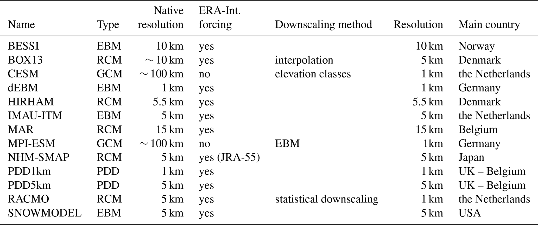
A brief description of each of the 13 models used in this study is provided in the following section and summarized in Table 1.
2.1 Description of the participating models
2.1.1 BESSI (EBM – 10 km)
BESSI is a surface energy and mass balance model designed for simulating long timescales (Born et al., 2019; Zolles and Born, 2019). It is forced with ERA-Interim reanalysis fields of temperature, humidity, longwave and shortwave radiation, and precipitation (Dee et al., 2011). The temperature is the only variable that is downscaled to the actual model topography (ETOPO1, Amante and Eakins, 2009) using a lapse rate of 0.0065 K m−1. Contrary to previously published model versions, here we use incoming longwave radiation as a forcing field rather than a temperature-based parameterization. Energy fluxes are calculated with a time step of one day on a 10×10 km2 grid.
The model uses an albedo scheme based on a linear relationship between temperature and a time decay rate (Aoki et al., 2003). This decay is enhanced in the presence of liquid water in the surface layer. The latent and sensible turbulent heat fluxes are calculated based on the residual method (Rolstad and Oerlemans, 2005; Braithwaite, 2009) with constant wind speed over the entire ice sheet. Refreezing and percolation is instantaneous in every time step, with a maximum water holding capacity of 10 % of the free pore volume (Greuell, 1992). Finally, the model parameters were optimized to fit the GRACE mass balance data over the 2002–2018 period (Born et al., 2019).
2.1.2 BOX13 (calibrated RCM – 5 km)
The basis of the BOX13 surface mass balance reconstruction are linear regression parameters that describe relationships between spatially discontinuous in situ records from meteorological stations (i.e. monthly temperature after Vinther et al., 2006; Cappelen et al., 2001, 2006; Cappelen, 2011) or firn/ice cores and spatially continuous outputs from the version 2.1 of the regional climate model RACMO (Ettema et al., 2010), described in Sect. 2.1.12. Explanatory (independent variable) data (air temperature and firn/ice core data) span 1840 to 2012. A 43-year overlap period 1960–2012 with RACMO2.1 is used to determine regression parameters on a grid cell basis. A fundamental assumption is that the calibration factors, regression slope and offset for the calibration period 1960–2012 are stationary over time.
The RACMO2.1 data are resampled and reprojected from a 0.1∘ (∼ 10 km) grid to a 5 km grid. See “part I” of Box et al. (2013) for a description of the method, which includes a formal approach to estimate uncertainty. The following refinements are, however, made from the SMB reconstruction of Box et al. (2013) and Box (2013). The estimation of values is made for a domain that includes not only ice but land and sea. The physically based meltwater retention scheme of Pfeffer et al. (1991) replaced the simpler approach used by Box (2013). Multiple station records contribute to the near-surface air temperature for each given year, month and grid cell in the domain, while in Box (2013), only data from the single highest correlating station yielded the reconstructed value. These revised surface mass balance data end with year 2012, while Box (2013) data end in 2010. Finally, the annual accumulation rates from ice cores are dispersed into a monthly temporal resolution by weighting the monthly (based on the 1960–2012 RACMO2.1 data) fraction of the annual total for each grid cell in the domain. The accumulation reconstruction has been evaluated by Lewis et al. (2017, 2019).
2.1.3 CESM2 (GCM – 1 km)
In this study, the CESM version 2.0 (CESM2) is used in a configuration with a fixed ocean state. In particular, the protocol for the Atmospheric Model Intercomparison Project (AMIP, Gates et al., 1999) is used, with prescribed sea surface temperatures and sea ice cover from Hurrell et al. (2008) for the period 1979–2014. Global land cover usage is also prescribed. The atmospheric and land components are the Community Atmosphere Model version 6 (CAM6) and the Community Land Model version 5 (CLM5), respectively, both operating at a nominal resolution of 1∘. No ice dynamics are considered; i.e. the geometry of the GrIS is static over time. Initial conditions for CAM6 and CLM5 snow packs are taken from a fully coupled CESM2 simulation. Sub-grid topographic variability is partially accounted for by the use of multiple elevation classes (ECs) in CLM5, with up to 10 ECs per grid cell. Atmospheric forcing is downscaled to each EC, with lapse rates used for temperature and downwelling longwave radiation and phase recomputation for precipitation (for details, see Van Kampenhout et al., 2020). Output indexed by EC is used for downscaling CESM2 SMB to the 1 km ISMIP6 grid (Nowicki et al., 2016) using linear interpolation in the vertical and bilinear interpolation in the horizontal direction. A detailed evaluation of present-day GrIS climate and SMB in CESM2 has been published in Van Kampenhout et al. (2020).
2.1.4 dEBM (EBM – 1 km)
The diurnal Energy Balance Model (dEBM, Krebs-Kanzow et al., 2020) is a surface mass balance scheme that incorporates both radiative and turbulent heat fluxes and captures diurnal variability in the melt–freeze cycles (Krebs-Kanzow et al., 2018) and monthly variations in cloud cover. For forcing, dEBM version employed here only requires monthly means of shortwave radiation at the surface, near-surface air temperature and precipitation. Monthly mean duration and intensity of the diurnal melting and refreezing periods are derived from the monthly mean surface radiation and from the diurnal cycle of the top of atmosphere (TOA) shortwave radiation. The latter is implicitly represented as a function of latitude and month based on prescribed parameters of the Earth's orbit around the Sun. Monthly mean atmospheric transmissivity and cloud cover are estimated from the ratio between monthly mean shortwave radiation at the surface and at the TOA (from forcing fields and from orbital parameters, respectively). The scheme has a monthly time step and distinguishes albedo of bare ice and wet, dry and new snow on the basis of precipitation, surface energy balance and the previous month's snow type and snow height. Additionally, the scheme includes a residual heat flux R which is thought to represent those energy fluxes which are not included in the scheme, such as the heat flux to the subsurface or latent heat fluxes at the surface. Here, R has been treated as a tuning parameter and has been optimized to W m−2 with respect to the surface mass balance measurements from Machguth et al. (2016) over the ERA-Interim period (1979–2016). To force the model, monthly mean ERA-Interim precipitation, surface insolation and near-surface air temperatures have been interpolated to the 1 km ISMIP6 grid and temperature fields have been additionally downscaled by applying a lapse rate correction of K m−1.
2.1.5 HIRHAM (RCM – 5.5 km)
The HIRHAM regional climate model has been developed to include a full surface energy and mass balance model using an original code developed from physical schemes used in the ECHAM5 global model and dynamical schemes from the HIRLAM numerical weather prediction model. It has 31 vertical levels and is forced on 6-hourly intervals on the lateral boundaries. The RCM has a simple five-layer snowpack model to a depth of 10 m over glacier surfaces, incorporating the same parameterizations used in an offline version that has 32 layers. The offline version assimilates MODIS MOD10A albedo data to get a closer fit between modelled and observed albedos. Langen et al. (2017) describe the snowpack model in detail and show that the inclusion of MODIS data significantly improves the modelled SMB.
2.1.6 IMAU-ITM (EBM – 5 km)
IMAU-ITM is an insolation- and temperature-based SMB model. This simplified EBM is used in the ANICE ice-sheet model for paleoclimate simulations (de Boer et al., 2014; Berends et al., 2018). Monthly precipitation from the ERA-Interim reanalysis is downscaled to actual model topography (in this case, the BedMachine v3 data set; Morlighem et al., 2017) using the wind-orography-based parameterization by Roe and Lindzen (2001) and Roe (2002). The resulting downscaled precipitation is partitioned into rain and snow based on the temperature parameterization by Ohmura (1999). The depth of the accumulated snow layer is tracked, with a maximum value of 10 m; any additional firn is assumed to be compressed into ice. The surface albedo is calculated as a weighted average of the albedos of fresh snow and bare ice, based on the thickness of the snow layer and the amount of melt that occurred during the previous year. Melt is determined using the insolation-temperature parameterization by Bintanja et al. (2002), which uses prescribed values for insolation at the top of the atmosphere, and which was developed especially for paleoglaciological applications. Refreezing is calculated following the approach by Huybrechts and de Wolde (1999) and Janssens and Huybrechts (2000), based on the available liquid water (the sum of rain and melt) and the refreezing potential, integrated over the entire year to account for the retention of summer melt which is refrozen in winter. For this study, the parameters in the refreezing and snowmelt parameterizations were calibrated to obtain the closest match (i.e. highest value of linear correlation coefficient divided by RMSE) to the RACMO2.3 values over the 1979–2017 period on the 1 km grid.
2.1.7 MAR (RCM – 15 km)
The version 3.9.6 from MAR is used here with a resolution of 15 km. MAR was forced at its lateral boundaries by ERA-Interim at a 6-hourly time step. The boundary forcing files include information about the temperature, u and v wind components, specific humidity, and sea level pressure as well as the sea surface temperature and sea ice cover over ocean. It is the same model configuration which is used in the Ice Sheet Model Intercomparison Project for CMIP6 (ISMIP6) for future projections over the GrIS (Nowicki et al., 2016). With respect to the version 3.5.2 of MAR used in Fettweis et al. (2017) and Hofer et al. (2017), the main improvements are as follows: (1) an increase in the cloud lifetime with the aim of correcting the biases of solar and infrared radiation highlighted in Fettweis et al. (2017), (2) adjustments in the bare ice albedo representation for a better comparison with in situ measurements, (3) a larger independence of model results to the time step used and (4) a better dynamical stability with an increased spatial filtering for a computing time divided by a factor of 2 compared to version 3.5.2. Additionally, we also dealt with minor bug corrections and small updates for enhanced computing efficiency and comparison with in situ automatic weather data (Delhasse et al., 2020).
2.1.8 MPI-ESM (GCM – 1 km)
The historical simulation underlying the SMB calculations by the Max Planck Institute (MPI) is simulated with a higher-resolution version of the latest version of the MPI Earth System Model (MPI-ESM1.2-HR). In this version the atmospheric model ECHAM6.3, with a spectral resolution of T127 (∼ 100 km), is coupled to the ocean model MPIOM version 1.6.2, with a nominal 0.4∘ resolution and a tripolar grid. A thorough description of this model set-up can be found in Müller et al. (2018).
An EBM approach is used to calculate the SMB from one ensemble member of the historical MPI-ESM1.2-HR simulations (Mauritsen et al., 2019) and downscale it from ∼ 100 km to the 1 km ISMIP6 topography. The offline EBM scheme is similar to the one presented in Vizcaíno et al. (2010); despite technical changes and the introduction of elevation classes it was mainly the albedo parameterization that was updated. The EBM calculates melt and accumulation rates from hourly atmospheric fields of the historical MPI-ESM1.2-HR simulation on its native grid. The atmospheric fields are bi-linearly interpolated onto 24 fixed elevation classes, ranging from 0 to 8000 m. To account for height differences between each elevation class and the surface elevation of the atmospheric model a height correction is applied to near-surface air temperature, humidity, dew point temperature, precipitation, downward longwave radiation and near-surface density fields. The downward shortwave radiation is kept constant, as it is largely affected by atmospheric properties that are independent of elevation differences (e.g. ozone concentration, aerosol thickness) (Yang et al., 2006). To obtain melt rates, the EBM computes the energy balance at the atmosphere–snow interface as the sum over the radiative and turbulent as well as rain-induced and conductive heat fluxes. The albedo parameterization used here is based on the parameterization by Oerlemans and Knap (1998) and considers snow ageing, snow depth and the influence of cloud coverage. The obtained 3-D fields of surface melt, accumulation and SMB are then vertically and horizontally interpolated onto the 1 km ISMIP6 topography used as reference topography in this study.
2.1.9 NHM-SMAP (RCM – 5 km)
The latest version of the polar RCM NHM-SMAP, with a horizontal resolution of 5 km, developed by Niwano et al. (2018), was used in this study. The same version was recently utilized to assess cloud radiative effects on the Greenland Ice Sheet surface melt (Niwano et al., 2019). The atmospheric part of NHM-SMAP is the Japan Meteorological Agency Non-Hydrostatic atmospheric Model (JMA-NHM) developed by Saito et al. (2006), which employs flux form equations in spherical curvilinear orthogonal coordinates as the governing basic equations. We pay close attention to the cloud microphysics processes; therefore, the version of JMA-NHM utilized for NHM-SMAP (Hashimoto et al., 2017) employs a double-moment bulk cloud microphysics scheme to predict both the mixing ratio and the concentration of solid hydrometeors (cloud ice, snow and graupel), and a single-moment scheme to predict the mixing ratio of liquid hydrometeors (cloud water and rain). For the simulation of snow and ice physical conditions, the multilayered physical snowpack model SMAP is utilized (Niwano et al., 2012, 2014). The SMAP model calculates snow albedo using the detailed physically based snow albedo model developed by Aoki et al. (2011) considering the effects of snow grain size evolution explicitly. Although the model can also consider the effects of light-absorbing impurities on snow albedo, we assumed the pure snow condition here. On the other hand, bare ice albedo is calculated by using a simple parameterization as a function of density. To estimate realistic runoff from the ice sheet, a detailed vertical water movement scheme based on the Richards equation (Yamaguchi et al., 2012) is used. To force NHM-SMAP (dynamical downscaling), we used not the ERA-Interim reanalysis but the JRA-55 reanalysis (Kobayashi et al., 2015) due to the lack of enough computational resources. However, it should be noted that the quality of the arctic atmospheric physical conditions from both reanalysis data sets during the study period were almost the same level as reported by Simmons and Poli (2015) and Fettweis et al. (2017), who showed no significant difference between MAR forced by ERA-Interim and JRA-55.
2.1.10 PDD5km (PDD – 5 km)
European Centre for Medium-Range Weather Forecasts (ECMWF) ERA-Interim (Dee et al., 2011) 2 m surface air temperature, precipitation and surface latent heat flux reanalysis data were downscaled from their native 0.75∘ resolution to 5×5 km2 using bilinear interpolation, a high-resolution digital elevation model (DEM) (Ekholm, 1996) and empirically derived ice-sheet surface lapse rates to correct surface air temperature, as described in full in Hanna et al. (2005, 2011). Downscaled surface air temperature was validated using independent in situ observational automatic weather station data from the Greenland Climate Network (Steffen and Box, 2001), showing very good agreement between downscaled/modelled and observed temperatures. Net solid precipitation (snowfall minus evaporation and sublimation) was spatially calibrated against the Bales et al. (2009) kriged map of snow accumulation based on ice-core and coastal precipitation gauges. Evaporation and sublimation were calculated from surface latent heat flux. The resulting downscaled Greenland climate gridded data were used to drive a runoff/retention model (Janssens and Huybrechts, 2000) that produced surface melt, runoff, evaporation and SMB at a monthly time resolution, while net precipitation was taken from the ERA-I data set and downscaled, calibrated and adjusted as above. Ice-sheet averaged annual SMB since 1958 was shown to correlate strongly between this method and RACMO2.1 but significant differences in absolute values between the respective methods were considered to be mainly due to poorly constrained modelled accumulation (Hanna et al., 2011).
2.1.11 PDD1km (PDD – 1 km)
The modelling method is essentially the same as described in Sect. 2.1.10. However, here a higher-resolution DEM (Bamber et al., 2013) was used to downscale ERA-Interim reanalysis data to 1×1 km2 resolution, producing monthly output for 1979–2012 (Wilton et al., 2017). In addition, variable “sigma” values – standard deviation of 6-hourly temperatures, computed for each month – were incorporated into the PDD method, based on earlier work by Jowett et al. (2015). The resulting high-resolution PDD model output was evaluated using PROMICE observations (Machguth et al., 2016), showing generally robust correlations (Wilton et al., 2017) which were broadly comparable, though not quite as good, as the polar RCMs. Finally, this method is particularly useful for long centennial/pre-satellite timescales for which relatively few reliable meteorological fields are available (Wilton et al., 2017).
2.1.12 RACMO2.3 (RCM – 1 km)
The polar (p) version of the Regional Atmospheric Climate Model (RACMO2.3p2) is run at 5.5 km horizontal resolution for the period 1958–2018 (Noël et al., 2019). The model incorporates the dynamical core of the High-Resolution Limited Area Model (HIRLAM; Undèn et al., 2002) and the physics from the European Centre for Medium-range Weather Forecasts-Integrated Forecast System (ECMWF-IFS cycle CY33r1; ECMWF-IFS, 2008). RACMO2.3p2 includes a multi-layer snow module that simulates melt, water percolation and retention in snow, refreezing and runoff (Ettema et al., 2010). The model also accounts for dry snow densification (Ligtenberg et al., 2018) and drifting snow erosion and sublimation (Lenaerts et al., 2012). Snow albedo is calculated based on snow grain size, cloud optical thickness, solar zenith angle and impurity concentration in snow (Van Angelen et al., 2012). Bare ice albedo is prescribed from the 500 m MODIS 16 d albedo product (MCD43A3), as the lowest 5 % of the surface albedo records for the period 2000–2015, minimized at 0.30 for dark bare ice and maximized at 0.55 for bright ice under perennial firn. Glacier outlines and surface topography are prescribed from a down-sampled version of the 90 m Greenland Ice Mapping Project (GIMP) DEM (Howat et al., 2014). RACMO2.3p2 is forced at its lateral boundaries by ERA-40 (1958–1978) (Uppala et al., 2005) and ERA-Interim (1979–2018) (Dee et al., 2011) reanalyses on a 6-hourly basis within a relaxation zone that is 24 grid cells wide. The forcing consists of temperature, specific humidity, pressure, wind speed and direction being prescribed at each of the 40 vertical atmosphere model levels. Upper atmosphere relaxation (nudging) is also implemented in RACMO2.3p2 (Van de Berg and Medley, 2016). The model has 40 active snow layers that are initialized in September 1957 using temperature and density profiles derived from the offline IMAU Firn Densification Model (IMAU-FDM) (Ligtenberg et al., 2018). Detailed description of the model and recent updates are discussed in Noël et al. (2018, 2019).
The 5.5 km product is further statistically downscaled onto a 1 km grid to resolve the steep SMB gradients over narrow glaciers and confined ablation zones at the rugged ice sheet margins. Statistical downscaling corrects runoff for biases in elevation and bare ice albedo using a down-sampled version of the GIMP DEM (topography and ice mask) and a MODIS albedo product at 1 km resolution. This allows the high runoff rates observed at the GrIS margins to be accurately represented, significantly improving the agreement with SMB measurements. A detailed description of the statistical downscaling procedure is given in Noël et al. (2016).
2.1.13 SnowModel (EBM – 5 km)
SnowModel was forced with ERA-Interim (ERA-I) reanalysis products on a 0.75∘ longitude × 0.75∘ latitude grid from the European Centre for Medium-Range Weather Forecasts (ECMWF; Dee et al., 2011), where the 6 h (precipitation at 12 h) temporal resolution ERA-I data were downscaled to 3-hourly values and a 5 km grid. SnowModel (Liston and Elder, 2006a) contains six sub-models, where five of the models were used here to quantify spatio-temporal variations in atmospheric forcing, GrIS surface snow properties (including refreezing and retention), sublimation, evaporation, runoff and SMB. The sub-model MicroMet (Liston and Elder, 2006b; Mernild et al., 2006) downscaled and distributed the spatio-temporal atmospheric fields using the Barnes objective interpolation scheme, where the interpolated fields were also adjusted using known meteorological algorithms, e.g. temperature–elevation, wind–topography, humidity–cloudiness and radiation–cloud–topography relationships (Liston and Elder, 2006b). Enbal (Liston, 1995; Liston et al., 1999) simulated a full surface energy balance considering the influence of cloud cover, sun angle, topographic slope and aspect on incoming solar radiation, and moisture exchanges, e.g. multilayer heat- and mass-transfer processes within the snow (Liston and Mernild, 2012). SnowTran-3D (Liston and Sturm, 1998, 2002; Liston et al., 2007) accounted for the snow (re)distribution by wind. SnowPack-ML (Liston and Mernild, 2012) simulated multilayer snow depths, temperatures and water-equivalent evolutions. HydroFlow (Liston and Mernild, 2012) simulated watershed divides, routing network, flow residence time, runoff routing (configurations based on the hypothetical gridded topography and ocean-mask data sets) and discharge hydrographs for each grid cell including from catchment outlets. These sub-models have been tested against independent observations with success in Greenland, the Arctic, high mountain regions and on the Antarctic Ice Sheet with acceptable results (e.g. Liston and Hiemstra, 2011; Mernild and Liston, 2012; Mernild et al., 2015; Beamer et al., 2016).
2.2 Interpolation on a common grid
One of the key issues raised by the first SMB model intercomparison performed by Vernon et al. (2013) was the high dependency of modelled integrated SMB values to the ice sheet mask used. To mitigate this problem, we interpolate all model outputs to the same 1 km grid used in the Ice Sheet Model Intercomparison Project for CMIP6 (ISMIP6). This resolution is chosen because the highest resolution model outputs (e.g. RACMO2.3p2) are available at 1 km and choosing a coarser resolution could compromise their quality. A common grid also allows a comparison on two common ice sheet masks: the contiguous Greenland Ice Sheet, which is common to all the models and the Greenland Ice Sheet plus peripheral ice caps and mountain glaciers, common to all the models except the two PDD models. Unless otherwise indicated, the SMB components have been interpolated to 1 km using a simple linear interpolation metric of the four nearest inverse-distance-weighted model grid cells. Moreover, as done in Le clec’h et al. (2019), the interpolated 1 km SMB and runoff fields have been corrected for elevation differences between the model native topography and the GIMP 250 m topography (upscaled to 1 km here), using time- and space-varying SMB–elevation gradients, similar to Franco et al. (2012) and Noël et al. (2016). No correction was applied to precipitation after interpolation to 1 km. Finally, the ensemble mean is based on the average of the 13 modelled monthly outputs interpolated onto the common 1 km grid.
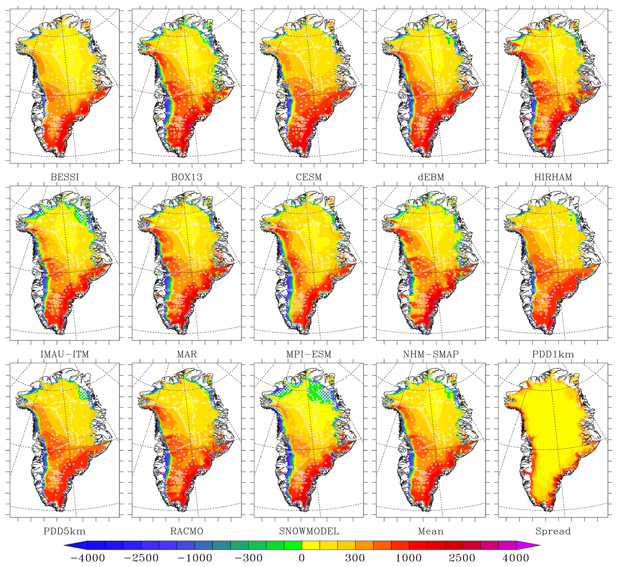
Figure 1Mean SMB (in mm w.e. yr−1) over 1980-2012 simulated by the 13 models as well as the ensemble model mean and the spread around this mean. The SMB measurements (ice cores + PROMICE) used to evaluate the models are represented as white circles. The areas listed in Table 4 where SMB disagree with the satellite-derived bare ice area are shown in a hatched area. Finally, it is important to note that for better visibility, the scale is not linear as it uses a step of 100 for absolute values lower than 500 mm w.e. yr−1 and a step of 500 above.
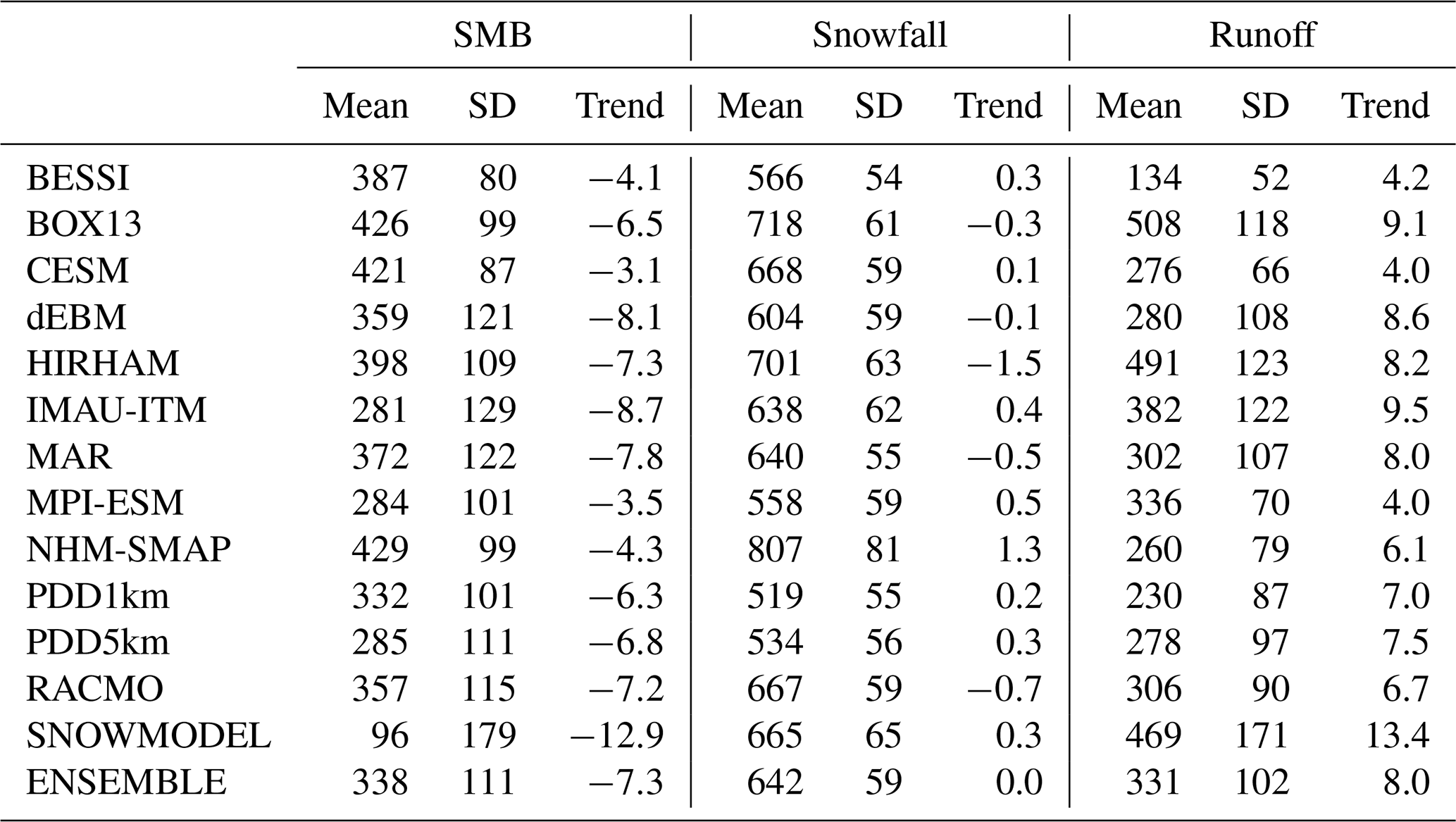
Table 2Mean, interannual variability (standard deviation of the annual means) and linear trend of the main ice sheet SMB, snowfall and runoff in (Gt yr−1) over 1980–2012 simulated by the 13 models.
3.1 Ice core and SMB measurements
Similar to Fettweis et al. (2017), we compare modelled SMB with in situ observations from the following:
-
Ice core measurements in the accumulation zone (Bales et al., 2001, 2009; Ohmura et al., 1999). The model outputs are averaged over the overlapping measurements period. We use the annual mean over 1980–2012 when the measurements period is not specified or not included into the period 1980–2012, to increase the number of available ice core measurements for model evaluation, as the snowfall accumulation has remained approximately constant over recent decades (Fettweis et al., 2017). The modelled SMB values are compared to ice cores by interpolating the four nearest inverse-distance-weighted grid cells to the common 1 km ISMIP6 grid.
-
Airborne radar transects in the accumulation zone from Karlsson et al. (2016, 2020). For all of these measurements, the annual mean over 1980–2012 is used as comparison, and as for the ice cores, outputs are interpolated using the four nearest inverse-distance-weighted grid cells to the common 1 km ISMIP6 grid.
-
The SMB database (Machguth et al., 2016) compiled under the auspice of PROMICE and available through the PROMICE web portal (http://www.promice.dk, last access: 27 October 2020). This data set mainly covers the ablation zone of the GrIS and includes measurements over some peripheral ice caps (as shown in Fig. 1). Measurements not included in the 1980–2012 period and records shorter than 3 months or located outside the common 1 km ice mask are discarded from the comparison. In a similar fashion as in Wilton et al. (2017), monthly model outputs are weighted by the length of the observed month, e.g. if the record starts in the middle of a month. Daily outputs, available for some models, are not used here, and as for the ice cores, outputs are interpolated using the four nearest inverse-distance-weighted grid cells onto the ISMIP6 ice mask.
-
The unpublished database of snow pits (Jason Box, personal communication, 2019) incorporating observations of winter accumulation over previously exposed bare ice or firn. Snow pits were monitored at the end of the following winter accumulation period (usually in May). As only the date when the snow pits were dug is known (May), we assume, for the comparison with the models, that each record started on 1 September. However, for some years and locations, the winter accumulation may have started slightly later in October or November, after some late-season melt events. That is why we have accumulated modelled SMB values from September to May when the monthly modelled SMB is positive.
3.2 GRACE estimation
The GRACE-based product, coupled with an estimate of monthly ice discharge from all (n>200) large outlet glaciers (King et al., 2018), is used here to evaluate the trend of the 2003–2012 modelled SMB. These quantities are integrated over the six basins defined in King et al. (2018) and based on basin configurations from Sasgen et al. (2012). The correction for glacial isostatic adjustment is based on the model of Khan et al. (2016). Finally, in King et al. (2018), monthly glacier discharge estimates were combined with RACMO2.3p2-based SMB and compared to the resulting total mass balance estimate from the GRACE product as will be done in this study for each model.
3.3 Bare ice extent
The MODIS-based bare ice monthly product was used to evaluate the mean extent of the ablation zone (i.e. where the mean annual SMB is negative) simulated by the models over 2000–2012 (Ryan et al., 2019). The daily classified bare ice maps were used to calculate a summer (June, July and August) bare ice presence index (or exposure frequency). The bare ice presence index varies between 0 and 1 in any given summer and is defined as the number of times a pixel is classified as bare ice divided by the total number of valid observations of that pixel (i.e. when not cloud obscured) between 1 June and 31 August. Finally, a 1×1 km2 pixel was considered within the ablation zone if it was detected as bare ice in at least 50 % of the summers in 2000–2012.
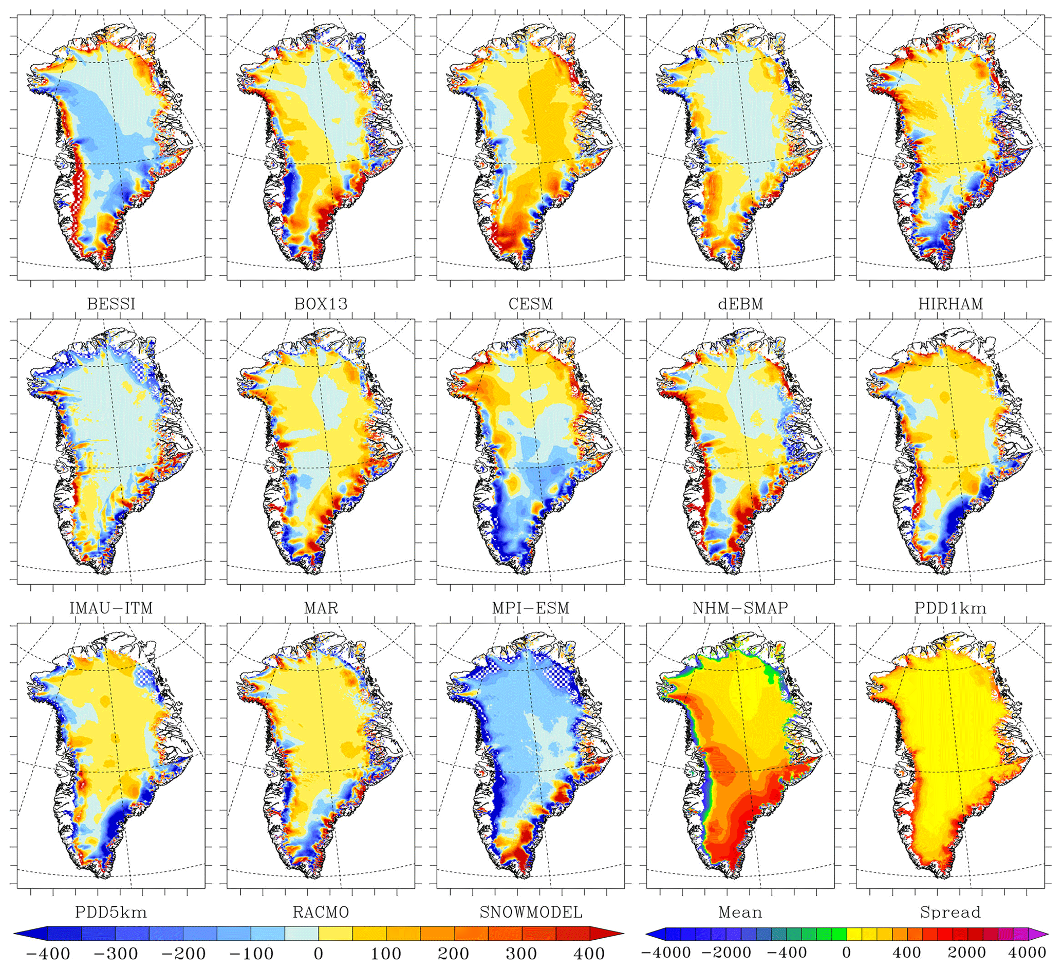
Figure 2Same as Fig. 1 but for the modelled SMB vs. the ensemble model mean over 1980–2012 (shown in the last two plots). As in Fig. 1, the areas listed in Table 4 where SMB disagrees with the MODIS-derived bare ice area are shown in a hatched area.
Integrated over the common main ice sheet mask (see Table 2), the average total GrIS SMB over 1980–2012 ranges from 96 Gt yr−1 (SnowModel) to 429 Gt yr−1 (NHM-SMAP), with a mean value of ∼ 340 ± 110 Gt yr−1. Comparing the two largest SMB components (i.e. snowfall and runoff), we can see large discrepancies between models. For some models, SMB falls within the range of the other models only due to compensating effects of over- or underestimating both snowfall and runoff (see Fig. S1). For example, the snowfall and runoff from BESSI and the PDD models are very low compared to other models but yield similar integrated SMB values. In addition, the SMB of NHM-SMAP (SnowModel) is substantially higher (lower) than that of other models, due to larger snowfall accumulation (meltwater runoff) than other models. Except for SnowModel (which suggests a SMB trend close to −12.9 Gt yr−2) and both GCMs, all models suggest that the SMB of the GrIS has decreased at a rate of ∼ 7 Gt yr−2 over the period 1980–2012, primarily due to an increase in meltwater runoff (∼ +8 Gt yr−2). It is also interesting to note that the meltwater runoff increase is about 2 times lower in the GCMs, probably because a recent increase in atmospheric blocking events in summer, increasing surface runoff, is not captured by the GCMs (Hanna et al., 2018). Finally, while Bougamont et al. (2007) concluded that PDDs are more sensitive to climate warming than the EBMs, it is not the case here as the PDD-based melt rates are fully included in the EBM-based spread, including over the extreme summers (e.g. 2012).
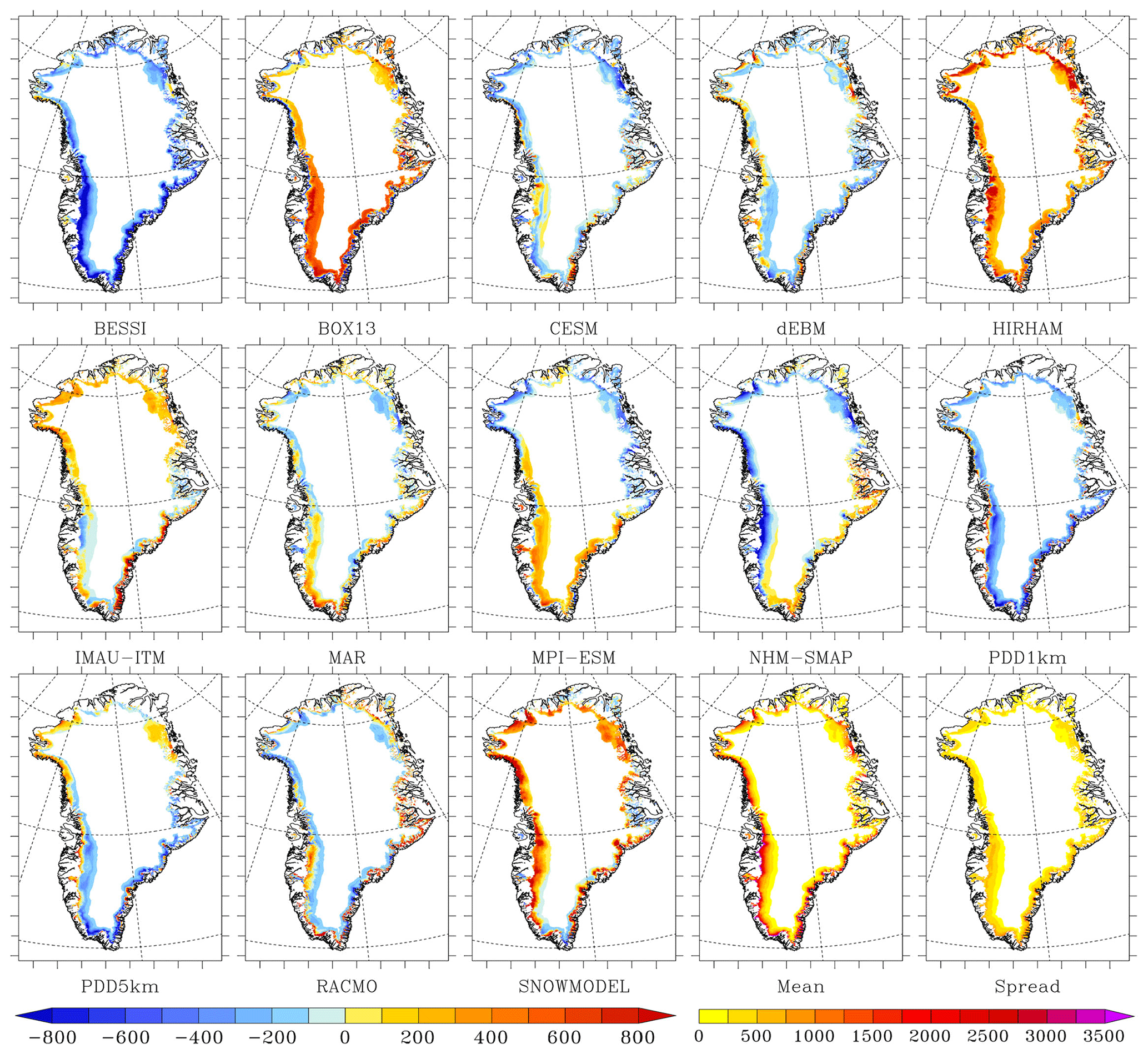
Figure 3Same as Fig. 2 but for the modelled runoff. The ensemble mean and model spread around the mean are also shown in mm w.e. yr−1 in the two last plots. Finally it is important to note that only the area where the runoff of the ensemble mean is higher than 100 mm w.e. yr−1 is shown here.
If we compare each model to the ensemble mean (see Figs. 1 and 2), we can see that BESSI, NHM-SMAP and PDD1km generally simulate lower runoff in the ablation zone compared to the other models (Fig. 3). In contrast, SnowModel, HIRHAM and BOX13 simulate larger runoff than the ensemble mean. These differences largely explain the SMB anomaly in the ablation zone shown in Fig. 2 with respect to the ensemble mean. Finally, IMAU-ITM, BESSI and SnowModel are drier in the interior of the ice sheet (Fig. 4), even though they use identical ERA-Interim precipitation forcing as the other PDD and EBM models.
In the accumulation zone of South Greenland, CESM simulates larger snowfall rates while MPI-ESM simulates small ones in addition to larger runoff than the ensemble mean. Finally, for all the RCMs, the snowfall accumulation does not show similar and systematic deviations over a large extent from the ensemble mean. This better representation of the spatial variability in precipitation in the RCMs is likely due to the fact that the precipitation is resolved at higher resolution than in both the GCMs and the ERA-Interim reanalysis, the latter of which is used to force the PDD and EBM models. This highlights the advantage of simulating precipitation at high spatial resolution in order to represent the interaction between the atmospheric flow and (ice-sheet) topography. The south-east coast of Greenland shows the largest discrepancy between models, reaching 2 m w.e. yr−1 locally, and this is where most RCMs simulate higher precipitation than other types of models. Unfortunately, in situ data coverage along the south-eastern coast is very sparse, making it hard to prove whether high accumulation rates in RCMs, locally exceeding 3 m w.e. yr−1, are actually realistic. This highlights the need for a higher density of in situ measurements in south-east Greenland where the models simulate the maximum precipitation. Shallow ice radar or remote sensing (elevation changes) could also help to evaluate the accumulation rates in this area.
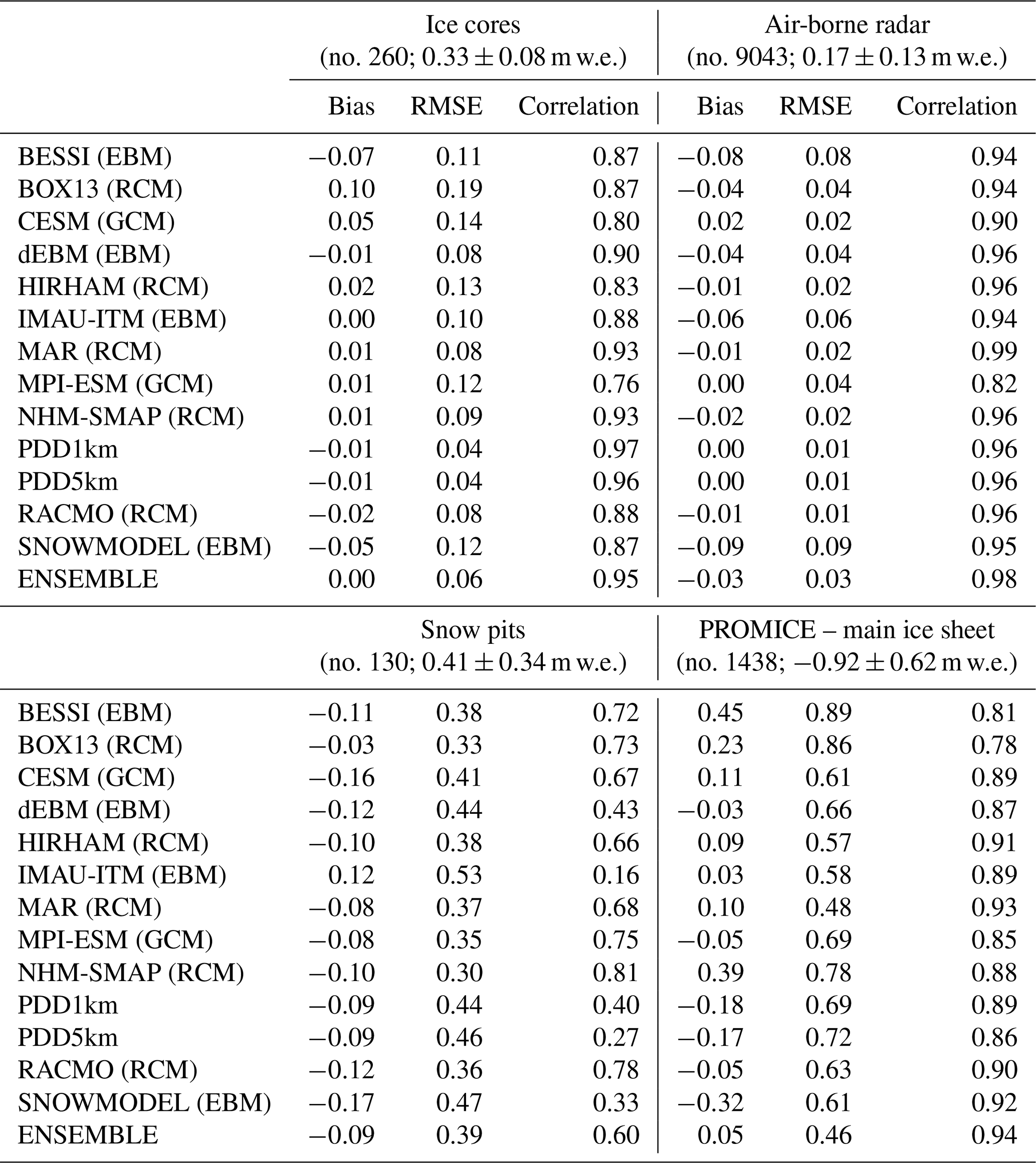
Table 3Statistics (in m w.e.) of models vs. SMB databases described in Sect. 3. The number of measurements as well as the mean value and the standard deviation around this mean value for each data set is listed in the titles of the table. Finally, except for both PDD models, the statistics of models vs. the SMB PROMICE database over the main ice sheet or the peripheral ice caps from the common ice sheet mask are given in Table S1 in the Supplement.
5.1 Comparison with in situ SMB measurements
In comparison with SMB derived from ice cores (location shown in Fig. 5), both PDD models perform the best (see Table 3). However, the same ice core data set has been used to correct ERA-Interim precipitation as that used to force both of these models, and therefore they are not completely independent. Furthermore, the RCMs MAR, NHM-SMAP and RACMO2.3 generally agree better with observations than the other models that use ERA-Interim precipitation as forcing or GCM-based precipitation computed at lower spatial resolution. Except for the two PDD models, the RMSE of the models is generally larger than the standard deviation of the ice core measurements, meaning that the model biases are statistically significant.
In comparison with airborne radar transects, all the models compare very well and biases are not significant but these transects are representative of only a small part of the dry snow zone, already covered by some ice core measurements. Finally, as for the ice cores, the best comparison occurs for the PDD models. We can also note that the correlations are lower for both GCMs as a result of a coarser spatial resolution in GCMs, disallowing the representation of the spatial variability of SMB. However, the RMSE from GCMs is comparable to the other models.
All the models show a worse agreement with the 130 snow pits than with the ice core measurements (Table 3). However, a large part of these discrepancies can likely be ascribed to the use of monthly outputs, with the knowledge that the starting date of the snow pit records (i.e. when the winter accumulation actually started) is uncertain. With respect to the PROMICE SMB data set, the model RMSE varies between 0.48 m w.e. (for MAR) and 0.89 m w.e. (for BESSI) over the main ice sheet. For most of the models, the RMSE is close to the temporal standard deviation (0.62 m w.e.) of the PROMICE data set, suggesting that the modelled biases are not statistically significant. Finally, it is interesting to note that the best statistics are performed with the ensemble mean of the 13 models (see Fig. S1 in supplementary), which will be used hereafter as the SMB reference field. This also suggests that biases of each model are of different signs and are compensated when the 13 model-based estimates are averaged.
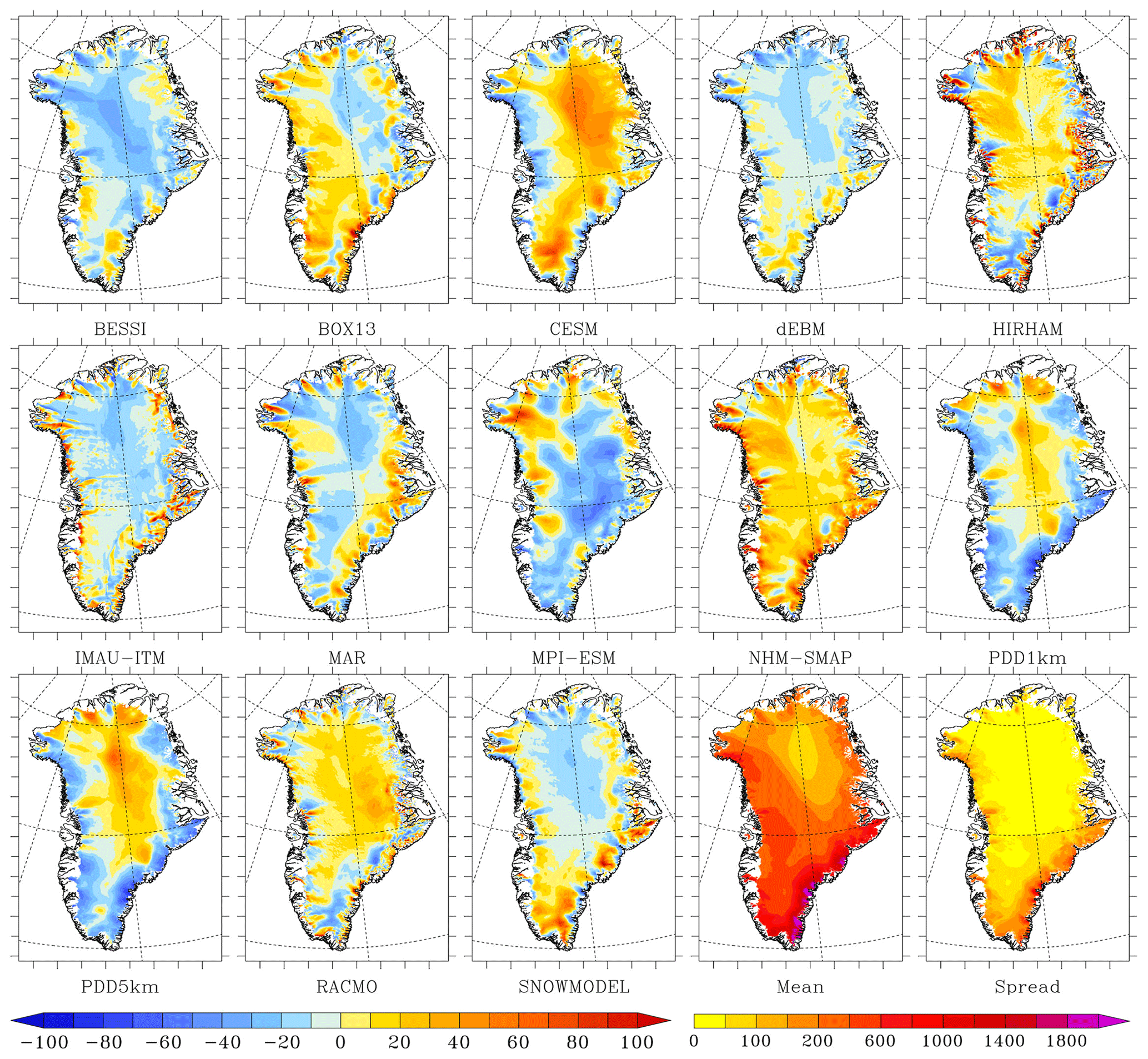
Figure 4Same as Fig. 2 but for the modelled snowfall (linearly interpolated on the 1 km common grid but without any elevation correction) vs. the ensemble model mean over 1980–2012 as a percentage of the ensemble model mean of snowfall accumulation. The ensemble mean and model spread around the mean are also shown in mm w.e. yr−1 in the two last plots.
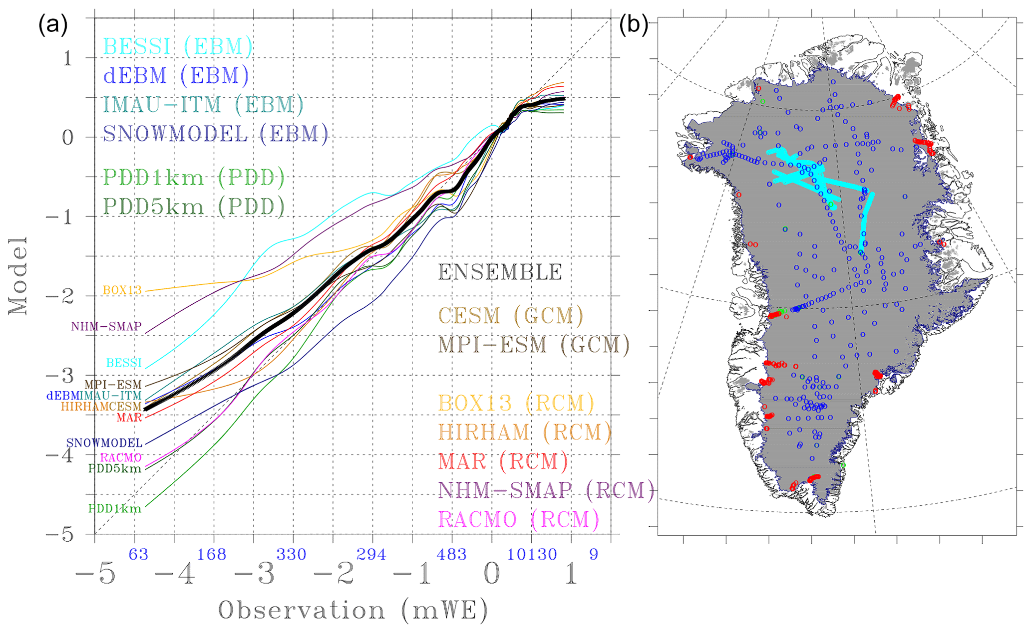
Figure 5(a) Scatter plot of modelled vs. measured SMB in m w.e.. To increase the visibility of this figure, a running mean of 200 samples has been applied here after having sorted the samples (observation, model) on the observations. The numbers in blue on the x axis indicate the number of observations with SMB values within each interval of the x axis. (b) Locations of the in situ measurements: ice cores in dark blue, airborne radar transects in light blue, snow pits in green and PROMICE in red.
In Fig. 5, we can see that all models underestimate most of the few measurements that we have above 1 m w.e. and underestimate ablation rates greater than 3 m w.e., except RACMO2.3 and the two PDD models. Between 0 and 2 m w.e., most of the models rather overestimate ablation. Finally, BESSI, BOX13 and NHM-SMAP systematically underestimate the ablation rates over the whole range of observations, explaining their unfavourable statistics in Table 3 relative to other models.
In brief, it is interesting to note that all types of model generally show similar performance (see Fig. S2). Computationally expensive models (i.e. the RCMs) give the best agreement with observations: MAR and RACMO2.3 perform very well on average compared to SMB observations GrIS-wide, while NHM-SMAP and HIRHAM perform better at representing SMB in the accumulation zone and ablation zone, respectively. However, the evaluation statistics from the more simple models (PDDs and EBMs) and from GCMs are generally similar to those of polar RCMs. It is nevertheless important to note that RCMs were used to calibrate some of these models, partly explaining their general good performance.
Table 4Statistics of models (in which the signal coming from the ice discharge has been subtracted from SMB) vs. GRACE for each basin and the whole ice sheet. The trend (in Gt yr−1) shows the linear trend that must be applied to match GRACE estimates. So negative numbers mean that the downward trend is underestimated compared to GRACE. RMSE (root-mean-square error) and correlation are computed after having applied this trend to the modelled time series.

5.2 Comparison with GRACE measurements
To enable comparison with GRACE mass change, we estimate total mass balance for each model in 6 basins (see Fig. 6 and Table 4) by subtracting observed ice discharge D (King et al., 2018) from modelled SMB for the 13 models, as King et al. (2018) originally did using the RACMO-based SMB:
The GRACE signal variability is mainly a combination of the (i) seasonal cycle (accumulation in winter and melt in summer), (ii) interannual variability in this seasonal cycle and, (iii) long-term climate variability (linked in part to global warming) induced mass loss, which we assume here to be the linear trend over the considered period (2003–2012). Over Basin 1 and 2, IMAU-ITM and SnowModel overestimate and CESM2 and MPI-ESM underestimate the mass loss in the GRACE signal (i.e. the linear trend) over 2003–2012. Over Basin 3, all the models underestimate the mass change. Additionally, some of the models (in particular MAR) do not simulate mass variations in Basin 3, despite GRACE data suggesting a mass loss of 450 Gt over 2003–2012. In south Greenland (Basin 4), the two PDD models show the most favourable statistics but all the models (except MPI-ESM) underestimate mass loss. Along the west coast (Basin 5 and Basin 6), MAR and RACMO2.3 are most closely aligned with the observations, while SnowModel systematically overestimates and NHM-SMAP systematically underestimates the mass loss. For the other models, the bias in Basin 5 and 6 varies in sign. Finally, an EBM (dEBM), a GCM (MPI-ESM), a PDD (PDD1km) and two RCMs (MAR and RACMO2.3) compare the closest to the GRACE-derived GrIS-integrated mass loss over 2003–2012. These favourable statistics are due to error compensation as none of the models matches well with the GRACE-derived regional mass loss integrated over individual basins.
For a total surface mass loss over 2003–2012 of ∼ 3000 Gt as suggested by the GRACE data set, the models range from −1066 to −6034 Gt, with an ensemble mean of −2611 ± 1253 Gt suggesting a large discrepancy between models and therefore a large uncertainty in the modelled SMB trends over the current climate. It is nevertheless interesting to note that, for most of the models, the sign of the bias when compared to the PROMICE data (see Table 3) is highly correlated to the sign of the trend bias with respect to the GRACE-based product. For example, as the 2003–2012 changes in SMB were driven by an increase in melt, those models underestimating surface ablation also underestimate these recent changes (the signal coming from discharge change is the same for all the models). However, we need to mention that all of our modelled total mass balance estimations use the same discharge estimates from King et al. (2018) and do not take into account changes in mass over tundra, over small ice caps (not included in the common ice sheet mask) and in glacial storages (e.g. meltwater lakes, water tables): this partly explains why the discrepancies between models and GRACE could be very high in some areas.
Finally, by removing the linear trend in both time series (i.e. the signal mainly coming from the surface melt increase over 2003–2012 as no change in snowfall accumulation is suggested by the models) we are able to evaluate the seasonal and inter-annual variability gauged here by the RMSE and the correlation listed in Table 4. We find that the five RCMs simulate the seasonal cycle of SMB much better than other types of models (see Fig. S3), although the linear trend over 2003–2012 (Fig. 6) is significantly underestimated, in HIRHAM and NHM-SMAP for example. The two GCMs have a larger RMSE mainly because they are not forced by ERA-Interim, and hence years with high (low) snowfall accumulation (melt) do not necessarily take place at the same time in the GCMs as in the real climate; still, the linear trend over 2003–2012 compares very well with GRACE (e.g. for MPI-ESM).
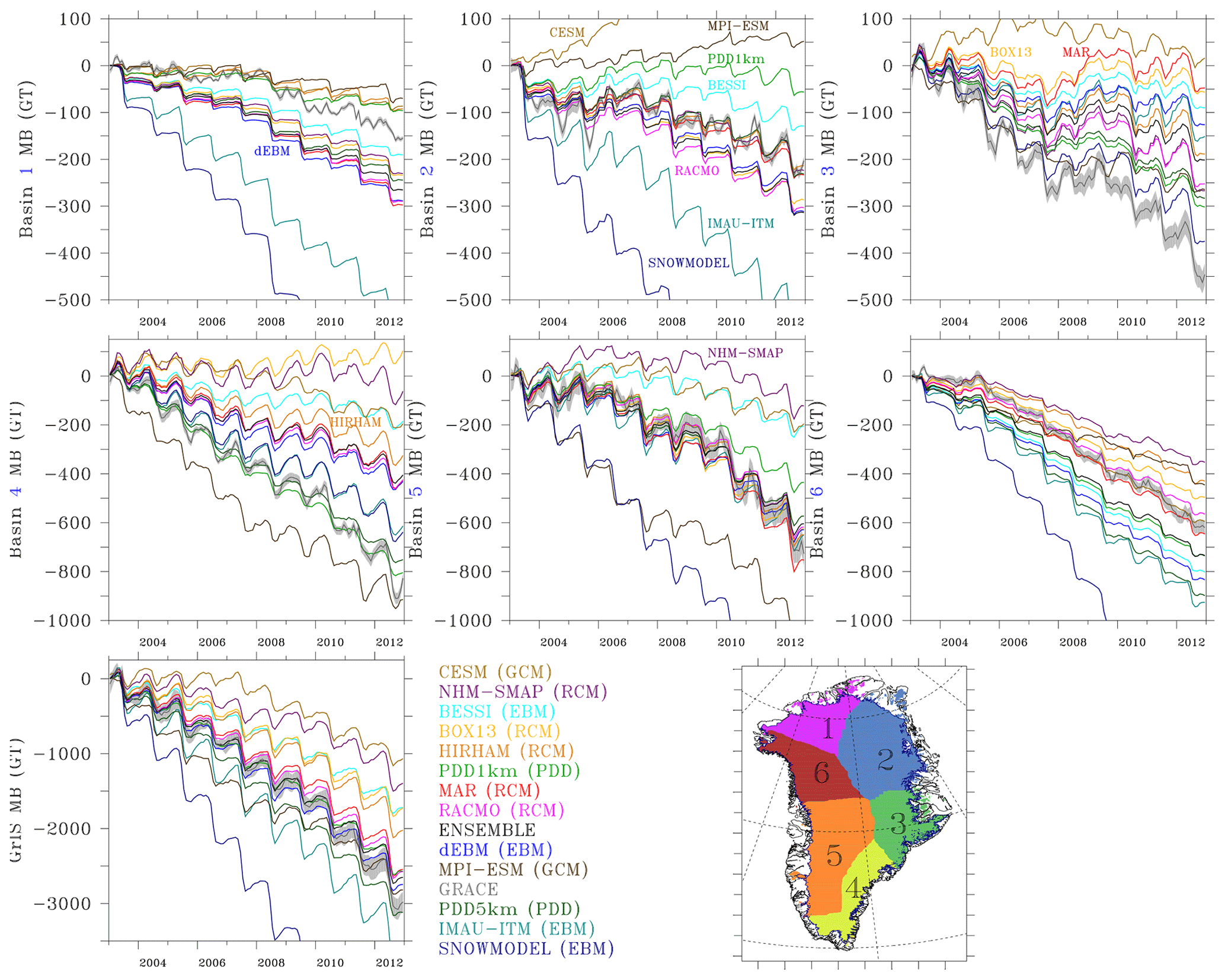
Figure 6Time series of the mass balance (MB) changes from GRACE over 2003–2013 as well as from the 13 models in which the signal from ice discharge (King et al., 2018) has been subtracted from the modelled SMB. Times series are shown for six basins as well as over the whole ice sheet. Except for both PDD models, the ice caps from the common ice sheet mask are included and the tundra areas are discarded. Finally, the legend is sorted in the order of the mass balance changes estimated over the whole ice sheet.
5.3 Comparison with bare ice extent
We can reasonably assume that the mean SMB should be negative in the bare ice area and positive above the snow line. However, the equilibrium line altitude varies each year. Therefore, we have chosen to only use SMB values that fall within 0 mm w.e. yr−1 plus (minus) half of the SMB interannual variability to detect the modelled accumulation (ablation) zone. Apart from BESSI, all models are able to develop a large enough bare ice area, although most of them overestimate the ablation zone extent, in particular IMAU-ITM and SnowModel (see Table 5). In Fig. 1, the hatched areas outline the regions where the models overestimate or underestimate (only for BESSI) the bare ice area. We can see that BESSI fails to represent the extent of the south-western ablation zone. Conversely, IMAU-ITM, BOX13, PDD5km and SnowModel overestimate the extent of the ablation area in north-east Greenland, where the SMB from the other models is also very low but remains positive. Finally, it is interesting to note that both GCMs (CESM2 and MPI-ESM), despite their coarse native resolution in the atmosphere, are able to accurately model the mean snow line, which is attributed to their sub-grid downscaling module.
Table 5Percentage of the main ice sheet area showing the presence of bare ice area detected in MODIS on average over 2000–2012 and where the modelled mean SMB is significantly positive, i.e. where annual SMB is larger than half of the interannual variability (gauged here by the standard deviation). The same is shown for the presence (or lack thereof) of bare ice and where SMB is significantly negative (middle column). The percentage of agreement between modelled ablation zone and bare ice area from MODIS is shown in the right column.

After having inter-compared the models in Sect. 4 and evaluated them with in situ and satellite observations in Sect. 5, this section aims to link the results discussed in the two previous sections. In Fig. 7, we can see that the deviation with the GRACE trend is roughly a linear function of the annual mean GrIS SMB over 1980–2012 and of this trend. The models under- or over-estimating meltwater runoff with respect to the ensemble mean (which compares well with GRACE)systematically under- or over-estimate the GRACE-derived mass loss, largely driven by the increase in meltwater runoff in agreement with the past assessments of SMB seasonal variability using GRACE (Velicogna et al., 2014; Alexander et al., 2016; Schlegel et al., 2016). As the sensitivity of the runoff to temperature increase is not linear (Fettweis et al., 2013a), the runoff increase is smaller and larger for the models under- and over-estimating the meltwater runoff, respectively. With respect to GRACE, the best comparisons occur for mean SMB rates between ∼ 280 and ∼ 380 GT yr−1 over 1980–2012 and SMB trends between and GT yr−2 over 1980–2012. With respect to the PROMICE data set, the best comparisons occur for mean SMB rates and SMB trends, which are between ∼ 280 and ∼ 380 GT yr−1 and between ∼ −9 and ∼ −7 GT yr−2, respectively, over 1980–2012 in agreement with GRACE. According to the linear regression line in Fig. 7, the best mean SMB and SMB trend estimates are ∼ 320 GT yr−1 and ∼ −7.2 GT yr−2, which are very close to the values of the ensemble mean of the 13 models. This suggests that the ensemble mean can be reliably chosen as the best reference to represent the mean SMB and its variability over 1980–2012 for any validation of future model developments.
Except for the two GCMs that underestimate the recent surface mass loss trend mainly because they do not have the same general circulation variability as the ERA-Interim climate, the runoff anomaly expressed in percentage of the ensemble mean remains mainly constant over time, including the extreme summer of 2012. This first confirms that the modelled runoff overestimation and underestimation are systematic over time, independent of the physics used in the model. This also suggests that a runoff bias over the current climate should increase in absolute value for warmer climates in the same proportion as runoff, justifying the importance of representing the current mean climate and trend well before performing future projections.
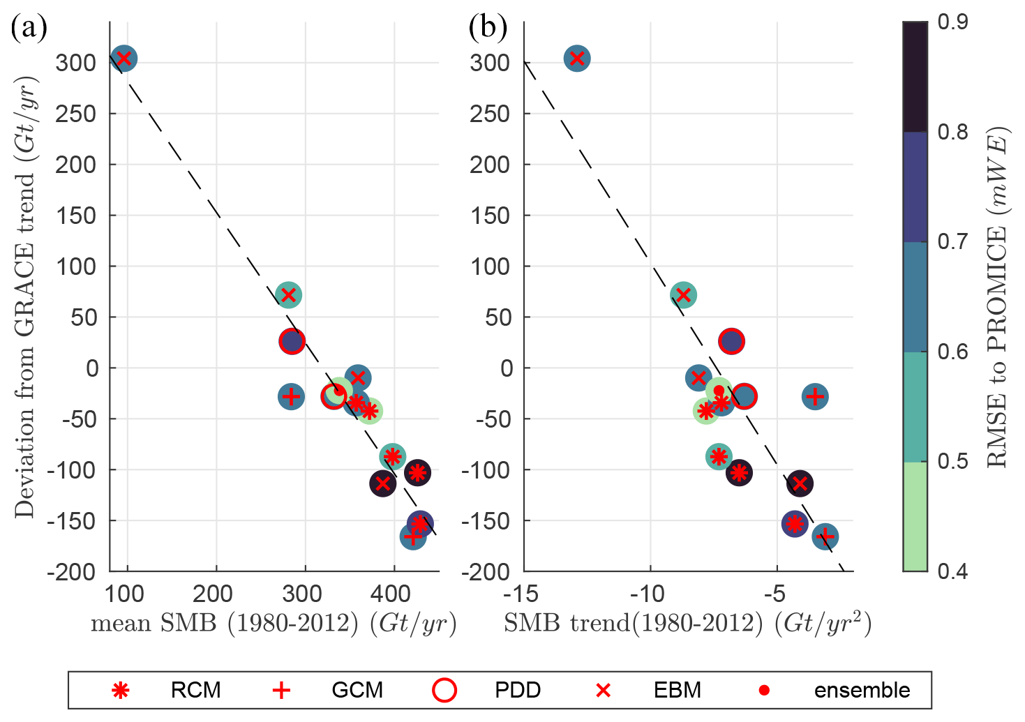
Figure 7(a) Scatter plots of the deviation from GRACE trend (in GT yr−1) vs. mean SMB over 1980–2012 (in GT yr−1), listed in Table 4 and Table 2, respectively. (b) Same as left but with the SMB trend over 1980–2012 (in GT yr−2). In both plots, the background colour indicates the RMSE with the PROMICE SMB database (see Table 3).
Finally, for 95 %, 90 % and 99 % of the 10 767 in situ measurements (see Fig. 1) over the main ice sheet, the mean bias between the ensemble mean and the measurements represents 72 %, 70 % and 75 % of the model spread around this ensemble mean, respectively; it also corresponds to 16 % (resp. 15 % and 18 %) of the observed values. Therefore, we can reasonably estimate three-quarters of the model spread around the ensemble mean as the uncertainty of this ensemble mean-based SMB reconstruction, which gives mean SMB and SMB trend estimates of 338 ± 68 Gt yr−1 and −7.3 ± 2 Gt yr−2 respectively over 1980–2012.
This paper describes the methodology and results of the GrIS SMB Model Intercomparison Project (GrSMBMIP): a novel effort that intercompares GrIS SMB fields produced using five RCMs, four EBMs, two PDDs and two GCMs. Model evaluation using ice core data highlights that polar RCMs (in particular MAR and RACMO2.3) have the most accurate representation of SMB in both the GrIS accumulation and ablation zones, but they are also the only ones to have been calibrated to simulate snowfall and melt individually. Biases of other models are nevertheless of the same order of magnitude as those of polar RCMs, which are often used to calibrate these more simple but faster models. The ensemble mean of the 13 inter-compared models best compares with in situ SMB observations and is among the best modelled estimates to represent the GRACE-derived mass loss trend between 2003 and 2012. Our results reveal that the mean GrIS SMB of all 13 models has been positive between 1980 and 2012 with an average of 338 ± 68 Gt yr−1 but has decreased at an average rate of −7.3 ± 2 Gt yr−2, mainly driven by an increase of 8.0 ± 2 Gt yr−2 in meltwater runoff. The uncertainty has been evaluated to be three-quarters of the model spread around the ensemble mean with respect to the in situ SMB measurements. The good performance of the PDD models in the ablation zone suggests that estimating melt from temperature remains valid under the current climate conditions and that the use of more sophisticated energy balance melt schemes can generate larger biases, despite better a priori physics. Finally, the mean (runoff) bias in the ablation zone mostly explains the large discrepancy between models and GRACE-derived mass loss trend in 2003–2012. Moreover, meltwater runoff biases that operate under current climate could strongly impact the models' ability to simulate future melt acceleration as the present-day runoff bias should increase in absolute value in the same proportion as runoff under warmer climates, independently of the physics used in the models. This suggests for example that a model overestimating the runoff during the extreme 2012 summer by a factor of 2 should a priori overestimate the future sea level rise coming from the Greenland Ice Sheet by roughly the same amount, as future SMB changes will mainly be driven by the surface melt increase (Fettweis et al., 2013a).
RCMs have the advantage that they resolve near-surface climate and dynamically downscale the precipitation to higher spatial resolution with respect to their forcing, while PDD and EBM models are fully driven by the near-surface climate of their low-resolution forcing fields. Although the two GCMs used in this study are not (or are only weakly) forced by historical weather, they simulate the melt reasonably well, which can probably be ascribed to sub-grid elevation corrections applied in MPI-ESM and CESM2. However, for precipitation, the native GCM resolution remains too coarse to resolve the spatial variability simulated by RCMs. The spatial variability of precipitation in RCMs is particularly high along the south-east coast of Greenland. However, the paucity of observations prevents us from confirming whether the local high precipitation rates simulated by RCMs, and not captured by lower resolution models, are realistic. Finally, while RCMs are useful tools for evaluating the melt–elevation feedback since they explicitly compute precipitation and melt changes at high resolution on a different ice sheet topography when coupled with an ice sheet model (Le clec'h et al., 2019), running RCMs at a high spatial resolution becomes computationally expensive on timescales beyond one century. This suggests that the PDD-, EBM- and GCM-based approaches may be more suitable for questions that require long simulations (where a coupling with an ice sheet model may be desirable as well), if they well simulate the current climate (in particular melt runoff).
All the modelled data sets presented in this study are available from the authors upon request and without conditions.
The supplement related to this article is available online at: https://doi.org/10.5194/tc-14-3935-2020-supplement.
XF and SH prepared the paper. UKK provided Fig. 7 and the figures in the Supplement. All authors commented on and improved the paper.
The authors declare that they have no conflict of interest.
This article is part of the special issue “The Ice Sheet Model Intercomparison Project for CMIP6 (ISMIP6)”. It is not associated with a conference.
Xavier Fettweis is a Research Associate from the Fonds de la Recherche Scientifique de Belgique (F.R.S.-FNRS). Computational resources used to perform MAR simulations have been provided by the Consortium des Équipements de Calcul Intensif (CÉCI), funded by the F.R.S.FNRS under grant 2.5020.11 and the Tier-1 supercomputer (Zenobe) of the Fédération Wallonie Bruxelles infrastructure funded by the Walloon Region under grant agreement 1117545. Andreas Born and Tobias Zolles acknowledge financial support from the Trond Mohn Foundation. Constantijn J. Berends, Leo van Kampenhout and Heiko Goelzer have received funding from the programme of the Netherlands Earth System Science Centre (NESSC), financially supported by the Dutch Ministry of Education, Culture and Science (OCW) under grant no. 024.002.001. Edward Hanna acknowledges support from the University of Sheffield's Iceberg high-performance computing team, especially Mike Griffiths. Philippe Huybrechts acknowledges support from the iceMOD project funded by the Research Foundation – Flanders (FWO-Vlaanderen). Marie-Luise Kapsch and Florian Ziemen were funded by the German Federal Ministry of Education and Research (BMBF) through the PalMod project under grant no. 01LP1504C and 01LP1502A. Michalea King acknowledges support from the National Aeronautics and Space Administration (grant nos. 80NSSC18K1027 and NNX13AI21A). Part of the funding for Ruth H. Mottram and Peter L. Langen is provided by the Danish State through the National Centre for Climate Research (NCKF). Bert Wouters was funded by NWO VIDI grant 016.Vidi.171.063. Brice Noël was funded by the NWO VENI grant VI.Veni.192.019. Masashi Niwano, Akihiro Hashimoto, Teruo Aoki and Koji Fujita were supported in part by (1) the Japan Society for the Promotion of Science through Grants-in-Aid for Scientific Research numbers JP16H01772, JP15H01733, JP17K12817, JP17KK0017, JP18H03363 and JP18H05054, and (2) the Ministry of the Environment of Japan through the Experimental Research Fund for Global Environmental Research Coordination System. Paul Gierz is funded by the Federal Ministry for Education and Research initiative PalMod: Simulating a Full Glacial Cycle; BMBF grant 01LP1503B (project PalMod1.2). Uta Krebs-Kanzow acknowledges the Helmholtz Climate Initiative REKLIM and the project “Global sea level change since the Mid Holocene: Background trends and climate-ice sheet feedbacks” funded from the Deutsche Forschungsgemeinschaft (DFG) as part of the Special PriorityProgram (SPP)-1889 “Regional Sea Level Change and Society” (SeaLevel). Gerrit Lohmann acknowledges the Alfred Wegener Institute’s research programme PACES2. Finally, we would like to thank the Ice Sheet Mass Balance and Sea Level (ISMASS) group, funded by CliC (Climate and Cryosphere), for sponsoring this study and Nanna Karlsson (from Geological Survey of Denmark and Greenland, Denmark) for providing airborne radar transect measurements.
This research has been supported by F.R.S.-FNRS, the Fonds Wetenschappelijk Onderzoek-Vlaanderen (FWO) under the EOS project no. O0100718F and the European Union's Horizon 2020 research and innovation programme under the PROTECT project no. 869304. This is PROTECT contribution number 3.
This paper was edited by Robin Smith and reviewed by two anonymous referees.
Alexander, P. M., Tedesco, M., Schlegel, N.-J., Luthcke, S. B., Fettweis, X., and Larour, E.: Greenland Ice Sheet seasonal and spatial mass variability from model simulations and GRACE (2003–2012), The Cryosphere, 10, 1259–1277, https://doi.org/10.5194/tc-10-1259-2016, 2016.
Amante, C. and Eakins, B.: ETOPO1 1 Arc-Minute Global Relief Model: Procedures, Data Sources and Analysis, https://doi.org/10.7289/V5C8276M, 2009.
Aoki, T., Hachikubo, A., and Mashiro, H.: Effects of snow physical parameters on shortwave broadband albedos, J. Geophys. Res., 108, 4616, https://doi.org/10.1029/2003JD003506, 2003.
Aoki, T., Kuchiki, K., Niwano, M., Kodama, Y., Hosaka, M., and Tanaka, T.: Physically based snow albedo model for calculating broadband albedos and the solar heating profile in snowpack for general circulation models, J. Geophys. Res., 116, D11114, https://doi.org/10.1029/2010JD015507, 2011.
Bales, R. C., McConnell, J. R., Mosley-Thompson, E., and Csatho, B.: Accumulation over the Greenland ice sheet from historical and recent records, J. Geophys. Res., 106, 33813–33825, https://doi.org/10.1029/2001JD900153, 2001.
Bales, R. C., Guo, Q., Shen, D., McConnell, J. R., Du, G., Burkhart, J. F., Spikes, V. B., Hanna, E., and Cappelen, J.: Annual accumulation for Greenland updated using ice core data developed during 2000–2006 and analysis of daily coastal meteorological data, J. Geophys. Res., 114, D06116, https://doi.org/10.1029/2008JD011208, 2009.
Bamber, J. L., Griggs, J. A., Hurkmans, R. T. W. L., Dowdeswell, J. A., Gogineni, S. P., Howat, I., Mouginot, J., Paden, J., Palmer, S., Rignot, E., and Steinhage, D.: A new bed elevation dataset for Greenland, The Cryosphere, 7, 499–510, https://doi.org/10.5194/tc-7-499-2013, 2013.
Beamer, J. P., Hill, D. F., Arendt, A., and Liston, G. E.: High-resolutin modeling of coasta freshwater discharge and glacier mass balance in the Gulf of Alaska watershed, Water Resour. Res., 52, 3888–3909, https://doi.org/10.1002/2015WR018457, 2016.
Berends, C. J., de Boer, B., and van de Wal, R. S. W.: Application of HadCM3@Bristolv1.0 simulations of paleoclimate as forcing for an ice-sheet model, ANICE2.1: set-up and benchmark experiments, Geosci. Model Dev., 11, 4657–4675, https://doi.org/10.5194/gmd-11-4657-2018, 2018.
Bintanja, R., van de Wal, R. S. W., and Oerlemans, J.: Global ice volume variations through the last glacial cycle simulated by a 3-D ice-dynamical model, Quatern. Int., 95–96, 11–23, 2002.
Born, A., Imhof, M. A., and Stocker, T. F.: An efficient surface energy–mass balance model for snow and ice, The Cryosphere, 13, 1529–1546, https://doi.org/10.5194/tc-13-1529-2019, 2019.
Bougamont, M., Bamber, J. L., Ridley, J. K., Gladstone, R. M., Greuell, W., Hanna, E., Payne, A. J., and Rutt, I.: Impact of model physics on estimating the surface mass balance of the Greenland ice sheet, Geophys. Res. Lett., 34, L17501, https://doi.org/10.1029/2007GL030700, 2007.
Box, J. E.: Greenland ice sheet mass balance reconstruction. Part II: Surface mass balance (1840–2010), J. Climate, 26, 6974–6989, https://doi.org/10.1175/JCLI-D-12-00518.1, 2013.
Box, J. E., Fettweis, X., Stroeve, J. C., Tedesco, M., Hall, D. K., and Steffen, K.: Greenland ice sheet albedo feedback: thermodynamics and atmospheric drivers, The Cryosphere, 6, 821–839, https://doi.org/10.5194/tc-6-821-2012, 2012.
Braithwaite, R. J.: Calculation of sensible-heat flux over a melting ice surface using simple climate data and daily measurements of ablation, Ann. Glaciol., 50, 9–15, https://doi.org/10.3189/172756409787769726, 2009.
Cappelen, J.: DMI monthly climate data collection 1768– 2010, Denmark, the Faroe Islands and Greenland, Danish Meteorological Institute Tech. Rep. 11-05, 54 pp., 2011.
Cappelen, J., Jørgensen, B. V., Laursen, E. V., Stannius, L. S., and Thomsen, R. S.: The observed climate of Greenland, 1958–99 with climatological standard normals, 1961–90, Danish Meteorological Institute Tech. Rep. 00-18, 152 pp., 2001.
Cappelen, J., Laursen, E. V., Jørgensen, P. V., and Kern-Hansen, C.: DMI monthly climate data collection 1768–2005, Denmark, the Faroe Islands and Greenland, Danish Meteorological Institute Tech. Rep. 06-09, 53 pp., 2006.
de Boer, B., Stocchi, P., and van de Wal, R. S. W.: A fully coupled 3-D ice-sheet–sea-level model: algorithm and applications, Geosci. Model Dev., 7, 2141–2156, https://doi.org/10.5194/gmd-7-2141-2014, 2014.
Dee, D. P., Uppala, S. M., Simmons, A. J., Berrisford, P., Poli, P., Kobayashi, S., Andrae, U., Balmaseda, M. A., Balsamo, G., Bauer, P., Bechtold, P., Beljaars, A. C. M., van de Berg, I., Biblot, J., Bormann, N., Delsol, C., Dragani, R., Fuentes, M., Greer, A. J., Haimberger, L., Healy, S. B., Hersbach, H., Holm, E. V., Isaksen, L., Kallberg, P., Kohler, M., Matricardi, M., McNally, A. P., Mong-Sanz, B. M., Morcette, J.-J., Park, B.-K., Peubey, C., de Rosnay, P., Tavolato, C., Thepaut, J. N., and Vitart, F.: The ERA-Interim reanalysis: Configuration and performance of the data assimilation system, Q. J. Roy. Meteorol. Soc., 137, 553–597, https://doi.org/10.1002/qj.828, 2011.
Delhasse, A., Fettweis, X., Kittel, C., Amory, C., and Agosta, C.: Brief communication: Impact of the recent atmospheric circulation change in summer on the future surface mass balance of the Greenland Ice Sheet, The Cryosphere, 12, 3409–3418, https://doi.org/10.5194/tc-12-3409-2018, 2018.
Delhasse, A., Kittel, C., Amory, C., Hofer, S., van As, D., S. Fausto, R., and Fettweis, X.: Brief communication: Evaluation of the near-surface climate in ERA5 over the Greenland Ice Sheet, The Cryosphere, 14, 957–965, https://doi.org/10.5194/tc-14-957-2020, 2020.
ECWMF-IFS: Part IV : Physical Processes (CY33R1), Tech. Rep. June, 2008.
Ekholm, S.: A full coverage, high-resolution, topographic model of Greenland computed from a variety of digital elevation data. J. Geophys. Res. 101, 21961-21972, 1996.
Enderlin, E. M., Howat, I. M., Jeong, S., Noh, M.‐J., van Angelen, J. H., and van den Broeke, M. R.: An improved mass budget for the Greenland ice sheet, Geophys. Res. Lett., 41, 866–872, https://doi.org/10.1002/2013GL059010, 2014.
Ettema, J., van den Broeke, M. R., van Meijgaard, E., van de Berg, W. J., Box, J. E., and Steffen, K.: Climate of the Greenland ice sheet using a high-resolution climate model – Part 1: Evaluation, The Cryosphere, 4, 511–527, https://doi.org/10.5194/tc-4-511-2010, 2010.
Fettweis, X., Franco, B., Tedesco, M., van Angelen, J. H., Lenaerts, J. T. M., van den Broeke, M. R., and Gallée, H.: Estimating the Greenland ice sheet surface mass balance contribution to future sea level rise using the regional atmospheric climate model MAR, The Cryosphere, 7, 469–489, https://doi.org/10.5194/tc-7-469-2013, 2013a.
Fettweis, X., Hanna, E., Lang, C., Belleflamme, A., Erpicum, M., and Gallée, H.: Brief communication ”Important role of the mid-tropospheric atmospheric circulation in the recent surface melt increase over the Greenland ice sheet”, The Cryosphere, 7, 241–248, https://doi.org/10.5194/tc-7-241-2013, 2013b.
Fettweis, X., Box, J. E., Agosta, C., Amory, C., Kittel, C., Lang, C., van As, D., Machguth, H., and Gallée, H.: Reconstructions of the 1900–2015 Greenland ice sheet surface mass balance using the regional climate MAR model, The Cryosphere, 11, 1015–1033, https://doi.org/10.5194/tc-11-1015-2017, 2017.
Franco, B., Fettweis, X., Lang, C., and Erpicum, M.: Impact of spatial resolution on the modelling of the Greenland ice sheet surface mass balance between 1990–2010, using the regional climate model MAR, The Cryosphere, 6, 695–711, https://doi.org/10.5194/tc-6-695-2012, 2012.
Gates, W. L., Boyle, J., Covey, C., Dease, C., Doutriaux, C., Drach, R., Fiorino, M., Gleckler, P., Hnilo, J., Marlais, S., Phillips, T., Potter, G., Santer, B., Sperber, K., Taylor, K., and Williams, D.: An Overview of the Results of the Atmospheric Model Intercomparison Project (AMIP I), B. Am. Meteor. Soc., 73, 1962–1970, 1998.
Gates, W. L., Boyle, J., Covey, C., Dease, C., Doutriaux, C., Drach, R., Fiorino, M., Gleckler, P., Hnilo, J., Marlais, S., Phillips, T., Potter, G., Santer, B., Sperber, K., Taylor, K., and Williams, D.: An Overview of the Results of the Atmospheric Model Intercomparison Project (AMIP I), B. Am. Meteorol. Soc., 80, 29–56, https://doi.org/10.1175/1520-0477(1999)080<0029:AOOTRO>2.0.CO;2, 1999
Goelzer, H., Huybrechts, P., Furst, J., Nick, F., Andersen, M., Eswards, T., Fettweis, X., Payne, A., and Shannon, S.: Sensitivity of Greenland ice sheet projections to model formulations, J. Glaciol., 59, 733–749, 2013.
Greuell, W.: Numerical Modelling of the Energy Balance and the Englacial Temperature at the ETH Camp, West Greenland, Zürcher Geographische Schriften, 51, 1–81, 1992.
Hahn, L. C., Storelvmo, T., Hofer, S., Parfitt, R., and Ummenhofer, C. C.: Importance of orography for Greenland cloud and melt response to atmospheric blocking, J. Climate, 33, 4187–4206, https://doi.org/10.1175/JCLI-D-19-0527.1, 2020.
Hanna, E., Huybrechts, P., Janssens, I., Cappelen, J., Steffen, K., and Stephens, A.: Runoff and mass balance of the Greenland ice sheet: 1958–2003, J. Geophys. Res., 110, D13108, https://doi.org/10.1029/2004JD005641, 2005.
Hanna, E., Huybrechts, P., Cappelen, J., Steffen, K., Bales, R. C., Burgess, E., McConnell, J. R., Steffensen, J. P., Van den Broeke, M., Wake, L., Bigg, G., Griffiths, M., and Savas, D.: Greenland Ice Sheet surface mass balance 1870 to 2010 based on Twentieth Century Reanalysis, and links with global climate forcing, J. Geophys. Res., 116, D24121, https://doi.org/10.1029/2011JD016387, 2011.
Hanna, E., Fettweis, X., and Hall, R. J.: Brief communication: Recent changes in summer Greenland blocking captured by none of the CMIP5 models, The Cryosphere, 12, 3287–3292, https://doi.org/10.5194/tc-12-3287-2018, 2018.
Hanna, E., Pattyn, F., Navarro, F., Favier, V., Goelzer, H., van den Broeke, M. R., Vizcaino, M., Whitehouse, P. L., Ritz, C., and Bulthuis, K. and Smith, B.: Mass balance of the ice sheets and glaciers – progress since AR5 and challenges, Earth Sci. Rev., 201, 102976, https://doi.org/10.1016/j.earscirev.2019.102976, 2020.
Hashimoto, A., Niwano, M., Aoki, T., Tsutaki, S., Sugiyama, S., Yamasaki, T., Iizuka, Y., and Matoba, S.: Numerical weather prediction system based on JMA-NHM for field observation campaigns on the Greenland ice sheet, Low Temperature Science, 75, 91–104, https://doi.org/10.14943/lowtemsci.75.91, 2017.
Hofer, S., Tedstone, A. J., Fettweis, X., and Bamber, J.: Cloud microphysics and circulation anomalies control differences in future Greenland melt, Nat. Clim. Chang., 9, 523–528, https://doi.org/10.1038/s41558-019-0507-8, 2019.
Hofer, S., Tedstone, A. J., Fettweis, X., and Bamber, J. L.: Decreasing cloud cover drives the recent mass loss on the Greenland Ice Sheet, Sci. Adv., 3, e170058, https://doi.org/10.1126/sciadv.1700584, 2017.
Howat, I. M., Negrete, A., and Smith, B. E.: The Greenland Ice Mapping Project (GIMP) land classification and surface elevation data sets, The Cryosphere, 8, 1509–1518, https://doi.org/10.5194/tc-8-1509-2014, 2014.
Hurrell, J. W., Hack, J. J., Shea, D., Caron, J. M., and Rosinski J.: A New Sea Surface Temperature and Sea Ice Boundary Dataset for the Community Atmosphere Model, J. Climate, 21, 5145–5153, https://doi.org/10.1175/2008JCLI2292.1, 2008.
Huybrechts, P. and de Wolde, J.: The Dynamic Response of the Greenland and Antarctic Ice Sheets to Multiple-Century Climatic Warming, J. Climate, 12, 2169–2188, 1999.
IMBIE2: Mass balance of the Greenland Ice Sheet from 1992 to 2018, Nature, 579, 233–239, https://doi.org/10.1038/s41586-019-1855-2, 2020.
IPCC: Summary for Policymakers, in: IPCC Special Report on the Ocean and Cryosphere in a Changing Climate, edited by: Pörtner, H.-O., Roberts, D. C., Masson-Delmotte, V., Zhai, P., Tignor, M., Poloczanska, E., Mintenbeck, K., Nicolai, M., Okem, A., Petzold, J., Rama, B., and Weyer, N., in press, 2019.
Janssens, I. and Huybrechts, P.: The treatment of meltwater retention in mass-balance parameterizations of the Greenland ice sheet, Ann. Glaciol., 31, 133–140, 2000.
Jowett, A. E., Hanna, E., Ng, F., Huybrechts, P., and Janssens, I.: A new spatially and temporally variable sigma parameter in degree-day melt modelling of the Greenland Ice Sheet 1870–2013, The Cryosphere Discuss., 9, 5327–5371, https://doi.org/10.5194/tcd-9-5327-2015, 2015.
Karlsson, N. B., Eisen, O., Dahl-Jensen, D., Freitag, J., Kipfstuhl, S., Lewis, C., Nielsen, L. T., Paden, J. D., Winter, A., and Wilhelms, F.: Accumulation Rates during 1311–2011 CE in North-Central Greenland Derived from Air-Borne Radar Data, Front. Earth Sci., 4, 97, https://doi.org/10.3389/feart.2016.00097, 2016.
Karlsson, N. B., Razik, S., Hörhold, M., Winter, A., Steinhage, D., Binder, T., and Eisen, O.: Surface Accumulation in Northern Central Greenland during the last 300 Years, Ann. Glaciol., 61, 214–224, https://doi.org/10.1017/aog.2020.30, 2020.
Khan, S. A., Sasgen, I., Bevis, M., van Dam, T., Bamber, J. L., Wahr, J., Willis, M., Kjaer, K. H., Wouters, B., Helm, V., Csatho, B., Fleming, K., Bjork, A. A., Aschwanden, A., Knudsen, P., and Munneke, P. K.: Geodetic measurements reveal similarities between post-Last Glacial Maximum and present-day mass loss from the Greenland ice sheet, Sci. Adv., 2, e1600931, https://doi.org/10.1126/sciadv.1600931, 2016.
King, M. D., Howat, I. M., Jeong, S., Noh, M. J., Wouters, B., Noël, B., and van den Broeke, M. R.: Seasonal to decadal variability in ice discharge from the Greenland Ice Sheet, The Cryosphere, 12, 3813–3825, https://doi.org/10.5194/tc-12-3813-2018, 2018.
Kobayashi, S., Ota, Y., Harada, Y., Ebita, A., Moriya, M., Onoda, H., Onogi, K., Kamahori, H., Kobayashi, C., Endo, H., Miyaoka, K., and Takahashi, K.: The JRA-55 reanalysis: General specifications and basic characteristics, J. Meteorol. Soc. Jpn., 93, 5–48, https://doi.org/10.2151/jmsj.2015-001, 2015.
Krebs-Kanzow, U., Gierz, P., and Lohmann, G.: Brief communication: An ice surface melt scheme including the diurnal cycle of solar radiation, The Cryosphere, 12, 3923–3930, https://doi.org/10.5194/tc-12-3923-2018, 2018.
Krebs-Kanzow, U., Gierz, P., Rodehacke, C. B., Xu, S., Yang, H., and Lohmann, G.: The diurnal Energy Balance Model (dEBM): A convenient surface mass balance solution for ice sheets in Earth System modeling, The Cryosphere Discuss., https://doi.org/10.5194/tc-2020-247, in review, 2020.
Langen, P. L., Fausto, R. S., Vandecrux, B., Mottram R. H., and Box, J. E.: Liquid Water Flow and Retention on the Greenland Ice Sheet in the Regional Climate Model HIRHAM5: Local and Large-Scale Impacts, Front. Earth Sci., 4, 110, https://doi.org/10.3389/feart.2016.00110, 2017.
Le clec'h, S., Charbit, S., Quiquet, A., Fettweis, X., Dumas, C., Kageyama, M., Wyard, C., and Ritz, C.: Assessment of the Greenland ice sheet–atmosphere feedbacks for the next century with a regional atmospheric model coupled to an ice sheet model, The Cryosphere, 13, 373–395, https://doi.org/10.5194/tc-13-373-2019, 2019.
Lenaerts, J. T. M., van den Broeke, M. R., van Angelen, J. H., van Meijgaard, E., and Déry, S. J.: Drifting snow climate of the Greenland ice sheet: a study with a regional climate model, The Cryosphere, 6, 891–899, https://doi.org/10.5194/tc-6-891-2012, 2012.
Lenaerts, J. T. M., Medley, B., van den Broeke, M. R., and Wouters, B.: Observing and modeling ice sheet surface mass balance, Rev. Geophys., 57, 376–420, https://doi.org/10.1029/2018RG000622, 2019.
Lewis, G., Osterberg, E., Hawley, R., Whitmore, B., Marshall, H. P., and Box, J.: Regional Greenland accumulation variability from Operation IceBridge airborne accumulation radar, The Cryosphere, 11, 773–788, https://doi.org/10.5194/tc-11-773-2017, 2017.
Lewis, G., Osterberg, E., Hawley, R., Marshall, H. P., Meehan, T., Graeter, K., McCarthy, F., Overly, T., Thundercloud, Z., and Ferris, D.: Recent precipitation decrease across the western Greenland ice sheet percolation zone, The Cryosphere, 13, 2797–2815, https://doi.org/10.5194/tc-13-2797-2019, 2019.
Ligtenberg, S. R. M., Kuipers Munneke, P., Noël, B. P. Y., and van den Broeke, M. R.: Brief communication: Improved simulation of the present-day Greenland firn layer (1960–2016), The Cryosphere, 12, 1643–1649, https://doi.org/10.5194/tc-12-1643-2018, 2018.
Liston, G. E.: Local advection of momentum, heat, and moisture during the melt of patchy snow covers, J. Appl. Meteorol., 34, 1705–1715, https://doi.org/10.1175/1520-0450-34.7.1705, 1995.
Liston, G. E. and Elder, K.: A distributed snow-evolution modeling system (SnowModel), J. Hydrometeorol., 7, 1259–1276, https://doi.org/10.1175/JHM548.1, 2006a.
Liston, G. E. and Elder, K.: A meteorological distribution system for high-resolution terrestrial modeling (MicroMet). J. Hydrometeorol., 7, 217–234, https://doi.org/10.1175/JHM486.1, 2006b.
Liston, G. E. and Hiemstra, C. A.: The changing cryosphere: pan-Arctic snow trends (1979–2009), J. Clim., 24, 5691–5712, 2011.
Liston, G. E. and Mernild, S. H.: Greenland freshwater runoff. Part I: a runoff routing model for glaciated and non-glaciated landscapes (HydroFlow), J. Clim., 25, 5997–6014, https://doi.org/10.1029/2011JD016267, 2012.
Liston, G. E. and Sturm, M.: A snow-transport model for complex terrain, J. Glaciol., 44, 498–516, 1998.
Liston, G. E. and Sturm, M.: Winter precipitation patterns in Arctic Alaska determined from a blowing-snow model and snow depth observations, J. Hydrometeorol., 3, 646–659, 2002.
Liston, G. E., Winther, J.-G., Bruland, O., Elvehøy, H., and Sand, K.: Below surface ice melt on the coastal Antarctic ice sheet, J. Glaciol., 45, 273–285, 1999.
Liston, G. E., Haehnel, R. B., Sturm, M., Hiemstra, C. A., Berezovskaya, S., and Tabler, R. D.: Simulating complex snow distributions in windy environments using SnowTran-3D, J. Glaciol., 53, 241–256, 2007.
Machguth, H., Thomsen, H. H., Weidick, A., Abermann, J., Ahlström, A. P., Andersen, M. L., Andersen, S. B., Björk, A. A., Box, J. E., Braithwaite, R. J., Bøggild, C. E., Citterio, M., Clement, P., Colgan, W., Fausto, R. S., Gleie, K., Hasholt, B., Hynek, B., Knudsen, N. T., Larsen, S. H., Mernild, S., Oerlemans, J., Oerter, H., Olesen, O. B., Smeets, C. J. P. P., Steffen, K., Stober, M., Sugiyama, S., van As, D., van den Broeke, M. R., and van de Wal, R. S.: Greenland surface mass balance observations from the ice sheet ablation area and local glaciers, J. Glaciol., 62, 861–887, https://doi.org/10.1017/jog.2016.75, 2016.
Mauritsen, T., Bader, J., Becker, T., Behrens, J., Bittner, M., Brokopf, R., Brovkin, V., Claussen, M., Crueger, T., Esch, M., Fast, I., Fiedler, S., Fläschner, D., Gayler, V., Giorgetta, M., Goll, DS, Haak, H., Hagemann, S., Hedemann, C., Hohenegger, C., Ilyina, T., Jahns, T., Jimenez de la Cuesta Otero, D., Jungclaus, J., Kleinen, T., Kloster, S., Kracher, D., Kinne, S., Kleberg, D., Lasslop, G., Kornblueh, L., Marotzke, J., Matei, D., Meraner, K., Mikolajewicz, U., Modali , K., Möbis, B., Müller, WA, Nabel, J., Nam, C., Notz, D., Nyawira, S.-S., Paulsen, H., Peters, K., Pincus, R., Pohlmann, H., Pongratz, J., Popp, M., Raddatz, T., Rast, S., Redler, R., Reick, C., Rohrschneider, T., Schemann, V., Schmidt, H., Schnur, R.,Schulzweida, U., Six, K., Stein, L., Stemmler, I., Stevens, B., von Storch, J.-S., Tian, F., Voigt, A., de Vrese, P., Wieners, K.-H., Wilkenskjeld, S., Winkler, A., and Roeckner, E.: Developments in the MPI-M Earth System Model version 1.2 (MPI-ESM1.2) and its response to increasing CO2, J. Adv. Model. Earth Sy., 11, 998– 1038, https://doi.org/10.1029/2018MS001400, 2019.
Mernild, S. H., Liston, G. E., Hasholt, B., and Knudsen, N. T.: Snow distribution and melt modeling for Mittivakkat Glacier, Ammassalik Island, SE Greenland, J. Hydrometeorol., 7, 808–824, 2006.
Mernild, S. H. and Liston, G. E.: Greenland freshwater runoff. Part II: Distribution and trends, 1960–2010, J. Climate, 25, 6015–6035, https://doi.org/10.1175/JCLI-D-11-00592.1, 2012.
Mernild, S. H., Holland, D. M., Holland, D., Rosing-Asvid, A., Yde, J. C., Liston, G. E., and Steffen, K.: Freshwater flux and spatiotemporal simulated runoff variability into Ilulissat Icefjord, West Greenland, linked to salinity and temperature observations near tidewater glacier margins obtained using instrumented ringed seals, J. Phys. Oceanogr., 45, 1426–1445, https://doi.org/10.1175/JPO-D-14-0217.1, 2015.
Morlighem, M., Williams, C. N., Rignot, E., An, L., Arndt, J. E., Bamber, J. L., Catania, G., Chauché, N., Dowdeswell, J. A., Dorschel, B., Fenty, I., Hogan, K., Howat, I. M., Hubbard, A., Jakobsson, M., Jordan, T. M., Kjeldsen, K. K., Millan, R., Mayer, L., Mouginot, J., Noël, B. P. Y., O'Cofaigh, C., Palmer, S., Rysgaard, S., Seroussi, H., Siegert, M. J., Slabon, P., Straneo, F., van den Broeke, M. R., Weinrebe, W., Wood, M., and Zinglersen, K. B.: BedMachine v3: Complete Bed Topography and Ocean Bathymetry Mapping of Greenland From Multibeam Echo Sounding Combined With Mass Conservation, Geophys. Res. Lett., 44, 11051–11061, 2017.
Mouginot, J., Rignot, E., Bjørk, A., van den Broeke, M., Millan, R., Morlighem, M., Noël, B., Scheuchl, B., and Wood, M.: Forty-six years of Greenland Ice Sheet mass balance from 1972 to 2018, P. Natl. Acad. Sci. USA, 116, 9239–9244, https://doi.org/10.1073/pnas.1904242116, 2019.
Müller, W. A., Jungclaus, J. H., Mauritsen, T., Baehr, J., Bittner, M., Budich, R., Bunzel, F., Esch, M., Ghosh, R., Haak, H., Ilyina, T., Kleine, T., Kornblueh, L., Li, H., Modali, K., Notz, D., Pohlmann, H., Roeckner, E., Stemmler, I., Tian, F., and Marotzke J.: A higher-resolution version of the Max Planck Institute Earth System Model (MPI-ESM1.2-HR), J. Adv. Model. Earth Sy., 10, 1383–1413, 2018.
Niwano, M., Aoki, T., Kuchiki, K., Hosaka, M., Kodama, Y., Yamaguchi, S., Motoyoshi, H., and Iwata, Y.: Evaluation of updated physical snowpack model SMAP, Bull. Glaciol. Res., 32, 65–78, https://doi.org/10.5331/bgr.32.65, 2014.
Niwano, M., Aoki, T., Kuchiki, K., Hosaka, M., and Kodama, Y.: Snow Metamorphism and Albedo Process (SMAP) model for climate studies: Model validation using meteorological and snow impurity data measured at Sapporo, Japan, J. Geophys. Res., 117, F03008, https://doi.org/10.1029/2011JF002239, 2012.
Niwano, M., Hashimoto, A., and Aoki, T.: Cloud-driven modulations of Greenland ice sheet surface melt, Sci. Rep., 9, 10380, https://doi.org/10.1038/s41598-019-46152-5, 2019.
Niwano, M., Aoki, T., Hashimoto, A., Matoba, S., Yamaguchi, S., Tanikawa, T., Fujita, K., Tsushima, A., Iizuka, Y., Shimada, R., and Hori, M.: NHM–SMAP: spatially and temporally high-resolution nonhydrostatic atmospheric model coupled with detailed snow process model for Greenland Ice Sheet, The Cryosphere, 12, 635–655, https://doi.org/10.5194/tc-12-635-2018, 2018.
Noël, B., van de Berg, W. J., Machguth, H., Lhermitte, S., Howat, I., Fettweis, X., and van den Broeke, M. R.: A daily, 1 km resolution data set of downscaled Greenland ice sheet surface mass balance (1958–2015), The Cryosphere, 10, 2361–2377, https://doi.org/10.5194/tc-10-2361-2016, 2016.
Noël, B., van de Berg, W. J., van Wessem, J. M., van Meijgaard, E., van As, D., Lenaerts, J. T. M., Lhermitte, S., Kuipers Munneke, P., Smeets, C. J. P. P., van Ulft, L. H., van de Wal, R. S. W., and van den Broeke, M. R.: Modelling the climate and surface mass balance of polar ice sheets using RACMO2 – Part 1: Greenland (1958–2016), The Cryosphere, 12, 811–831, https://doi.org/10.5194/tc-12-811-2018, 2018.
Noël B, van de Berg, W. J., Lhermitte, S., and van den Broeke, M. R.: Rapid ablation zone expansion amplifies north Greenland mass loss, Sci Adv., 5, eaaw0123, https://doi.org/10.1126/sciadv.aaw0123, 2019.
Nowicki, S. M. J., Payne, A., Larour, E., Seroussi, H., Goelzer, H., Lipscomb, W., Gregory, J., Abe-Ouchi, A., and Shepherd, A.: Ice Sheet Model Intercomparison Project (ISMIP6) contribution to CMIP6, Geosci. Model Dev., 9, 4521–4545, https://doi.org/10.5194/gmd-9-4521-2016, 2016.
Oerlemans, J. and Knap, W. H.: A 1 Year Record of Global Radiation and Albedo in the Ablation Zone of Morteratschgletscher, Switzerland, J. Glaciol., 44, 231–38, 1998.
Ohmura, A.: Precipitation, accumulation and mass balance of the Greenland ice sheet, Z. Gletscherkd. Glazialgeol., 35, 1–20, 1999.
Pfeffer, W. T., Meier, M. F., and Illangasekare, T. H.: Retention of Greenland runoff by refreezing: Implications for projected future sea level change, J. Geophys. Res., 96, 22117– 22124, 1991.
Rae, J. G. L., Aðalgeirsdóttir, G., Edwards, T. L., Fettweis, X., Gregory, J. M., Hewitt, H. T., Lowe, J. A., Lucas-Picher, P., Mottram, R. H., Payne, A. J., Ridley, J. K., Shannon, S. R., van de Berg, W. J., van de Wal, R. S. W., and van den Broeke, M. R.: Greenland ice sheet surface mass balance: evaluating simulations and making projections with regional climate models, The Cryosphere, 6, 1275–1294, https://doi.org/10.5194/tc-6-1275-2012, 2012.
Reijmer, C. H., van den Broeke, M. R., Fettweis, X., Ettema, J., and Stap, L. B.: Refreezing on the Greenland ice sheet: a comparison of parameterizations, The Cryosphere, 6, 743–762, https://doi.org/10.5194/tc-6-743-2012, 2012.
Roe, G. H. and Lindzen, R. S.: The Mutual Interaction between Continental-Scale Ice Sheets and Atmospheric Stationary Waves, J. Climate, 14, 1450–1465, 2001.
Roe, G. H.: Modeling precipitation over ice sheets: an assessment using Greenland, Journal of Glaciology 48, 70-80, 2002.
Rolstad, C. and Oerlemans, J.: The residual method for determination of the turbulent exchange coefficient applied to automatic weather station data from Iceland, Switzerland and West Greenland, Ann. Glaciol., 42, 367–372, https://doi.org/10.3189/172756405781813041, 2005.
Ryan, J. C., Smith, L. C., Van As, D., Cooley, S. W., Cooper, M. G., Pitcher, L. H., and Hubbard, A.: Greenland Ice Sheet surface melt amplified by snowline migration and bare ice exposure, Sci. Adv., 5, eaav3738, https://doi.org/10.1126/sciadv.aav3738, 2019.
Saito, K., Fujita, T., Yamada, Y., Ishida, J., Kumagai, Y., Aranami, K., Ohmori, S., Nagasawa, R., Kumagai, S., Muroi, C., Kato, T., Eito, H., and Yamazaki, Y.: The operational JMA nonhydrostatic mesoscale model, Mon. Weather Rev., 134, 1266–1298, https://doi.org/10.1175/MWR3120.1, 2006.
Sasgen, I., van den Broeke, M., Bamber, J. L., Rignot, E., Sørensen, L. S., Wouters, B., Martinec, Z., Velicogna, I., and Simonsen, S. B.: Timing and origin of recent regional ice-mass loss in Greenland, Earth Planet. Sc. Lett., 333–334, 293–303, https://doi.org/10.1016/j.epsl.2012.03.033, 2012.
Schlegel, N.-J., Wiese, D. N., Larour, E. Y., Watkins, M. M., Box, J. E., Fettweis, X., and van den Broeke, M. R.: Application of GRACE to the assessment of model-based estimates of monthly Greenland Ice Sheet mass balance (2003–2012), The Cryosphere, 10, 1965–1989, https://doi.org/10.5194/tc-10-1965-2016, 2016.
Screen, J. A. and Simmonds, I.: The central role of diminishing sea ice in recent Arctic temperature amplification, Nature, 464, 1334–1337, https://doi.org/10.1038/nature09051, 2010.
Simmons, A. J. and Poli, P.: Arctic warming in ERA-Interim and other reanalyses, Q. J. Roy. Meteor. Soc., 141, 1147–1162, https://doi.org/10.1002/qj.2422, 2015.
Steffen, K. and Box J.: Surface climatology of the Greenland ice sheet: Greenland Climate Network 1995–1999, J. Geophys. Res., 106, 33951–33964, 2001.
Tedesco, M. and Fettweis, X.: Unprecedented atmospheric conditions (1948–2019) drive the 2019 exceptional melting season over the Greenland ice sheet, The Cryosphere, 14, 1209–1223, https://doi.org/10.5194/tc-14-1209-2020, 2020.
Undèn, P., Rontu, L., Järvinen, H., Lynch, P., Calvo, J., Cats, G., Cuxart, J., Eerola, K., Fortelius, C., Garcia-Moya, J. A., Jones, C., Lenderlink, G., Mcdonald, A., Mcgrath, R., Navascues, B., Nielsen, N. W., Degaard, V., Rodriguez, E., Rummukainen, M., Sattler, K., Sass, B. H., Savijarvi, H., Schreur, B. W., Sigg, R., The, H., and Tijm, A.: HIRLAM-5, Scientific Documentation, Technical Report, 2002.
Uppala, S. M., Kållberg, P. W., Simmons, A. J., Andrae, U., Da Costa Bechtold, V., Fiorino, M., Gibson, J.K., Haseler, J., Her- nandez, A., Kelly, G. A., Li, X., Onogi, K., Saarinen, S., Sokka, N., Allan, R. P., Anderson, E., Arpe, K., Balmaseda, M. A., Beljaars, A. C. M., Van De Berg, L., Bidlot, J., Bormann, N., Caires, S., Chevallier, F., Dethof, A., Dragosavac, M., Fisher, M., Fuentes, M., Hagemann, S., Hólm, E., Hoskins, B. J., Isaksen, L., Janssen, P. A. E. M., Jenne, R., Mcnally, A. P., Mahfouf, J.-F., Morcrette, J.-J., Rayner, N. A., Saunders, R. W., Simon, P., Sterl, A., Trenbreth, K. E., Untch, A., Vasiljevic, D., Viterbo, P., and Woollen, J.: The ERA-40 re-analysis, Q. J. Roy. Meteor. Soc., 131, 2961–3012, https://doi.org/10.1256/qj.04.176, 2005.
van Angelen, J. H., Lenaerts, J. T. M., Lhermitte, S., Fettweis, X., Kuipers Munneke, P., van den Broeke, M. R., van Meijgaard, E., and Smeets, C. J. P. P.: Sensitivity of Greenland Ice Sheet surface mass balance to surface albedo parameterization: a study with a regional climate model, The Cryosphere, 6, 1175–1186, https://doi.org/10.5194/tc-6-1175-2012, 2012.
van de Berg, W. J. and Medley, B.: Brief Communication: Upper-air relaxation in RACMO2 significantly improves modelled interannual surface mass balance variability in Antarctica, The Cryosphere, 10, 459–463, https://doi.org/10.5194/tc-10-459-2016, 2016.
van den Broeke, M. R., Enderlin, E. M., Howat, I. M., Kuipers Munneke, P., Noël, B. P. Y., van de Berg, W. J., van Meijgaard, E., and Wouters, B.: On the recent contribution of the Greenland ice sheet to sea level change, The Cryosphere, 10, 1933–1946, https://doi.org/10.5194/tc-10-1933-2016, 2016.
van den Broeke, M., Box, J., Fettweis, X., Hanna, E., Noël, B., Tedesco, M., van As, D., van de Berg, W. J., and van Kampenhout, L.: Greenland Ice Sheet Surface Mass Loss: Recent Developments in Observation and Modeling, Curr. Clim. Change Rep., 3, 345–356, https://doi.org/10.1007/s40641-017-0084-8, 2017.
Van de Wal, R.: Mass-balance modelling of the Greenland ice sheet: A comparison of an energy-balance and a degree-day model, Ann. Glaciol., 23, 36–45, https://doi.org/10.3189/S0260305500013239, 1996.
van Kampenhout, L., Lenaerts, J. T. M., Lipscomb, W. H., Lhermitte, S., Noël, B., Vizcaíno, M., Sacks, W. J., and Van den Broeke, M. R.: Present-Day Greenland Ice Sheet Climate and Surface Mass Balance in CESM2, J. Geophys. Res.-Earth Surf., 125, e2019JF005318, https://doi.org/10.1029/2019JF005318, 2020.
Velicogna, I., Sutterley, T. C., and van den Broeke, M. R.: Regional acceleration in ice mass loss from Greenland and Antarctica using GRACE time-variable gravity data, Geophys. Res. Lett., 41, 8130–8137, https://doi.org/10.1002/2014GL061052, 2014.
Vernon, C. L., Bamber, J. L., Box, J. E., van den Broeke, M. R., Fettweis, X., Hanna, E., and Huybrechts, P.: Surface mass balance model intercomparison for the Greenland ice sheet, The Cryosphere, 7, 599–614, https://doi.org/10.5194/tc-7-599-2013, 2013.
Vinther, B. M., Andersen, K. K., Jones, P. D., Briffa, K. R., and Cappelen, J.: Extending Greenland temperature records into the late eighteenth century, J. Geophys. Res., 111, D11105, https://doi.org/10.1029/2005JD006810, 2006.
Vizcaíno, M., Mikolajewicz, U., Jungclaus, J., and Schurgers, G.: Climate modification by future ice sheet changes and consequences for ice sheet mass balance, Clim. Dynam., 34, 301–324, https://doi.org/10.1007/s00382-009-0591-y, 2010.
Wilton, D. J., Jowett, A., Hanna, E., Bigg, G. R., van den Broeke, M., Fettweis, X., and Huybrechts, P.: High resolution (1 km) positive degree-day modelling of Greenland ice sheet surface mass balance, 1870–2012 using reanalysis data, J. Glaciol. 63, 176–193, 2017.
Yamaguchi, S., Watanabe, K., Katsushima, T., Sato, A., and Kumakura, T.: Dependence of the water retention curve of snow on snow characteristics, Ann. Glaciol., 53, 6–12, https://doi.org/10.3189/2012AoG61A001, 2012.
Yang, K., Koike, T., Stackhouse, P., Mikovitz, C., and Cox, S. J.: An assessment of satellite surface radiation products for highlands with Tibet instrumental data, Geophys. Res. Lett., 33, L22403, https://doi.org/10.1029/2006GL027640, 2006.
Zolles, T. and Born, A.: Sensitivity of the Greenland mass and energy balance to uncertainties in key model parameters, The Cryosphere Discuss., https://doi.org/10.5194/tc-2019-251, in review, 2019.