the Creative Commons Attribution 4.0 License.
the Creative Commons Attribution 4.0 License.
 | 05 Nov 2020
DeepBedMap: a deep neural network for resolving the bed topography of Antarctica
To resolve the bed elevation of Antarctica, we present DeepBedMap – a novel machine learning method that can produce Antarctic bed topography with adequate surface roughness from multiple remote sensing data inputs. The super-resolution deep convolutional neural network model is trained on scattered regions in Antarctica where high-resolution (250 m) ground-truth bed elevation grids are available. This model is then used to generate high-resolution bed topography in less surveyed areas. DeepBedMap improves on previous interpolation methods by not restricting itself to a low-spatial-resolution (1000 m) BEDMAP2 raster image as its prior image. It takes in additional high-spatial-resolution datasets, such as ice surface elevation, velocity and snow accumulation, to better inform the bed topography even in the absence of ice thickness data from direct ice-penetrating-radar surveys. The DeepBedMap model is based on an adapted architecture of the Enhanced Super-Resolution Generative Adversarial Network, chosen to minimize per-pixel elevation errors while producing realistic topography. The final product is a four-times-upsampled (250 m) bed elevation model of Antarctica that can be used by glaciologists interested in the subglacial terrain and by ice sheet modellers wanting to run catchment- or continent-scale ice sheet model simulations. We show that DeepBedMap offers a rougher topographic profile compared to the standard bicubically interpolated BEDMAP2 and BedMachine Antarctica and envision it being used where a high-resolution bed elevation model is required.
- Article
(14991 KB) - Full-text XML
- BibTeX
- EndNote


The bed of the Antarctic ice sheet is one of the most challenging surfaces on Earth to map due to the thick layer of ice cover. Knowledge of bed elevation is however essential for estimating the volume of ice currently stored in the ice sheets and for input to the numerical models that are used to estimate the contribution ice sheets are likely to make to sea level in the coming century. The Antarctic ice sheet is estimated to hold a sea level equivalent (SLE) of 57.9 ± 0.9 m (Morlighem et al., 2019). Between 2012 and 2017, the Antarctic ice sheet was losing mass at an average rate of 219 ± 43 Gt yr−1 (0.61 ± 0.12 mm yr−1 SLE), with most of the ice loss attributed to the acceleration, retreat and rapid thinning of major West Antarctic Ice Sheet outlet glaciers (IMBIE, 2018). Bed elevation exerts additional controls on ice flow by routing subglacial water and providing frictional resistance to flow (Siegert et al., 2004). Bed roughness, especially at short wavelengths, exerts a frictional force against the flow of ice, making it an important influence on ice velocity (Bingham et al., 2017; Falcini et al., 2018). The importance of bed elevation has led to major efforts to compile bed elevation models of Antarctica, notably with the BEDMAP1 (Lythe and Vaughan, 2001) and BEDMAP2 (Fretwell et al., 2013) products. A need for a higher-spatial-resolution digital elevation model (DEM) is also apparent, as ice sheet models move to using sub-kilometre grids in order to quantify glacier ice flow dynamics more accurately (Le Brocq et al., 2010; Graham et al., 2017). Finer grids are especially important at the ice sheet's grounding zone on which adaptive mesh refinement schemes have focused (e.g. Cornford et al., 2016), and attention to the bed roughness component is imperative for proper modelling of fast-flowing outlet glaciers (Durand et al., 2011; Nias et al., 2016). Here we address the challenge of producing a high-resolution DEM while preserving a realistic representation of the bed terrain's roughness.
Estimating bed elevation directly from geophysical observations primarily uses ice-penetrating-radar methods (e.g. Robin et al., 1970). Airborne radar methods enable reliable along-track estimates with low uncertainty (around the 1 % level) introduced by imperfect knowledge of the firn and ice velocity structure, with some potential uncertainty introduced by picking the bed return. Radar-derived bed estimates remain limited in their geographic coverage (Fretwell et al., 2013) and are typically anisotropic in their coverage, with higher spatial sampling in the along-track direction than between tracks.
To overcome these limitations, indirect methods of estimating bed elevation have been developed, and these include inverse methods and spatial statistical methods. Inverse methods use surface observations combined with glaciological-process knowledge to determine ice thickness (e.g. van Pelt et al., 2013). A non-linear relationship exists between the thickness of glaciers, ice streams and ice sheets and how they flow (Raymond and Gudmundsson, 2005), meaning one can theoretically use a well-resolved surface to infer bed properties (e.g. Farinotti et al., 2009). Using surface observation inputs, such as the glacier outline, surface digital elevation models, surface mass balance, surface rate of elevation change, and surface ice flow velocity, various models have been tested in the Ice Thickness Models Intercomparison eXperiment (ITMIX; Farinotti et al., 2017) to determine ice thickness (surface elevation minus bed elevation). While significant inter-model uncertainties do exist, they can be mitigated by combining several models in an ensemble to provide a better consensus estimate (Farinotti et al., 2019). On a larger scale, the inverse technique has also been applied to the Greenland (Morlighem et al., 2017) and Antarctic (Morlighem et al., 2019) ice sheets, specifically using the mass conservation approach (Morlighem et al., 2011). Spatial statistical methods seek to derive a higher-spatial-resolution bed by applying the topographical likeness of bed features known to great detail in one area to other regions. For example, the conditional simulation method applied by Goff et al. (2014) is able to resolve both fine-scale roughness and channelized morphology over the complex topography of Thwaites Glacier and make use of the fact that roughness statistics are different between highland and lowland areas. Graham et al. (2017) uses a two-step approach to generate their synthetic high-resolution grid, with the high-frequency roughness component coming from the ICECAP and BEDMAP1 compilation radar point data and the low-frequency component coming from BEDMAP2. Neither method is perfect, and we see all of the above methods as complementary.
We present a deep-neural-network method that is trained on direct ice-penetrating-radar observations over Antarctica and one which has features from both the indirect inverse modelling and spatial statistical methodologies. An artificial neural network, loosely based on biological neural networks, is a system made up of neurons. Each neuron comprises a simple mathematical function that takes an input to produce an output value, and neural networks work by combining many of these neurons together. The term deep neural network is used when there is not a direct function mapping between the input data and final output but two or more layers that are connected to one another (see LeCun et al., 2015, for a review). They are trained using backpropagation, a procedure whereby the weights or parameters of the neurons' connections are adjusted so as to minimize the error between the ground truth and output of the neural network (Rumelhart et al., 1986). Similar work has been done before using artificial neural networks for estimating bed topography (e.g. Clarke et al., 2009; Monnier and Zhu, 2018), but to our knowledge, no-one so far in the glaciological community has attempted to use convolutional neural networks that work in a more spatially aware, 2-dimensional setting. Convolutional neural networks differ from standard artificial neural networks in that they use kernels or filters in place of regular neurons (again, see LeCun et al., 2015, for a review). The techniques we employ are prevalent in the computer vision community, having existed since the 1980s (Fukushima and Miyake, 1982; LeCun et al., 1989) and are commonly used in visual pattern recognition tasks (e.g. Lecun et al., 1998; Krizhevsky et al., 2012). Our main contributions are twofold: we (1) present a high-resolution (250 m) bed elevation map of Antarctica that goes beyond the 1 km resolution of BEDMAP2 (Fretwell et al., 2013) and (2) design a deep convolutional neural network to integrate as many remote sensing datasets as possible which are relevant to estimating Antarctica's bed topography. We name the neural network “DeepBedMap”, and the resulting digital elevation model (DEM) product “DeepBedMap_DEM”.
2.1 Super resolution
Super resolution involves the processing of a low-resolution raster image into a higher-resolution one (Tsai and Huang, 1984). The idea is similar to the work on enhancing regular photographs to look crisper. The problem is especially ill-posed because a specific low-resolution input can correspond to many possible high-resolution outputs, resulting in the development of several different algorithms aimed at solving this challenge (see Nasrollahi and Moeslund, 2014, for a review). One promising approach is to use deep neural networks (LeCun et al., 2015) to learn an end-to-end mapping between the low- and high-resolution images, a method coined the Super-Resolution Convolutional Neural Network (SRCNN; Dong et al., 2014). Since the development of SRCNN, multiple advances have been made to improve the perceptual quality of super-resolution neural networks (see Yang et al., 2019, for a review). One way is to use a better loss function, also known as a cost function. A loss function is a mathematical function that represents the error between the output of the neural network and the ground truth (see also Appendix A). By having an adversarial component in its loss function, the Super-Resolution Generative Adversarial Network (SRGAN; Ledig et al., 2017) manages to produce super-resolution images with finer perceptual details. A generative adversarial network (Goodfellow et al., 2014) consists of two neural networks, a generator and a discriminator. A common analogy used is to treat the generator as an artist that produces imitation paintings and the discriminator as an art critic that determines the authenticity of the paintings. The artist wants to fool the critic into believing its paintings are real, while the critic tries to identify problems with the painting. Over time, the artist or generator model learns to improve itself based on the critic's judgement, producing authentic-looking paintings with high perceptual quality. Perceptual quality is the extent to which an image looks like a valid natural image, usually as judged by a human. In this case, perceptual quality is quantified mathematically by the discriminator or critic taking into account high-level features of an image like contrast, texture, etc. Another way to improve performance is by reconfiguring the neural network's architecture, wherein the layout or building blocks of the neural network are changed. By removing unnecessary model components and adding residual connections (He et al., 2015), an enhanced deep super-resolution network (EDSR; Lim et al., 2017) features a deeper neural network model that has better performance than older models. For the DeepBedMap model, we choose to adapt the Enhanced Super-Resolution Generative Adversarial Network (ESRGAN; Wang et al., 2019) which brings together the ideas mentioned above. This approach produces state-of-the-art perceptual quality and won the 2018 Perceptual Image Restoration and Manipulation Challenge on Super Resolution (Third Region; Blau et al., 2018).
2.2 Network conditioning
Network conditioning means having a neural network process one source of information in the context of other sources (Dumoulin et al., 2018). In a geographic context, conditioning is akin to using not just one layer but also other relevant layers with meaningful links to provide additional information for the task at hand. Many ways exist to insert extra conditional information into a neural network, such as concatenation-based conditioning, conditional biasing, conditional scaling and conditional affine transformations (Dumoulin et al., 2018). We choose to use the concatenation-based conditioning approach, whereby all of the individual raster images are concatenated together channel-wise, much like the individual bands of a multispectral satellite image. This was deemed the most appropriate conditioning method as all the contextual remote sensing datasets are raster grid images and also because this approach aligns with related work in the remote sensing field.
An example similar to this DEM super-resolution problem is the classic problem of pan-sharpening, whereby a blurry low-resolution multispectral image conditioned with a high-resolution panchromatic image can be turned into a high-resolution multispectral image. There is ongoing research into the use of deep convolutional neural networks for pan-sharpening (Masi et al., 2016; Scarpa et al., 2018), sometimes with the incorporation of specific domain knowledge (Yang et al., 2017), all of which show promising improvements over classical image processing methods. More recently, generative adversarial networks (Goodfellow et al., 2014) have been used in the conditional sense for general image-to-image translation tasks (e.g. Isola et al., 2016; Park et al., 2019), and also for producing more realistic pan-sharpened satellite images (Liu et al., 2018). Our DeepBedMap model builds upon these ideas and other related DEM super-resolution work (Xu et al., 2015; Chen et al., 2016), while incorporating extra conditional information specific to the cryospheric domain for resolving the bed elevation of Antarctica.
3.1 Data preparation
Our convolutional neural network model works on 2-D images, so we ensure all the datasets are in a suitable raster grid format. Ground-truth bed elevation points picked from radar surveys (see Table 1) are first compiled together onto a common Antarctic stereographic projection (EPSG:3031) using the WGS84 datum, reprojecting where necessary. These points are then gridded onto a 250 m spatial resolution (pixel-node-registered) grid. We preprocess the points first using Generic Mapping Tools v6.0 (GMT6; Wessel et al., 2019), computing the median elevation for each pixel block in a regular grid. The preprocessed points are then run through an adjustable-tension continuous-curvature spline function with a tension factor set to 0.35 to produce a digital elevation model grid. This grid is further post-processed to mask out pixels that are more than 3 pixels (750 m) from the nearest ground-truth point.
Bingham et al. (2017)Jordan et al. (2010)King (2011)King et al. (2016)Shi et al. (2010)Table 1High-resolution ground-truth datasets from ice-penetrating-radar surveys (collectively labelled as y) used to train the DeepBedMap model. Training site locations can be seen in Fig. 2.
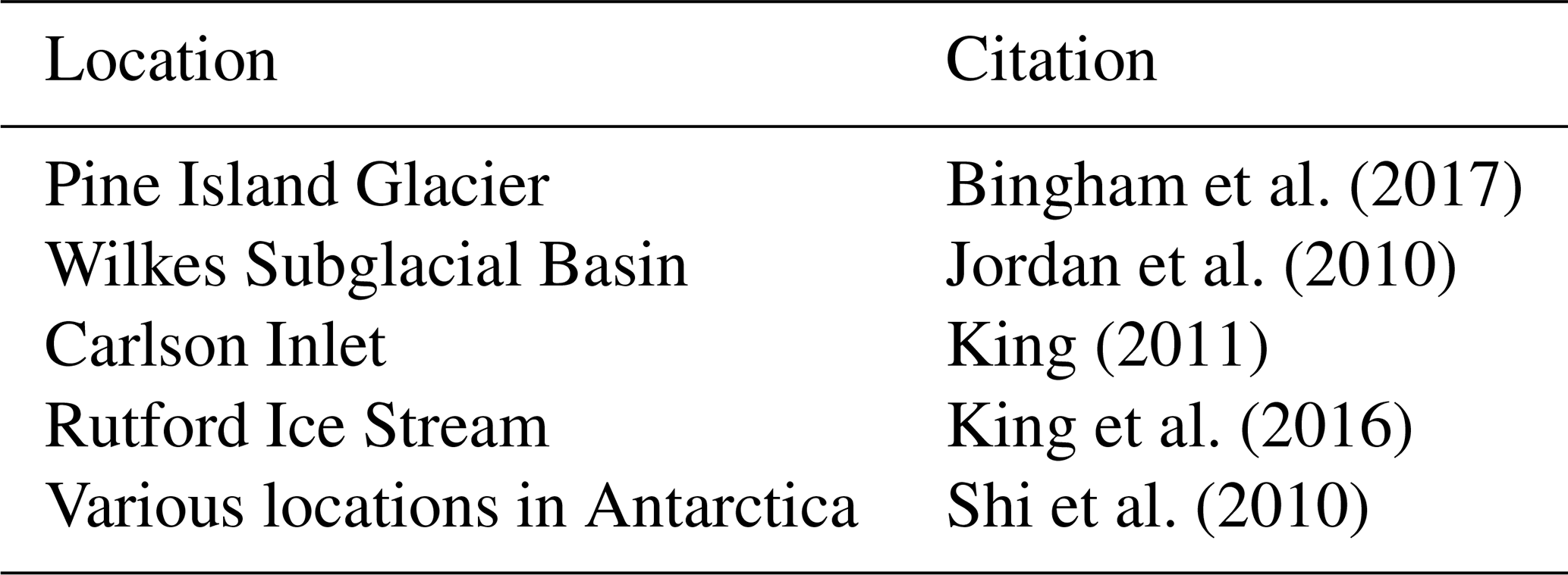
Table 2Remote sensing dataset inputs into the DeepBedMap neural network model.
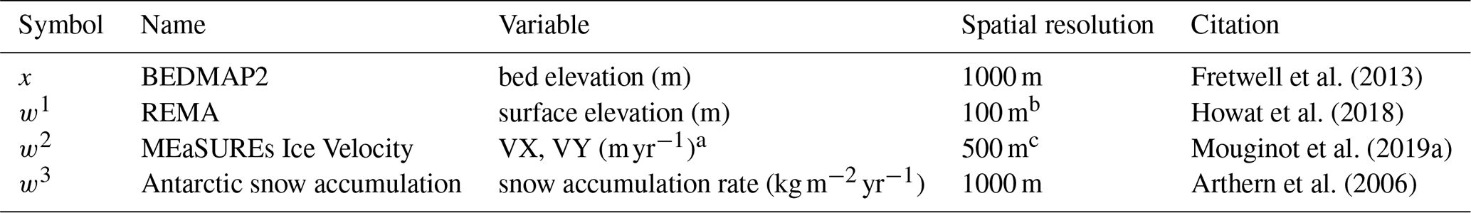
a Note that the x and y components of velocity are used here instead of the norm.
b Gaps in 100 m mosaic filled in with bilinear resampled 200 m resolution REMA image.
c Originally 450 m; bilinear resampled to 500 m.
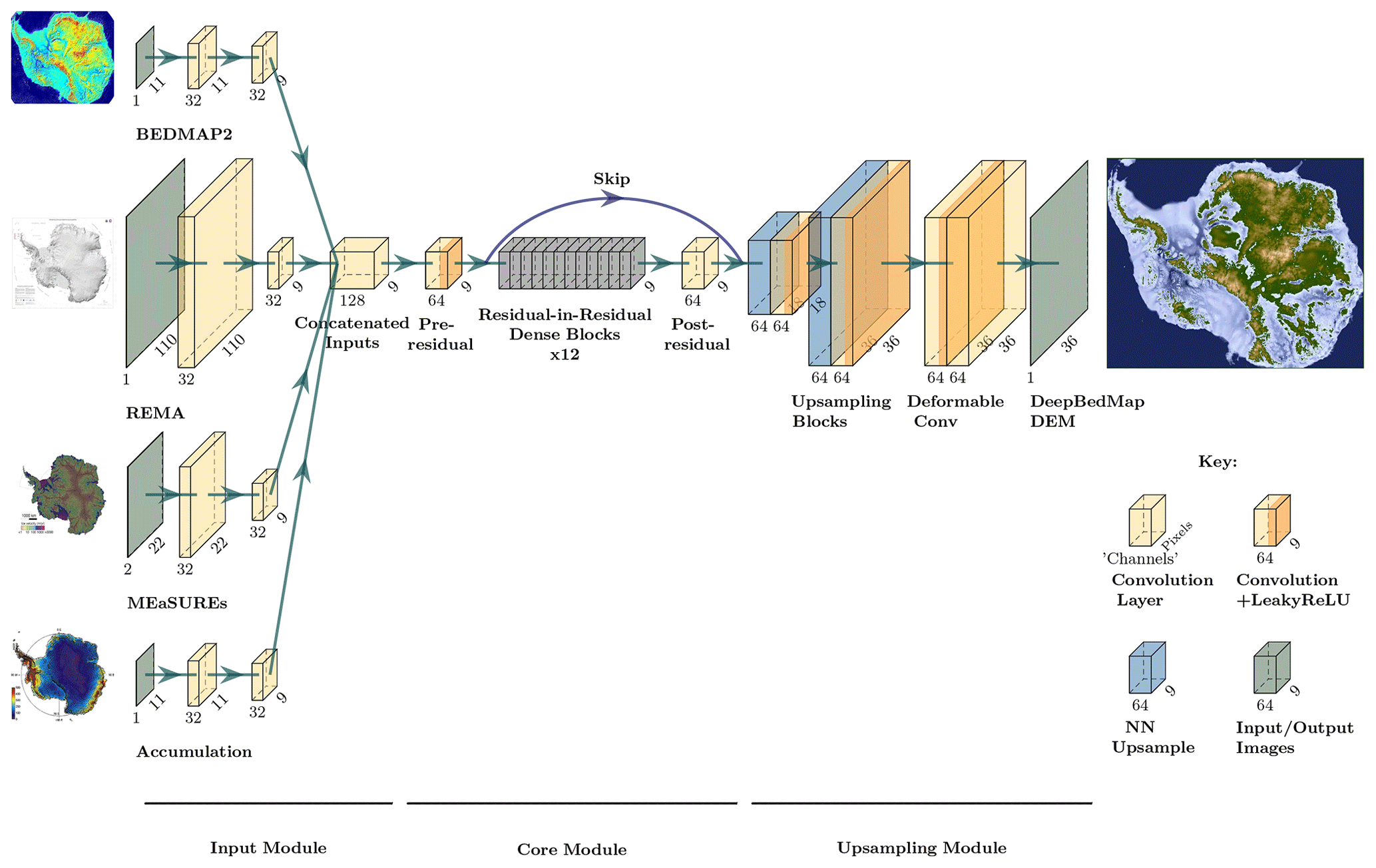
Figure 1DeepBedMap generator model architecture composed of three modules. The input module processes each of the four inputs (BEDMAP2, Fretwell et al., 2013; REMA, Howat et al., 2019; MEaSUREs Ice Velocity, Mouginot et al., 2019b; snow accumulation, Arthern et al., 2006; see also Table 2) into a consistent tensor. The core module processes the rich information contained within the concatenated inputs. The upsampling module scales the tensor up by 4 times and does some extra processing to produce the output DeepBedMap_DEM.
To create the training dataset, we use a sliding window to obtain square tiles cropped from the high-resolution (250 m) ground-truth bed elevation grids, with each tile required to be completely filled with data (i.e. no Not a Number – NaN – values). Besides these ground-truth bed elevation tiles, we also obtain other tiled inputs (see Table 2) corresponding to the same spatial bounding box area. To reduce border edge artefacts in the prediction, the neural network model's input convolutional layers (see Fig. 1) use no padding (also known as “valid” padding) when performing the initial convolution operation. This means that the model input grids (x, w1, w2, w3) have to cover a larger spatial area than the ground-truth grids (y). More specifically, the model inputs cover an area of 11 km × 11 km (e.g. 11 pixels × 11 pixels for BEDMAP2), while the ground-truth grids cover an area of 9 km × 9 km (36 pixels × 36 pixels). As the pixels of the ground-truth grids may not align perfectly with those of the model's input grids, we use bilinear interpolation to ensure that all the input grids cover the same spatial bounds as those of the reference ground-truth tiles. The general locations of these training tiles are shown in orange in Fig. 2.
3.2 Model design
Our DeepBedMap model is a generative adversarial network (Goodfellow et al., 2014) composed of two convolutional neural network models, a generator Gθ that produces the bed elevation prediction and a discriminator Dη critic that will judge the quality of this output. The two models are trained to compete against each other, with the generator trying to produce images that are misclassified as real by the discriminator and the discriminator learning to spot problems with the generator's prediction in relation to the ground truth. Following this is a mathematical definition of the neural network models and their architecture.
The objective of the main super-resolution generator model Gθ is to produce a high-resolution (250 m) grid of Antarctica's bed elevation given a low-resolution (1000 m) BEDMAP2 (Fretwell et al., 2013) image x. However, the information contained in BEDMAP2 is insufficient for this regular super-resolution task, so we provide the neural network with more context through network conditioning (see Sect. 2.2). Specifically, the model is conditioned at the input block stage with three raster grids (see Table 2): (1) ice surface elevation w1, (2) ice surface velocity w2 and (3) snow accumulation w3. This can be formulated as follows:
where Gθ is the generator (see Fig. 1) that produces high-resolution image candidates . For brevity in the following equations, we simplify Eq. (1) to hide conditional inputs w1,w2 and w3, so that all input images are represented using x. To train the generative adversarial network, we update the parameters of the generator θ and discriminator η as follows:
where new estimates of the neural network parameters and are produced by minimizing the total loss functions LG and LD, respectively, for the generator G and discriminator D and and yn are the set of predicted and ground-truth high-resolution images over N training samples. The generator network's loss LG is a custom perceptual loss function with four weighted components – content, adversarial, topographic and structural loss. The discriminator network's loss LD is designed to maximize the likelihood that predicted images are classified as fake (0) and ground-truth images are classified as real (1). Details of these loss functions are described in Appendix A.
Noting that the objective of the generator G is opposite to that of the discriminator D, we formulate the adversarial min–max problem following Goodfellow et al. (2014) as
where for the discriminator D, we maximize the expectation 𝔼 or the likelihood that the probability distribution of the discriminator's output fits D(y)=1 when y∼Pdata(y); i.e. we want the discriminator to classify the high-resolution image as real (1) when the image y is in the distribution of the ground-truth images Pdata(y). For the generator G, we minimize the likelihood that the discriminator classifies the generator output D(G(x))=0 when x∼PG(x); i.e. we do not want the discriminator to classify the super-resolution image as fake (0) when the inputs x are in the distribution of generated images PG(x). The overall goal of the entire network is to make the distribution of generated images G(x) as similar as possible to the ground truth y through optimizing the value function V.
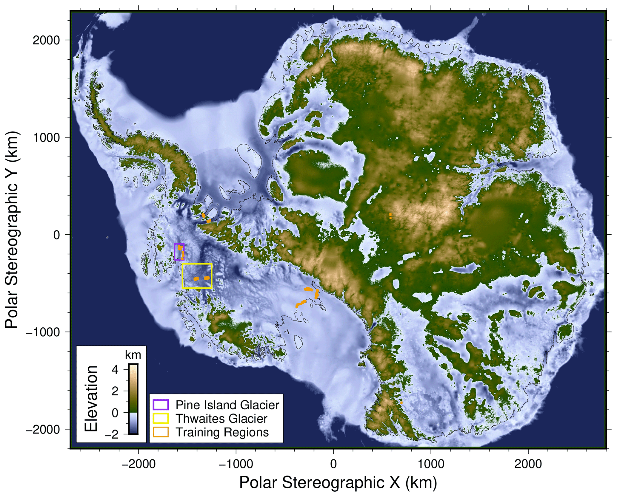
Figure 2DeepBedMap_DEM over the entire Antarctic continent. Plotted on an Antarctic stereographic projection (EPSG:3031) with elevation referenced to the WGS84 datum. Grounding line is plotted as thin black line. Purple box shows Pine Island Glacier extent used in Fig. 3. Yellow box shows Thwaites Glacier extent used in Fig. 5. Orange areas show locations of training tiles (see Table 1).
DeepBedMap's model architecture is adapted from the Enhanced Super-Resolution Generative Adversarial Network (ESRGAN; Wang et al., 2019). The generator model G (see Fig. 1) consists of an input, core and upsampling module. The input module is made up of four sub-networks, each one composed of a convolutional neural network that processes the input image into a consistent 9 × 9 shaped tensor. Note that the MEaSUREs Ice Velocity (Mouginot et al., 2019b) input has two channels, one each for the x and y velocity components. All the processed inputs are then concatenated together channel-wise before being fed into the core module. The core module is based on the ESRGAN architecture with 12 residual-in-residual dense blocks (see Wang et al., 2019, for details), saddled in between a pre-residual and post-residual convolutional layer. A skip connection runs from the pre-residual layer's output to the post-residual layer's output before being fed into the upsampling module. This skip connection (He et al., 2016) helps with the neural network training process by allowing the model to also consider minimally processed information from the input module, instead of solely relying on derived information from the residual-block layers when performing the upsampling. The upsampling module is composed of two upsampling blocks, specifically a nearest-neighbour upsampling followed by a convolutional layer and leaky rectified linear unit (LeakyReLU; Maas et al., 2013) activation, which progressively scales the tensors by 2 times each time. Following this are two deformable convolutional layers (Dai et al., 2017) which produce the final-output super-resolution DeepBedMap_DEM. This generator model is trained to gradually improve its prediction by comparing the predicted output with ground-truth images in the training regions (see Fig. 2), using the total loss function defined in Eq. (A9).
The main differences between the DeepBedMap generator model and ESRGAN are the custom input block at the beginning and the deformable convolutional layers at the end. The custom input block is designed to handle the prior low-resolution BEDMAP2 image and conditional inputs (see Table 2). Deformable convolution was chosen in place of the standard convolution so as to enhance the model's predictive capability by having it learn dense spatial transformations.
Besides the generator model, there is a separate adversarial discriminator model D (not shown in the paper). Again, we follow ESRGAN's (Wang et al., 2019) lead by implementing the adversarial discriminator network in the style of the Visual Geometry Group convolutional neural network model (VGG; Simonyan and Zisserman, 2014). The discriminator model consists of 10 blocks made up of a convolutional, batch normalization (Ioffe and Szegedy, 2015) and LeakyReLU (Maas et al., 2013) layer, followed by two fully connected layers comprised of 100 neurons and 1 neuron, respectively. For numerical stability, we omit the final fully connected layer's sigmoid activation function from the discriminator model's construction, integrating it instead into the binary cross-entropy loss functions at Eqs. (A2) and (A3) using the log-sum-exp function. The output of this discriminator model is a value ranging from 0 (fake) to 1 (real) that scores the generator model's output image. This score is used by both the discriminator and generator in the training process and helps to push the predictions towards more realistic bed elevations. More details of the neural network training setup can be found in Appendix B.
4.1 DeepBedMap_DEM topography
Here we present the output digital elevation model (DEM) of the super-resolution DeepBedMap neural network model and compare it with bed topography produced by other methods. The resulting DEM has a 250 m spatial resolution and therefore a four-times upsampled bed elevation grid product of BEDMAP2 (Fretwell et al., 2013). In Fig. 2, we show that the full Antarctic-wide DeepBedMap_DEM manages to capture general topographical features across the whole continent. The model is only valid for grounded-ice regions, but we have produced predictions extending outside of the grounding-zone area (including ice shelf cavities) using the same bed elevation, surface elevation, ice velocity and snow accumulation inputs where such data are available up to the ice shelf front. We emphasize that the bed elevation under the ice shelves has not been super resolved properly and is not intended for ice sheet modelling use. Users are encouraged to cut the DeepBedMap_DEM using their preferred grounding line (e.g. Bindschadler et al., 2011; Rignot et al., 2011; Mouginot et al., 2017) and replace the under-ice-shelf areas with another bathymetry grid product (e.g. GEBCO Bathymetric Compilation Group, 2020). The transition from the DeepBedMap_DEM to the bathymetry product across the grounding zone can then be smoothed using inverse distance weighting or an alternative interpolation method.
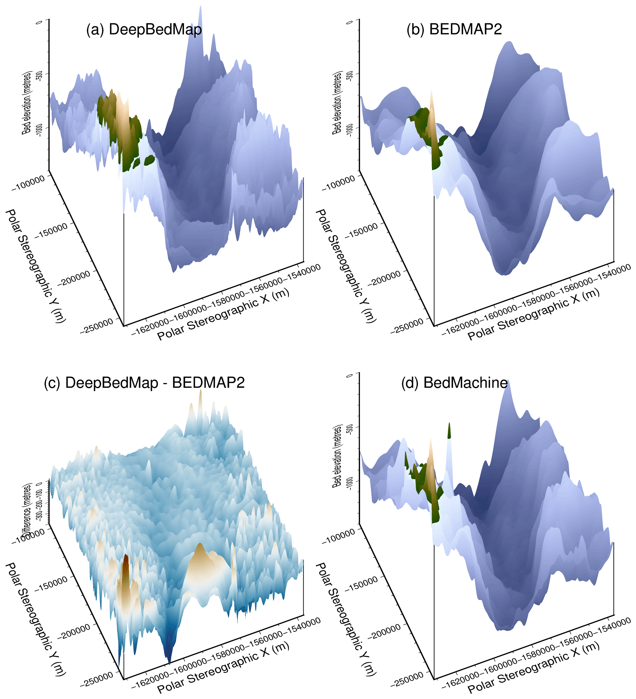
Figure 3Comparison of interpolated bed elevation grid products over Pine Island Glacier (see extent in Fig. 2). (a) DeepBedMap (ours) at 250 m resolution. (b) BEDMAP2 (Fretwell et al., 2013), originally 1000 m, bicubically interpolated to 250 m. (c) Elevation difference between DeepBedMap and BEDMAP2. (d) BedMachine Antarctica (Morlighem, 2019), originally 500 m, bicubically interpolated to 250 m.
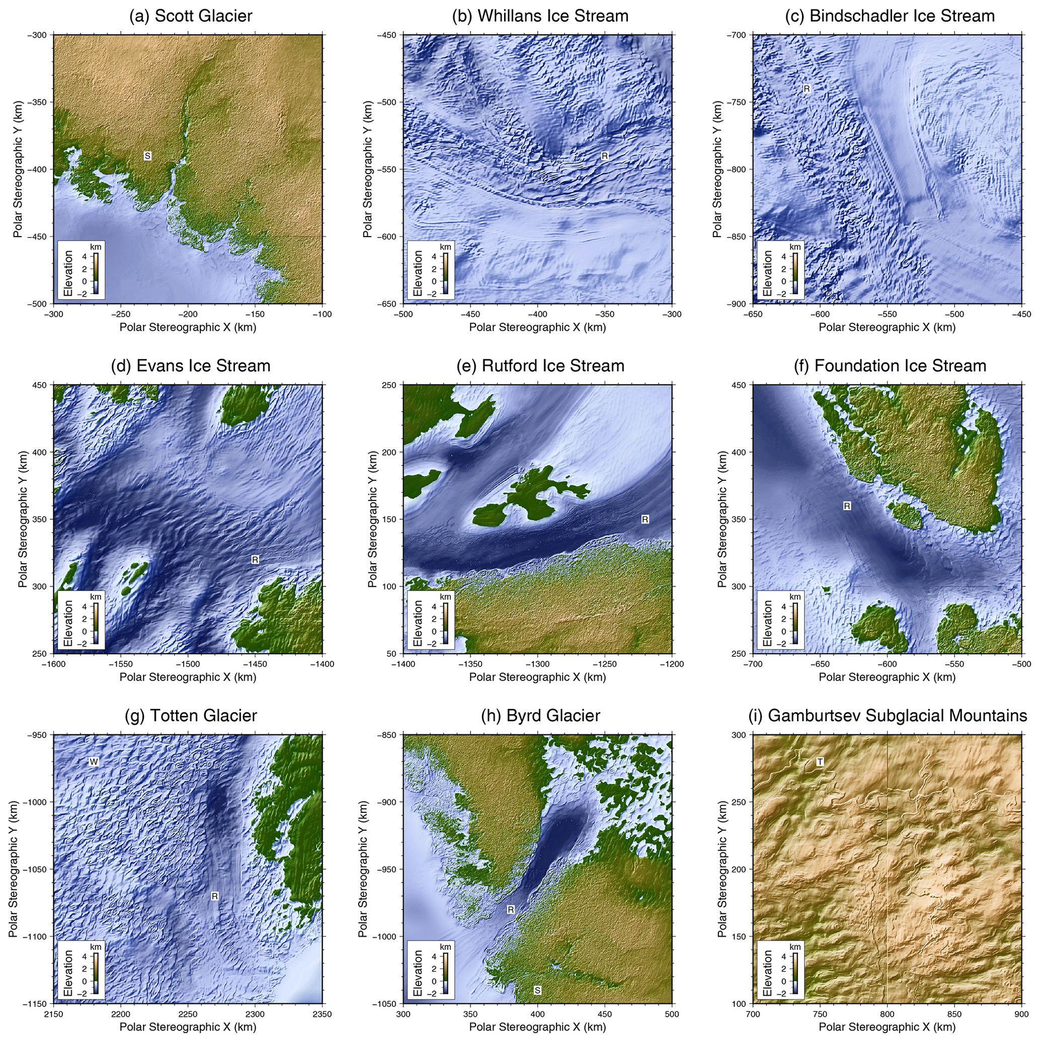
Figure 4Close-up views of DeepBedMap_DEM around Antarctica. Panels (a–c) show Siple Coast locations. Panels (d–f) show Weddell Sea region locations. Panels (g–i) show East Antarctica locations. Features of interest are annotated in black text against a white background: ridges R, speckle patterns S, terraces T, wave patterns W.
We now highlight some qualitative observations of DeepBedMap_DEM's bed topography beneath Pine Island Glacier (Fig. 3) and other parts of Antarctica (Fig. 4). DeepBedMap_DEM shows a terrain with realistic topographical features, having fine-scale bumps and troughs that makes it rougher than that of BEDMAP2 (Fretwell et al., 2013) and BedMachine Antarctica (Morlighem, 2019) while still preserving the general topography of the area (Fig. 3). Over steep topographical areas such as the Transantarctic Mountains (Fig. 4a and h), DeepBedMap produced speckle (S) texture patterns. Along fast-flowing ice streams and glaciers (Fig. 4b–h), we can see ridges (R) aligned parallel to the sides of the valley, i.e. along the flow. In some cases, the ridges are also oriented perpendicularly to the flow direction such as at Whillans Ice Stream (Fig. 4b), Bindschadler Ice Stream (Fig. 4c) and Totten Glacier (Fig. 4g), resulting in intersecting ridges that create a box-like, honeycomb structure. Over relatively flat regions in both West Antarctica and East Antarctica (e.g. Fig. 4g), there are some hummocky, wave-like (W) patterns occasionally represented in the terrain. Terrace (T) features can occasionally be found winding along the side of hills such as at the Gamburtsev Subglacial Mountains (Fig. 4i).
4.2 Surface roughness
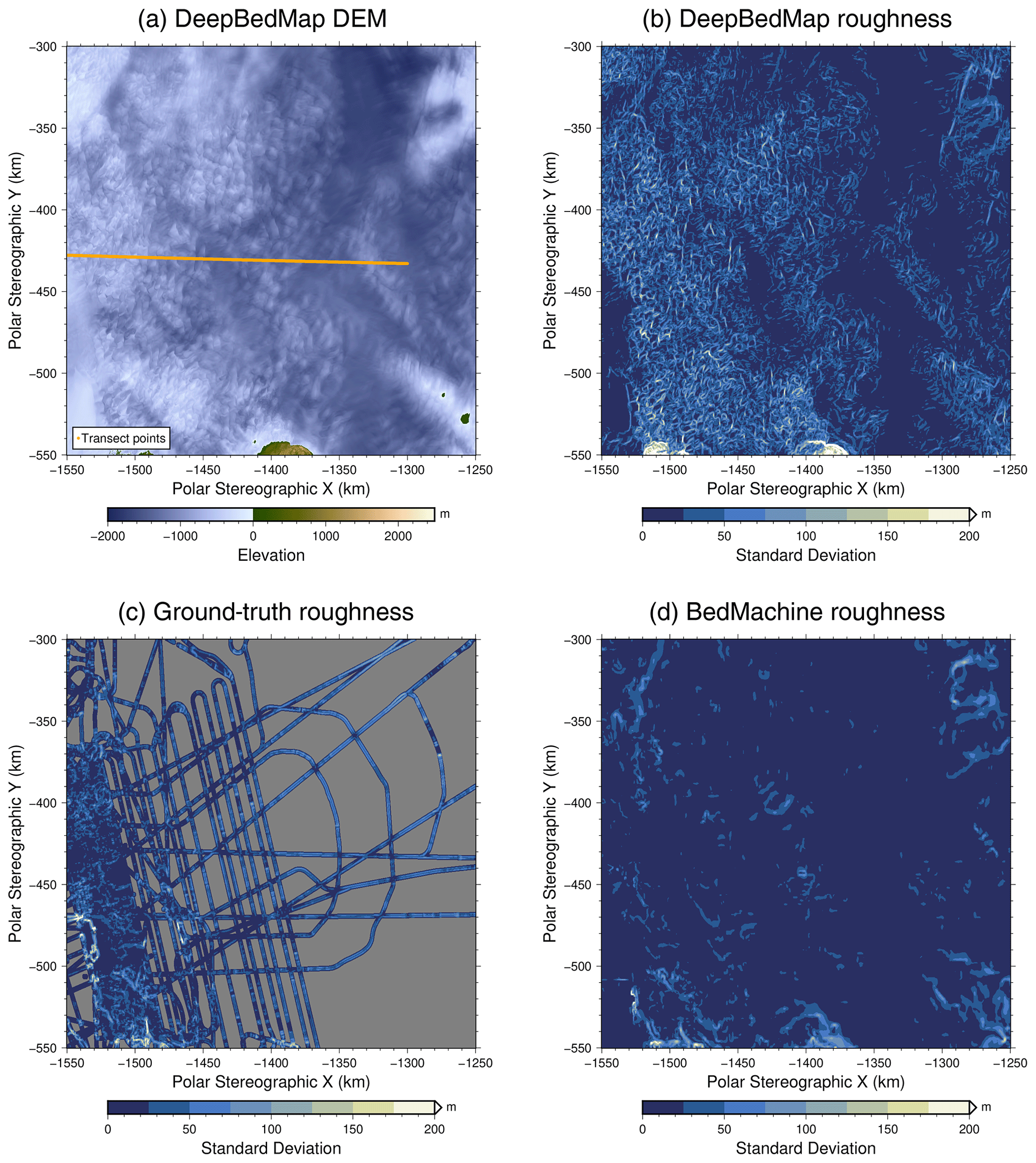
Figure 5Spatial 2-D view of grids over Thwaites Glacier, West Antarctica. Plotted on an Antarctic stereographic projection (EPSG:3031) with elevation and SD values in metres referenced to the WGS84 datum. (a) DeepBedMap digital elevation model. (b) 2-D roughness from the DeepBedMap_DEM grid. (c) 2-D roughness from interpolated Operation IceBridge grid. (d) 2-D roughness from bicubically interpolated BedMachine Antarctica grid. Orange points in (a) correspond to transect sampling locations used in Fig. 6.
We compare the roughness of DeepBedMap_DEM vs. BedMachine Antarctica with ground-truth grids from processed Operation IceBridge data (Shi et al., 2010) using SD as a simple measure of roughness (Rippin et al., 2014). We calculate the surface roughness for a single 250 m pixel from the SD of elevation values over a square 1250 m × 1250 m area (i.e. 5 pixels × 5 pixels) surrounding the central pixel. Focusing on Thwaites Glacier, the spatial 2-D view of the DeepBedMap_DEM (Fig. 5a) shows a range of typical topographic features such as hills and canyons. The calculated 2-D roughnesses for both DeepBedMap_DEM (Fig. 5b) and the Ground truth (Fig. 5c) lie in a similar range from 0 to 400 m, whereas the roughness of BedMachine Antarctica (Fig. 5d) is mostly in the 0-to-200 m range (hence the different colour scale). Also, the roughness pattern for both DeepBedMap_DEM and the ground truth has a more distributed cluster pattern made up of little pockets (especially towards the coastal region on the left; see Fig. 5b and c), whereas the BedMachine Antarctica roughness pattern shows larger cluster pockets in isolated regions (see Fig. 5d).
Taking a 1-D transect over the 250 m resolution DeepBedMap_DEM, BedMachine Antarctica and ground-truth grids, we illustrate the differences in bed topography and roughness from the coast towards the inland area of Thwaites Glacier with a flight trace from Operation IceBridge (see Fig. 6). For better comparison, we have calculated the Operation IceBridge ground-truth bed elevation and roughness values from a resampled 250 m grid instead of using its native along-track resolution. All three elevation profiles are shown to follow the same general trend from the relatively rough coastal region (Fig. 6a from −1550 to −1500 km on the x scale), along the retrograde slope (Fig. 6a from −1500 to −1450 km on the x scale) and into the interior region. DeepBedMap_DEM features a relatively noisy elevation profile with multiple fine-scale (< 10 km) bumps and troughs similar to the ground truth, while BedMachine Antarctica shows a smoother profile that is almost a moving average of the ground-truth elevation (Fig. 6a). Looking at the roughness statistic (Fig. 6b), both the DeepBedMap_DEM and Operation IceBridge ground-truth grids have a mean SD of about 40 m, whereas BedMachine Antarctica has a mean of about 10 m and rarely exceeds a SD value of 20 m along the transect.
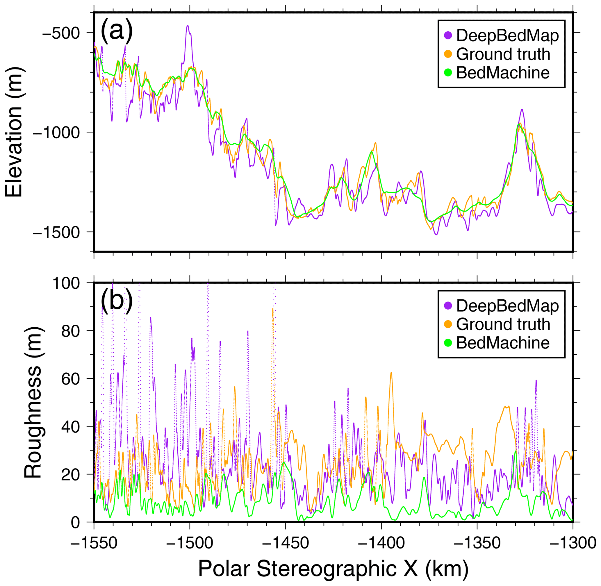
Figure 6Comparing bed elevation (a) and surface roughness (b) (SD of elevation values) of each interpolated grid product (250 m resolution) over a transect (see Fig. 5 for location of transect line). Purple values are from the super-resolution DeepBedMap_DEM; orange values are from tension-spline-interpolated Operation IceBridge ground-truth points; green values are from bicubically interpolated BedMachine Antarctica.
5.1 Bed features
In Sect. 4.1, we show that the DeepBedMap model has produced a high-resolution (250 m) result (see Fig. 3) that can capture a detailed picture of the underlying bed topography. The fine-scale bumps and troughs are the result of the DeepBedMap generator model learning to produce features that are similar to those found in the high-resolution ground-truth datasets it was trained on. However, there are also artefacts produced by the model. For example, the winding terrace (T, Fig. 4) features are hard to explain, and though they resemble eskers (Drews et al., 2017), their placement along the sides of hills does not support this view. Similarly, we are not sure why speckle (S, Fig. 4) texture patterns are found over steep mountains, but the lack of high-resolution training datasets likely leads the model to perform worse over these high-gradient areas.
Another issue is that DeepBedMap will often pick up details from the high-resolution ice surface elevation model (Howat et al., 2019) input dataset, which may not be representative of the true bed topography. For example, the ridges (R, Fig. 4) found along fast-flowing ice streams and glaciers are likely to be the imprints of crevasses or flow stripes (Glasser and Gudmundsson, 2012) observable from the surface. An alternative explanation is that the ridges, especially the honeycomb-shaped ones, are rhombohedral moraine deposits formed by soft sediment squeezed up into basal crevasses that are sometimes found at stagnant surging glaciers (Dowdeswell et al., 2016a, b; Solheim and Pfirman, 1985). We favour the first interpretation as the positions of these bed features coincide with the surface features and also because these ridges are more likely to be eroded away in these fast-flowing ice stream areas.
The hummocky wave-like (W) patterns we observe over the relatively flat and slower-flowing areas are likely to result from surface megadune structures (Scambos, 2014). Alternatively, they may be ribbed or Rogen moraine features that are formed in an orientation transverse to the ice flow direction (Hättestrand, 1997; Hättestrand and Kleman, 1999). While any one of these two explanations may be valid in different regions of Antarctica, we lean towards the conservative interpretation that these features are the result of the DeepBedMap model overfitting to the ice surface elevation data.
5.2 Roughness
In Sect. 4.2, we quantitatively show that a well-trained DeepBedMap neural network model can produce high roughness values more comparable to the ground truth than those of BedMachine Antarctica. While the mass conservation technique used by BedMachine Antarctica (Morlighem et al., 2019) improves upon ordinary interpolation techniques such as bicubic interpolation and kriging, its results are still inherently smooth by nature. The ground-truth grids show that rough areas do exist on a fine scale, and so the high-resolution models we produce should reflect that.
DeepBedMap_DEM manages to capture much of the rough topography found in the Operation IceBridge ground-truth data, especially near the coast (see Fig. 6a, from −1550 to −1500 km on the x scale) where the terrain tends to be rougher. Along the retrograde slope (see Fig. 6a, from −1500 to −1450 km on the x scale), several of the fine-scale (< 10 km) bumps and troughs in DeepBedMap_DEM can be seen to correlate well in position with the ground truth. In contrast, the cubically interpolated BedMachine Antarctica product lacks such fine-scale (< 10 km) bumps and troughs, appearing as a relatively smooth terrain over much of the transect. Previous studies that estimated basal shear stress over Thwaites Glacier have found a band of strong bed extending about 80–100 km from the grounding line, with pockets of weak bed interspersed between bands of strong bed further upstream (Joughin et al., 2009; Sergienko and Hindmarsh, 2013), a pattern that is broadly consistent with the DeepBedMap_DEM roughness results (see Fig. 5b).
In general, DeepBedMap_DEM produces a topography that is rougher, with SD values more in line with those observed in the ground truth (see Fig. 6b). The roughness values for BedMachine Antarctica are consistently lower throughout the transect, a consequence of the mass conservation technique using regularization parameters that yield smooth results. We note that the DeepBedMap_DEM does appear rougher than the ground truth in certain areas. It is possible to tweak the training regime to incorporate roughness (or any statistical measure) into the loss function (see Appendix A) to yield the desired surface, and this will be explored in future work (see Sect. 5.4). Recent studies have stressed the importance of form drag (basal drag due to bed topography) over skin drag (or basal friction) on the basal traction of Pine Island Glacier (Bingham et al., 2017; Kyrke-Smith et al., 2018), and the DeepBedMap super-resolution work here shows strong potential in meeting that demand as a high-resolution bed topography dataset for ice sheet modelling studies.
In terms of bed roughness anisotropy, DeepBedMap is able to capture aspects of it from the ground-truth grids by combining (1) ice flow direction via the ice velocity grid's x and y components (Mouginot et al., 2019b), (2) ice surface aspect via the ice surface elevation grid (Howat et al., 2019), and (3) the low-resolution bed elevation input (Fretwell et al., 2013). There are therefore inherent assumptions that the topography of the current bed is associated with the current ice flow direction, surface aspect and existing low-resolution BEDMAP2 anisotropy. Provided that the direction of this surface velocity and aspect is the same as bed roughness anisotropy, as demonstrated in Holschuh et al. (2020), the neural network will be able to recognize it and perform accordingly. However, if the ice flow direction and surface aspect is not associated with bed anisotropy, then this assumption will be violated and the model will not perform well.
5.3 Limitations
The DeepBedMap model is trained only on a small fraction of the area of Antarctica, at less than 0.1 % of the grounded-ice regions (excluding ice shelves and islands). This is because the pixel-based convolutional neural network cannot be trained on sparse survey point measurements, nor is it able to constrain itself with track-based radar data. As the along-track resolution of radar bed picks are much smaller than 250 m pixels, it is also not easy to preserve roughness from radar unless smaller pixels are used. The topography generated by the model is sensitive to the accuracy of its data inputs (see Tables 1 and 2), and though this is a problem faced by other inverse methods, neural network models like the one presented can be particularly biased towards the training dataset. Specifically, the DeepBedMap model focuses on resolving short-wavelength features important for sub-kilometre roughness, compared to BedMachine Antarctica (Morlighem et al., 2019) which recovers large-scale features like ridges and valleys well.
An inherent assumption in this methodology is that the training datasets have sampled the variable bed lithology of Antarctica (Cox et al., 2018) sufficiently. This is unlikely to be true, introducing uncertainty into the result as different lithologies may cause the same macroscale bed landscapes to result in a range of surface features. In particular, the experimental model's topography is likely skewed towards the distribution of the training regions that tend to reside in coastal regions, especially over ice streams in West Antarctica (see Fig. 2). While bed lithology could be used as an input to inform the DeepBedMap model's prediction, it is challenging to find a suitable geological map (or geopotential proxy; see e.g. Aitken et al., 2014; Cox et al., 2018) for the entire Antarctic continent that has a sufficiently high spatial resolution. Ideally, the lithological map (categorical or qualitative) would first be converted to a hardness map with an appropriate erosion law and history incorporated (quantitative). This is because it is easier to train generative adversarial networks on quantitative data (e.g. hardness as a scale from 0 to 10) than on categorical data variables (e.g. sedimentary, igneous or metamorphic rocks); the latter would require a more elaborate model architecture and loss function design.
5.4 Future directions
The way forward for DeepBedMap is to combine quality datasets gathered by radioglaciology and remote sensing specialists, with new advancements made by the ice sheet modelling and machine learning community. While care has been taken to source the best possible datasets (see Tables 1 and 2), we note that there are still areas where more data are needed. Radio-echo sounding is the best tool available to fill in the data gap, as it provides not only the high-resolution datasets needed for training but also the background coarse-resolution BEDMAP dataset. Besides targeting radio-echo-sounding acquisitions over a diverse range of bed and flow types, swath reprocessing of old datasets that have that capability (Holschuh et al., 2020) may be another useful addition to the training set. The super-resolution DeepBedMap technique can also be applied on bed elevation inputs newer than BEDMAP2 (Fretwell et al., 2013), such as the 1000 m resolution DEM over the Weddell Sea (Jeofry et al., 2017), the 500 m resolution BedMachine Antarctica dataset (Morlighem, 2019) or the upcoming BEDMAP3.
A way to increase the number of high-resolution ground-truth training data further is to look at formerly glaciated beds. There are a wealth of data around the margins of Antarctica in the form of swath bathymetry data and also on land in areas like the former Laurentide ice sheet. The current model architecture does not support using solely “elevation” as an input, because it also requires ice elevation, ice surface velocity and snow accumulation data. In order to support using these paleobeds as training data, one could do one of the following:
-
Have a paleo-ice-sheet model that provides these ice surface observation parameters. However, continent-scale ice sheet models quite often produce only kilometre-scale outputs, and there are inherent uncertainties with past ice sheet reconstructions that may bias the resulting trained neural network model.
-
Modularize the neural network model to support different sets of training data. One main branch would be trained like a single-image super-resolution problem (Yang et al., 2019), where we try to map a low-resolution BEDMAP2 tile to a high-resolution ground-truth image (be it from a contemporary bed, a paleobed or offshore bathymetry). The optional conditional branches would then act to support and improve on the result of this naive super-resolution method. This design is more complicated to set up and train, but it can increase the available training data by at least an order of magnitude and lead to better results.
From a satellite remote sensing perspective, it is important to continue the work on increasing spatial coverage and measurement precision. Some of the conditional datasets used such as REMA (Howat et al., 2019) and MEaSUREs Ice Velocity (Mouginot et al., 2019b) contain data gaps which introduce artefacts in the DeepBedMap_DEM, and those holes need to be patched up for proper continent-wide prediction. A surface mass balance dataset with sub-kilometre spatial resolution will also prove useful in replacing the snow accumulation dataset (Arthern et al., 2006) used in this work. As the DeepBedMap model relies on data from multiple sources collected over different epochs, it has no proper sense of time. Ice elevation change captured using satellite altimeters such as from CryoSat-2 (Helm et al., 2014), ICESat-2 (Markus et al., 2017) or the upcoming CRISTAL (Kern et al., 2020) could be added as an additional input to better account for temporal factors.
The DeepBedMap model's modular design (see Sect. 3.2) means the different modules (see Fig. 1) can be improved on and adapted for future-use cases. The generator model architecture's input module can be modified to handle new datasets such as the ones suggested above or redesigned to extract a greater amount of information for better performance. Similarly, the core and upsampling modules which are based on ESRGAN (Wang et al., 2019) can be replaced with newer, better architectures as the need arises. The discriminator model which is currently one designed for standard computer vision tasks can also be modified to incorporate glaciology-specific criteria. For example, the generated bed elevation image could be scrutinized by the discriminator model for valid properties such as topographic features that are aligned with the ice flow direction. The redesigned neural network model can be retrained from scratch or fine-tuned using the trained weights from DeepBedMap to further improve the predictive performance. Taken together, these advances will lead to an even more accurate and higher-resolution bed elevation model.
The DeepBedMap convolutional neural network method presents a data-driven approach to resolve the bed topography of Antarctica using existing data. It is an improvement beyond simple interpolation techniques, generating high-spatial-resolution (250 m) topography that preserves detail in bed roughness and is adaptable for catchment- to continent-scale studies on ice sheets. Unlike other inverse methods that rely on some explicit parameterization of ice flow physics, the model uses deep learning to find suitable neural network parameters via an iterative error minimization approach. This makes the resulting model particularly sensitive to the training dataset, emphasizing the value of densely spaced bed elevation datasets and the need for such sampling over a more diverse range of Antarctic substrate types. The use of graphical processing units (GPUs) for training and inference allows the neural network method to scale easily, and the addition of more training datasets will allow it to perform better.
The work here is intended not to discourage the usage of other inverse modelling or spatial statistical techniques but to introduce an alternative methodology, with an outlook towards combining each methodology's strengths. Once properly trained, the DeepBedMap model runs quickly (about 3 min for the whole Antarctic continent) and produces realistic rough topography. Combining the DeepBedMap model with more physically based mass conservation inverse approaches (e.g. Morlighem et al., 2019) will likely result in more efficient ways of generating accurate bed elevation maps of Antarctica. One side product resulting from this work is a test-driven development framework that can be used to measure and compare the performance of upcoming bed terrain models. The radioglaciology community has already begun to compile a new comprehensive bed elevation and ice thickness dataset for Antarctica, and there have been discussions on combining various terrain interpolation techniques in an ensemble to collaboratively create the new BEDMAP3.
The loss function, or cost function, is a mathematical function that maps a set of input variables to an output loss value. The loss value can be thought of as a weighted sum of several error metrics between the neural network's prediction and the expected output or ground truth. It is this loss value which we want to minimize so as to train the neural network model to perform better, and we do this by iteratively optimizing the parameters in the loss function. Following this are the details of the various loss functions that make up the total loss function of the DeepBedMap generative adversarial network model.
A1 Content loss
To bring the pixel values of the generated images closer to those of the ground truth, we first define the content-loss function L1. Following ESRGAN (Wang et al., 2019), we have
where we take the mean absolute error between the generator network's predicted value and the ground-truth value yi, respectively, over every pixel i.
A2 Adversarial loss
Next, we define an adversarial loss to encourage the production of high-resolution images closer to the manifold of natural-looking digital-elevation-model images. To do so, we introduce the standard discriminator in the form of D(y)=σ(C(y)), where σ is the sigmoid activation function and C(y) is the raw, non-transformed output from a discriminator neural network acting on high-resolution image y. The ESRGAN model (Wang et al., 2019), however, employs an improved relativistic-average discriminator (Jolicoeur-Martineau, 2018) denoted by DRa. It is defined as , where is the arithmetic mean operation carried out over every generated image in a mini batch. We use a binary cross-entropy loss as the discriminator's loss function defined as follows:
The generator network's adversarial loss is in a symmetrical form:
A3 Topographic loss
We further define a topographic loss so that the elevation values in the super-resolved image make topographic sense with respect to the original low-resolution image. Specifically, we want the mean value of each 4 × 4 grid on the predicted super-resolution (DeepBedMap) image to closely match its spatially corresponding 1 pixel × 1 pixel area on the low-resolution (BEDMAP2) image.
First, we apply a 4 × 4 mean pooling operation on the generator network's predicted super-resolution image:
where is the mean of all predicted values across the 16 super-resolved pixels i within a 4 × 4 grid corresponding to the spatial location of 1 low-resolution pixel at position j. Following this, we can compute the topographic loss as follows:
where we take the mean absolute error between the mean of the 4 × 4 super-resolved pixels calculated in Eq. (A4) and those of the spatially corresponding low-resolution pixel xj, respectively, over every low-resolution pixel j.
A4 Structural loss
Lastly, we define a structural loss that takes into account luminance, contrast and structural information between the predicted and ground-truth images. This is based on the structural similarity index (SSIM; Wang et al., 2004) and is calculated over a single window patch as
where and μy are the arithmetic mean of predicted image and ground-truth image y, respectively, over a single window that we set to 9 pixels × 9 pixels; is the covariance of and y; and are the variances of and y, respectively; and c1 and c2 are two variables set to 0.012 and 0.032 to stabilize division with a weak denominator. Thus, we can formulate the structural loss as follows:
where we take 1 minus the mean of all structural similarity values calculated over every patch p obtained via a sliding window over the predicted image and ground-truth image y.
A5 Total loss function
Finally, we compile the loss functions for the discriminator and generator networks as follows:
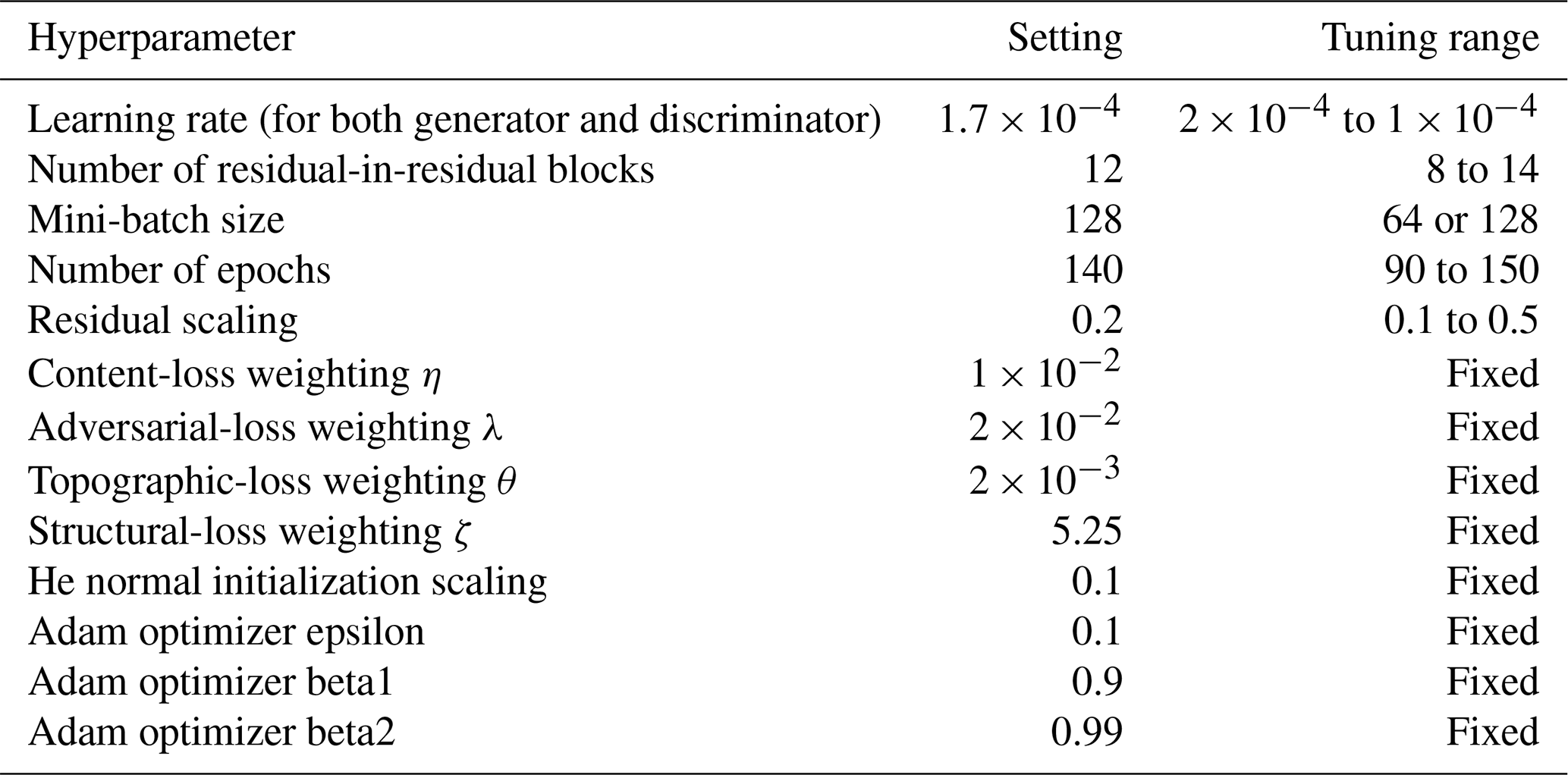
where η, λ, θ and ζ are the scaled weights for the content L1, adversarial LD, topographic LT and structural losses LS, respectively (see Table B1 for values used). The loss functions LD and LG are minimized in an alternate 1:1 manner so as to solve the entire generative adversarial network's objective function defined in Eq. (4).
The neural networks were developed using Chainer v7.0.0 (Tokui et al., 2019) and trained using full-precision (floating point 32) arithmetic. Experiments were carried out on four graphical processing units (GPUs), specifically two Tesla P100 GPUs and two Tesla V100 GPUs. On the Tesla V100 GPU setup, one training run with about 150 epochs takes about 30 min. This is using a batch size of 128 on a total of 3826 training image tiles, with 202 tiles reserved for validation, i.e. a 95∕5 training/validation split. We next describe the method used to evaluate each DeepBedMap candidate model, as well as the high-level way in which we semi-automatically arrived at a good model via semi-automatic hyperparameter tuning.
To check for overfitting, we evaluate the generative adversarial network model using the validation dataset after each epoch using two performance metrics – a peak signal-to-noise ratio (PSNR) metric for the generator and an accuracy metric for the discriminator. Training stops when these validation performance metrics show little improvement, roughly at 140 epochs.
Next, we conduct a full evaluation on an independent test dataset, comparing the model's predicted grid output with actual ground-truth xyz points. Using the “grdtrack” function in Generic Mapping Tools v6.0 (Wessel et al., 2019), we obtain the grid elevation at each ground-truth point and use it to calculate the elevation error on a point-to-point basis. All of these elevation errors are then used to compute a root mean square error (RMSE) statistic over this independent test site. This RMSE value is used to judge the model's performance in relation to baseline bicubic interpolation and is also the metric minimized by a hyperparameter optimization algorithm which we will describe next.
Neural networks contain a lot of hyperparameter settings that need to be decided upon, and generative adversarial networks are particularly sensitive to different hyperparameter settings. To stabilize model training and obtain better performance, we tune the hyperparameters (see Table B1) using a Bayesian approach. Specifically, we employ the Tree-structured Parzen Estimator (Bergstra et al., 2011) from the Optuna v2.0.0 (Akiba et al., 2019) library with default settings as per the Hyperopt library (Bergstra et al., 2015). Given that we have four GPUs, we choose to parallelize the hyperparameter tuning experiments asynchronously between all four devices. The estimator first conducts 20 random experimental trials to scan the hyperparameter space, gradually narrowing down its range to a few candidate hyperparameters in subsequent experiments. We set each GPU to run a target of 60 experimental trials (i.e. a total of 240), though unpromising trials that have exploding or vanishing gradients are pruned prematurely using the Hyperband algorithm (Li et al., 2018) to save on time and computational resources. The top models from these experiments undergo further visual evaluation, and we continue to conduct further experiments until a suitable candidate model is found.
Python code for data preparation, neural network model training and visualization of model outputs is freely available at https://github.com/weiji14/deepbedmap (last access: 9 August 2020) and at https://doi.org/10.5281/zenodo.3752613 (Leong and Horgan, 2020). Neural network model training experiment runs are also recorded at https://www.comet.ml/weiji14/deepbedmap (last access: 9 August 2020).
The DeepBedMap_DEM is available from Zenodo at https://doi.org/10.5281/zenodo.3752613 (Leong and Horgan, 2020). The Pine Island Glacier dataset (Bingham et al., 2017) is available on request from Robert Bingham. The Carlson Inlet dataset (King, 2011) is available on request from Edward King. Bed elevation datasets from Wilkes Subglacial Basin (Ferraccioli et al., 2018) and Rutford Ice Stream (King et al., 2016) are available from the British Antarctic Survey's Polar Data Centre (https://ramadda.data.bas.ac.uk, last access: 14 January 2020). Other Antarctic bed elevation datasets are available from the Center for Remote Sensing of Ice Sheets (https://data.cresis.ku.edu/data/rds, last access: 15 August 2019) or from the National Snow and Ice Data Center (https://nsidc.org/data/IRMCR2/versions/1, last access: 15 August 2019). BEDMAP2 (Fretwell et al., 2013) and REMA (Howat et al., 2018) are available from the Polar Geospatial Center (http://data.pgc.umn.edu, last access: 30 August 2019). MEaSUREs Ice Velocity data (Mouginot et al., 2019b) are available from NSIDC (https://nsidc.org/data/nsidc-0754/versions/1, last access: 31 August 2019). Antarctic snow accumulation data (Arthern et al., 2006) are available from the British Antarctic Survey (https://secure.antarctica.ac.uk/data/bedmap2/resources/Arthern_accumulation, last access: 17 June 2019).
WJL was responsible for data curation, formal analysis, methodology, software, visualization and writing the original draft. HJH was responsible for funding acquisition and supervision. Both authors conceptualized the work and contributed to the reviewing and editing stages of the writing.
The authors declare that they have no conflict of interest.
We are grateful to Robert Bingham and Edward King for the Pine Island Glacier and Carlson Inlet data and to all the other researchers in the British Antarctic Survey and Operation IceBridge team for providing free access to the high-resolution bed elevation datasets around Antarctica. A special thanks to Ruzica Dadic for her help in reviewing draft versions of this paper. This research was funded by the Royal Society of New Zealand's Rutherford Discovery Fellowship (contract RDF-VUW1602), with additional support from the Erasmus+ programme and International Glaciological Society early-career travel award for presenting earlier versions of this work at the 2019 EGU General Assembly and IGS Symposium on Five Decades of Radioglaciology.
This research has been supported by the Royal Society of New Zealand (Rutherford Discovery Fellowship – contract no. RDF-VUW1602).
This paper was edited by Olivier Gagliardini and reviewed by Martin Siegert and one anonymous referee.
Aitken, A. R. A., Young, D. A., Ferraccioli, F., Betts, P. G., Greenbaum, J. S., Richter, T. G., Roberts, J. L., Blankenship, D. D., and Siegert, M. J.: The subglacial geology of Wilkes Land, East Antarctica, Geophys. Res. Lett., 41, 2390–2400, https://doi.org/10.1002/2014GL059405, 2014. a
Akiba, T., Sano, S., Yanase, T., Ohta, T., and Koyama, M.: Optuna: A Next-generation Hyperparameter Optimization Framework, in: Proceedings of the 25th ACM SIGKDD International Conference on Knowledge Discovery & Data Mining – KDD '19, ACM Press, Anchorage, AK, USA, https://doi.org/10.1145/3292500.3330701, 2623–2631, 4–8 August 2019. a
Arthern, R. J., Winebrenner, D. P., and Vaughan, D. G.: Antarctic snow accumulation mapped using polarization of 4.3-cm wavelength microwave emission, J. Geophys. Res., 111, D06107, https://doi.org/10.1029/2004JD005667, 2006. a, b, c, d
Bergstra, J., Bardenet, R., Bengio, Y., and Kégl, B.: Algorithms for Hyper-Parameter Optimization, in: Proceedings of the 24th International Conference on Neural Information Processing Systems, NIPS'11, Curran Associates Inc., Granada, Spain, 2546–2554, 2011. a
Bergstra, J., Komer, B., Eliasmith, C., Yamins, D., and Cox, D. D.: Hyperopt: A Python Library for Model Selection and Hyperparameter Optimization, Computational Science & Discovery, 8, 014008, https://doi.org/10.1088/1749-4699/8/1/014008, 2015. a
Bindschadler, R., Choi, H., Wichlacz, A., Bingham, R., Bohlander, J., Brunt, K., Corr, H., Drews, R., Fricker, H., Hall, M., Hindmarsh, R., Kohler, J., Padman, L., Rack, W., Rotschky, G., Urbini, S., Vornberger, P., and Young, N.: Getting around Antarctica: new high-resolution mappings of the grounded and freely-floating boundaries of the Antarctic ice sheet created for the International Polar Year, The Cryosphere, 5, 569–588, https://doi.org/10.5194/tc-5-569-2011, 2011. a
Bingham, R. G., Vaughan, D. G., King, E. C., Davies, D., Cornford, S. L., Smith, A. M., Arthern, R. J., Brisbourne, A. M., De Rydt, J., Graham, A. G. C., Spagnolo, M., Marsh, O. J., and Shean, D. E.: Diverse landscapes beneath Pine Island Glacier influence ice flow, Nat. Commun., 8, 1618, https://doi.org/10.1038/s41467-017-01597-y, 2017. a, b, c, d
Blau, Y., Mechrez, R., Timofte, R., Michaeli, T., and Zelnik-Manor, L.: 2018 PIRM Challenge on Perceptual Image Super-resolution, arXiv:1809.07517 [cs], 2018. a
Chen, Z., Wang, X., Xu, Z., and Hou, W.: Convolutional Neural Network Based Dem Super Resolution, ISPRS – International Archives of the Photogrammetry, Remote Sensing and Spatial Information Sciences, XLI-B3, 247–250, https://doi.org/10.5194/isprsarchives-XLI-B3-247-2016, 2016. a
Clarke, G. K. C., Berthier, E., Schoof, C. G., and Jarosch, A. H.: Neural Networks Applied to Estimating Subglacial Topography and Glacier Volume, J. Climate, 22, 2146–2160, https://doi.org/10.1175/2008JCLI2572.1, 2009. a
Cornford, S. L., Martin, D. F., Lee, V., Payne, A. J., and Ng, E. G.: Adaptive Mesh Refinement versus Subgrid Friction Interpolation in Simulations of Antarctic Ice Dynamics, Ann. Glaciol., 57, 1–9, https://doi.org/10.1017/aog.2016.13, 2016. a
Cox, S. C., Smith-Lyttle, B., Siddoway, C., Capponi, G., Elvevold, S., Burton-Johnson, A., Halpin, J., Morin, P., Elliot, D., and Geomap Action Group: The GeoMAP dataset of Antarctic rock exposures, in: POLAR2018, p. 2428, Davos, Switzerland, 19–23 June 2018. a, b
Dai, J., Qi, H., Xiong, Y., Li, Y., Zhang, G., Hu, H., and Wei, Y.: Deformable Convolutional Networks, arXiv:1703.06211 [cs], 2017. a
Dong, C., Loy, C. C., He, K., and Tang, X.: Image Super-Resolution Using Deep Convolutional Networks, arXiv:1501.00092 [cs], 2014. a
Dowdeswell, J. A., Canals, M., Jakobsson, M., Todd, B. J., Dowdeswell, E. K., and Hogan, K. A.: The Variety and Distribution of Submarine Glacial Landforms and Implications for Ice-Sheet Reconstruction, Geol. Soc. Mem., 46, 519–552, https://doi.org/10.1144/M46.183, 2016a. a
Dowdeswell, J. A., Solheim, A., and Ottesen, D.: Rhombohedral Crevasse-Fill Ridges at the Marine Margin of a Surging Svalbard Ice Cap, Geol. Soc. Mem., 46, 73–74, https://doi.org/10.1144/M46.62, 2016b. a
Drews, R., Pattyn, F., Hewitt, I. J., Ng, F. S. L., Berger, S., Matsuoka, K., Helm, V., Bergeot, N., Favier, L., and Neckel, N.: Actively evolving subglacial conduits and eskers initiate ice shelf channels at an Antarctic grounding line, Nat. Commun., 8, 15228, https://doi.org/10.1038/ncomms15228, 2017. a
Dumoulin, V., Perez, E., Schucher, N., Strub, F., Vries, H., Courville, A., and Bengio, Y.: Feature-wise transformations, Distill, 3, e11, https://doi.org/10.23915/distill.00011, 2018. a, b
Durand, G., Gagliardini, O., Favier, L., Zwinger, T., and le Meur, E.: Impact of Bedrock Description on Modeling Ice Sheet Dynamics: Bedrock Description to Model Ice Sheet, Geophys. Res. Lett., 38, https://doi.org/10.1029/2011GL048892, 2011. a
Falcini, F. A., Rippin, D. M., Krabbendam, M., and Selby, K. A.: Quantifying Bed Roughness beneath Contemporary and Palaeo-Ice Streams, J. Glaciol., 64, 822–834, https://doi.org/10.1017/jog.2018.71, 2018. a
Farinotti, D., Huss, M., Bauder, A., Funk, M., and Truffer, M.: A Method to Estimate the Ice Volume and Ice-Thickness Distribution of Alpine Glaciers, J. Glaciol., 55, 422–430, https://doi.org/10.3189/002214309788816759, 2009. a
Farinotti, D., Brinkerhoff, D. J., Clarke, G. K. C., F”urst, J. J., Frey, H., Gantayat, P., Gillet-Chaulet, F., Girard, C., Huss, M., Leclercq, P. W., Linsbauer, A., Machguth, H., Martin, C., Maussion, F., Morlighem, M., Mosbeux, C., Pandit, A., Portmann, A., Rabatel, A., Ramsankaran, R., Reerink, T. J., Sanchez, O., Stentoft, P. A., Singh Kumari, S., van Pelt, W. J. J., Anderson, B., Benham, T., Binder, D., Dowdeswell, J. A., Fischer, A., Helfricht, K., Kutuzov, S., Lavrentiev, I., McNabb, R., Gudmundsson, G. H., Li, H., and Andreassen, L. M.: How accurate are estimates of glacier ice thickness? Results from ITMIX, the Ice Thickness Models Intercomparison eXperiment, The Cryosphere, 11, 949–970, https://doi.org/10.5194/tc-11-949-2017, 2017. a
Farinotti, D., Huss, M., Fürst, J. J., Landmann, J., Machguth, H., Maussion, F., and Pandit, A.: A Consensus Estimate for the Ice Thickness Distribution of All Glaciers on Earth, Nat. Geosci., 12, 168–173, https://doi.org/10.1038/s41561-019-0300-3, 2019. a
Ferraccioli, F., Corr, H., Jordan, T. A., Robinson, C., Armadillo, E., Bozzo, E., and Caneva, G.: Airborne radar bed elevation picks across the Wilkes Subglacial Basin, 2005–2006, Polar Data Centre, Natural Environment Research Council, UK, https://doi.org/10.5285/59e5a6f5-e67d-4a05-99af-30f656569401, 3 April 2018. a
Fretwell, P., Pritchard, H. D., Vaughan, D. G., Bamber, J. L., Barrand, N. E., Bell, R., Bianchi, C., Bingham, R. G., Blankenship, D. D., Casassa, G., Catania, G., Callens, D., Conway, H., Cook, A. J., Corr, H. F. J., Damaske, D., Damm, V., Ferraccioli, F., Forsberg, R., Fujita, S., Gim, Y., Gogineni, P., Griggs, J. A., Hindmarsh, R. C. A., Holmlund, P., Holt, J. W., Jacobel, R. W., Jenkins, A., Jokat, W., Jordan, T., King, E. C., Kohler, J., Krabill, W., Riger-Kusk, M., Langley, K. A., Leitchenkov, G., Leuschen, C., Luyendyk, B. P., Matsuoka, K., Mouginot, J., Nitsche, F. O., Nogi, Y., Nost, O. A., Popov, S. V., Rignot, E., Rippin, D. M., Rivera, A., Roberts, J., Ross, N., Siegert, M. J., Smith, A. M., Steinhage, D., Studinger, M., Sun, B., Tinto, B. K., Welch, B. C., Wilson, D., Young, D. A., Xiangbin, C., and Zirizzotti, A.: Bedmap2: improved ice bed, surface and thickness datasets for Antarctica, The Cryosphere, 7, 375–393, https://doi.org/10.5194/tc-7-375-2013, 2013. a, b, c, d, e, f, g, h, i, j, k, l
Fukushima, K. and Miyake, S.: Neocognitron: A New Algorithm for Pattern Recognition Tolerant of Deformations and Shifts in Position, Pattern Recogn., 15, 455–469, https://doi.org/10.1016/0031-3203(82)90024-3, 1982. a
GEBCO Bathymetric Compilation Group: The GEBCO_2020 Grid – a continuous terrain model of the global oceans and land. British Oceanographic Data Centre, National Oceanography Centre, NERC, UK, https://doi.org/10.5285/a29c5465-b138-234d-e053-6c86abc040b9, 2020. a
Glasser, N. F. and Gudmundsson, G. H.: Longitudinal surface structures (flowstripes) on Antarctic glaciers, The Cryosphere, 6, 383–391, https://doi.org/10.5194/tc-6-383-2012, 2012. a
Goff, J. A., Powell, E. M., Young, D. A., and Blankenship, D. D.: Conditional Simulation of Thwaites Glacier (Antarctica) Bed Topography for Flow Models: Incorporating Inhomogeneous Statistics and Channelized Morphology, J. Glaciol., 60, 635–646, https://doi.org/10.3189/2014JoG13J200, 2014. a
Goodfellow, I. J., Pouget-Abadie, J., Mirza, M., Xu, B., Warde-Farley, D., Ozair, S., Courville, A., and Bengio, Y.: Generative Adversarial Networks, arXiv:1406.2661 [cs, stat], 2014. a, b, c, d
Graham, F. S., Roberts, J. L., Galton-Fenzi, B. K., Young, D., Blankenship, D., and Siegert, M. J.: A high-resolution synthetic bed elevation grid of the Antarctic continent, Earth Syst. Sci. Data, 9, 267–279, https://doi.org/10.5194/essd-9-267-2017, 2017. a, b
Hättestrand, C.: Ribbed Moraines in Sweden – Distribution Pattern and Palaeoglaciological Implications, Sediment. Geol., 111, 41–56, https://doi.org/10.1016/S0037-0738(97)00005-5, 1997. a
Hättestrand, C. and Kleman, J.: Ribbed Moraine Formation, Quaternary Sci. Rev., 18, 43–61, https://doi.org/10.1016/S0277-3791(97)00094-2, 1999. a
He, K., Zhang, X., Ren, S., and Sun, J.: Deep Residual Learning for Image Recognition, arXiv:1512.03385 [cs], 2015. a
He, K., Zhang, X., Ren, S., and Sun, J.: Identity Mappings in Deep Residual Networks, arXiv:1603.05027 [cs], 2016. a
Helm, V., Humbert, A., and Miller, H.: Elevation and elevation change of Greenland and Antarctica derived from CryoSat-2, The Cryosphere, 8, 1539–1559, https://doi.org/10.5194/tc-8-1539-2014, 2014. a
Holschuh, N., Christianson, K., Paden, J., Alley, R. B., and Anandakrishnan, S.: Linking postglacial landscapes to glacier dynamics using swath radar at Thwaites Glacier, Antarctica, Geology, 48, 268–272, https://doi.org/10.1130/G46772.1, 2020. a, b
Howat, I. M., Paul, M., Claire, P., and Myong-Jong, N.: The Reference Elevation Model of Antarctica, Harvard Dataverse, https://doi.org/10.7910/DVN/SAIK8B, 2018. a, b
Howat, I. M., Porter, C., Smith, B. E., Noh, M.-J., and Morin, P.: The Reference Elevation Model of Antarctica, The Cryosphere, 13, 665–674, https://doi.org/10.5194/tc-13-665-2019, 2019. a, b, c, d
IMBIE: Mass Balance of the Antarctic Ice Sheet from 1992 to 2017, Nature, 558, 219–222, https://doi.org/10.1038/s41586-018-0179-y, 2018. a
Ioffe, S. and Szegedy, C.: Batch Normalization: Accelerating Deep Network Training by Reducing Internal Covariate Shift, arXiv:1502.03167 [cs], 2015. a
Isola, P., Zhu, J.-Y., Zhou, T., and Efros, A. A.: Image-to-Image Translation with Conditional Adversarial Networks, arXiv:1611.07004 [cs], 2016. a
Jeofry, H., Ross, N., Corr, H. F. J., Li, J., Gogineni, P., and Siegert, M. J.: 1-km bed topography digital elevation model (DEM) of the Weddell Sea sector, West Antarctica, https://doi.org/10.5281/zenodo.1035488, 2017. a
Jolicoeur-Martineau, A.: The Relativistic Discriminator: A Key Element Missing from Standard GAN, arXiv:1807.00734 [cs, stat], 2018. a
Jordan, T. A., Ferraccioli, F., Corr, H., Graham, A., Armadillo, E., and Bozzo, E.: Hypothesis for Mega-Outburst Flooding from a Palaeo-Subglacial Lake beneath the East Antarctic Ice Sheet: Antarctic Palaeo-Outburst Floods and Subglacial Lake, Terra Nova, 22, 283–289, https://doi.org/10.1111/j.1365-3121.2010.00944.x, 2010. a
Joughin, I., Tulaczyk, S., Bamber, J. L., Blankenship, D., Holt, J. W., Scambos, T., and Vaughan, D. G.: Basal Conditions for Pine Island and Thwaites Glaciers, West Antarctica, Determined Using Satellite and Airborne Data, J. Glaciol., 55, 245–257, https://doi.org/10.3189/002214309788608705, 2009. a
Kern, M., Cullen, R., Berruti, B., Bouffard, J., Casal, T., Drinkwater, M. R., Gabriele, A., Lecuyot, A., Ludwig, M., Midthassel, R., Navas Traver, I., Parrinello, T., Ressler, G., Andersson, E., Martin-Puig, C., Andersen, O., Bartsch, A., Farrell, S., Fleury, S., Gascoin, S., Guillot, A., Humbert, A., Rinne, E., Shepherd, A., van den Broeke, M. R., and Yackel, J.: The Copernicus Polar Ice and Snow Topography Altimeter (CRISTAL) high-priority candidate mission, The Cryosphere, 14, 2235–2251, https://doi.org/10.5194/tc-14-2235-2020, 2020. a
King, E. C.: Ice stream or not? Radio-echo sounding of Carlson Inlet, West Antarctica, The Cryosphere, 5, 907–916, https://doi.org/10.5194/tc-5-907-2011, 2011. a, b
King, E. C., Pritchard, H. D., and Smith, A. M.: Subglacial landforms beneath Rutford Ice Stream, Antarctica: detailed bed topography from ice-penetrating radar, Earth Syst. Sci. Data, 8, 151–158, https://doi.org/10.5194/essd-8-151-2016, 2016. a, b
Krizhevsky, A., Sutskever, I., and Hinton, G. E.: ImageNet Classification with Deep Convolutional Neural Networks, in: Advances in Neural Information Processing Systems 25, edited by: Pereira, F., Burges, C. J. C., Bottou, L., and Weinberger, K. Q., Curran Associates, Inc., Lake Tahoe, Nevada, 1097–1105, 2012. a
Kyrke-Smith, T. M., Gudmundsson, G. H., and Farrell, P. E.: Relevance of Detail in Basal Topography for Basal Slipperiness Inversions: A Case Study on Pine Island Glacier, Antarctica, Front. Earth Sci., 6, 33, https://doi.org/10.3389/feart.2018.00033, 2018. a
Le Brocq, A. M., Payne, A. J., and Vieli, A.: An improved Antarctic dataset for high resolution numerical ice sheet models (ALBMAP v1), Earth Syst. Sci. Data, 2, 247–260, https://doi.org/10.5194/essd-2-247-2010, 2010. a
LeCun, Y., Boser, B., Denker, J. S., Henderson, D., Howard, R. E., Hubbard, W., and Jackel, L. D.: Backpropagation Applied to Handwritten Zip Code Recognition, Neural Comput., 1, 541–551, https://doi.org/10.1162/neco.1989.1.4.541, 1989. a
Lecun, Y., Bottou, L., Bengio, Y., and Haffner, P.: Gradient-Based Learning Applied to Document Recognition, P. IEEE, 86, 2278–2324, https://doi.org/10.1109/5.726791, 1998. a
LeCun, Y., Bengio, Y., and Hinton, G.: Deep Learning, Nature, 521, 436–444, https://doi.org/10.1038/nature14539, 2015. a, b, c
Ledig, C., Theis, L., Huszar, F., Caballero, J., Cunningham, A., Acosta, A., Aitken, A., Tejani, A., Totz, J., Wang, Z., and Shi, W.: Photo-Realistic Single Image Super-Resolution Using a Generative Adversarial Network, in: 2017 IEEE Conference on Computer Vision and Pattern Recognition (CVPR), IEEE, Honolulu, Hawaii, 105–114, https://doi.org/10.1109/CVPR.2017.19, 21–26 July 2017. a
Leong, W. J. and Horgan, H. J.: DeepBedMap (Version v1.0.0), Zenodo, https://doi.org/10.5281/zenodo.3752614, 2020. a, b
Li, L., Jamieson, K., DeSalvo, G., Rostamizadeh, A., and Talwalkar, A.: Hyperband: A Novel Bandit-Based Approach to Hyperparameter Optimization, arXiv:1603.06560 [cs, stat], 2018. a
Lim, B., Son, S., Kim, H., Nah, S., and Lee, K. M.: Enhanced Deep Residual Networks for Single Image Super-Resolution, arXiv:1707.02921 [cs], 2017. a
Liu, X., Wang, Y., and Liu, Q.: PSGAN: A Generative Adversarial Network for Remote Sensing Image Pan-Sharpening, arXiv:1805.03371 [cs], 2018. a
Lythe, M. B. and Vaughan, D. G.: BEDMAP: A New Ice Thickness and Subglacial Topographic Model of Antarctica, J. Geophys. Res.-Sol. Ea., 106, 11335–11351, https://doi.org/10.1029/2000JB900449, 2001. a
Maas, A. L., Hannun, A. Y., and Ng, A. Y.: Rectifier nonlinearities improve neural network acoustic models, in ICML Workshop on Deep Learning for Audio, Speech, and Language Processing, Atlanta, Georgia, USA, 16 June 2013. a, b
Markus, T., Neumann, T., Martino, A., Abdalati, W., Brunt, K., Csatho, B., Farrell, S., Fricker, H., Gardner, A., Harding, D., Jasinski, M., Kwok, R., Magruder, L., Lubin, D., Luthcke, S., Morison, J., Nelson, R., Neuenschwander, A., Palm, S., Popescu, S., Shum, C., Schutz, B. E., Smith, B., Yang, Y., and Zwally, J.: The Ice, Cloud, and Land Elevation Satellite-2 (ICESat-2): Science Requirements, Concept, and Implementation, Remote Sens. Environ., 190, 260–273, https://doi.org/10.1016/j.rse.2016.12.029, 2017. a
Masi, G., Cozzolino, D., Verdoliva, L., and Scarpa, G.: Pansharpening by Convolutional Neural Networks, Remote Sens.-Basel, 8, 594, https://doi.org/10.3390/rs8070594, 2016. a
Monnier, J. and Zhu, J.: Inference of the bed topography in poorly flew over ice-sheets areas from surface data and a reduced uncertainty flow model, HAL Archives Ouvertes, available at: https://hal.archives-ouvertes.fr/hal-01926620 (last access: 7 March 2019), 2018. a
Morlighem, M.: MEaSUREs BedMachine Antarctica, Version 1, Boulder, Colorado, USA. NASA National Snow and Ice Data Center Distributed Active Archive Center, https://doi.org/10.5067/C2GFER6PTOS4, 2019. a, b, c
Morlighem, M., Rignot, E., Seroussi, H., Larour, E., Ben Dhia, H., and Aubry, D.: A Mass Conservation Approach for Mapping Glacier Ice Thickness: BALANCE THICKNESS, Geophys. Res. Lett., 38, https://doi.org/10.1029/2011GL048659, 2011. a
Morlighem, M., Williams, C. N., Rignot, E., An, L., Arndt, J. E., Bamber, J. L., Catania, G., Chauché, N., Dowdeswell, J. A., Dorschel, B., Fenty, I., Hogan, K., Howat, I., Hubbard, A., Jakobsson, M., Jordan, T. M., Kjeldsen, K. K., Millan, R., Mayer, L., Mouginot, J., Noël, B. P. Y., O'Cofaigh, C., Palmer, S., Rysgaard, S., Seroussi, H., Siegert, M. J., Slabon, P., Straneo, F., van den Broeke, M. R., Weinrebe, W., Wood, M., and Zinglersen, K. B.: BedMachine v3: Complete Bed Topography and Ocean Bathymetry Mapping of Greenland From Multibeam Echo Sounding Combined With Mass Conservation, Geophys. Res. Lett., 44, 11051–11061, https://doi.org/10.1002/2017GL074954, 2017. a
Morlighem, M., Rignot, E., Binder, T., Blankenship, D., Drews, R., Eagles, G., Eisen, O., Ferraccioli, F., Forsberg, R., Fretwell, P., Goel, V., Greenbaum, J. S., Gudmundsson, H., Guo, J., Helm, V., Hofstede, C., Howat, I., Humbert, A., Jokat, W., Karlsson, N. B., Lee, W. S., Matsuoka, K., Millan, R., Mouginot, J., Paden, J., Pattyn, F., Roberts, J., Rosier, S., Ruppel, A., Seroussi, H., Smith, E. C., Steinhage, D., Sun, B., Broeke, M. R. van den, Ommen, T. D. van, Wessem, M., and van and Young, D. A.: Deep glacial troughs and stabilizing ridges unveiled beneath the margins of the Antarctic ice sheet, Nat. Geosci., 13, 132–137, https://doi.org/10.1038/s41561-019-0510-8, 2019. a, b, c, d, e
Mouginot, J., Scheuchl, B., and Rignot, E.: MEaSUREs Antarctic Boundaries for IPY 2007–2009 from Satellite Radar, Version 2. Boulder, Colorado, USA, NASA National Snow and Ice Data Center Distributed Active Archive Center, https://doi.org/10.5067/AXE4121732AD, 2017. a
Mouginot, J., Rignot, E., and Scheuchl, B.: Continent-Wide, Interferometric SAR Phase, Mapping of Antarctic Ice Velocity, Geophys. Res. Lett., 46, 9710–9718, https://doi.org/10.1029/2019GL083826, 2019a. a
Mouginot, J., Rignot, E., and Scheuchl, B.: MEaSUREs Phase-Based Antarctica Ice Velocity Map, Version 1. Boulder, Colorado, USA, NASA National Snow and Ice Data Center Distributed Active Archive Center, https://doi.org/10.5067/PZ3NJ5RXRH10, 2019b. a, b, c, d, e
Nasrollahi, K. and Moeslund, T. B.: Super-Resolution: A Comprehensive Survey, Mach. Vision Appl., 25, 1423–1468, https://doi.org/10.1007/s00138-014-0623-4, 2014. a
Nias, I. J., Cornford, S. L., and Payne, A. J.: Contrasting the Modelled Sensitivity of the Amundsen Sea Embayment Ice Streams, J. Glaciol., 62, 552–562, https://doi.org/10.1017/jog.2016.40, 2016. a
Park, T., Liu, M.-Y., Wang, T.-C., and Zhu, J.-Y.: Semantic Image Synthesis with Spatially-Adaptive Normalization, arXiv:1903.07291 [cs], 2019. a
Raymond, M. J. and Gudmundsson, G. H.: On the relationship between surface and basal properties on glaciers, ice sheets, and ice streams, J. Geophys. Res.-Sol. Ea., 110, B08411, https://doi.org/10.1029/2005JB003681, 2005. a
Rignot, E., Mouginot, J., and Scheuchl, B.: Antarctic Grounding Line Mapping from Differential Satellite Radar Interferometry: Grounding Line of Antarctica, Geophys. Res. Lett., 38, https://doi.org/10.1029/2011GL047109, 2011. a
Rippin, D., Bingham, R., Jordan, T., Wright, A., Ross, N., Corr, H., Ferraccioli, F., Le Brocq, A., Rose, K., and Siegert, M.: Basal Roughness of the Institute and Möller Ice Streams, West Antarctica: Process Determination and Landscape Interpretation, Geomorphology, 214, 139–147, https://doi.org/10.1016/j.geomorph.2014.01.021, 2014. a
Robin, G. D. Q., Swithinbank, C., and Smith, B.: Radio Echo Exploration of the Antarctic Ice Sheet, in: International Symposium on Antarctic Glaciological Exploration (ISAGE), edited by: Gow, A., Keeler, C., Langway, C., and Weeks, W., no. 86 in IASH Publication, International Association of Scientific Hydrology, Hanover, New Hampshire, USA, 97–115, 1970. a
Rumelhart, D. E., Hinton, G. E., and Williams, R. J.: Learning Representations by Back-Propagating Errors, Nature, 323, 533–536, https://doi.org/10.1038/323533a0, 1986. a
Scambos, T.: Snow Megadune, Springer New York, New York, NY, https://doi.org/10.1007/978-1-4614-9213-9_620-1, 1–3, 2014. a
Scarpa, G., Vitale, S., and Cozzolino, D.: Target-Adaptive CNN-Based Pansharpening, IEEE T. Geosci. Remote, 56, 5443–5457, https://doi.org/10.1109/TGRS.2018.2817393, 2018. a
Sergienko, O. V. and Hindmarsh, R. C. A.: Regular Patterns in Frictional Resistance of Ice-Stream Beds Seen by Surface Data Inversion, Science, 342, 1086–1089, https://doi.org/10.1126/science.1243903, 2013. a
Shi, L., Allen, C. T., Ledford, J. R., Rodriguez-Morales, F., Blake, W. A., Panzer, B. G., Prokopiack, S. C., Leuschen, C. J., and Gogineni, S.: Multichannel Coherent Radar Depth Sounder for NASA Operation Ice Bridge, in 2010 IEEE International Geoscience and Remote Sensing Symposium, pp. 1729–1732, IEEE, Honolulu, HI, USA, https://doi.org/10.1109/IGARSS.2010.5649518, 25–30 July 2010. a, b
Siegert, M. J., Taylor, J., Payne, A. J., and Hubbard, B.: Macro-Scale Bed Roughness of the Siple Coast Ice Streams in West Antarctica, Earth Surf. Proc. Land., 29, 1591–1596, https://doi.org/10.1002/esp.1100, 2004. a
Simonyan, K. and Zisserman, A.: Very Deep Convolutional Networks for Large-Scale Image Recognition, arXiv:1409.1556 [cs], 2014. a
Solheim, A. and Pfirman, S. L.: Sea-floor morphology outside a grounded, surging glacier; Bråsvellbreen, Svalbard, Mar. Geol., 65, 127–143, https://doi.org/10.1016/0025-3227(85)90050-7, 1985. a
Tokui, S., Yamazaki Vincent, H., Okuta, R., Akiba, T., Niitani, Y., Ogawa, T., Saito, S., Suzuki, S., Uenishi, K., and Vogel, B.: Chainer: A Deep Learning Framework for Accelerating the Research Cycle, in: Proceedings of the 25th ACM SIGKDD International Conference on Knowledge Discovery & Data Mining – KDD '19, ACM Press, Anchorage, AK, USA, 2002–2011, https://doi.org/10.1145/3292500.3330756, 4–8 August 2019. a
Tsai, R. and Huang, T. S.: Multiframe Image Restoration and Registration, in: Advance Computer Visual and Image Processing, vol. 1, edited by: Huang, T. S., JAI Press, Greenwich, CT, 317–339, 1984. a
van Pelt, W. J. J., Oerlemans, J., Reijmer, C. H., Pettersson, R., Pohjola, V. A., Isaksson, E., and Divine, D.: An iterative inverse method to estimate basal topography and initialize ice flow models, The Cryosphere, 7, 987–1006, https://doi.org/10.5194/tc-7-987-2013, 2013. a
Wang, X., Yu, K., Wu, S., Gu, J., Liu, Y., Dong, C., Qiao, Y., and Loy, C. C.: ESRGAN: Enhanced Super-Resolution Generative Adversarial Networks, in: Computer Vision – ECCV 2018 Workshops, vol. 11133, edited by: Leal-Taixé, L. and Roth, S., Springer International Publishing, Cham, https://doi.org/10.1007/978-3-030-11021-5_5, 63–79, 2019. a, b, c, d, e, f, g
Wang, Z., Bovik, A., Sheikh, H., and Simoncelli, E.: Image Quality Assessment: From Error Visibility to Structural Similarity, IEEE T. Image Process., 13, 600–612, https://doi.org/10.1109/TIP.2003.819861, 2004. a
Wessel, P., Luis, J., Uieda, L., Scharroo, R., Wobbe, F., Smith, W., and Tian, D.: The Generic Mapping Tools Version 6, Geochem. Geophy. Geosy., 20, 5556–5564, https://doi.org/10.1029/2019GC008515, 2019. a, b
Xu, Z., Wang, X., Chen, Z., Xiong, D., Ding, M., and Hou, W.: Nonlocal Similarity Based DEM Super Resolution, ISPRS J. Photogramm., 110, 48–54, https://doi.org/10.1016/j.isprsjprs.2015.10.009, 2015. a
Yang, J., Fu, X., Hu, Y., Huang, Y., Ding, X., and Paisley, J.: PanNet: A Deep Network Architecture for Pan-Sharpening, in: 2017 IEEE International Conference on Computer Vision (ICCV), IEEE, Venice, Italy, 1753–1761, https://doi.org/10.1109/ICCV.2017.193, 22–29 October 2017. a
Yang, W., Zhang, X., Tian, Y., Wang, W., Xue, J.-H., and Liao, Q.: Deep Learning for Single Image Super-Resolution: A Brief Review, IEEE T. Multimedia, 21, 3106–3121, https://doi.org/10.1109/TMM.2019.2919431, 2019. a, b
- Abstract
- Introduction
- Related work
- Data and methods
- Results
- Discussion
- Conclusions
- Appendix A: Details of loss function components
- Appendix B: Neural network training details
- Code availability
- Data availability
- Author contributions
- Competing interests
- Acknowledgements
- Financial support
- Review statement
- References