the Creative Commons Attribution 4.0 License.
the Creative Commons Attribution 4.0 License.
 | 31 Oct 2020
Investigation of spatial and temporal variability of river ice phenology and thickness across Songhua River Basin, northeast China
Qian Yang
Kaishan Song
Xiaohua Hao
Zhidan Wen
Yue Tan
Weibang Li
The regional role and trends of freshwater ice are critical factors for aquatic ecosystems, climate variability, and human activities. The ice regime has been scarcely investigated in the Songhua River Basin of northeast China. Using daily ice records of 156 hydrological stations across the region, we examined the spatial variability in the river ice phenology and river ice thickness from 2010 to 2015 and explored the role of snow depth and air temperature on the ice thickness. The river ice phenology showed a latitudinal distribution and a changing direction from southeast to northwest. We identified two spatial clusters based on Moran's I spatial autocorrelation, and results showed that the completely frozen duration with high values clustered in the Xiao Hinggan Range and that with low values clustered in the Changbai Mountains at the 95 % confidence level. The maximum ice thickness over 125 cm was distributed along the ridge of the Da Hinggan Range and Changbai Mountains, and the maximum ice thickness occurred most often in February and March. In three subbasins of the Songhua River Basin, we developed six Bayesian regression models to predict ice thickness from air temperature and snow depth. The goodness of the fit (R2) for these regression models ranged from 0.80 to 0.95, and the root mean square errors ranged from 0.08 to 0.18 m. Results showed significant and positive correlations between snow cover and ice thickness when freshwater was completely frozen. Ice thickness was influenced by the cumulative air temperature of freezing through the heat loss of ice formation and decay instead of just air temperature.
- Article
(7113 KB) - Full-text XML
- BibTeX
- EndNote


The freeze–thaw process of temperate lakes' and rivers' surface ice plays a crucial role in the interactions among the climate system (Yang et al., 2020), the freshwater ecosystem (Kwok and Fahnestock, 1996), and the biological environment (Prowse and Beltaos, 2002). The presence of freshwater ice is closely associated with social and economic activities, such as from human-made structures, water transportation, and winter recreation (Lindenschmidt et al., 2017; Williams and Stefan, 2006). Ice cover on rivers and lakes exerts large forces due to thermal expansion and could cause extensive infrastructure losses to bridges, docks, and shorelines (Shuter et al., 2012). Ice cover on waterbodies also provides a natural barrier between the atmosphere and the water. Moreover, ice cover also blocks the solar radiation which is necessary for photosynthesis to provide enough dissolved oxygen for fish, thus posing a negative effect on freshwater ecosystems. In extreme cases, it can lead to the winter deaths of fish (Hampton et al., 2017). Generally, the duration of freshwater ice has shown a declining trend with later freeze-up and earlier break-up throughout the Northern Hemisphere. For example, the freeze-up has been occurring 0.57 d later per decade and the break-up 0.63 d earlier per decade during the period of 1846–1995 (Beltaos and Prowse, 2009; Magnuson et al., 2000; Sharma et al., 2019). Despite the growing importance of river ice under global warming, very little work has been undertaken to explain the considerable variation of ice characteristics in northeast China, where lakes and rivers are frozen for as long as 5 to 6 months a year. A robust and quantitative investigation on the variations of the river ice regime associated with changes in snow depth on ice and air temperature are fundamental for understanding climate changes at regional scales.
The earliest ice record in the literature dates back to the 1840s in the Northern Hemisphere (Magnuson et al., 2000). Ice development and ice diversity scales have been regarded as sensitive climate indicators. Ice phenology and ice thickness have been studied to obtain a deeper understanding of ice processes. The optical remote sensing data at medium and large scales are widely adopted for deriving ice phenology (Šmejkalová et al., 2016; Song et al., 2014). In contrast, microwave remote sensing is used to estimate ice thickness and snow depth over ice (Kang et al., 2014; Zhang et al., 2019). Wide-ranging satellites make it possible to link ice characteristic with climate indices, such as air temperature (Yang et al., 2020) and large-scale teleconnections (Ionita et al., 2018). Still, their spatial resolutions are too coarse to detect ice thickness and the snow depth over ice at local scales accurately. For example, the microwave satellite data of the Advanced Microwave Scanning Radiometer for the Earth Observing System (AMSR-E) have a spatial resolution of 25 km, but the largest width of the Nenjiang River only ranges from 1700 to 1800 m. The spatial resolution limits the ability of satellite observations to inverse ice thickness precisely, let alone the snow depth.
In terms of point-based measurements, the most commonly used ground observations include the fixed-station observations, the ice charts, the volunteer monitoring, and the field measurements (Duguay et al., 2015). Ground observations depend on the spatial distribution and the representation, which are limited by the accessibility of surface-based networks. Various models, such as physically based models (Park et al., 2016), linear regressions (Palecki and Barry, 1986; Williams and Stefan, 2006), logistic regressions (Yang et al., 2020), and artificial neural networks (Seidou et al., 2006; Zaier et al., 2010), have been developed to derive ice phenology and ice thickness. The physically based models mainly consider the energy exchange and physical changes in freshwater ice and require detailed information and data support, including hydrological, meteorological, hydraulic, and morphological information (Rokaya et al., 2020). As the relevant information at local scales is more readily available, the physically based models are more suitable for small watershed applications (e.g., within 100 km2). On the other hand, empirical models are more commonly adopted to predict changes in the ice regime from relatively limited climate data available over larger basins (Yang et al., 2020). Ice parameters, such as ice thickness and freeze-up and break-up dates, differ notably from point to point on a given river continuum (Pavelsky and Smith, 2004), and the uneven distribution of hydrological stations poses an obstacle for spatial investigation and modeling. Therefore, sufficient historical ice records are necessary to model the ice regime and validate the reliability of remote sensing data.
The ice cover of water bodies experiences three stages: the freeze-up, the ice growth, and the break-up (Duguay et al., 2015). The ice phenology, the ice thickness, and the ice composition change considerably in different stages. Although air temperature influences the freeze–thaw cycle of river ice dramatically, the effect of snow cover cannot be ignored. Generally, the effect of snow depth on the ice forming process is more vital than the impact of air temperature (Morris et al., 2005; Park et al., 2016). In contrast to these studies, Stefan and Fang (1997) found that the air temperature had a more substantial effect on the ice thickness formation than the snow depth. Furthermore, in situ observations at Russian river mouths, where ice thickness has decreased, did not show any striking correlation between the ice thickness and the snow depth (Shiklomanov and Lammers, 2014). Previous studies have analyzed the relationship in view of spatial distributions but ignored the frozen status of ice formation processes. The relative influence of snow depth and air temperature on the freshwater ice regimes in northeast China calls for a detailed exploration.
To estimate the interaction between the ice regime and the climate systems, a comprehensive investigation and robust analysis of the ice regime are essential in providing relevant information for projecting future changes in the ice regime. The work is the first to present continuous river ice records of three sub-catchments of the Songhua River Basin from 2010 to 2015, and the study compares the spatial and temporal changes in ice phenology and ice thickness. The influence of snow cover and air temperature on the ice regime is quantitatively explored in the three sub-catchments in order to consider the frozen status of the river ice.
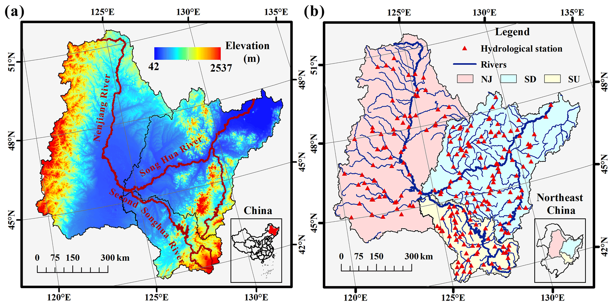
Figure 1The geographic location of the Songhua River Basin showing (a) the elevation and (b) the location of 156 hydrological stations. The Songhua River Basin includes three subbasins: the Nenjiang River Basin (NJ), the downstream Songhua River Basin (SD), and the upstream Songhua River Basin (SU). Elevation data are from the Shuttle Radar Topography Mission (SRTM) with a spatial resolution of 90 m.
2.1 Study area
The Songhua River Basin is located in the middle area of northeast China (Fig. 1), which includes Liaoning Province, Jilin Province, Heilongjiang Province, and the eastern part of the Inner Mongolia Autonomous Region. The Songhua River is the third-longest river in China and has three main tributaries, namely, the Nenjiang River, the main Songhua River, and the second Songhua River (Khan et al., 2018; Zhao et al., 2018). The basins of the three tributary rivers include the Nenjiang River Basin (NJ), the downstream Songhua River Basin (SD), and the upstream Songhua River Basin (SU) (Fig. 1). The Nenjiang River is 1370 km in length, and the corresponding drainage has an area of 2.55×10⁶ km2. The main Songhua River has a length of 939 km, and the downstream catchment of the Songhua River Basin (SD) covers an area of 1.86×10⁶ km2. The second Songhua River has a length of 958 km, and the upstream catchment of the Songhua River Basin has an area of 6.19×10⁵ km2 (Chen et al., 2019; Yang et al., 2018). Temperate and cold temperate climates characterize the whole Songhua River Basin; winter is long and cold, and spring is windy and dry. The annual average air temperature ranges between 3 and 5∘C, while yearly precipitation ranges from 400 to 800 mm from the southeast to the northwest region (Wang et al., 2015, 2018).
2.2 Data source
2.2.1 Ice phenology
The ice records were obtained from the annual hydrological report, including ice phenology, yearly maximum ice thickness of the river center, and the corresponding day of year (DOY) (Hydrographic bureau of Chinese Ministry of Water Resources, 2010–2015). There were 50, 35, and 71 hydrological stations in the NJ, SU, and SD basins, totalling 156 stations. Five lake ice phenologies were available, and the definitions are listed below (Duguay et al., 2015; Hydrographic bureau of Chinese Ministry of Water Resources, 2015).
-
The freeze-up start is considered the first day when the floating ice can be observed with temperatures below 0∘C.
-
The freeze-up end is the day when a steady ice carapace can be observed on the river and the area of ice cover takes up more than 80 % in the view range.
-
The break-up start is the first day when ice melting can be observed with surface ponding.
-
The break-up end is the day when the surface is mainly covered by open water and the area of open water exceeds 20 %.
-
The complete frozen duration regards the ice cover duration when the lake is completely frozen during the winter period from freeze-up end to break-up start.
2.2.2 Ice thickness
We used ice thickness, snow depth, and air temperature from 120 stations for the period ranging from 2010 to 2015 to study changes in ice thickness and establish the regression model described below. There were 37, 28, and 55 stations located in the NJ, SU, and SD basins, respectively. The hydrological report also provided ice thickness, snow depth on ice, and air temperature on bank every 5 d from November through April, totalling 37 measurements in one cold season. The average snow depths were derived from the mean of three or four measurements around the ice hole for ice thickness measurements without human disturbances (Hydrographic bureau of Chinese Ministry of Water Resources, 2015). To enhance the performance of the regression model, the cumulative air temperature of freezing was derived from air temperature from November to March.
2.3 Data analysis
Our overall method can be summarized in the following steps. First, we used kriging to spatially interpolate in situ measurements of ice phenology. Second, we used Moran's I spatial autocorrelation to identify spatial clusters based on the interpolated ice phenology data. Finally, we analyzed the drivers of spatial and temporal variability of the river ice thickness for each cluster. To do so, we used Bayesian linear regression to quantify the links between the river ice thickness and snow depth and air temperature.
2.3.1 Kriging
Kriging has been widely applied to spatially interpolate in situ measurements of ice phenology (Choinski et al., 2015; Jenson et al., 2007), such as freeze-up start, freeze-up end, break-up start, break-up end, and complete frozen duration. The average values of five ice phenologies were calculated during the period from 2010 to 2015 and explored accordingly with the Geostatistical Analyst software of ArcGIS. The interpolation results exhibited their spatial distribution. We chose the ordinary kriging method and set the variation function as the spherical model. Moreover, isophanes connecting locations with the same ice phenology were also graphed with the interpolation results (Paramasivam and Venkatramanan, 2019).
2.3.2 Moran's I
Moran's I, developed by Patrick Alfred Pierce Moran, aims to observe the spatial autocorrelation, and the spatial autocorrelation is characterized by a correlation in a signal among nearby locations in space (Li et al., 2020). We calculated the Global Moran's I and Anselin Local Moran's I of the complete frozen duration and ice thickness in the ArcGIS software environment. The Moran's I indicates whether the distribution of regional values is aggregated, discrete, or random (Mitchell, 2005). A positive Moran's I indicates a tendency toward clustering, while a negative Moran's I indicates a tendency of dispersion (Castro and Singer, 2006). The Anselin Local Moran's I statistics identified the clustered spots, and those which were statistically significant were evaluated by the combined thresholds of the z score or p values.
2.3.3 Bayesian linear regression
Ice thickness had been modeled by the air temperature and the snow depth using Bayesian linear regression, which has been widely adopted in hydrological and environmental analysis (Gao et al., 2014; Zhao et al., 2013). Bayesian linear regression views regression coefficients and the disturbance variance as random variables rather than fixed and unknown quantities. This assumption leads to a more flexible model and intuitive inferences (Barber, 2008). The Bayesian linear regression model was implemented in two models: a prior probability model considered the probability distribution of the regression coefficients and the disturbance, and a posterior model predicted the response using the prior probability mentioned below. Using k fold cross-validation, we divided the input dataset into five equal subsets or folds and used four subsets as the training set and the remaining as the testing set. The performance of the regression model was evaluated with the determination coefficient (R2) and the root mean square error (RMSE).
In this paper, we treated ice thickness on the river as the Y data and snow depth over ice and air temperature as the X data with a dataset size of 31. The ice thickness was measured on the river every 5 d from November to March when the river was completely covered with ice with air temperature below 0∘C. Air temperature and cumulative air temperature of freezing were considered in modeling. Additionally, the Pearson correlation was calculated to analyze the relationship between the five ice phenology events and ice-related parameters, including maximum ice thickness, snow depth on ice, and air temperature on bank.
3.1 Spatial variations of river ice phenology
The river ice phenology was analyzed herein, including freeze-up start, freeze-up end, break-up start, break-up end, and complete frozen duration. The hydrological report only supplied one record of river ice phenology each year for all the 156 stations. For each hydrological station, the average values of five river ice phenologies were calculated from the ice records from 2010 to 2015 and interpolated by the kriging method to analyze the spatial distribution of the river ice phenology.
3.1.1 Freeze-up end and break-up process
Figure 2 illustrates the average spatial distribution of the freeze-up start, the freeze-up end, and the isophanes in the Songhua River Basin of northeast China from 2010 to 2015. Figure 3 shows the spatial distribution of the break-up start and the break-up end. The corresponding statistics are listed in Table 1. Freeze-up start ranged from 28 October to 21 November with a mean value of 7 November, and freeze-up end ranged from 7 November to 8 December with a mean value of 22 November. Break-up start ranged from 24 March to 20 April with a mean value of 9 April, and break-up end ranged from 31 March to 27 April with a mean value of 15 April. These four parameters showed a latitudinal gradient: freeze-up start and freeze-up end decreased, while break-up start and break-up end increased with the increase in latitude except in the NJ basin. The middle part of the NJ basin had the highest freeze-up start and freeze-up end and decreased to the southern and northern parts. As the latitude decreased, the air temperature tended to increase, leading to later freeze-up and earlier break-up times with shorter ice-covered durations, and vice versa.
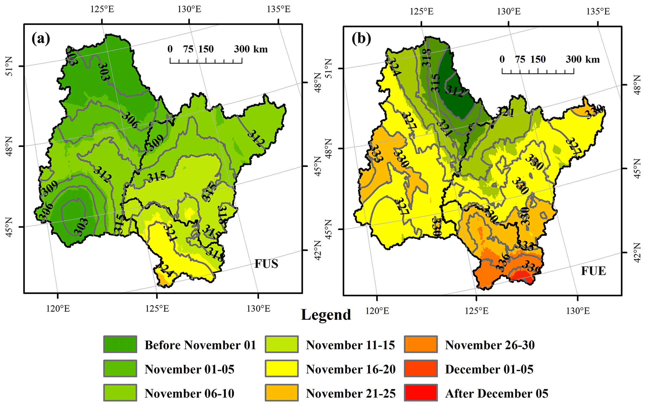
Figure 2The average spatial distribution of freeze-up start (FUS) (a) and freeze-up end (FUE) (b) in the Songhua River Basin of northeast China from 2010 to 2015. The number labels indicate the day of year (DOY) of the isophenes.
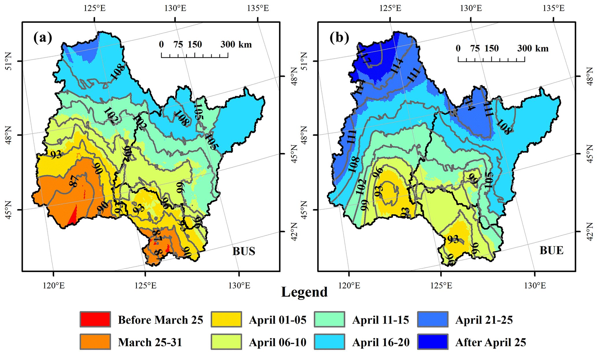
Figure 3The average spatial distribution of break-up start (BUS) (a) and break-up end (BUE) (b) in the Songhua River Basin of northeast China from 2010 to 2015. The number labels indicate the day of year (DOY) of the isophenes.
Table 1Summary of statistics of ice phenology interpolated by the kriging method from 2010 to 2015. The ice phenology indicators included freeze-up start (FUS), freeze-up end, break-up start (BUS), break-up end (BUE), and complete frozen duration (CFD). NJ, SD, and SU represent the Nenjiang Basin, the downstream Songhua River Basin, and the upstream Songhua River Basin. DOY denotes day of year. Std. dev. denotes standard deviation.
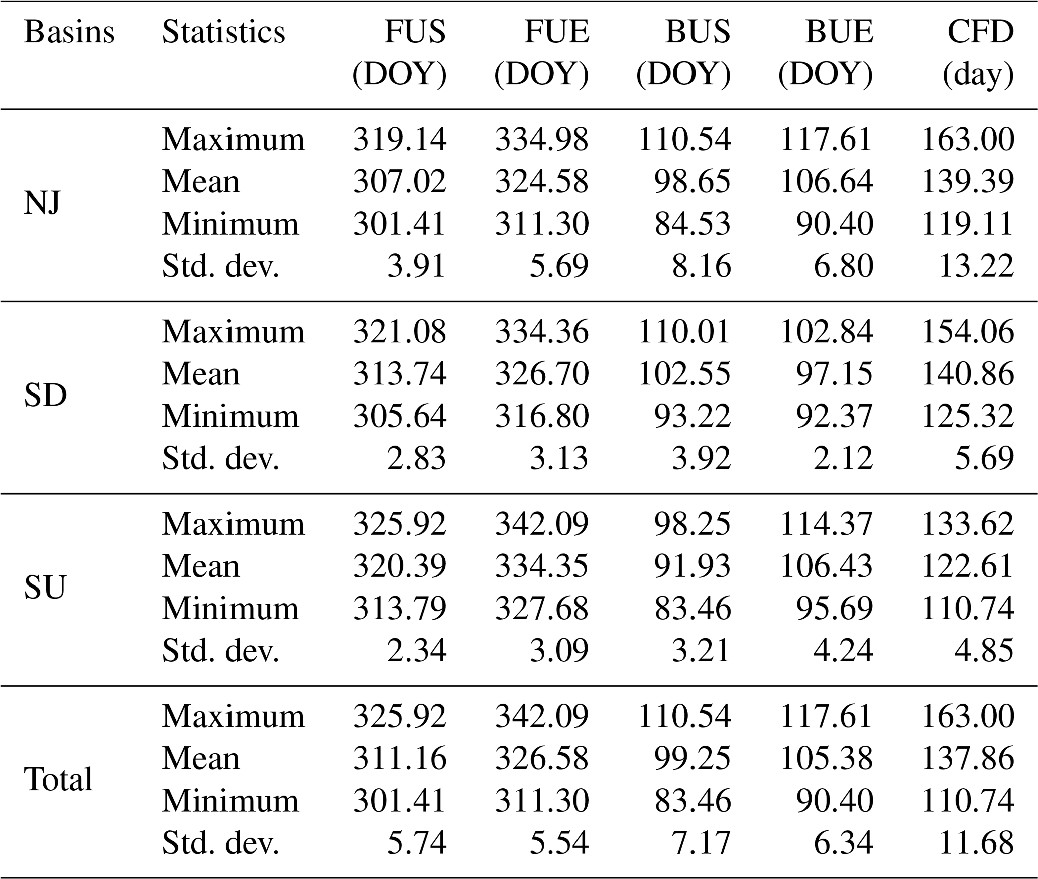
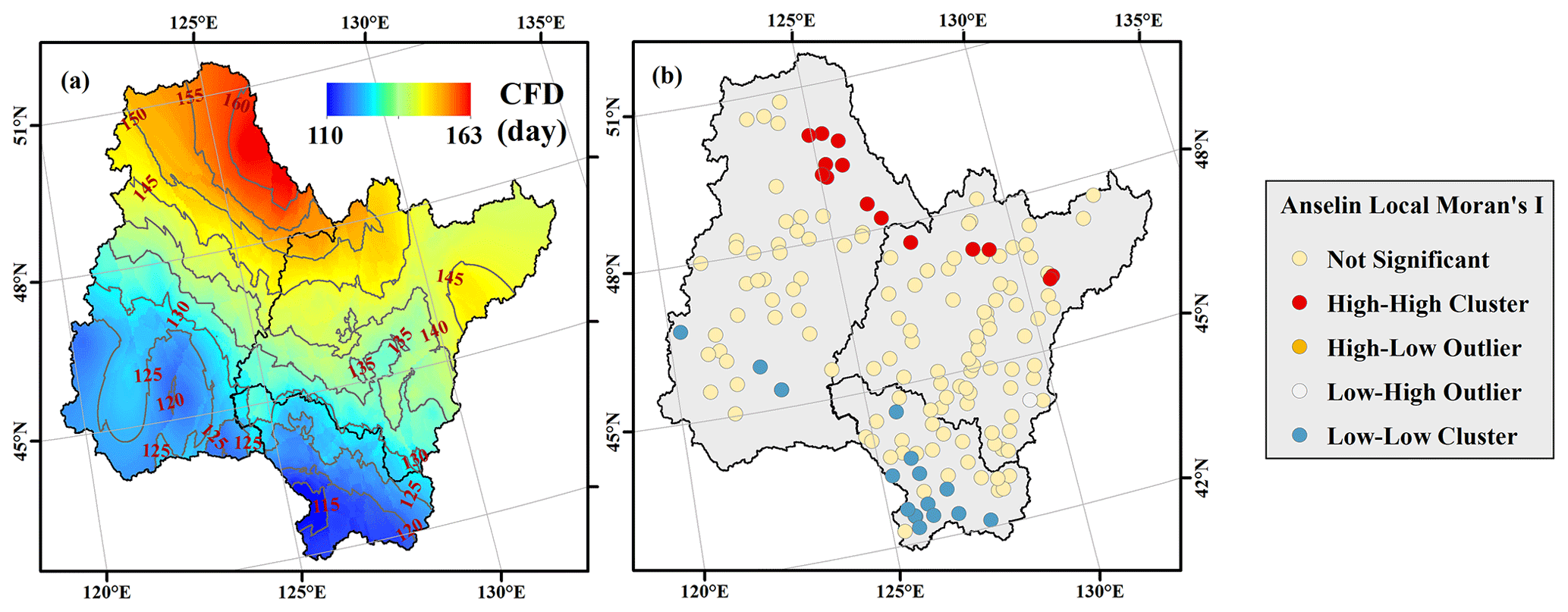
Figure 4The spatial distribution of complete frozen duration (a) interpolated using the kriging method and Anselin Local Moran's I (b) in the Songhua River Basin of northeast China.
3.1.2 Complete frozen duration
Figure 4a illustrates the average spatial distribution of complete frozen duration interpolated by kriging and the isophanes in the Songhua River Basin from 2010 to 2015. The complete frozen duration ranged from 110.74 to 163.00 d with a mean value of 137.86 d which increased with latitude. Interestingly, the isophanes of complete frozen duration had different directionality, increasing from the southeast to northwest, which could also be found in the other parameters. Both freeze-up start and freeze-up end correlated negatively with the latitude with coefficients of −0.66 and −0.53, respectively (n=156, p<0.001). However, the break-up start, the break-up end, and the complete frozen duration were all positively correlated with latitude with coefficients of 0.48, 0.57, and 0.55, respectively (n=156, p<0.001). We built the linear regression equations between the river ice phenology and latitude. As the latitude increased by 1∘C, freeze-up start and freeze-up end occurred 2.56 and 2.32 d early, and the break-up start and break-up end arrived 2.36 and 2.37 d late, causing an increase of 4.68 d for the complete frozen duration. This could be explained by the decreasing solar radiation with latitude influencing the ice thaw and melting processes directly.
The Global Moran's I statistics of the complete frozen duration were 1.36 with a z score and p value of 2.41 and 0.02, which indicates that the complete frozen duration exhibited a clustered pattern with a confidence level of 95 % for the whole basin. Then Anselin Local Moran's I was calculated to identify statistically significant spatial outliers for each hydrological location in Fig. 4c. Results showed that 14 of 156 hydrological stations showed a statistically significant cluster of high values, 17 of 156 showed a statistically significant cluster of low values, and 125 of 156 showed no significant cluster at the 95 % confidence level. Both Global and Local Moran's I results indicated that the high values of complete frozen duration clustered along the Xiao Hinggan Range and that the low values of complete frozen duration grouped around the Changbai Mountains.
3.2 Variations of ice thickness
We explored the spatial pattern of ice thickness using the yearly maximum ice thickness gathered from 156 stations and examined the seasonal changes in ice thickness, snow depth on ice, and air temperature based on the time series from November to April.

Figure 5The spatial distribution of yearly maximum ice thickness (MIT) of the river center (a) and the corresponding date (b).
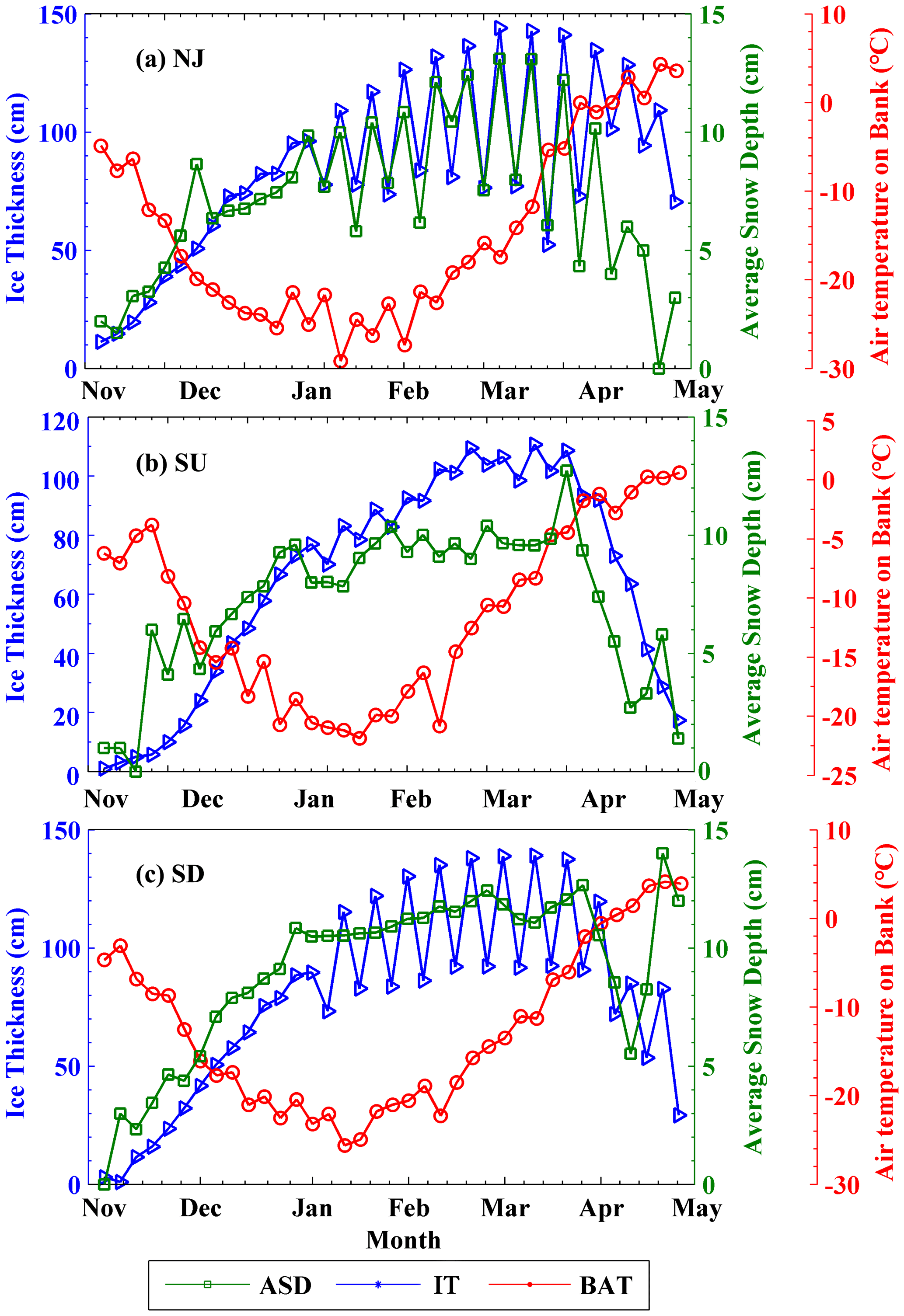
Figure 6Average seasonal changes in ice thickness (IT), average snow depth (ASD), and air temperature on bank (BAT) from November to April for the period 2010–2015.
3.2.1 Spatial patterns of ice thickness
Figure 5 illustrates the spatial distribution of the yearly maximum ice thickness of the river center and the corresponding DOY. Table 2 summarizes the statistical results of maximum ice thickness and the DOY. Maximum ice thickness ranged from 12 cm to 146 m with an average value of 78 cm. The maximum ice thickness between 76 and 100 cm accounted for the most significant percentage of 43.33 %, followed by 31.67 % for maximum ice thickness between 50 and 75 cm. As shown in Table 2, five stations had a more exceptional maximum ice thickness than 125 cm. The DOY of maximum ice thickness had an average value of 21 February, and maximum ice thickness mainly occurred 59 and 40 times in February and March, respectively. Four of the five highest maximum ice thicknesses greater than 125 cm happened in March, which is consistent with the interannual changes in ice development shown in Fig. 6. The results suggest that the river ice was always the thickest and the steadiest in February or March, which has important implications for human activities, such as ice fishing and entertainment. The ice thickness did not show the same latitudinal distribution as ice phenology, which suggests that more climate factors should be taken into consideration, such as snow depth and wind speed.
Table 2The frequency of yearly maximum ice thickness from November to April. The first column represents different months in the cold season, and the other columns represent yearly maximum ice thickness (MIT) with the unit in centimeters.
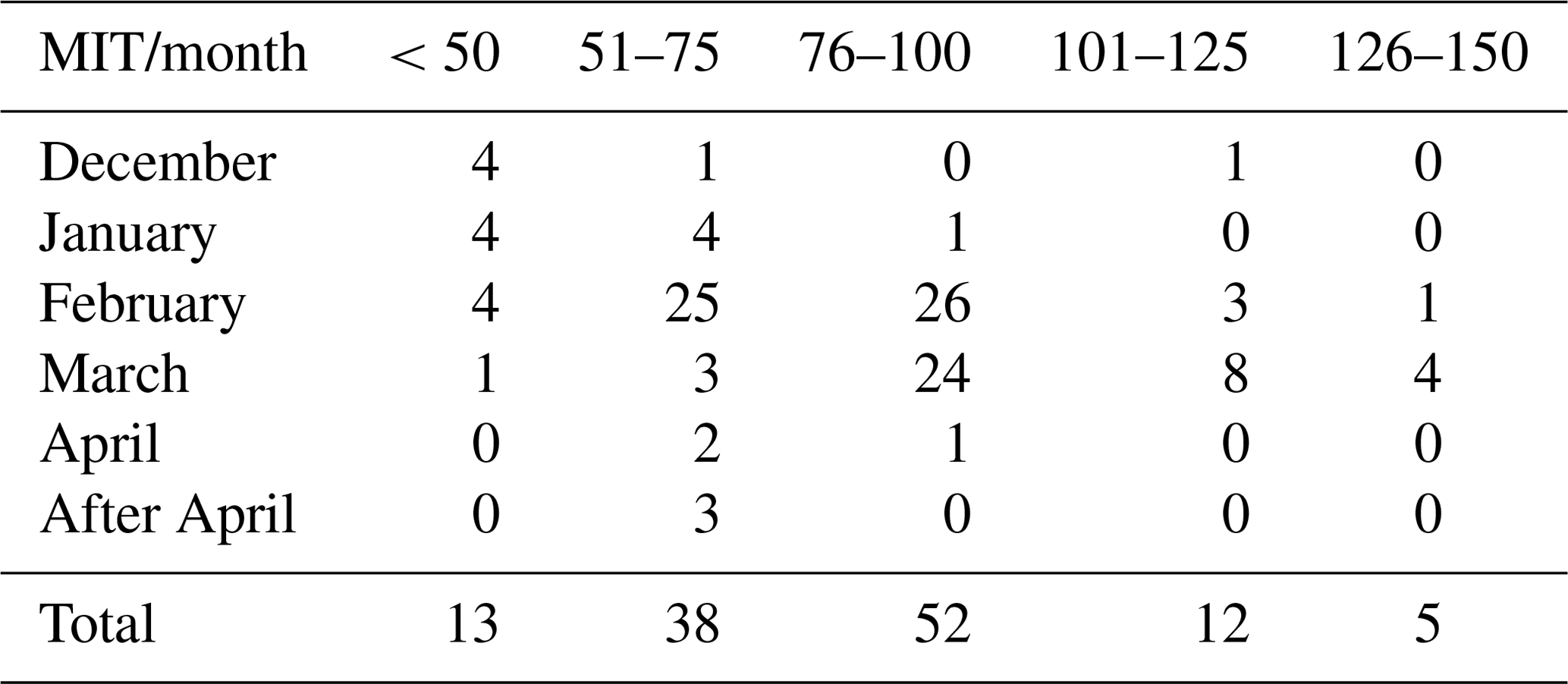
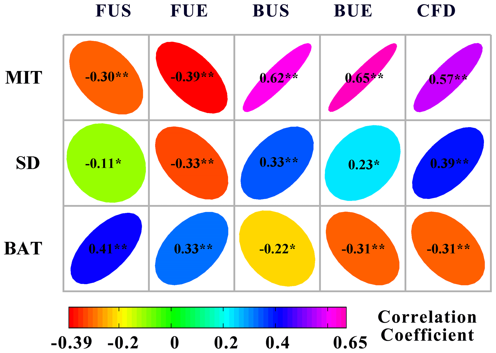
Figure 7Correlation matrix between maximum ice thickness (MIT), snow depth (SD), and air temperature on bank (BAT) and lake ice phenology events with data from 120 stations. The asterisks indicate the significance level of the correlation coefficients: means significant at 99 % level (p<0.01), and * means significant at 95 % level (p<0.05).
3.2.2 Seasonal changes in ice thickness
Figure 6 displays the seasonal changes in ice development using ice thickness, average snow depth on ice, and air temperature, which was collected on the bank every 5 d from November to April during the period between 2010 and 2015. The variations of ice characteristics differed significantly due to time and location. Among the three basins, the NJ basin had the lowest air temperature of ∘C, followed by ∘C in the SD basin and ∘C in the SU basin. The SD basin had the highest snow depth of 9.18 ± 3.39 cm on the average level, followed by 8.35 ± 4.60 cm in the SU basin and 8.23 ± 3.92 cm in the NJ basin. The changes in daily ice thickness and snow depth had a similar overall trend, while air temperature followed the opposite pattern. Both ice thickness and snow depth increased from November, reached a peak in March, and then dropped at the beginning of April. The air temperature showed a distinct trend and reached the lowest in the middle of February, which is earlier than the peaks of maximum ice thickness and snow depth. In Fig. 6, the day when ice thickness reached the maximum value was 50, 54, and 60 d later than the day when air temperature reached the lowest value in the NJ, SU, and SD basin, respectively.
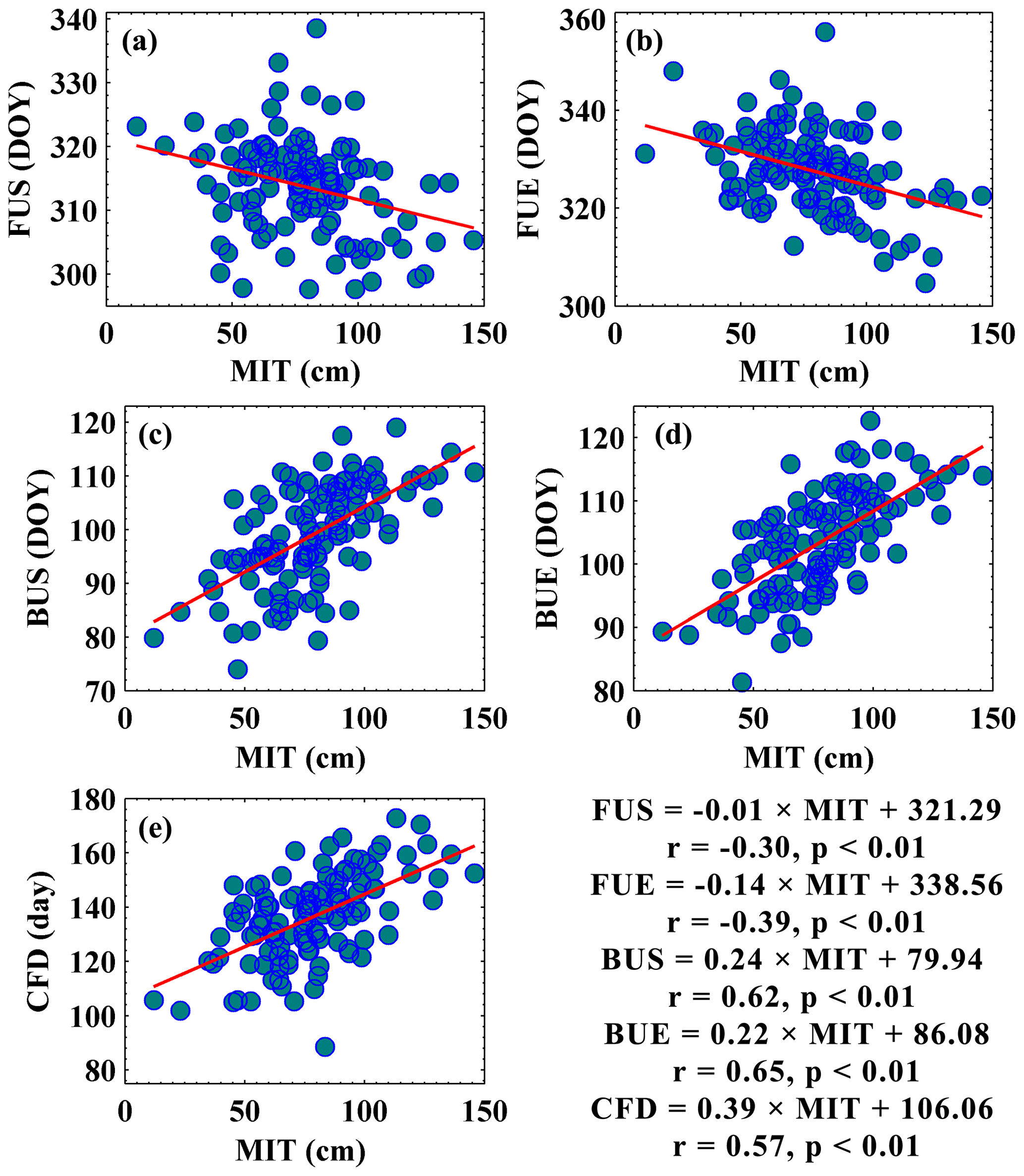
Figure 8The bivariate scatter plots with linear regression lines between yearly maximum ice thickness (MIT) and ice phenology with a dataset size of 120; r and p denote the correlation coefficient and p value of the regression line. The ice phenology events include freeze-up start (FUS), freeze-up end (FUE), break-up start (BUS), break-up end (BUE), and complete frozen duration (CFD).
3.3 The relationship between ice regime and climate factors
3.3.1 Correlation analysis
Figure 7 displays the correlation matrix between lake ice phenology events and three ground measurements from 120 hydrological stations. The lake ice phenology events included the freeze-up start, the freeze-up end, the break-up start, the break-up end, and the complete frozen duration. The three ground measurements covered the yearly mean values of snow depth, the air temperature on bank, and the maximum ice thickness. The color intensity and sizes of the ellipses are proportional to the correlation coefficients. The maximum ice thickness had a higher correlation with four of the five indices than snow depth and air temperature on bank except with freeze-up start. The maximum ice thickness and break-up end had the highest correlation of 0.63 (n=120, p<0.01). During the freeze-up process, two freeze-up dates had a negative association with the maximum ice thickness and snow depth. During the break-up process, two break-up dates had positive correlations with maximum ice thickness and snow depth. The complete frozen duration showed a positive correlation with the maximum ice thickness and the snow depth and a negative correlation with air temperature. Regarding the annual changes, no significant correlation was found between snow depth and five ice phenology events in Fig. 7.
Figure 8 shows the bivariate scatter plots between the yearly maximum ice thickness and the ice phenology along with regression equations attached. The break-up process had a negative correlation with the maximum ice thickness, while the freeze-up had a positive correlation. Moreover, the break-up process had a higher correlation with the maximum ice thickness, and the break-up end had the highest correlation coefficients with the maximum ice thickness of 0.65 (p<0.01). The complete frozen duration also had a positive correlation with a maximum ice thickness of 0.57 (p<0.01), which means that a thicker ice cover in winter can lead to a delay in the melting time in spring. The break-up does not only depend on the spring climate conditions, but it is also influenced by the ice thickness during the preceding winter. A thicker ice cover stores more heat in winter, taking a longer time to melt in spring (Yang et al., 2019). The limited performance of the regression model can be attributed to the difficulties in determining river ice phenology. Although a uniform specification for ice regime observations was required, the inhomogeneities among different stations could not be ignored.
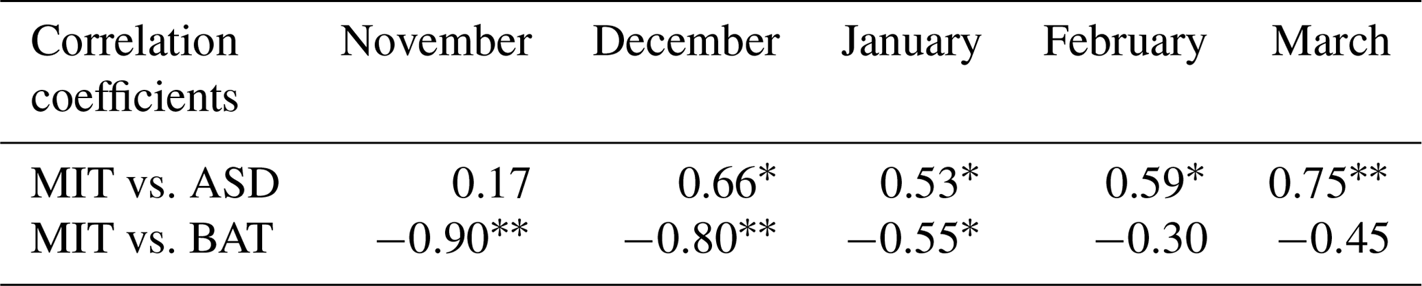
To further explore the role of snow cover, the monthly correlation coefficients between the ice thickness, the snow depth, and the air temperature on bank were calculated and are listed in Table 3. The correlation coefficients between the ice thickness and the snow depth increased from November to March and reached a peak of 0.75 in March when ice was the thickest. This indicated an increasingly important role of the snow depth on the ice thickness as the ice accumulated. The higher correlation coefficients between the ice thickness and the air temperature on bank in November and December revealed that the air temperature played a more critical role in the freeze-up process. The positive correlation coefficient between snow depth and ice thickness (Table 3) showed two opposite effects of the snow depth during ice development. During the ice-growth process, snow depth protects the ice from cold air and slows down the growth rate of ice thickness. During the ice-decay process, the lake bottom ice stops growing, the surface snow or ice melts, and slush forms accordingly. The melting speed depends on the ability to absorb heat, and the slush can absorb more heat, which would promote melting (Kirillin et al., 2012). The slush often exists in multiple freeze–thaw cycles of river ice before it completely disappears. Therefore, when studying the role of snow cover, the status of river ice can not be neglected.
Table 3Correlation coefficients between maximum ice thickness (MIT) and average snow depth (ASD) and air temperature on bank (BAT) with a dataset size of 120 stations. The asterisks indicate the significant level of correlation coefficients: means significant at 99 % level (p<0.01), and * means significant at 95 % level (p<0.05).
3.3.2 Regression modeling
We carried out a cross-validation for Bayesian linear regression using the k fold method, and the K value was set as 5. For each iteration, a different fold was used for testing, and the remaining four subsets were applied for training. The training and testing were repeated for five iterations. Table 4 lists the R2 of the training and testing process for each iteration. The best Bayesian linear regression was determined when the bias between testing and training regressions was the smallest. The corresponding R2 of the best regression is shown in bold in Table 4.
Table 4The cross-validation of Bayesian linear regression using the k fold method, and the K value was set as 5. Ice thickness was treated as dependent variables, and air temperature and snow depth on ice were treated as independent variables. Air temperature and cumulative air temperature of freezing were considered in the model building. The R2 values of the best linear regression avoiding over-fitting are marked in bold.

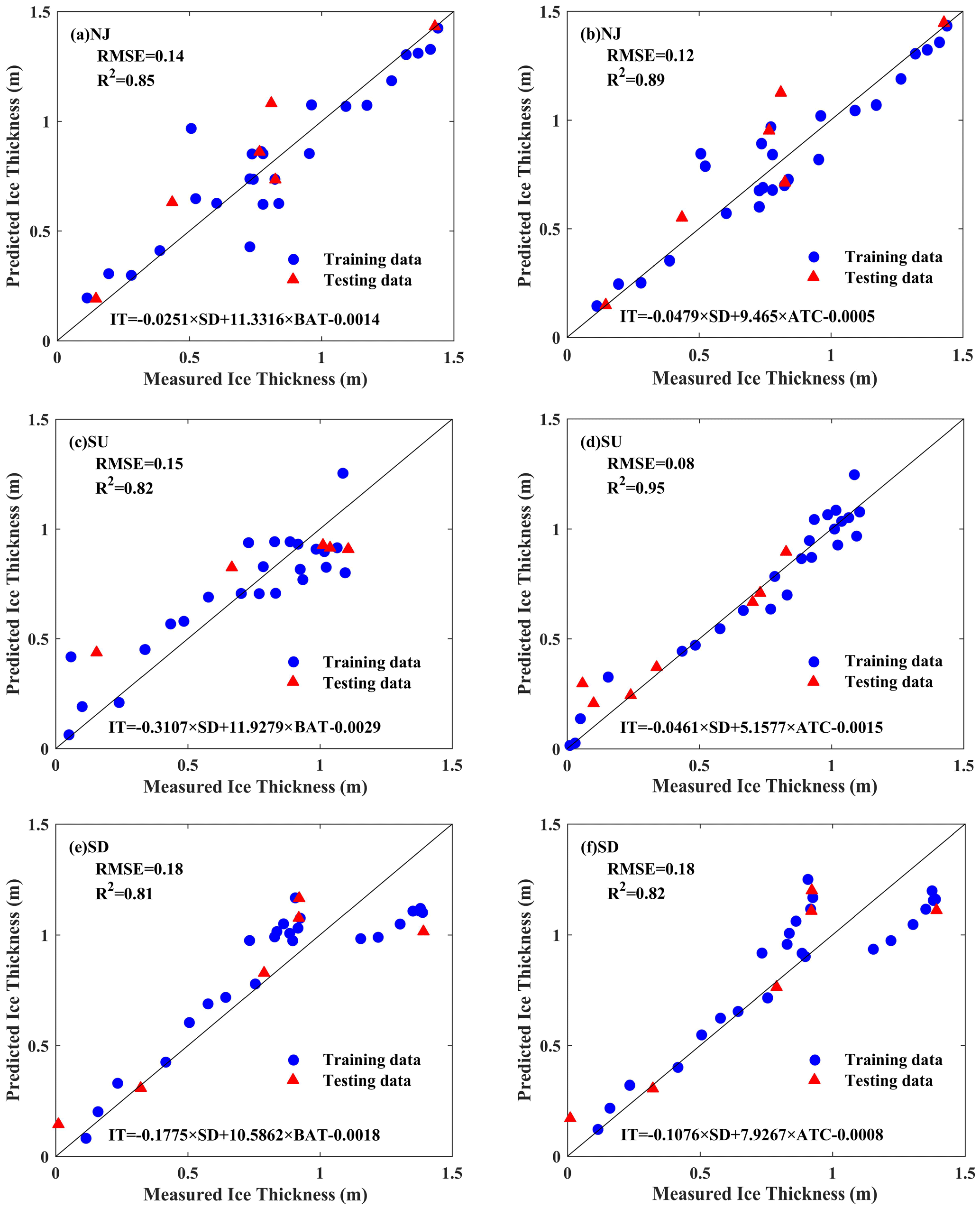
Figure 9Scatter plots between measured and predicted ice thicknesses using Bayesian linear regression in three subbasins (NJ: Nenjiang Basin; SU: upstream Songhua River Basin; and SD: downstream Songhua River Basin) in northeast China. The model treated ice thickness as the independent variable and snow depth and air temperature as dependent variables. Two types of air temperature were used: BAT represents air temperature on bank, and ATC represents the cumulative air temperature of freezing.
Figure 9 illustrates the scatter plot between the measured and the predicted ice thickness with Bayesian linear regression in three subbasins in northeast China. From Fig. 9, the R2 of Bayesian linear regression varies from 0.81 to 0.95, and RMSE varies from 0.08 to 0.18 m. The model works best in the SU basin, followed by the NJ and the SD basins. Figure 9 indicates that the snow depth outweighs the air temperature in terms of the effect on ice thickness, which is consistent with previous studies (Magnuson et al., 2000; Sharma et al., 2019). Moreover, replacing air temperature on bank with cumulative air temperature of freezing enhanced the model performance in all three basins, revealing a more important role of cumulative air temperature of freezing than air temperature. For the Bayesian linear regressions, we used the field measurements that spanned from November to March, thus focusing only on the coldest part of the year. During this period, the river surface is completely frozen, and the air temperature that falls below 0∘C promotes the ice growth. April is the month when the rise in air temperatures above 0∘C enables the river ice to melt.
The correlation between air temperature and ice regime in Fig. 7 was not as significant as was found in some previous studies (Park et al., 2016; Stefan and Fang, 1997). One of the reasons is that previous studies often averaged the air temperatures over a longer period and at a regional scale, therefore losing the signal on seasonality at a local scale (Pavelsky and Smith, 2004; Yang et al., 2020). To circumvent this shortcoming, we applied the regression analysis on seasonal time series of ice thickness and air temperature. Our work considered this and established the regression using the seasonal time series of ice thickness and air temperature. When building the Bayesian regression equation, the increasing R2 showed that the cumulative air temperature of freezing behaved better than the air temperature on bank, which suggests that heat exchanges between river surface and atmosphere dominate the ice process. Heat loss is mainly made up of sensible and latent heat exchange (Beltaos and Prowse, 2009; Robertson et al., 1992) , which is proportional to the cumulative air temperature of freezing during the cooling process. During the complete frozen duration, the snow depth, along with the wind speed, began to influence the heat exchange and ice thickening. Air temperature exerted a lesser vital effect on spring break-up, which is more dependent on the ice thickness and the snow depth. In summary, snow depth dominated the ice process when the river was completely frozen. At the same time, the cumulative air temperature was dominant during the transition process between open water and completely frozen conditions.
Five river ice phenology proxies, including freeze-up end, freeze-up start, break-up end, break-up start, and complete frozen duration in the Songhua River Basin of northeast China, have been investigated using in situ measurements for the period from 2010 to 2015. According to the spatial distribution interpolated by the ordinary kriging method, the river ice phenology indicators followed the latitudinal gradient and a changing direction from southeast to northwest. As the latitude increased by 1∘C, the freeze-up start and freeze-up end happened 2.56 and 2.32 d earlier, and the break-up start and break-up end arrived 2.36 and 2.37 d later, resulting in a 4.68 d increase in complete frozen duration.
The spatial autocorrelation of the completely frozen duration and maximum ice thickness has been explored by Global and Anselin Local Moran's I. The Global Moran's I with a z score of 1.36 showed that the complete frozen duration exhibited a clustered pattern at the 95 % confidence level. In contrast, the maximum ice thickness did not show a significantly clustered pattern. The Anselin Local Moran's I results indicated that the high values of complete frozen duration clustered along the Xiao Hinggan Range and that the low values of the complete frozen duration clustered in the Changbai Mountains. The maximum ice thickness over 125 cm was distributed along the ridge of the Da Hinggan Range and Changbai Mountains, and maximum ice thickness occurred most often in February and March during the cold season.
Based on the analysis of monthly time series measurements, snow cover played an increasingly important role as the river became completely frozen. The temporal variability in air temperature was more correlated with the variability in ice phenology, while snow depth was more correlated with ice thickness. Six Bayesian regression models were established for the ice thickness, air temperature, and snow depth in three subbasins of the Songhua River with respect to air temperature and cumulative air temperature. Results showed that snow cover correlated with ice thickness significantly and positively during the periods when the freshwater was completely frozen. In line with the performance metrics (R2, root mean square error), the cumulative air temperature of freezing was shown to provide a better predictor than the air temperature in simulating the ice thickness changes compared to the air temperature.
This study provides a quantitative investigation of the ice regime in the Songhua River Basin of northeast China and established potential regression models for projecting future changes in the ice regime. Remote sensing data could provide long-term and wide-ranging information on ice thickness and ice phenology from 1980 onwards. Data analyzed in this study present a valuable reference for future studies that rely on remote sensing observations of the river ice thickness in this area. Therefore, we plan to use satellite data to enlarge our study scope in our future work.
The data that support the findings of this study are available from the corresponding author upon reasonable request.
KS and QY designed the idea of this study together. QY and ZW wrote the paper and analyzed the data cooperatively. XH provided valuable suggestions for the structure of the study and paper. WL and YT exerted efforts on data processing and graphing. This article is a result of a collaboration between all listed coauthors.
The authors declare that they have no conflict of interest.
The anonymous reviewers who improved the quality of this paper are much appreciated.
This research has been supported by the National Natural Science Foundation of China (grant nos. 41801283, 41971325, and 41730104).
This paper was edited by Valentina Radic and reviewed by two anonymous referees.
Barber, J. J.: Bayesian Core: A Practical Approach to Computational Bayesian Statistics, J. Am. Stat. Assoc., 103, 432–433, 2008.
Beltaos, S. and Prowse, T.: River-ice hydrology in a shrinking cryosphere, Hydrol. Process., 23, 122–144, https://doi.org/10.1002/hyp.7165, 2009.
Castro, M. C. D. and Singer, B. H.: Controlling the False Discovery Rate: A New Application to Account for Multiple and Dependent Tests in Local Statistics of Spatial Association, Geogr. Anal., 38, 180–208, 2006.
Chen, H., Zhang, W., Nie, N., and Guo, Y.: Long-term groundwater storage variations estimated in the Songhua River Basin by using GRACE products, land surface models, and in-situ observations, Sci. Total Environ., 649, 372–387, 2019.
Choinski, A., Ptak, M., Skowron, R., and Strzelczak, A.: Changes in ice phenology on polish lakes from 1961 to 2010 related to location and morphometry, Limnologica, 53, 42–49, 2015.
Duguay, C. R., Bernier, M., Gauthier, Y., and Kouraev, A.: Remote sensing of lake and river ice, in: Remote Sensing of the Cryosphere, edited by: Tedesco, M., John Wiley & Sons, Ltd, Hoboken, New Jersey, USA, 273–306, https://doi.org/10.1002/9781118368909.ch12, 2015.
Gao, S., Zhu, Z., Liu, S., Jin, R., Yang, G., and Tan, L.: Estimating the spatial distribution of soil moisture based on Bayesian maximum entropy method with auxiliary data from remote sensing, Int. J. Appl. Earth Obs., 32, 54–66, 2014.
Hampton, S. E., Galloway, A. W., Powers, S. M., Ozersky, T., Woo, K. H., Batt, R. D., Labou, S. G., O'Reilly, C. M., Sharma, S., Lottig, N. R., Stanley, E. H., North, R. L., Stockwell, J. D., Adrian, R., Weyhenmeyer, G. A., Arvola, L., Baulch, H. M., Bertani, I., Bowman Jr., L. L., Carey, C. C., Catalan, J., Colom-Montero, W., Domine, L. M., Felip, M., Granados, I., Gries, C., Grossart, H. P., Haberman, J., Haldna, M., Hayden, B., Higgins, S. N., Jolley, J. C., Kahilainen, K. K., Kaup, E., Kehoe, M. J., MacIntyre, S., Mackay, A. W., Mariash, H. L., McKay, R. M., Nixdorf, B., Noges, P., Noges, T., Palmer, M., Pierson, D. C., Post, D. M., Pruett, M. J., Rautio, M., Read, J. S., Roberts, S. L., Rucker, J., Sadro, S., Silow, E. A., Smith, D. E., Sterner, R. W., Swann, G. E., Timofeyev, M. A., Toro, M., Twiss, M. R., Vogt, R. J., Watson, S. B., Whiteford, E. J., and Xenopoulos, M. A.: Ecology under lake ice, Ecol. Lett., 20, 98–111, 2017.
Hydrographic bureau of Chinese Ministry of Water Resources: Annual hydrological report: hydrological data of Heilongjiang River Basin, China water resources and Hydropower Press, Beijing, China, 2010–2015.
Hydrographic bureau of Chinese Ministry of Water Resources: Specification for observation of ice regime in rivers, China water resources and Hydropower Press, Beijing, China, 2015.
Ionita, M., Badaluta, C. A., Scholz, P., and Chelcea, S.: Vanishing river ice cover in the lower part of the Danube basin – signs of a changing climate, Sci. Rep., 8, 7948, https://doi.org/10.1038/s41598-018-26357-w, 2018.
Jenson, B. J., Magnuson, J. J., Card, V. M., Soranno, P. A., and Stewart, K. M.: Spatial Analysis of Ice Phenology Trends across the Laurentian Great Lakes Region during a Recent Warming Period, Limnol. Oceanogr., 52, 2013–2026, 2007.
Kang, K. K., Duguay, C. R., Lemmetyinen, J., and Gel, Y.: Estimation of ice thickness on large northern lakes from AMSR-E brightness temperature measurements, Remote Sens. Environ., 150, 1–19, 2014.
Khan, M. I., Liu, D., Fu, Q., and Faiz, M. A.: Detecting the persistence of drying trends under changing climate conditions using four meteorological drought indices, Meteorol. Appl., 25, 184–194, 2018.
Kirillin, G., Lepparanta, M., Terzhevik, A., Granin, N., Bernhardt, J., Engelhardt, C., Efremova, T., Golosov, S., Palshin, N., Sherstyankin, P., Zdorovennova, G., and Zdorovennov, R.: Physics of seasonally ice-covered lakes: a review, Aquat. Sci., 74, 659–682, 2012.
Kwok, R. and Fahnestock, M. A.: Ice Sheet Motion and Topography from Radar Interferometry, IEEE T. Geosci. Remote, 34, 189–200, 1996.
Li, R., Chen, N., Zhang, X., Zeng, L., Wang, X., Tang, S., Li, D., and Niyogi, D.: Quantitative analysis of agricultural drought propagation process in the Yangtze River Basin by using cross wavelet analysis and spatial autocorrelation, Agr. Forest Meteorol., 280, 107809, https://doi.org/10.1016/j.agrformet.2019.107809, 2020.
Lindenschmidt, K.-E., Das, A., and Chu, T.: Air pockets and water lenses in the ice cover of the Slave River, Cold Reg. Sci. Technol., 136, 72–80, 2017.
Magnuson, J. J., Robertson, D. M., Benson, B. J., Wynne, R. H., Livingstone, D. M., Arai, T., Assel, R. A., Barry, R. G., Card, V., and Kuusisto, E.: Historical Trends in Lake and River Ice Cover in the Northern Hemisphere, Science, 289, 1743–1746, 2000.
Mitchell, A.: The ESRI Guide to GIS Analysis, VI, 238, ESRI Press, Redlands, California, available at: http://www.doc88.com/p-3897763072733.html (last access: 1 December 2017), 2005.
Morris, K., Jeffries, M., and Duguay, C.: Model simulation of the effects of climate variability and change on lake ice in central Alaska, USA, Ann. Glaciol., 40, 113–118, https://doi.org/10.3189/172756405781813663, 2005.
Palecki, M. A. and Barry, R. G.: Freeze-up and Break-up of Lakes as an Index of Temperature Changes during the Transition Seasons: A Case Study for Finland, J. Appl. Meteorol., 25, 893–902, 1986.
Paramasivam, C. R. and Venkatramanan, S.: An Introduction to Various Spatial Analysis Techniques, in: GIS and Geostatistical Techniques for Groundwater Science, edited by: Venkatramanan, S., Prasanna, M. V., and Chung, S. Y., Elsevier, Amsterdam, the Netherlands, 23–30, https://doi.org/10.1016/B978-0-12-815413-7.00003-1, 2019.
Park, H., Yoshikawa, Y., Oshima, K., Kim, Y., Ngo-Duc, T., Kimball, J. S., and Yang, D.: Quantification of Warming Climate-Induced Changes in Terrestrial Arctic River Ice Thickness and Phenology, J. Climate, 29, 1733–1754, 2016.
Pavelsky, T. M. and Smith, L. C.: Spatial and temporal patterns in Arctic river ice breakup observed with MODIS and AVHRR time series, Remote Sens. Environ., 93, 328–338, 2004.
Prowse, T. D. and Beltaos, S.: Climatic control of river-ice hydrology: a review, Hydrol. Process., 16, 805–822, https://doi.org/10.1002/hyp.369, 2002.
Robertson, D. M., Ragotzkie, R. A., and Magnuson, J. J.: Lake ice records used to detect historical and future climatic changes, Climatic Change, 21, 407–427, 1992.
Rokaya, P., Morales-Marin, L., and Lindenschmidt, K.-E.: A physically-based modelling framework for operational forecasting of river ice breakup, Adv. Water Resour., 139, 103554, https://doi.org/10.1016/j.advwatres.2020.103554, 2020.
Seidou, O., Ouarda, T. B. M. J., Bilodeau, L., Bruneau, B., and St-Hilaire, A.: Modeling ice growth on Canadian lakes using artificial neural networks, Water Resour. Res., 42, 2526–2528, 2006.
Sharma, S., Blagrave, K., Magnuson, J. J., O'Reilly, C. M., Oliver, S., Batt, R. D., Magee, M. R., Straile, D., Weyhenmeyer, G. A., Winslow, L., and Woolway, R. I.: Widespread loss of lake ice around the Northern Hemisphere in a warming world, Nat. Clim. Change, 9, 227–231, 2019.
Shiklomanov, A. I. and Lammers, R. B.: River ice responses to a warming Arctic – recent evidence from Russian rivers, Environ. Res. Lett., 9, 035008, https://doi.org/10.1088/1748-9326/9/3/035008, 2014.
Shuter, B. J., Finstad, A. G., Helland, I. P., Zweimüller, I., and Hölker, F.: The role of winter phenology in shaping the ecology of freshwater fish and their sensitivities to climate change, Aquat. Sci., 74, 637–657, 2012.
Šmejkalová, T., Edwards, M. E., and Dash, J.: Arctic lakes show strong decadal trend in earlier spring ice-out, Scient. Rep., 6, 38449, https://doi.org/10.1038/srep38449, 2016.
Song, C., Huang, B., Ke, L., and Richards, K. S.: Remote sensing of alpine lake water environment changes on the Tibetan Plateau and surroundings: A review, ISPRS J. Photogram. Remote Sens., 92, 26–37, 2014.
Stefan, H. G. and Fang, X.: Simulated climate change effects on ice and snow covers on lakes in a temperate region, Cold Reg. Sci. Technol., 25, 137–152, 1997.
Wang, M., Lei, X., Liao, W., and Shang, Y.: Analysis of changes in flood regime using a distributed hydrological model: a case study in the Second Songhua River basin, China, Int. J. Water Resour. Dev., 34, 386–404, 2018.
Wang, S., Wang, Y., Ran, L., and Su, T.: Climatic and anthropogenic impacts on runoff changes in the Songhua River basin over the last 56 years (1955–2010), Northeastern China, Catena, 127, 258–269, 2015.
Williams, S. G. and Stefan, H. G.: Modeling of Lake Ice Characteristics in North America using Climate, Geography, and Lake Bathymetry, J. Cold Reg. Eng., 20, 140–167, 2006.
Yang, Q., Song, K., Hao, X., Chen, S., and Zhu, B.: An Assessment of Snow Cover Duration Variability Among Three Basins of Songhua River in Northeast China Using Binary Decision Tree, Chin. Geogr. Sci., 28, 946–956, 2018.
Yang, Q., Song, K. S., Wen, Z. D., Hao, X. H., and Fang, C.: Recent trends of ice phenology for eight large lakes using MODIS products in Northeast China, Int. J. Remote Sens., 40, 5388–5410, 2019.
Yang, X., Pavelsky, T. M., and Allen, G. H.: The past and future of global river ice, Nature, 577, 69–73, 2020.
Zaier, I., Shu, C., Ouarda, T. B. M. J., Seidou, O., and Chebana, F.: Estimation of ice thickness on lakes using artificial neural network ensembles, J. Hydrol., 383, 330–340, 2010.
Zhang, F., Li, Z., and Lindenschmidt, K.-E.: Potential of RADARSAT-2 to Improve Ice Thickness Calculations in Remote, Poorly Accessible Areas: A Case Study on the Slave River, Canada, Can. J. Remote Sens., 45, 234–245, 2019.
Zhao, K., Valle, D., Popescu, S., Zhang, X., and Mallick, B.: Hyperspectral remote sensing of plant biochemistry using Bayesian model averaging with variable and band selection, Remote Sens. Environ., 132, 102–119, 2013.
Zhao, Y., Song, K., Lv, L., Wen, Z., Du, J., and Shang, Y.: Relationship changes between CDOM and DOC in the Songhua River affected by highly polluted tributary, Northeast China, Environ. Sci. Pollut. Res., 25, 25371–25382, 2018.