Sensitivity of ice loss to uncertainty in flow law parameters in an idealized one-dimensional geometry

Acceleration of the flow of ice drives mass losses in both the Antarctic and the Greenland Ice Sheet. The projections of possible future sea-level rise rely on numerical ice-sheet models, which solve the physics of ice flow, melt, and calving. While major advancements have been made by the ice-sheet modeling community in addressing several of the related uncertainties, the flow law, which is at the center of most process-based ice-sheet models, is not in the focus of the current scientific debate. However, recent studies show that the flow law parameters are highly uncertain and might be different from the widely accepted standard values. Here, we use an idealized flow-line setup to investigate how these uncertainties in the flow law translate into uncertainties in flow-driven mass loss. In order to disentangle the effect of future warming on the ice flow from other effects, we perform a suite of experiments with the Parallel Ice Sheet Model (PISM), deliberately excluding changes in the surface mass balance. We find that changes in the flow parameters within the observed range can lead up to a doubling of the flow-driven mass loss within the first centuries of warming, compared to standard parameters. The spread of ice loss due to the uncertainty in flow parameters is on the same order of magnitude as the increase in mass loss due to surface warming. While this study focuses on an idealized flow-line geometry, it is likely that this uncertainty carries over to realistic three-dimensional simulations of Greenland and Antarctica.

1 Introduction

Current and future sea-level rise is one of the most iconic impacts of a warming climate and affects shorelines worldwide (Hinkel et al., 2014; Strauss et al., 2015). The contribution of the large ice sheets in Greenland and Antarctica to sea-level rise sums up to 13.7+14.0 mm over the last 4 decades (Mouginot et al., 2019; Rignot et al., 2019). It has been accelerating in recent years and is expected to further increase with sustained warming (Levermann et al., 2014, 2020; Mengel et al., 2016; Seroussi et al., 2020; Goelzer et al., 2020; Aschwanden et al., 2019; Bamber et al., 2019). Although some convergence can be observed in the projections of the median contribution of ice loss from Antarctica and Greenland, large uncertainties remain, and coastal protection cannot rely on the median estimate since there is a 50 % likelihood that it will be exceeded. Rather, an estimate of the upper uncertainty range is crucial. The most recent IPCC Special Report on the Ocean and Cryosphere in a Changing Climate provides projections of sea-level rise for the year 2100 of 0.43 m (0.29–0.59 m) and 0.84 m (0.61–1.10 m) for RCP2.6 and RCP8.5 scenarios, respectively (IPCC, 2020). Other studies find slightly different (Goelzer et al., 2011, 2016; Huybrechts et al., 2011) and partly wider ranges (Levermann et al., 2020). Such projections are typically performed with process-based ice-sheet models which represent the physics in the interior and the processes at the boundaries of the ice sheet.

In contrast to these processes at the boundaries of the ice sheet, many rheological parameters of the ice are typically not represented as an uncertainty in sea-level projections. The theoretical basis of ice flow, as implemented in ice-sheet models, has been studied in the lab and by field observations for more than half a century and is perceived as well established (Glen, 1958; Paterson and Budd, 1982; Budd and Jacka, 1989; Greve and Blatter, 2009; Cuffey and Paterson, 2010; Schulson and Duval, 2009; Duval et al., 2010). Glen's flow law, which relates stress and strain rate in a power law, is most widely used in ice-flow models. It is described in more detail in Sect. 2.1. Some alternatives to the mathematical form of the flow law have been proposed: multi-term power laws like the Goldsby–Kohlstedt law or similar (Peltier et al., 2000; Pettit and Waddington, 2003; Ma et al., 2010; Quiquet et al., 2018) and anisotropic flow laws (Ma et al., 2010; Gagliardini et al., 2013) might be better suited to describe ice flow over a wide range of stress regimes. However, they have not been picked up by the ice-modeling community widely, possibly because this would require introducing another set of parameters which are not very well constrained.

Of all flow parameters, the enhancement factor is varied most routinely and its influence on ice dynamics is well understood (Quiquet et al., 2018; Ritz et al., 1997; Aschwanden et al., 2016). However, recent developments suggest that the other parameters of the flow law are also less certain than typically acknowledged in modeling approaches: A review of the original literature on experiments and field observations shows a large spread in the flow exponent n (which describes the nonlinear response in deformation rate to the given/applied stress), which can be between 2 and 4. New experimental approaches suggest a flow exponent larger than n=3, which has been the most accepted value so far (Qi et al., 2017). Further, via an analysis of the thickness, surface slope, and velocities of the Greenland Ice Sheet from remote-sensing data, Bons et al. (2018) relate the driving stress to the ice velocities in regions where sliding is negligible, and can thus infer a flow exponent n=4 under more realistic conditions. The activation energies Q in the Arrhenius law (which describe the dependence of the deformation rate on temperature) can also vary by a factor of 2 (Glen, 1955; Nye, 1953; Mellor and Testa, 1969; Barnes et al., 1971; Weertman, 1973; Paterson, 1977; Goldsby and Kohlstedt, 2001; Treverrow et al., 2012; Qi et al., 2017)

Here we assess the implications of this uncertainty in simulations with the thermomechanically coupled Parallel Ice Sheet Model (PISM authors, 2018; Bueler and Brown, 2009; Winkelmann et al., 2011), showing that variations in flow parameters have an important influence on flow-driven ice loss in an idealized flow-line scenario.

This paper is structured as follows: in Sect. 2 we recapitulate the theoretical background of ice-flow physics and describe the simulation methods used. The results of the equilibrium and warming experiments in a flow-line setup with different flow parameters are presented in Sect. 3. Section 4 discusses the results and the limitations of the experimental approach, draws conclusions, and suggests possible implications of these results.

2 Methods

2.1 Theoretical background of ice-flow physics

The flow of ice cannot be described by the equations of fluid dynamics alone but needs to be complemented by a material-dependent constitutive equation which relates the internal forces (stress) to the deformation rate (strain rate). Numerous laboratory experiments and field measurements show that the ice deformation rate responds to stress in a nonlinear way. Under the assumptions of isotropy, incompressibility, and uni-axial stress, this observation is reflected in Glen’s flow law, which gives the constitutive equation for ice,

$$\begin{array}{}\text{(1)}& {\displaystyle }\dot{\mathit{ϵ}}=A{\mathit{\tau }}^n,\end{array}$$

where $\dot{\mathit{ϵ}}$ is the strain rate, τ the dominant shear stress, n the flow exponent, and A the softness of ice (Glen, 1958).

Both the flow exponent and the softness are important parameters which determine the flow of ice. Usually, the exponent n is assumed to be constant through space and time. At present, there is no comprehensive understanding of all the physical processes determining the softness A. It may depend on water content, impurities, grain size, anisotropy, and temperature of the ice, among other things. Within the scope of ice-sheet modeling, A is typically expressed as a function of temperature alone:

$$\begin{array}{}\text{(2)}& {\displaystyle }A=A_{\mathrm{0}}\exp \left(-{\displaystyle \frac{Q}{R{T}^{\prime }}}\right),\end{array}$$

where A₀ is a constant factor, Q is an activation energy, R is the universal gas constant, and T^′ is the temperature relative to the pressure melting point (Greve and Blatter, 2009; Cuffey and Paterson, 2010).

Due to pre-melt processes, the softness responds more strongly to warming at temperatures close to the pressure melting point, which is often described by a piecewise adaption of the activation energy Q (Barnes et al., 1971; Paterson, 1991), with a larger value of Q at temperatures $T^{\prime }>-\mathrm{10}$ ^∘C. When using these piecewise defined values for Q for warm and for cold ice in the functional form of the flow law, the respective factors A₀ ensure that the function is continuous at $T^{\prime }=-\mathrm{10}$ ^∘C. A₀ is therefore dependent on the values of the flow exponent n and both values of Q for cold and for warm ice.

The scalar form of Glen's flow law (Eq. 1) is only valid for uni-axial stress, acting in only one direction. For a complete picture the stress is described as a tensor of order 2. The generalized flow law reads

$$\begin{array}{}\text{(3)}& {\displaystyle }{\dot{\mathit{ϵ}}}_{jk}=A\left(T^{\prime }\right){\mathit{\tau }}_{\text{e}}^{n-\mathrm{1}}{\mathit{\tau }}_{jk},\end{array}$$

where ${\dot{\mathit{ϵ}}}_{jk}$ are the components of the strain rate tensor and τ_jk are the components of the stress deviator, and τ_e is the effective stress, which is closely related to the second invariant of the deviatoric stress tensor:

$$\begin{array}{}\text{(4)}& {\displaystyle }{\mathit{\tau }}_{\text{e}}^{\mathrm{2}}={\displaystyle \frac{\mathrm{1}}{\mathrm{2}}}\left[{\mathit{\tau }}_{xx}^{\mathrm{2}}+{\mathit{\tau }}_{yy}^{\mathrm{2}}+{\mathit{\tau }}_{zz}^{\mathrm{2}}\right]+{\mathit{\tau }}_{xy}^{\mathrm{2}}+{\mathit{\tau }}_{xz}^{\mathrm{2}}+{\mathit{\tau }}_{yz}^{\mathrm{2}}.\end{array}$$

Each component of the strain rate tensor depends on all the components of the deviatoric stress tensor through the effective stress τ_e.

Glen's flow law (Eq. 3) and the softness parametrization (Eq. 2) are at the center of most numerical ice-sheet and glacier models, independent of the other approximations they might use (PISM authors, 2018; Winkelmann et al., 2011; Greve, 1997; Pattyn, 2017; Larour et al., 2012; de Boer et al., 2013; Fürst et al., 2011; Lipscomb et al., 2019).

2.2 Ice-flow model PISM

The simulations in this study were performed with the Parallel Ice Sheet Model (PISM) release v1.1. PISM uses shallow approximations for the discretized physical equations: the shallow-ice approximation (SIA) (Hutter, 1983) and the shallow-shelf approximation (SSA) (Weis et al., 1999) are solved in parallel within the entire simulation domain. The shallow-ice approximation is typically dominant in regions with high bottom friction, such that the vertical shear stress dominates over horizontal shear stress and longitudinal stress. The shallow-shelf approximation is typically dominant for ice shelves, with zero traction at the base of the ice, and for the fast-flow regime in ice streams (Winkelmann et al., 2011). PISM assumes a non-sliding SIA flow and uses the results of the SSA approximations for fast-flowing and sliding ice. In PISM, the flow law enters both the SIA and the SSA part of the velocities, as detailed in Winkelmann et al. (2011). It is possible to choose different flow exponents n for the SSA and the SIA, but the softness is the same for both approximations.

The simulations performed here use mostly the SIA mode: the geometry of a two-dimensional ice sheet sitting on a flat bed and the SIA mode serve to study the effects of changes in flow parameters on internal deformation and to separate those effects from others, such as changes in sliding. Including the shallow-shelf approximation reproduces and even enhances the effect of changes in the activation energies Q (see Sect. 3.5).

2.3 Uncertainty in flow exponent and activation energies

The flow exponent n and the activation energies for warm and for cold ice, Q_w and Q_c, determine the deformation of the ice as a response to stress or temperature. A recent review (Zeitz et al., 2020; see also literature in the Introduction above) reveals a broad range of potential flow parameters n, Q_w, and Q_c. In line with these findings, in this study the activation energy Q_c is varied between 42 and 85 kJ mol⁻¹ (a typical reference value is Q_c=60 kJ mol⁻¹). The activation energy for warm ice Q_w is varied between 120 and 200 kJ mol⁻¹ (a reference value is Q_w=139 kJ mol⁻¹). For the flow exponent n, values as low as 1 have been reported, but since many experiments and observations confirm a nonlinear flow of ice, n is varied between 2 and 4, with a reference value of n=3. The reference values above correspond to the default values in many ice-sheet models (PISM authors, 2018; Greve, 1997; Pattyn, 2017; Larour et al., 2012; de Boer et al., 2013; Fürst et al., 2011; Lipscomb et al., 2019).

2.4 Adaption of the flow factor A₀

The flow factor A₀ in the flow law must be adapted to fulfill the following conditions: first, the continuity of the piecewise defined softness A(T^′) must be ensured for all combinations of Q_w, Q_c, and n. Secondly, a reference deformation rate $\dot{\mathit{ϵ}}$ at the reference magnitude of the driving stress τ₀ and a reference temperature ${T^{\prime }}_{\mathrm{0}}$ (PISM authors, 2018) should be maintained regardless of the parameters. This is because the coefficient and the power are non-trivially linked when a power law is fitted to experimental data. These conditions give

$$\begin{array}{}\text{(5)}& \begin{array}{rl}& A_{\mathrm{0},\text{old}}\cdot \exp \left(-{\displaystyle \frac{Q_{\text{old}}}{R{T^{\prime }}_{\mathrm{0}}}}\right)\cdot {\mathit{\tau }}_{\mathrm{0}}^{n_{\text{old}}}\\ & =A_{\mathrm{0},\text{new}}\cdot \exp \left(-{\displaystyle \frac{Q_{\text{new}}}{R{T^{\prime }}_{\mathrm{0}}}}\right)\cdot {\mathit{\tau }}_{\mathrm{0}}^{n_{\text{new}}},\end{array}\end{array}$$

$$\begin{array}{}\text{(6)}& A_{\mathrm{0},\text{new}}=A_{\mathrm{0},\text{old}}\cdot \exp \left(-{\displaystyle \frac{Q_{\text{old}}-Q_{\text{new}}}{R{T^{\prime }}_{\mathrm{0}}}}\right)\cdot {\mathit{\tau }}_{\mathrm{0}}^{n_{\text{old}}-n_{\text{new}}}.\end{array}$$

If the reference temperature is ${T^{\prime }}_{\mathrm{0}}<-\mathrm{10}$ ^∘C, the values for cold ice A_0,c and Q_c are used in the equation above, or else A_0,w and Q_w are used. The corresponding A_0,new for cold and warm ice is calculated from the continuity condition at $T^{\prime }=-\mathrm{10}$ ^∘C. For ${T^{\prime }}_{\mathrm{0}}<-\mathrm{10}$ ^∘C, for example, it follows that

$$\begin{array}{}\text{(7)}& {\displaystyle }{A}_{\text{0,c,new}}=A_{\text{0,c,old}}\cdot \exp \left(-{\displaystyle \frac{Q_{\text{c,old}}-Q_{\text{c,new}}}{R{T^{\prime }}_{\mathrm{0}}}}\right)\cdot {\mathit{\tau }}_{\mathrm{0}}^{n_{\text{old}}-n_{\text{new}}},\end{array}$$

$$\begin{array}{}\text{(8)}& {\displaystyle }{A}_{\text{0,w,new}}{\displaystyle }=A_{\text{0,c,new}}\cdot \exp \left(-{\displaystyle \frac{(Q_{\text{c,new}}-Q_{\text{w,new}})}{R\cdot \mathrm{263.15}\mathrm{K}}}\right).\end{array}$$

Here we choose τ₀=80 kPa as a typical stress magnitude in a glacier and ${T^{\prime }}_{\mathrm{0}}=-\mathrm{20}$ ^∘C. Choosing another τ₀ on the same order of magnitude has only little effect on the differences in dynamic ice loss. Choosing another ${T^{\prime }}_{\mathrm{0}}$ on the other hand influences how the softness changes with the activation energy Q; see Fig. S1 in the Supplement. With ${T^{\prime }}_{\mathrm{0}}$ closer to the melting temperature, the difference in softness at the pressure melting point decreases and thus the ice loss is less sensitive to changes in the activation energy Q.

2.5 Experimental design

The study is performed in a flow-line setup, similar to Pattyn et al. (2012), where the computational domain has an extent of 1000 km in the x direction and 3 km in the y direction (with a periodic boundary condition). The spatial horizontal resolution is 1 km. The ice rests on a flat bed of length L=900 km with a fixed calving front at the edge of the bed, such that no ice shelves can form (Fig. 1). In contrast to Pattyn et al. (2012), the temperature and the enthalpy of the ice sheet are allowed to evolve freely.

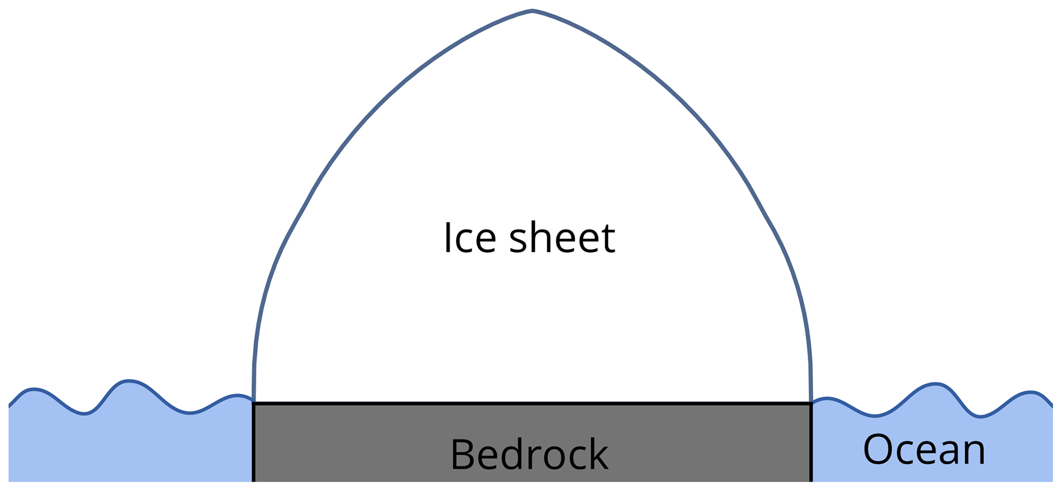
Figure 1 Sketch of the flow-line setup. The ice is sitting on a flat bed; the fixed calving front does not allow ice shelves. The accumulation rate is constant throughout the simulation domain, and the temperature is altitude dependent.

The model is initialized with a spatially constant ice thickness and is run into equilibrium for different combinations of flow parameters Q_c,Q_w, and n. The ice surface temperature is altitude dependent, $T_{\text{s}}=-\mathrm{6}{}^{\circ }\mathrm{C}{\mathrm{km}}^{-\mathrm{1}}\cdot z-\mathrm{2}{}^{\circ }\mathrm{C}$, where z is the surface elevation in kilometers. The accumulation rate is constant in space and time for each simulation. A constant geothermal heat flux of 42 mW m⁻² is prescribed. In the warming experiments, for each ensemble member an instantaneous temperature increase of $\mathrm{\Delta }T\in [\mathrm{1},\mathrm{2},\mathrm{3},\mathrm{4},\mathrm{5},\mathrm{6}]$ ^∘C is applied to the ice surface for a duration of 15 000 years (until a new equilibrium is reached), while the climatic mass balance remains unchanged. That means the temperature increase can lead to an acceleration of ice flow but is prohibited from inducing additional melt. This idealized forcing allows us to disentangle the effect of warming on the ice flow from climatic drivers of ice loss.

The thickness profile of the equilibrium state is similar to the Vialov profile (see e.g. Cuffey and Paterson, 2010; Greve and Blatter, 2009). However, in contrast to the isothermal Vialov profile, here the temperature of the ice is allowed to evolve freely, leading to a non-uniform softness of the ice (PISM authors, 2018). The extent in the x direction is given by the geometry of the setup, a flat bed with a calving boundary condition at the margin, and the height and shape of the ice sheet depend on the flow parameters n, Q_w, and Q_c and the accumulation rate a.

3 Results

3.1 Effect of activation energies in model simulations compared to analytical solution

In order to gain a deeper understanding of the influences of Q_c and Q_w on the equilibrium shape of ice sheets, we here compare the simulated results to analytical considerations based on the Vialov profile.

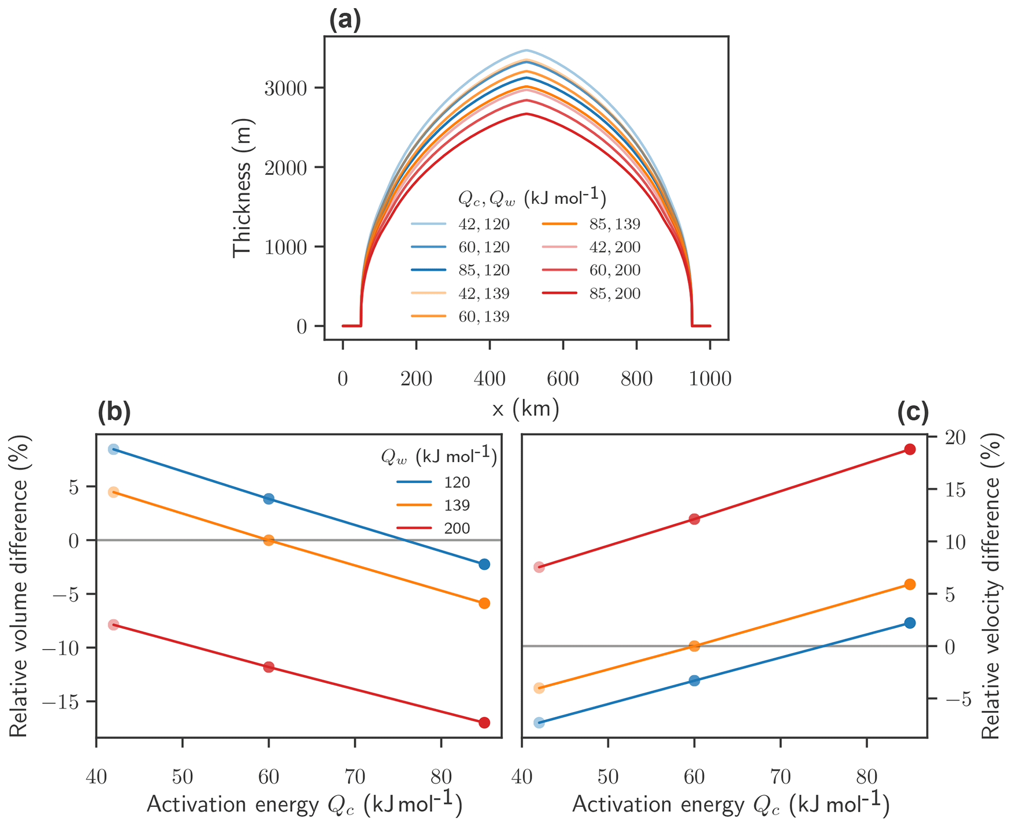
Figure 2 Effect of activation energies on equilibrium volume and velocities with fixed accumulation rate a=0.5 m yr⁻¹ and flow exponent n=3. Thickness profiles of equilibrium states for different combinations of activation energies Q_w and Q_c (a). Relative difference of average equilibrium volumes (b) and velocities (c) compared to the reference state with standard parameters for parameter combinations of Q_w and Q_c. Q_c is shown on the x axis, and Q_w is given through the color of the markers (blue: Q_w=120 kJ mol⁻¹; orange: Q_w=139 kJ mol⁻¹; red: Q_w=200 kJ mol⁻¹).

At a fixed accumulation rate of a=0.5 m yr⁻¹, each flow parameter combination leads to an equilibrium state with a thickness profile similar to the Vialov profile but differences in maximal thickness and volume (Fig. 2a). Overall, high activation energies increase ice-flow velocities and reduce the ice-sheet volume. The activation energy for warm ice, Q_w, affects the volume and the velocities more strongly than the activation energy for cold ice, Q_c. A high Q_w leads to softer ice close to the pressure melting point (Fig. S1) and at the base of the ice sheet, which leads to higher velocities and a lower equilibrium volume of the ice sheet, while a low Q_w leads to stiffer ice close to the pressure melting point and at the base of the ice sheet, and in consequence the velocities decrease and the volume increases (Fig. 2b and c). For a fixed Q_w, the volume appears to decrease linearly with increasing Q_c and the velocity appears to increase linearly with increasing Q_c.

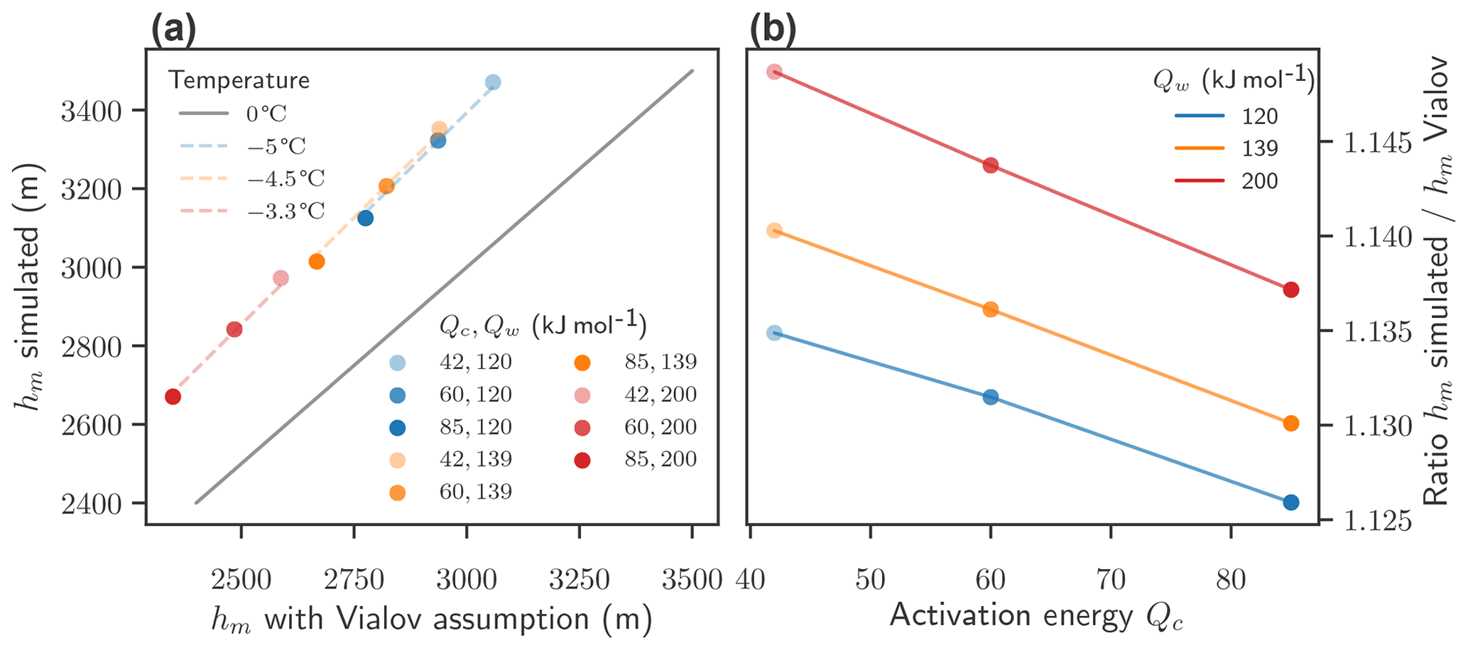
Figure 3 Comparison of simulated equilibrium thickness with analytical results. (a) Dots: maximal thickness h_m of the simulated polythermal ice sheet versus the analytical solution for the maximal thickness h_m of a temperate Vialov profile with the same flow parameters and accumulation rate. Colors indicate the flow–parameter combination. The grey line indicates identity. Short dashed lines indicate the analytical h_m with a temperature lower than the pressure melting point versus h_m at the pressure melting point with the same flow parameters and accumulation rate. The temperature, which fits the simulated results best, is indicated in the legend. (b) Ratio of the simulated h_m to the analytic h_m (assuming a temperate ice sheet) versus Q_c for different parameter combinations of Q_c and Q_w. The value of Q_w is indicated by the color.

The maximal thickness of an isothermal ice sheet can be estimated with the Vialov profile:

$$\begin{array}{}\text{(9)}& {\displaystyle }{h}_{\text{m}}={\mathrm{2}}^{n/(\mathrm{2}n+\mathrm{2})}{L}^{\mathrm{1}/\mathrm{2}}\left({\displaystyle \frac{(n+\mathrm{2})a}{\mathrm{2}A\left(T^{\prime }\right)(\mathit{\rho }g{)}^n}}\right),\end{array}$$

with the Glen exponent n, the ice-sheet extent 2L, the pressure-adjusted temperature T^′, the gravity g, and the ice density ρ (Greve and Blatter, 2009). The Vialov thickness of a temperate ice sheet (isothermal at the pressure melting point), where the softness is evaluated at the pressure melting point depending on the activation energies Q_c and Q_w (see Eq. 2), gives a lower bound to the thickness, given the same geometry and flow parameters. The simulated maximal thickness is larger than the lower bound for all parameter combinations (Fig. 3a, lower bound indicated by a grey line), and the ratio between the maximal thickness h_m from the PISM simulation to the lower bound from the Vialov profile depends on both Q_w and Q_c. The ratio increases with higher Q_w and decreases with higher Q_c (Fig. 3b). The ice-sheet thickness of the polythermal ice sheet, as simulated with PISM, matches well the Vialov thickness calculated with Eq. (9) if an effective temperature $T_{\text{eff}}^{\prime }<\mathrm{0}$ ^∘C is assumed. The effective temperature $T_{\text{eff}}^{\prime }$ that matches simulations best varies for different Q_w. For Q_w=120 kJ mol⁻¹, an effective temperature of $T_{\text{eff}}^{\prime }=-\mathrm{5}$ ^∘C matches well the equilibrium thickness of the polythermal ice sheets. For Q_w=200 kJ mol⁻¹, an effective temperature of $T_{\text{eff}}^{\prime }=-\mathrm{3.3}$ ^∘C matches well the equilibrium thickness of the polythermal ice sheets. These differences can be partly explained by the altitude-dependent surface temperature: the maximal thickness of the ice sheets varies by approximately 800 m, which leads to a difference in ice surface temperature of approximately 4.8 ^∘C between the thickest and the thinnest ice and thus influences the temperature within the ice sheet.

The relative difference of average velocities $d_{\text{v}}=(\stackrel{\mathrm{‾}}{v}-{\stackrel{\mathrm{‾}}{v}}_{\mathrm{0}})/{\stackrel{\mathrm{‾}}{v}}_{\mathrm{0}}$ spans from $d_{\text{v}}=-\mathrm{7}$ % (with a corresponding relative difference in ice-sheet volume of $d_{\text{vol}}=+\mathrm{10}$ %) for the lowest combination of activation energies to $d_{\text{v}}=+\mathrm{18}$ % with a difference in volume of $d_{\text{vol}}=-\mathrm{15}$ % for the highest combination of values for Q_c and Q_w (Fig. 2b).

Figure 4 Effect of flow parameters on equilibrium state without warming with adapted accumulation rates and flow exponent n=3. (a) Thickness profile of equilibrium states for parameter combinations of Q_w and Q_c, with a zoom on the ice divide (b). Relative difference of accumulation rates (c) needed to keep the ice-sheet volume in equilibrium close to the reference simulations with standard flow parameters and relative difference in average surface velocities (d) versus Q_c. The value of Q_w is given by the color.

3.2 Ice-sheet initial states

In order to keep the initial ice volume largely fixed (with variations of less than 1 %) in the warming experiments, we adapt the accumulation rate for each parameter combination of Q_c and Q_w.

Since simulations with high activation energies Q_w have a smaller equilibrium volume at the same accumulation rate than simulations with standard activation energies, the accumulation rate a is increased to maintain an equilibrium volume close to the reference value. Simulations with low activation energies Q_c have a higher volume at the same accumulation rate, so the accumulation rate a is decreased. In the case of an isothermal ice sheet the maximal thickness and the volume can be computed analytically as shown above in Eq. (9). In our model simulations, however, the temperature distribution within the ice can evolve freely; thus the softness is not uniform and an analytical solution cannot be found.

In order to find the right adaptation for the accumulation rates, we start from the ice profile from the isothermal approximation as a first guess and run the model into equilibrium. If the relative difference between the new equilibrium volume and the standard equilibrium volume exceeds 1 %, we further change the accumulation rate and repeat the equilibrium simulation, always starting from the same initial state. The final equilibrium states found via this iterative approach differ by a maximum of 0.8 % in ice volume (Fig. S2), and the difference in maximal thickness is less than 100 m (Fig. 4a and b).

For the combination of high activation energies Q_w and Q_c, the relative differences $d_x=(x-x_{\mathrm{0}})/x_{\mathrm{0}}$ of both adapted accumulation rates a and mean surface velocities v increase by more than 300 % (Fig. 4c and d), and for the combination of low activation energies Q_c and Q_w both adapted accumulation rates a and surface velocities v are approximately 50 % lower compared to the case with standard parameters. Both the accumulation rate and the velocities change in the same way since they balance each other in equilibrium. A change in accumulation rates controls the vertical velocity profile and thus influences the thermodynamics in the ice, which leads to differences in the temperatures of the ice sheet (pressure-adjusted temperature distributions shown in Fig. S4a). The change in temperature is most prominent at the top of the ice sheet, where higher accumulation rates (associated with high activation energies) lead to lower temperatures and vice versa. Thus the temperature change introduced from increased accumulation counteracts the effect of increased softness. In order to estimate how changed temperature on the one hand and changed flow parameters on the other hand impact the resulting ice softness, either one was kept fixed. The effect of the temperature changes on the ice softness is negligible, compared to parameter changes (see Fig. S4b, c, and d).

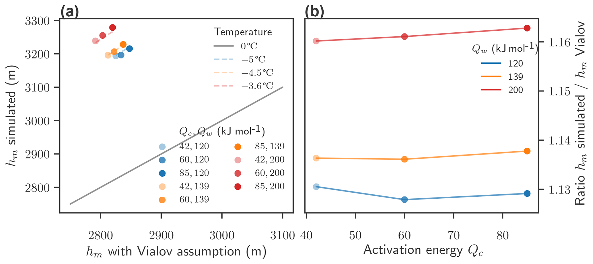
Figure 5 Comparison of simulated equilibrium thickness with analytical results. (a) Dots: maximal thickness h_m of the simulated polythermal ice sheet versus the analytical solution for the maximal thickness h_m of a temperate Vialov profile with the same flow parameters and accumulation rate. Colors indicate the parameter combination. The grey line indicates identity. Short dashed lines indicate the analytical h_m with a temperature lower than the pressure melting point versus h_m at the pressure melting point with the same flow parameters and accumulation rate. The temperature which fits the simulated results best is indicated in the legend. (b) Ratio of the simulated h_m to the analytic h_m (assuming a temperate ice sheet) versus Q_c for different parameter combinations of Q_c and Q_w. The value of Q_w is indicated by the color.

The maximal thickness of the polythermal simulated ice sheet is approximately 13–16 % larger than the lower bound estimated with a temperate ice sheet (Fig. 5a and b) with the same flow parameters and accumulation rates. Similar to the case with fixed accumulation rates, the simulated thickness matches the Vialov thickness well if an effective temperature ${T^{\prime }}_{\text{eff}}<\mathrm{0}$ ^∘C is assumed. The effective temperature that matches simulations best varies for different Q_w, from −5 ^∘C for Q_w=120 kJ mol⁻¹ to −3.6 ^∘C for Q_w=200 kJ mol⁻¹. This difference cannot be sufficiently explained by variations in surface temperature due to the difference in ice-sheet thickness. Rather the higher effective temperatures are linked to increased flow velocities of the ice, which in turn might lead to strain heating. In simulations with a high Q_w the simulated thickness has a higher discrepancy to the estimated lower bound (assuming a temperate ice sheet) than simulations with a low Q_w. In contrast to the case with fixed accumulation rate (Fig. 3) the ratio between the estimated and the simulated thickness depends only very little on Q_c.

3.3 Flow-driven ice loss under warming

Disentangling the purely flow-driven ice losses from the influences of melting, different initial temperature profiles, and variations in sliding requires several conditions:

1. The initial volume is fixed, which here is attained through adjustment of the accumulation rate for the different flow parameter combinations as explained in Sect. 3.2.

2. The surface mass balance is fixed – i.e., we do not allow for additional melt – and the accumulation rate does not change with warming.

3. Sliding is effectively inhibited (which is here ensured by applying an SIA-only condition).

The effect of the temperature increase is limited to warming at the ice surface, which can propagate into the interior of the ice sheet through diffusion and advection. Warming makes the ice softer and thus accelerates the flow and ice discharge. Since temperature diffusion in an ice sheet is a very slow process, we apply the temperature anomaly for a total duration of 15 000 years. The total mass balance is evaluated and compared to the standard parameter simulation after 100, 1000, and 10 000 years of warming. A new equilibrium state is reached after 10 000 years for all parameter combinations (see longer time series in Fig. S3).

Figure 6 Time series for flow-driven ice discharge under 2 ^∘C warming: (a) time evolution of ice loss with different activation energies Q_c and Q_w and the flow exponent n=3, subject to a temperature anomaly forcing of ΔT=2 ^∘C. (b) Zoom on the first 100 years.

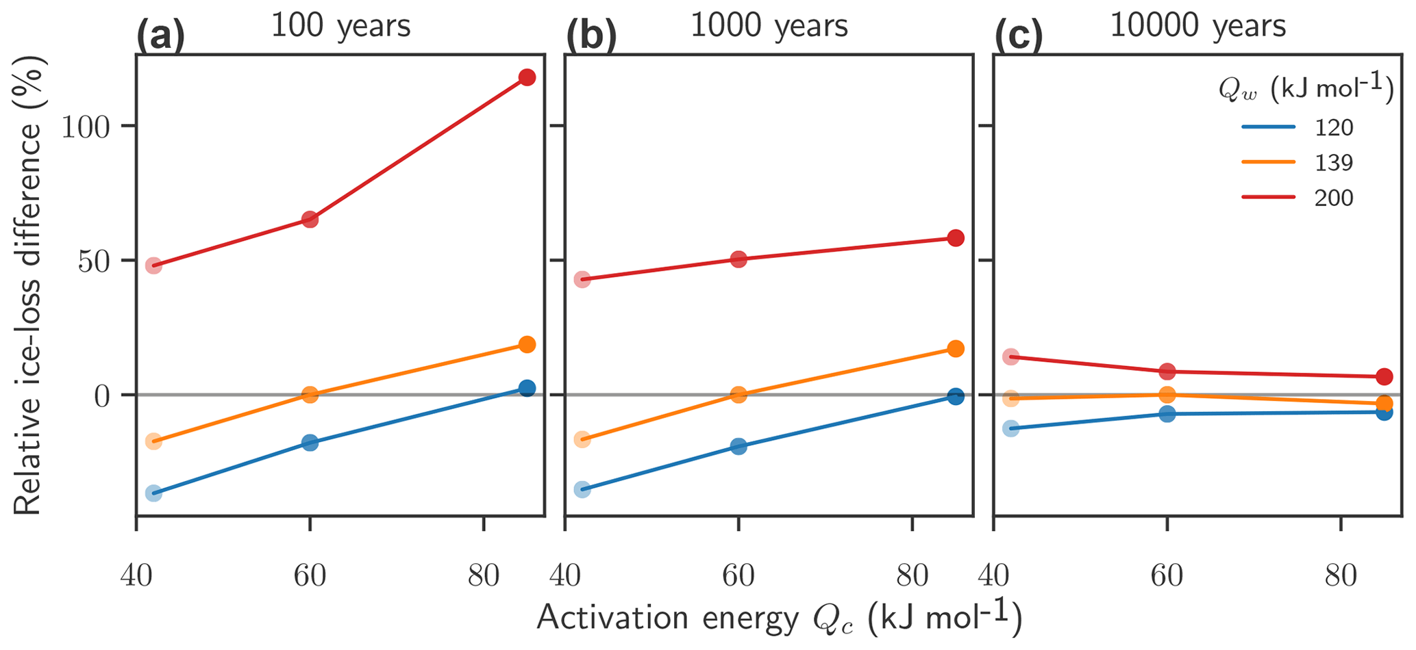
Figure 7 Effect of activation energy on flow-driven ice discharge under 2 ^∘C warming: relative difference of flow-driven ice loss after 100 (a), 1000 (b), and 10 000 (c) years versus Q_c. The value of Q_w is given by the color. The simulations have reached a new equilibrium after 10 000 years.

In the experiments, the ice sheet loses mass for all warming levels and all parameter combinations. However, the amount and rate of the ice loss are dependent on the flow parameters. Figure 6 shows the ice-sheet response to a warming of 2 ^∘C. For a fixed flow exponent of n=3 the fastest ice loss is observed for the flow parameter combination of Q_c=85 kJ mol⁻¹ and Q_w=200 kJ mol⁻¹, and the slowest ice loss for Q_c=42 kJ mol⁻¹ and Q_w=120 kJ mol⁻¹. Simulations with Q_w=200 kJ mol⁻¹ reach a new, temperature-adapted equilibrium after only 2000 years, while simulations with lower Q_w continue to lose mass.

The sensitivity to variations in flow parameters is measured via the relative differences for flow-driven ice loss $d_m=(\mathrm{\Delta }m-\mathrm{\Delta }{m}_{\mathrm{0}})/\mathrm{\Delta }{m}_{\mathrm{0}}$, where the reference Δm₀ is always given by the simulation with standard parameters under the same temperature increase (Fig. 7). While the long-term response to warming, after 10 000 years, is not very sensitive to the particular choice of flow parameters, the rate of flow-driven ice loss is. The largest relative differences in ice loss is found in the first century after the temperature increase (Fig. 7a), indicating that high Q_w speeds up the flow-driven ice loss. Under 2 ^∘C of warming, ice loss after 100 years is enhanced more than 2-fold (i.e., increased by up to 118 %) in simulations with Q_w=200 kJ mol⁻¹, while low Q_w reduces the relative ice loss by up to 37 %.

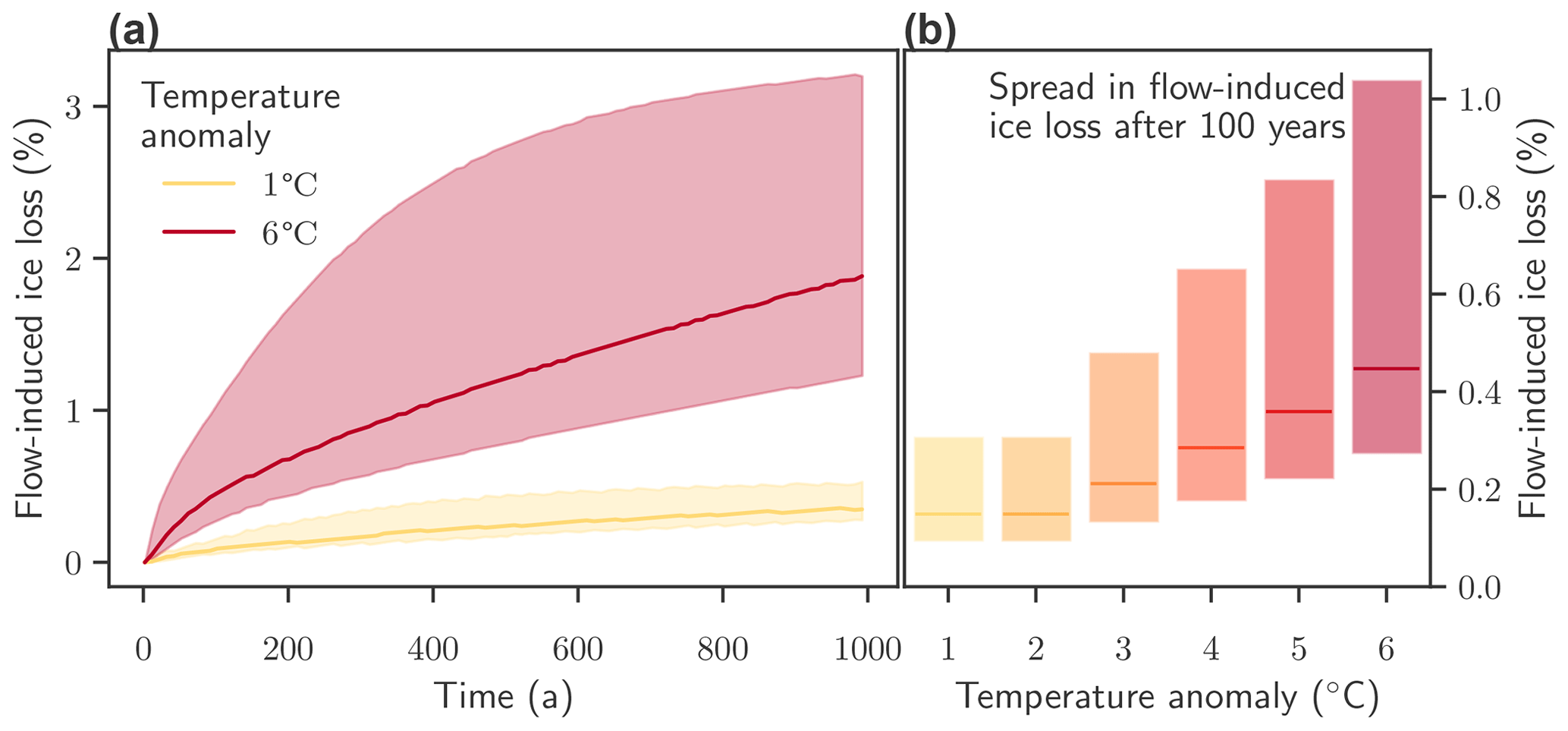
Figure 8 Effect of temperature forcing and activation energy on flow-driven ice. (a) Time evolution of ice loss under warming of 1 ^∘C and 6 ^∘C. For warming of ΔT=1 ^∘C the conceptual ice sheet loses 0.35 % of ice after 1000 years for standard parameters (solid yellow line). Variations in the activation energies Q lead to variations in ice loss on the same order of magnitude (shaded area). For a warming of ΔT=6 ^∘C the conceptual ice sheet loses 1.89 % of ice after 1000 years for standard parameters (solid red line). The variations in ice loss due to different parameters for the activation energy Q (shaded area) are strongly asymmetrical and, in particular during the first 300 years, high compared to the total amount of ice loss. (b) Uncertainty in flow-induced ice loss after 100 years of simulation time over all combinations of Q_w and Q_c, and temperature anomalies ΔT. The flow exponent n=3 is kept fixed for all simulations.

The effect of the flow parameters on flow-driven ice loss upon warming is robust for different temperature increases. Ice losses and the spread in flow-driven ice loss both increase for higher warming levels (see Fig. 8). For a warming of ΔT=1 ^∘C the idealized ice sheet loses 0.09 % after 100 years and 0.35 % of ice after 1000 years for standard parameters. For a warming of ΔT=6 ^∘C the ice sheet loses 0.46 % after 100 years and 1.89 % of ice after 1000 years for standard parameters (solid red line). For comparison, the Greenland Ice Sheet lost approximately 0.18 % of its mass in the period between 1972 and 2018 (Mouginot et al., 2019), which includes all processes: increase in flow, melting, and sliding.

The effect of flow parameter changes on the purely flow-driven ice loss after 100 years is on the same order of magnitude as the effect of surface warming by several degrees. In particular the uncertainty ranges of ice loss for warming of 2 ^∘C and warming of 6 ^∘C overlap (Fig. 8b) when solely considering the ice loss driven by changes in flow and excluding surface mass balance changes.

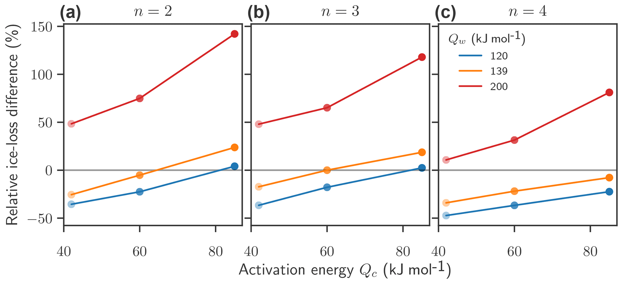
Figure 9 Effect of the flow exponent and activation energies on flow-driven ice loss after 100 years under 2 ^∘C of warming: relative difference in flow-driven ice discharge for n=2 (a), n=3 (b), and n=4 (c) for different combinations of the flow exponent n and activation energies Q_c and Q_w. The reference is always a simulation performed with standard parameters n=3, Q_c=60 kJ mol⁻¹, and Q_w=139 kJ mol⁻¹.

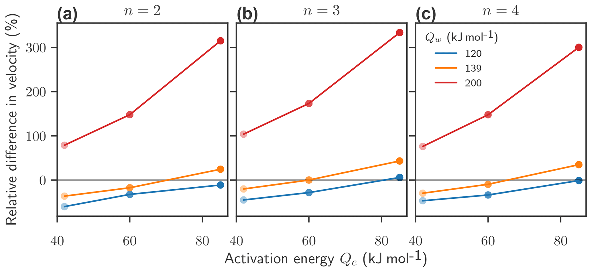
Figure 10 Effect of the flow exponent and activation energies on mean velocity change after 100 years under 2 ^∘C of warming: relative difference in average surface velocity f or n=2 (a), n=3 (b), and n=4 (c) for different combinations of the flow exponent n and activation energies Q_c and Q_w. The reference is always a simulation performed with standard parameters n=3, Q_c=60 kJ mol⁻¹, and Q_w=139 kJ mol⁻¹. Variations in the flow exponent n do not significantly influence the relative difference of mean velocities after 100 years.

3.4 Influence of the flow exponent n

Variations in the flow exponent n do not change the qualitative effect of variations in activation energies Q on the ice loss. After 100 years for a temperature anomaly of ΔT=2 ^∘C a higher n seems to mitigate the effect of the activation energy on differences in ice loss, while a lower n seems to enhance this effect (Fig. 9). However, the effect of variations in activation energy on the average surface velocity is almost independent of the choice of the flow exponent n (Fig. 10).

The influence of the activation energies Q_c and Q_w on ice flow is similar even with different flow exponents n. This is robust for different warming scenarios from +1 to +6 ^∘C. A higher flow exponent n, which leads to a more pronounced nonlinearity in ice flow, does not enhance but reduces variations in dynamic ice loss. Compared to the nonlinear stress dependency τⁿ in the flow law, the temperature-dependent softness $A\left(T^{\prime }\right)=A_{\mathrm{0}}\cdot \exp (-Q/R{T}^{\prime })$ becomes less important with increasing flow exponent n.

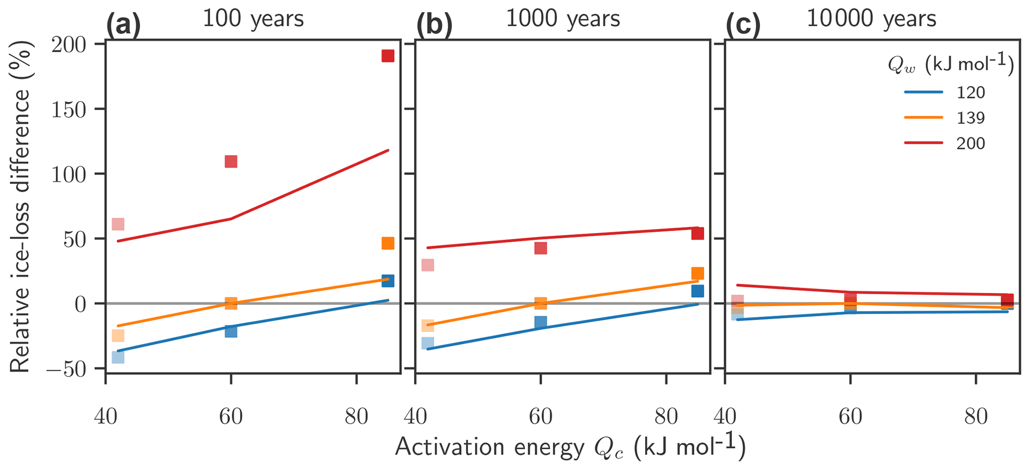
Figure 11 Effect of the flow exponent and activation energies on flow-driven ice loss under 2 ^∘C of ice warming in combination with a 50 % reduction in accumulation rates: relative difference in flow-driven ice discharge after 100 (a), 1000 (b), and 10 000 (c) years. The ice sheet has reached a new equilibrium after 10 000 years. Relative difference for 2 ^∘C warming with an additional reduction of the accumulation rate of 50 % (squares) is compared to the results without changes in the accumulation rate (lines; also see Fig. 7).

3.5 Robustness of results to changes in accumulation and sliding

The overall effect of uncertainties in the activation energies Q remains robust, even if an additional driver of ice loss is taken into account. In a simulation where in addition to warming of 2 ^∘C we also reduce the accumulation rate by 50 %, the ice losses remain dependent on the flow parameters Q_c and Q_w (Fig. 11; lines indicate results without a change in accumulation rate, analogous to Fig. 7, and squares indicate results with an additional 50 % decrease in accumulation rate). After 100 years of forcing, the relative spread of ice loss is slightly larger if accumulation changes are included. In particular, for Q_w=200 kJ mol⁻¹ the relative increase of mass loss mounts from 118 to 190 %. On longer timescales, the spread in ice loss is reduced (after 10 000 years of forcing, when the ice sheet has reached a new equilibrium, the relative spread is below ±10 %).

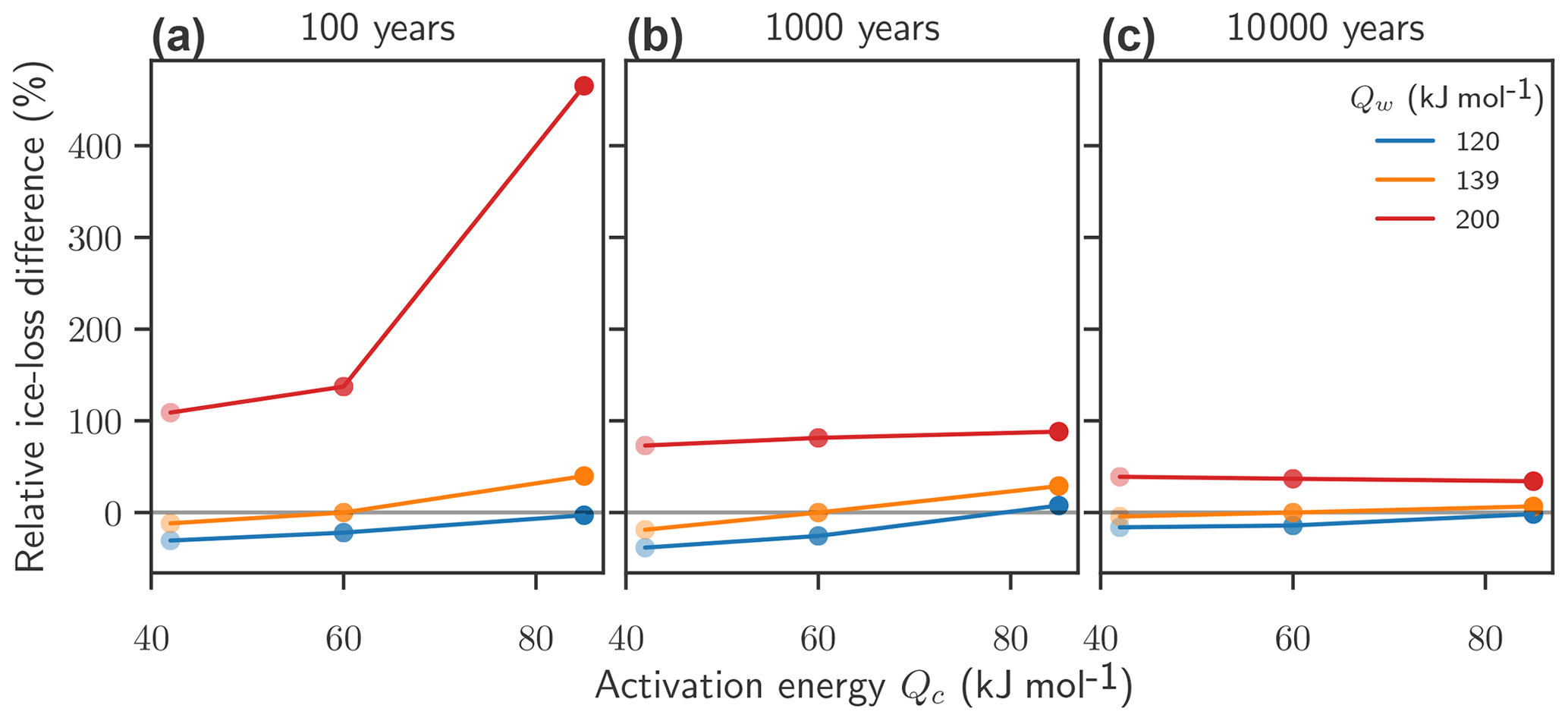
Figure 12 Effect of activation energy on flow-driven ice discharge under 2 ^∘C warming, including sliding: relative difference of flow- and sliding-driven ice loss after 100 (a), 1000 (b), and 10 000 (c) years. The simulations have reached a new equilibrium after 10 000 years.

When sliding is taken into account via the shallow-shelf approximation for sliding ice (see PISM authors, 2018) the uncertainty in flow parameters leads to relative changes in ice loss from −30 to +470 % after 100 years, which is a considerably larger spread than without sliding. The relative differences decrease with time but remain ranger than without sliding. After 1000 years the ensemble member with low activation energies have lost 40 % less ice than the standard parametrization, and high activation energies almost double the ice loss (+90 %). After 10 000 years, when the ice sheets have reached a new equilibrium, the relative differences still range from −16 to +40 % (see Fig. 12).

4 Discussion and conclusion

In this study we present a first attempt to disentangle and quantify the effect of uncertainties in the flow law parameters, in particular the activation energies Q and the flow exponent n, on ice dynamics.

The effect of ice rheology in ice-sheet models has been addressed in several studies with different experimental setups and different time frames. In particular the effect of the enhancement factors, which are often used to approximate the change in ice flow due to anisotropy, has been explored (Ritz et al., 1997; Ma et al., 2010; Humbert et al., 2005; Quiquet et al., 2018). In addition, the effect of the initial conditions (Seroussi et al., 2013; Nias et al., 2016; Humbert et al., 2005) and the effect of the mathematical form of the flow law itself (Quiquet et al., 2018; Peltier et al., 2000; Pettit and Waddington, 2003) have been studied. These studies have been crucial for the understanding of different enhancement factors in the shallow-ice and the shallow-shelf approximation (Ma et al., 2010), for the reconciliation of the aspect ratios of the Greenland Ice Sheet and the Laurentide Ice Sheet during the Last Glacial Maximum (Peltier et al., 2000) and the ice flow in Antarctica and the Greenland Ice Sheet (Ritz et al., 1997; Seroussi et al., 2013; Quiquet et al., 2018; Nias et al., 2016; Humbert et al., 2005).

However, the approach presented in this paper is different in two important respects: firstly, the systematic study of not only the flow exponent n but also the activation energies Q has not been performed so far. Secondly, the idealized experimental setup, as presented in this study, allows us to disentangle the effects of the flow itself from other drivers and other sources of uncertainty. Several conditions need to hold to this end: the ice sheet is sitting on a flat bed and its maximal extent is determined by a calving front at the borders of the bed; thus no ice–ocean interactions or impacts of the bed geography influence the ice flow. Sliding is generally inhibited (the ice dynamics are described by the shallow-ice approximation, with zero basal velocity); no changes in sliding velocity influence the ice flow. The accumulation rate is fixed and independent of the temperature change, so that the ice loss is only driven by changes in flow and not by melting. These idealizations allow a clear understanding of the impact of the flow exponent and the activation energies on ice flow. In addition, they allow us to compare the simulations of the polythermal ice sheet to the analytically solvable limit of an isothermal ice sheet by using the Vialov approximation.

In this setup the largest effect of the uncertainties in the flow parameters is observed in the first century after warming, while the effect of the uncertainties on ice loss becomes less important as the ice approaches a new equilibrium. Uncertainties in the activation energies alone account for up to a doubling in ice loss during the first 100 years of warming and are on the same order of magnitude as the effects of increased temperature forcing, under fixed surface mass balance. This effect remains robust, even if changes in the surface mass balance are taken into account. Reducing the surface mass balance by 50 %, which is comparable to the changes in total surface mass balance of the Greenland Ice Sheet from 1972 to 2012 (Mouginot et al., 2019), increases the effect of the flow parameters on a timescale of 100 years and remains comparable on a timescale of 1000 years. Only as the ice sheet approaches its new equilibrium does the effect of the flow parameters become negligible. Allowing for not only flow but sliding while keeping all other conditions equal increases the effect of flow parameters substantially, leading to up to a 5-fold increase in ice loss after 100 years compared with standard parameters.

Acknowledging the uncertainty in flow parameters might slightly shift the interpretation of previous studies. For instance, the effect of the initial thermal regime, as studied by Seroussi et al. (2013), could be enhanced if the activation energies were higher than assumed, by making the ice softness more sensitive to changes in temperature. The crossover stress in the multi-term flow law presented by Pettit and Waddington (2003), at which the linear and the cubic term are of the same importance, is highly sensitive to the values of the activation energies. The positive feedback through shear heating, as studied for example by Minchew et al. (2018), could also be enhanced if activation energies were higher than usually assumed. The uncertainty in the flow law parameters may further provoke a re-evaluation of other parameters, for instance concerning melting and basal conditions. In particular, the thorough analysis by Bons et al. (2018) of observational data on the Greenland Ice Sheet supports a flow exponent of n=4, not the standard value of n=3, which is in line with recent laboratory experiments which also find n>3 (Qi et al., 2017). Assuming a higher flow exponent n=4 has shown to significantly reduce the previously assumed area where sliding is possible (Bons et al., 2018; MacGregor et al., 2016). Moreover, both the flow exponent n and the activation energies Q feed into the grounding line flux formula (Schoof, 2007). In several ice-sheet models, this formula is used to determine the position and the flux over the grounding line in transient simulations (Reese et al., 2018). A change in the flow parameters n and Q thus has implications for the advance and retreat of grounding lines in simulations of the Antarctic Ice Sheet and possibly the onset of the marine ice-sheet instability, a particularly relevant process for the long-term stability of the Antarctic Ice Sheet. On the Greenland Ice Sheet increased ice flow might drive ice masses into ablation regions, where the ice melts. A possible effect of uncertainty in flow parameters on this particular feedback remains to be explored. Aschwanden et al. (2019) have found that uncertainty in ice dynamics plays a major role for mass loss uncertainty during the first 100 years of warming. While their study attributes the uncertainty mostly to large uncertainties in basal motion and only to a lesser extent to the flow via the enhancement factor, the uncertainties of the flow law and of the basal motion are not independent, as suggested for instance by Bons et al. (2018).

While the conclusions from the idealized experiments presented here cannot be transferred directly to assessing uncertainty in sea-level-rise projections, they are an important first step which helps to inform choices about parameter variations in more realistic simulations of continental-scale ice sheets.