the Creative Commons Attribution 4.0 License.
the Creative Commons Attribution 4.0 License.
 | 19 Oct 2020
Toward a method for downscaling sea ice pressure for navigation purposes
Jean-François Lemieux
L. Bruno Tremblay
Mathieu Plante
Sea ice pressure poses great risk for navigation; it can lead to ship besetting and damages. Contemporary large-scale sea ice forecasting systems can predict the evolution of sea ice pressure. There is, however, a mismatch between the spatial resolution of these systems (a few kilometres) and the typical dimensions of ships (a few tens of metres) navigating in ice-covered regions. In this paper, the downscaling of sea ice pressure from the kilometre-scale to scales relevant for ships is investigated by conducting high-resolution idealized numerical experiments with a viscous-plastic sea ice model. Results show that sub-grid-scale pressure values can be significantly larger than the large-scale pressure (up to ∼ 4 times larger in our numerical experiments). High pressure at the sub-grid scale is associated with the presence of defects (e.g. a lead). Numerical experiments show significant stress concentration on both sides of a ship beset in sea ice, especially at the back. The magnitude of the stress concentration increases with the length of the lead (or channel) behind the ship and decreases as sea ice consolidates by either thermodynamical growth or mechanical closing. These results also highlight the difficulty of forecasting, for navigation applications, the small-scale distribution of pressure, and especially the largest values as the important parameters (i.e. the length of the lead behind the ship and the thickness of the refrozen ice) are not well constrained.
- Article
(6454 KB) - Full-text XML
- BibTeX
- EndNote


With the growing shipping activities in the Arctic and surrounding seas, there is a need for user-relevant sea ice forecasts and products at multiple timescales and spatial scales. An important forecast field for navigation is the internal sea ice pressure (simply referred to as pressure for the rest of this paper). In compact ice conditions, high-pressure events can complicate navigation activities and even pose great risk for ship besetting.
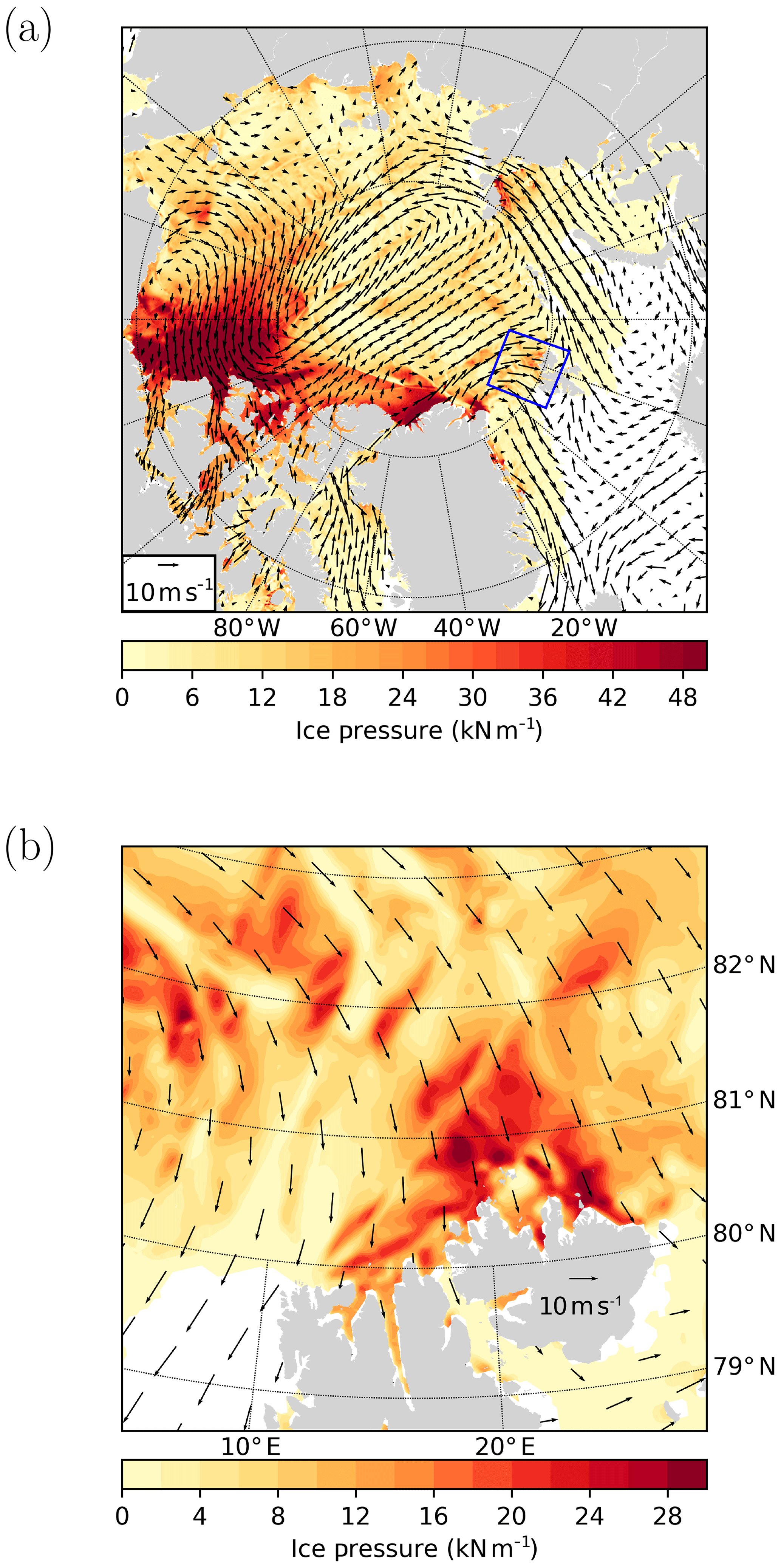
Figure 1A 24 h forecast of the sea ice pressure (kN m−1) and of the surface winds (m s−1) from the Canadian Arctic Prediction System (CAPS). The forecast was initiated at 00:00 UTC on 29 April 2020. Almost all of the domain is shown in (a), while (b) is a subset of the domain located in the region of Svalbard (the sub-region is defined by the blue rectangle in a). Note that the colour scale is not the same for the two panels.
By solving equations for the momentum balance and for the ice thickness distribution, sea ice models are able to predict the evolution of the pressure field. However, even for high-resolution operational forecasting systems with spatial resolutions of a few kilometres (e.g. Dupont et al., 2015; Hebert et al., 2015), there is a clear mismatch in the spatial scales considered. Indeed, the forecast pressure from the model, which represents the average pressure for a grid cell of a few kilometres wide, is not necessarily relevant for a much smaller ship; there are larger pressure values than the average pressure provided by the sea ice forecasting system (Kubat et al., 2010, 2012; Leisti et al., 2011). Figure 1 shows an example of a pressure forecast from a large-scale forecasting system. The Canadian Arctic Prediction System (CAPS) is a fully coupled atmosphere–sea ice–ocean system developed and maintained by the Canadian Centre for Meteorological and Environmental Prediction. Its domain covers the Arctic Ocean, the North Atlantic and the North Pacific. The spatial resolution of the atmospheric model is ∼ 3 km, while the spatial resolution in this region for the sea ice and ocean models is ∼ 4.5 km. Looking at a specific region that is north of Svalbard (Fig. 1b), it can be observed that the surface winds push the ice toward the coast and create large pressure.
Some researchers have done case studies of compressive or besetting events using large-scale sea ice forecasting systems (e.g. Kubat et al., 2012, 2013; Leisti et al., 2011). These besetting events are all associated with heavy ice conditions. The investigations of Kubat et al. show the importance of the coast on pressure conditions; the sea ice pressure often increases toward the coast.
Mussells et al. (2017) used ship logs and satellite imagery to relate besetting events and density of sea ice ridges. They indeed found that the ship was often beset in areas and times of the year with high ridge densities. Probabilistic models for ship performance in sea ice and likelihood of besetting events have also been developed (e.g. Montewka et al., 2015; Turnbull et al., 2019). Turnbull et al. (2019) argue that the primary cause of the besetting events they studied were the relatively large ice floes encountered by the vessel.
There is also a vast literature on the performance of ships navigating in ice-infested waters and on the estimation of ice resistance, that is the longitudinal forces applied on the ship by the ice (e.g. Lindqvist, 1989; Su et al., 2010; Jeong et al., 2017). These calculations are important for ship design and for operational considerations. Lindqvist (1989) introduced a simple empirical formulation to calculate ice resistance based on a ship's characteristics and ice physical parameters. When sea ice pressure is not considered, the resistance encountered by a ship only depends on processes such as crushing, breaking and displacement of ice floes by the ship's hull. Based on laboratory experiments in ice tanks, Kulaots et al. (2013) extended this empirical approach by also considering the effect of compression on the performance of ships navigating in ice-infested waters. There are also some numerical studies of ice loads on ships transiting in ice-infested waters where sea ice is represented using discrete elements (i.e. the floes; Metrikin and Løset, 2013; Daley et al., 2014) or as a continuum (e.g. Kubat et al., 2010).
In contrast with studies mentioned in the last paragraph, we focus on ship besetting rather than on a ship progressing in an ice-covered region. We also study the downscaling of sea ice pressure from the kilometre scale to scales relevant for navigation activities (tens of metres). Note that this was briefly investigated by Kubat et al. (2010) for a ship transiting through a loose sea ice cover. Kubat et al. (2010) showed that the pressure on the hull of the ship can be 2 orders of magnitude larger than the large-scale pressure. For our numerical experiments, we use a continuum-based viscous-plastic sea ice model. In a first set of simulations, we study how the small-scale pressure depends on the stresses applied at the boundaries, on the ice conditions and on the rheology parameters. The second part of the results is dedicated to shipping applications; we investigate the small-scale pressure field in the vicinity of an idealized ship beset in heavy ice conditions and under compressive stresses. Idealized sea ice modelling studies with a continuum-based approach have been conducted by specifying strain rates at the boundaries (e.g. Kubat et al., 2010; Ringeisen et al., 2019) or by specifying wind patterns (e.g. Hutchings et al., 2005; Heorton et al., 2018). However, to our knowledge, it is the first time that internal stresses are specified at the boundaries.
This paper is structured as follows. In Sect. 2, the sea ice momentum equation and the viscous-plastic rheology are described. The sea ice model used for the numerical experiments is presented in Sect. 3. The approach for prescribing sea ice stresses at the boundaries is presented in Sect. 4. The validation of our experimental setup is done in Sect. 5. The main results are given in Sect. 6. Finally, concluding remarks are provided in Sect. 7.
The large-scale sea ice forecasting system solves the sea ice momentum given by
where ρ is the density of the ice; h is the ice volume per unit area (sometimes referred to as the mean thickness); is the total derivative; f is the Coriolis parameter; is the horizontal sea ice velocity vector; , and are unit vectors aligned with the x, y and z axis of our Cartesian coordinates; τa is the wind stress, τw is the water stress; σ is the internal ice stress tensor with components σij acting in the jth direction on a plane perpendicular to the ith direction; g is the gravitational acceleration; and Hd is the sea surface height. This two-dimensional formulation, which is obtained by integrating along the vertical, is justified when the ratio between the horizontal and vertical scales of the problem is large (i.e. a ratio of at least 10:1; Coon et al., 1974).
The sea ice pressure is by definition the average of the normal stresses, that is
with a negative sign because, by convention, stresses in compression are negative. The pressure is the first stress invariant (i.e. it does not vary with the choice of the coordinate system). The second stress invariant (q), that is the maximum shear stress at a point, is defined by
As the stresses are vertically integrated, the stresses and stress invariants are 2D fields with units of newtons per metre. Because the sea ice stresses are written as a function of the sea ice velocity (see details below), one also obtains the pressure p and the maximum shear stress q when solving the momentum equation for u. Hence, by solving the momentum equation for the large-scale sea ice model, the pressure at every grid point is obtained (we refer to this pressure field as the large-scale pressure).
Here, we consider a small area of sea ice (the size of a grid cell) to be under compressive stresses. The idea is to apply the large-scale pressure at the boundaries of this small area and to simulate the sub-grid-scale sea ice pressure (referred to as the small-scale pressure). We assume here that the ice is neither moving nor deforming (e.g. it is being held against a coast). To further simplify the problem, the wind stress, the water stress, the advection of momentum and the sea surface tilt term are neglected. We wish to find, inside this small domain, the steady-state solution of , which is equivalent to finding the solution of . The stresses are modelled according to the viscous-plastic rheology with an elliptical yield curve (Hibler, 1979). With this rheology, the relation between the stresses and the strain rates can be written as
where δij is the Kronecker delta; are the strain rates defined by , and , ; ζ is the bulk viscosity; η is the shear viscosity; and P is a term which is a function of the ice strength.
The bulk and shear viscosities are, respectively,
where Pp is the ice strength;
; and e is the aspect ratio of the
ellipse, i.e. the ratio of the long and short axes of the elliptical yield curve.
Following Hibler (1979), the ice strength Pp is parameterized as
where P* is the ice strength parameter; A is the sea ice concentration; and C is the ice concentration parameter, an empirical constant set to 20 (Hibler, 1979) such that the ice strength decreases quickly with the ice concentration. Unless otherwise stated, the rheology parameters P* and e are, respectively, set to 27.5 kN m−2 and 2.
When △ tends toward zero, Eqs. (5) and (6) become singular. To avoid this problem, ζ is capped following the approach of Hibler (1979). It is expressed as
where with s−1.
We use a replacement method similar to the one presented in Kreyscher et al. (2000). The P term in Eq. (4) is given by
The replacement method is commonly used in sea ice models to prevent unrealistic deformations of the sea ice cover when there is no external forcing.
The McGill sea ice model is used for the numerical experiments. We use revision 333 with some modifications, described below, for specifying stresses at the boundaries.
Considering a domain of a few kilometres by a few kilometres wide (representing a grid cell of a large-scale sea ice forecasting system), the idea is to use the model at very high resolution for studying the distribution of pressure inside that domain. To do so, the model was modified so that internal stresses can be specified at the boundaries (instead of the usual Dirichlet condition, i.e. u=0, at land–ocean boundaries and the Neumann condition at open boundaries with gradients of velocity equal to 0). These stresses at the boundaries represent the integrated effect of the wind and water stresses (like one would get from a large-scale model). The next section gives more details about the implementation of the stress boundary conditions.
For the experiments, the domain is a square of dimensions 5.12 km×5.12 km. It is subdivided into small squared grid cells of dimensions Δx×Δx, with Δx taking one of the following values depending on the experiment: 10, 20, 40, 80, 160, 320, 640 or 1280 m. The size of the domain was chosen because it is close to the average size of CAPS sea ice grid cells and because 5120 m divided by the Δx listed above gives an integer number of small grid cells. For simplicity, we refer to this domain as our 5 km × 5 km domain.
The momentum equation is solved at time levels Δt, 2Δt, 3Δt, …, where Δt is the time step. We introduce the index , which refers to these time levels. Using a backward Euler approach for the time discretization, the momentum equation is written as
The spatial discretization of Eq. (10) on the McGill model Arakawa C-grid leads to a system of non-linear equations that is solved using a Jacobian-free Newton–Krylov (JFNK) solver (the most recent version is described in Lemieux et al., 2014). The ice starts from rest. The time step is 30 min. At each time level, the non-linear convergence criterion is reached when the Euclidean norm of the residual has been reduced by a factor of 10. The maximum number of non-linear iterations is set to 500. The steady-state solution is assumed when the maximum velocity difference between two time levels is lower than 10−9 m s−1. As the ice is assumed to be held against the coast, the simulated velocities are very small (i.e. most of the ice cover is in the viscous regime). Our numerical simulations therefore provide 2D static fields of the internal stresses inside this small domain. Thermodynamic processes and advection of h and A are neglected for all the numerical experiments described in this paper.
For some of the numerical experiments, a digitized ship is placed inside the domain. The digitized ship is simply defined as a rigid body by using land cells. The boundary conditions on the contour of the ship are therefore no outflow and no slip (i.e. u=0), which is the usual Dirichlet approach for land cells. This allows us to investigate the distribution of small-scale pressure around this idealized ship.
The boundary conditions are imposed the same way on the four sides of the small domain. Hence, to shorten the paper, only the treatment on the west side of the domain is explained here. The McGill model uses an Arakawa C-grid; the center of the cell is the point for tracers (e.g. h and A), while the velocity components are positioned on the left side (for u) and lower side (for v). To avoid confusion with the indices i and j for the stresses σij and the strain rates , the indices l and m are, respectively, used to identify the grid cells along the x and y axes. The cell at the southwesternmost location of the domain has indices l=1 and m=1. Figure 2 shows one of the grid cells in the first column of the domain (on the west side). The left side of the grid cell is on the west boundary of the domain. The sides of the domain are referred to as west (W), east (E), south (S) and north (N).
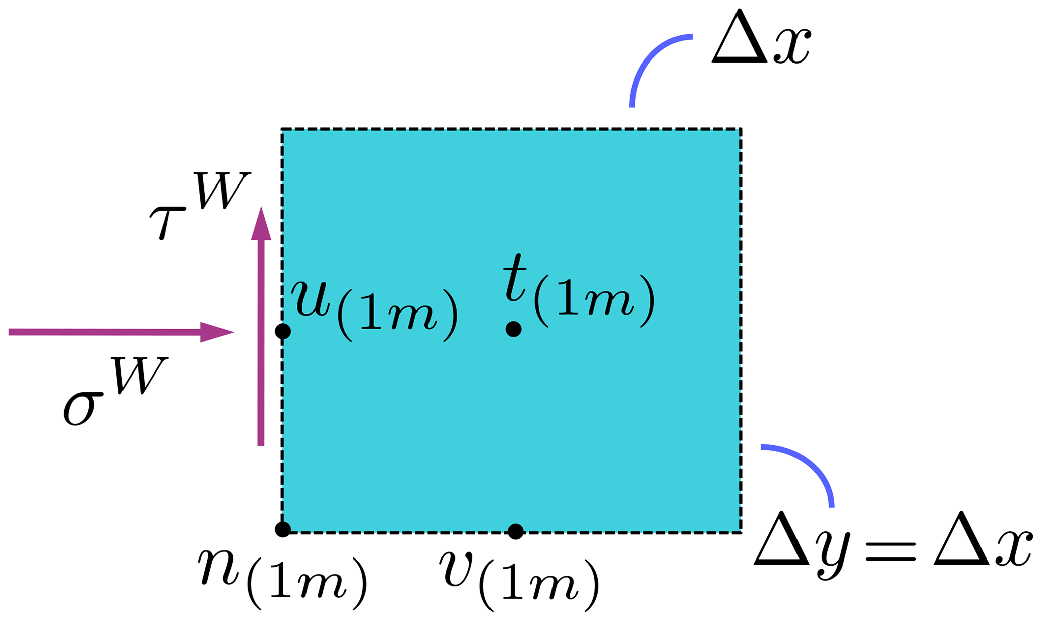
Figure 2One grid cell on the western boundary of the domain with indices l=1 and m. This figure shows the location of the velocity components on the C-grid of the McGill model. The variables h and A are positioned at the tracer point t. Some variables (e.g. σ12) are also calculated at the node (n) point. The stresses (σW and τW) applied at the western boundary are shown with purple arrows.
On the west side of the domain, a normal stress (σW) and a shear stress (τW) are applied. The momentum balance for the u component is comprised of the terms and . Inside the domain, these terms are approximated by second-order centered differences. At the boundaries, however, a one-sided first-order approximation is employed for . Hence, at the u location with l=1 is approximated as
where is evaluated at the t point.
On the other hand, the term only depends on the boundary conditions, that is
For the v component v(1m) (which is at a distance of Δx∕2 from the boundary), there is no special treatment for . However, the second-order treatment of the term follows
where is evaluated at the n point.
Even though u(1m) is located at the boundary, it is solved along with v(1m) and all the other velocity components in the domain by the non-linear solver.
In our simulations, , and ; i.e. they do not vary with m along the boundary (same idea for the other sides of the domain). Furthermore, for numerical stability (see Appendix A), the normal stress on the east side (σE) has to be equal to σW. Similarly, σS=σN and .
The McGill model has, over the years, been extensively tested (e.g. Lemieux et al., 2014; Bouchat and Tremblay, 2017; Williams and Tremblay, 2018). A few simple experiments were conducted in order to validate the implementation of the new stress boundary conditions.
In all the experiments, normal and shear stresses are applied at the four boundaries of the 5 km × 5 km domain. For a given set of sea ice conditions, the steady-state solution of Eq. (10) is obtained. This provides us with the velocity field defined on the Arakawa C-grid. As the stresses and invariants are functions of the sea ice conditions and velocity (see Eqs. 2–9), static 2D fields of the internal stresses and invariants are easily obtained.
Compared to realistic pan-Arctic simulations, the simplicity of the problem allows one to obtain analytical solutions for specific cases. In a first validating experiment, the thickness (h) and concentration (A) fields are, respectively, set to 2 m and 1 everywhere on the domain. By specifying = −10 kN m−1 (i.e. p = 10 kN m−1) and = 0 kN m−1 at the boundaries, the shear stress should be 0 everywhere inside the domain while the pressure field should be constant and equal to 10 kN m−1. This is indeed what is obtained from the numerical experiment (not shown). With p = 10 kN m−1, a 2 m ice cover is able to resist this compressive stress; that is the ice should be in the viscous regime. Using the definition of the stresses from Eq. (4), we obtain , where is the divergence. It is easy to demonstrate that the analytical solution for the divergence is s−1. This is exactly what is obtained with the model (not shown).
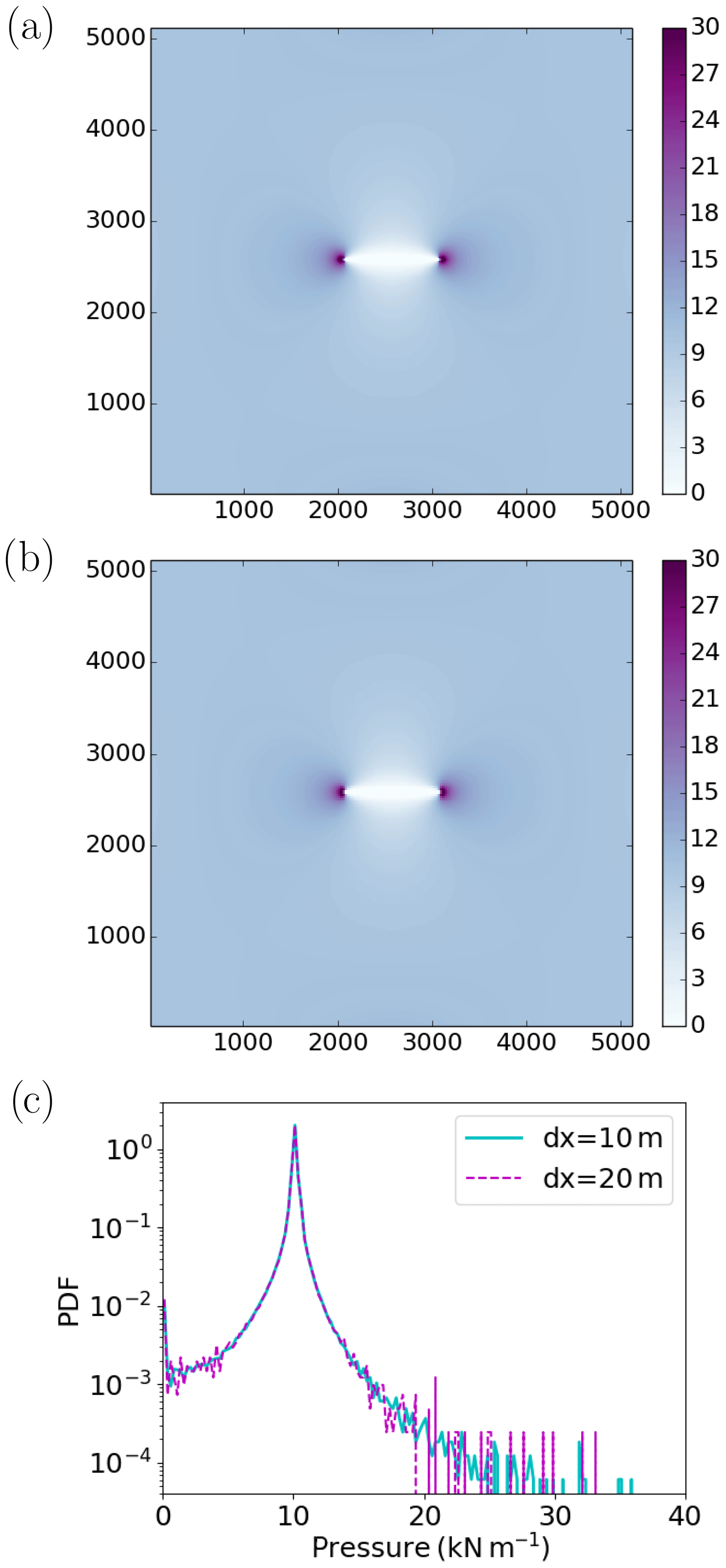
Figure 3Pressure field for Δx = 10 m (a) and Δx = 20 m (b). The thickness field is 2 m everywhere except a 1 km long, 40 m wide horizontal lead in the middle of the domain. The normal stresses at the boundaries are −10 kN m−1. Panel (c) shows PDFs of the pressure in the 5 km × 5 km domain for Δx = 10 m (cyan) and Δx = 20 m (dashed magenta). Bins of 0.25 kN m−1 were used to build the PDFs.
We also verify that we obtain the same results when a lead is present within the physical domain for different spatial resolution (Δx). For example, Fig. 3 shows the pressure field for a 1 km long, 40 m wide lead resolved with a Δx of 10 m (Fig. 3a) and for the same lead resolved with Δx = 20 m (Fig. 3b). The thickness of the level ice (hl) around the lead is 2 m. The maximum pressure at 10 m resolution is 35.79 kN m−1, while the maximum pressure at 20 m is 33.15 kN m−1. From these simulated 2D pressure fields, probability density functions (PDFs) are calculated using bins of 0.25 kN m−1. They are shown in Fig. 3c, which further demonstrates that the simulated fields are very similar at 10 and 20 m resolutions.
The effect of the same lead but oriented differently in the domain was also tested. The PDF of the pressure field is exactly the same whether the lead is oriented horizontally (west–east) or vertically (south–north; not shown). The spatial distribution of pressure is qualitatively the same when orienting the lead diagonally. The PDF of pressure for this diagonal lead is similar to the PDF of the vertical and horizontal ones, although we find that the maximum pressure is usually a bit smaller (not shown). This is likely a consequence of the spatial discretization of a finite width lead on a Cartesian grid.
In a last set of experiments for the validation, we also checked that the presence of relatively nearby boundaries does not affect our conclusions. In the first experiment, with Δx = 20 m, a horizontal 1 km long and 20 m wide lead was positioned in the center of the 5.12 km×5.12 km domain. In a second experiment, again with Δx = 20 m, the same lead was positioned in a domain twice this size; that is the boundaries are much farther from the lead in the second experiment. For both experiments, hl is again equal to 2 m. The pressure fields around the lead are very similar (not shown) in the two experiments, with maximum pressures in the domain equal, respectively, to 36.22 and 36.36 kN m−1 (a difference of ∼ 0.4 %). To avoid these boundary effects, we tend to position the important features in the center of the domain for the numerical experiments. For a numerical experiment to be valid, we require the simulated pressure in the first grid cells around the domain to be within 10 % of the pressure value specified at the boundaries.
To limit the number of parameters that can be varied in the numerical experiments, the thickness of the level ice hl is always set to 2 m. Furthermore, for all the experiments except the ones for the last figure, the normal stresses at the boundaries are always equal to −10 kN m−1, while the shear stresses are set to 0. In other words, = −10 kN m−1 and .
6.1 Idealized sea ice experiments
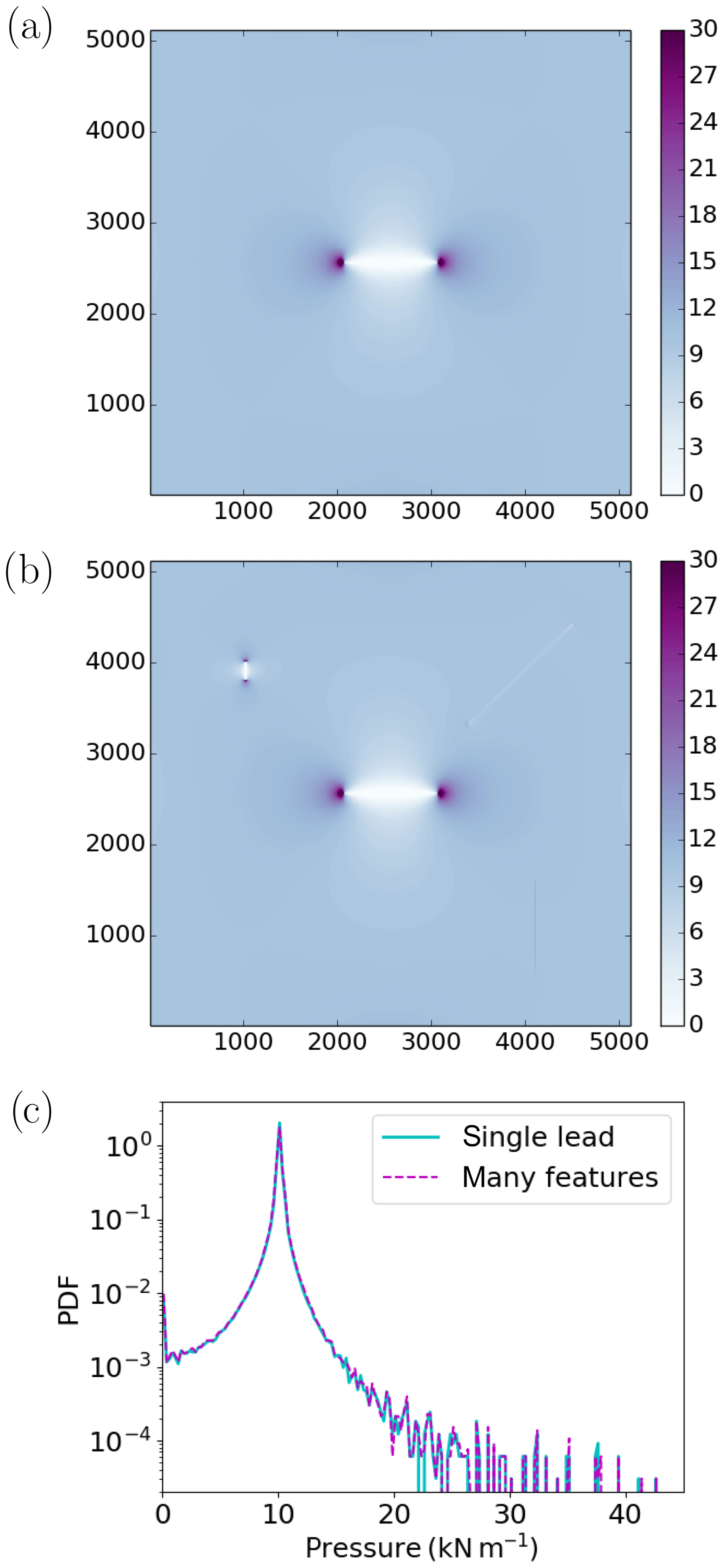
Figure 4Pressure (kN m−1) field for a thickness field of 2 m everywhere except a 1 km long, 10 m wide horizontal lead in the middle of the domain (a; referred to as “single lead”). Pressure (kN m−1) field for a thickness field of 2 m everywhere except a 1 km long, 10 m wide horizontal lead in the middle of the domain, a diagonal refrozen lead (h = 0.5 m), a smaller lead in the northwestern part of the domain and a 1 km ridge (h = 5 m in center, 2.5 m on each side) in the southeastern part of the domain (b, referred to as “many features”). For both experiments Δx = 10 m, and the normal stresses at the boundaries are −10 kN m−1. c PDFs of the pressure for the “single lead” experiment (cyan) and the “many features” experiment (dashed magenta).
In a first set of experiments, we conduct idealized experiments to investigate the impact of sea ice features (leads, ridges, etc.) on the small-scale pressure field and especially on the maximum pressure. These experiments will give us insights and guide us for the second series of experiments with the idealized ship (see Sect. 6.2). Figure 4a shows the pressure field for a uniform sea ice cover with hl=2 m except the presence of a 1 km long and 10 m wide lead. Large pressure is observed at the tips of the lead. In a second experiment, the same sea ice thickness conditions are used except that a smaller lead, a refrozen lead (with h=0.5 m) and a thick sea ice ridge (with h=5 m) are also positioned in the 5 km × 5 km domain. The pressure field for this latter experiment is shown in Fig. 4b. Figure 4c compares the PDFs of pressure for these two experiments. Looking at the PDFs and comparing Fig. 4a and b, one can notice that the other features are not associated with such high pressure values and that the maximum pressure is associated with the long 1 km lead. To further support this conclusion, note that the maximum pressure in the 5 km × 5 km domain is 42.57 kN m−1 in the first experiment, while it is 42.59 kN m−1 in the second one. In other words, the other features do not change our analysis; what really matters is the longest lead as it is in the vicinity of the longest lead that the largest stress concentration is found.
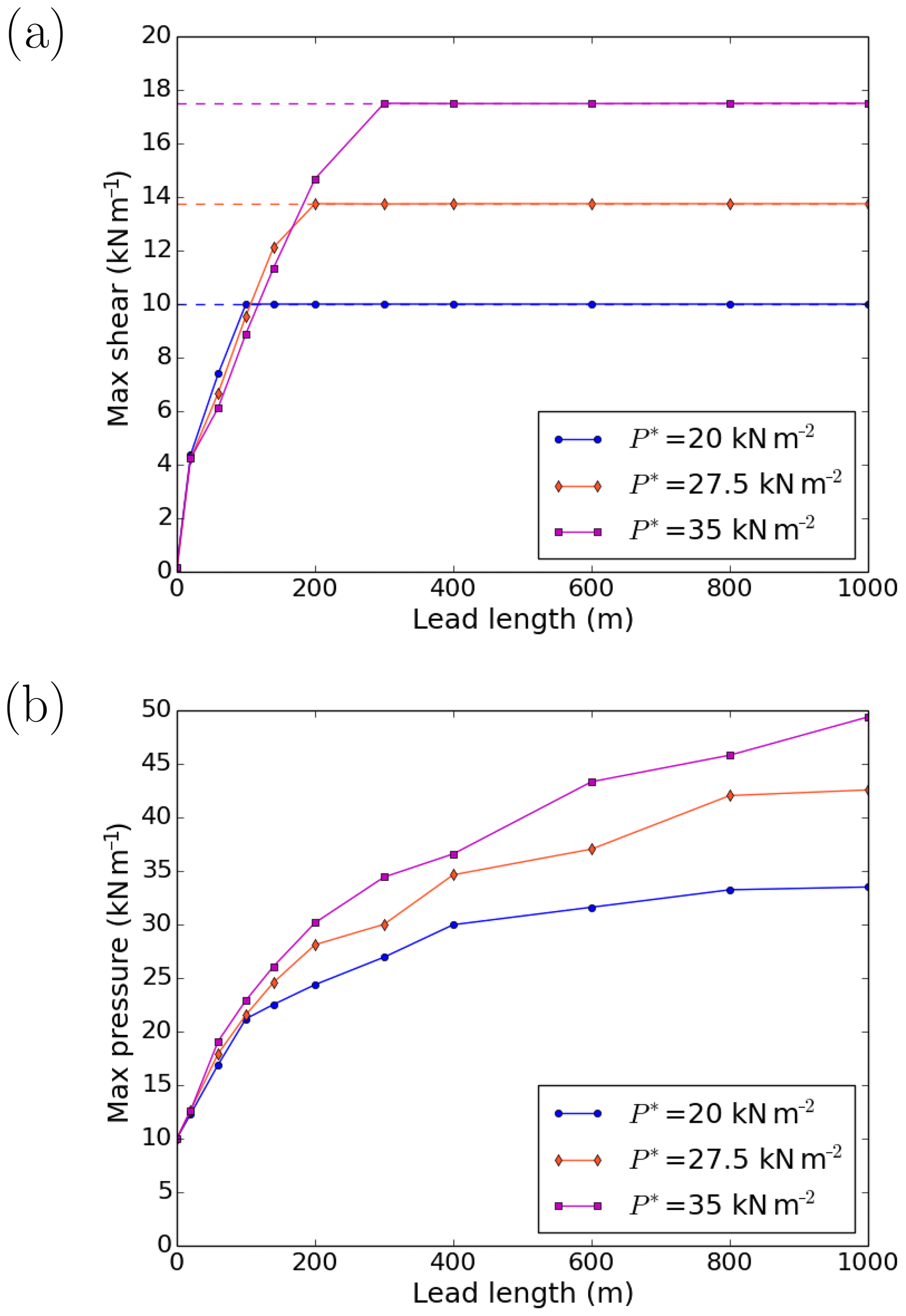
Figure 5Maximum value of the shear stress invariant (a; kN m−1) and of the pressure (b; kN m−1) in the domain as a function of lead length for different values of the parameter P* (P* = 20 kN m−2: blue; P* = 27.5 kN m−2: orange; P* = 35 kN m−2: magenta). The thickness field is 2 m everywhere except the 10 m wide horizontal lead in the middle of the domain. The normal stresses at the boundaries are −10 kN m−1.
Our results above suggest that only the longest lead needs to be considered for estimating the largest small-scale pressure. For a given hl and stresses applied at the boundaries, there is more and more stress concentration when increasing the length of a lead. This is shown in Fig. 5 for three values of the parameter P*. For short leads, the ice around the lead is able to sustain the stresses (the ice is rigid, that is in the viscous regime). This is why the three curves are very similar in Fig. 5a and b for short leads. However, for longer leads, there is more and more stress concentration. Some points of the ice close to the tips of the lead fail (i.e. the state of stress reaches the yield curve).
As the whole yield curve scales with the value of P*, a larger P* leads to larger maximum pressure and shear values. When increasing P*, the maximum shear stress approaches asymptotically the shear strength (dashed lines in Fig. 5a; ). This asymptotic behaviour is less obvious for the pressure (Fig. 5b) as it is still far from the compressive strength (hlP*). A similar behaviour is observed when varying the ellipse aspect ratio (which modifies the shear strength). A smaller value of e leads to larger pressure values and larger shear stresses values (with a similar asymptotic behaviour) for long leads (not shown).
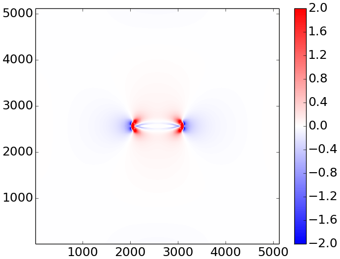
Figure 6Pressure field with P* = 27.5 kN m−2 minus the pressure field with P* = 20.0 kN m−2 (kN m−1). For both experiments, the thickness field is 2 m everywhere except a 1 km long, 10 m wide horizontal lead in the middle of the domain. The normal stresses at the boundaries are −10 kN m−1.
While the average pressure in the domain is the same (10 kN m−1) for all the values of P*, the maximum pressure is enhanced as P* increases (as shown in Fig. 5b). Comparing the pressure fields with P* = 27.5 kN m−2 and P* = 20 kN m−2 (see Fig. 6) for the same lead shows that the pressure fields around the lead are different over hundreds of metres. Moreover, the largest difference in the pressure fields are found at the tips of the lead; the pressure is much larger with P* = 27.5 kN m−2 than with P* = 20 kN m−2 in the vicinity of the tips.
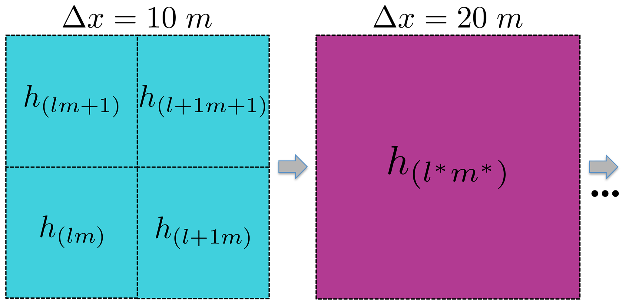
Figure 7Schematic of the coarse-graining procedure. The thickness field is defined at 10 m resolution (blue cells on the left). The thickness field at 20 m resolution is obtained by averaging the h values of the four 10 m cells contained in the 20 m one (purple cell). This procedure is repeated for the other lower resolutions. The same method is applied for the concentration A. The indices l,m are for the 10 m grid, while the indices are for the 20 m grid.
We also investigate the evolution of the small-scale pressure field as a function of resolution. The h and A fields are defined at 10 m resolution. These fields h and A are, respectively, set to 2 m and 1.0 everywhere except for a 1 km long, 10 m wide lead in the middle of the domain with h=0 m and A=0. The model is run at resolutions of 10, 20, 40, … 1280 m. For these lower resolutions, the h and A fields are obtained through a coarse-graining procedure (see Fig. 7 for details).
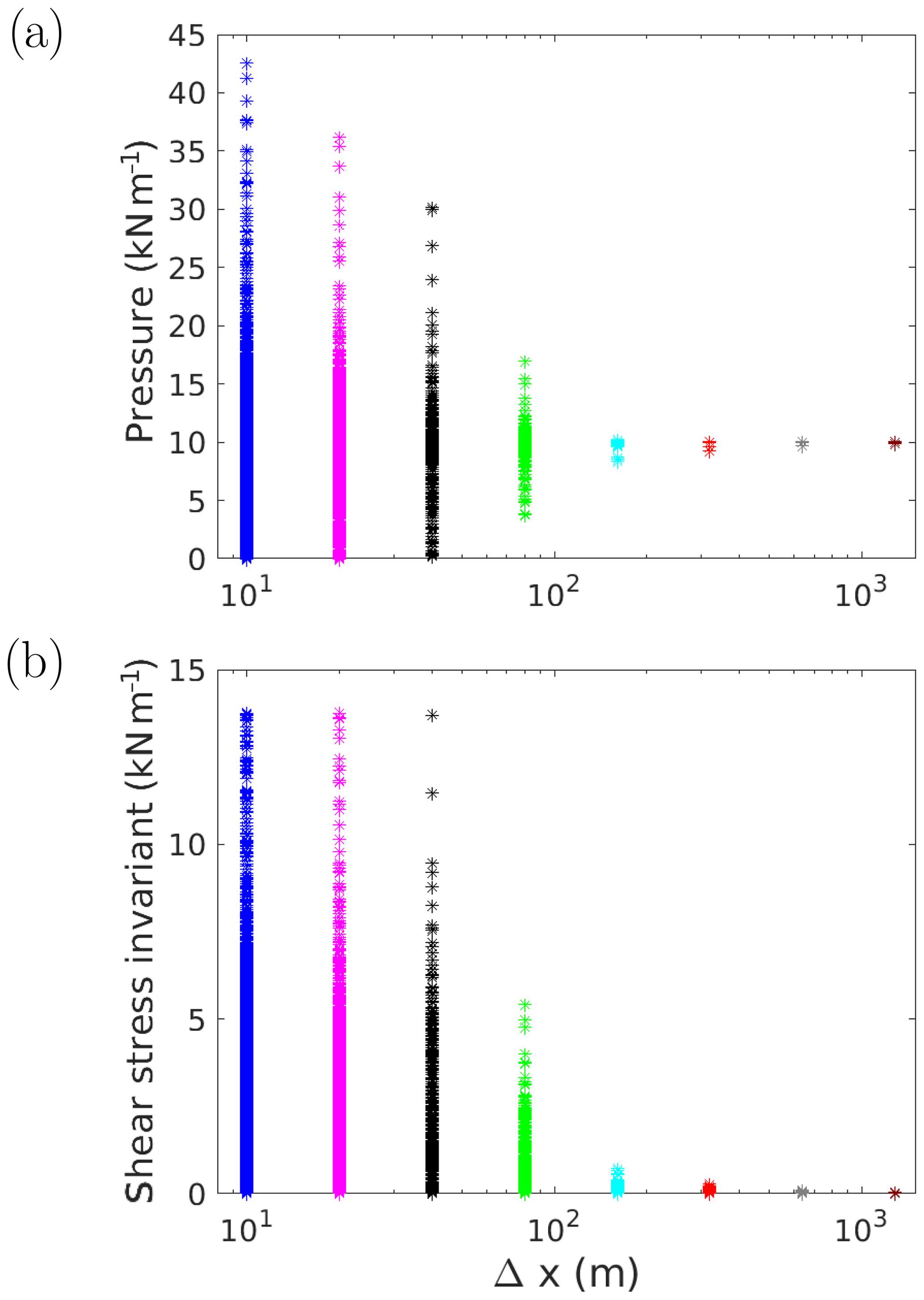
Figure 8All the values of pressure (a) and of the shear stress invariant (b) in the 5 km × 5 km domain as a function of resolution. The thickness field is 2 m everywhere except a 1 km long, 10 m wide horizontal lead in the middle of the domain. The thickness and concentration fields at the other resolutions are obtained through a coarse-graining procedure. The normal stresses at the boundaries are −10 kN m−1.
All the values of p and q in the 5 km × 5 km domain are plotted as a function of Δx in Fig. 8a and b. The distribution of these small-scale stresses are non-symmetric (they are limited by 0 on one side) and are skewed toward large values. These results constitute another validation of the numerical framework as the distribution reduces to a single point equal to the large-scale values prescribed at the boundaries as Δx tends toward the horizontal dimension of the domain.
6.2 Experiments with an idealized ship
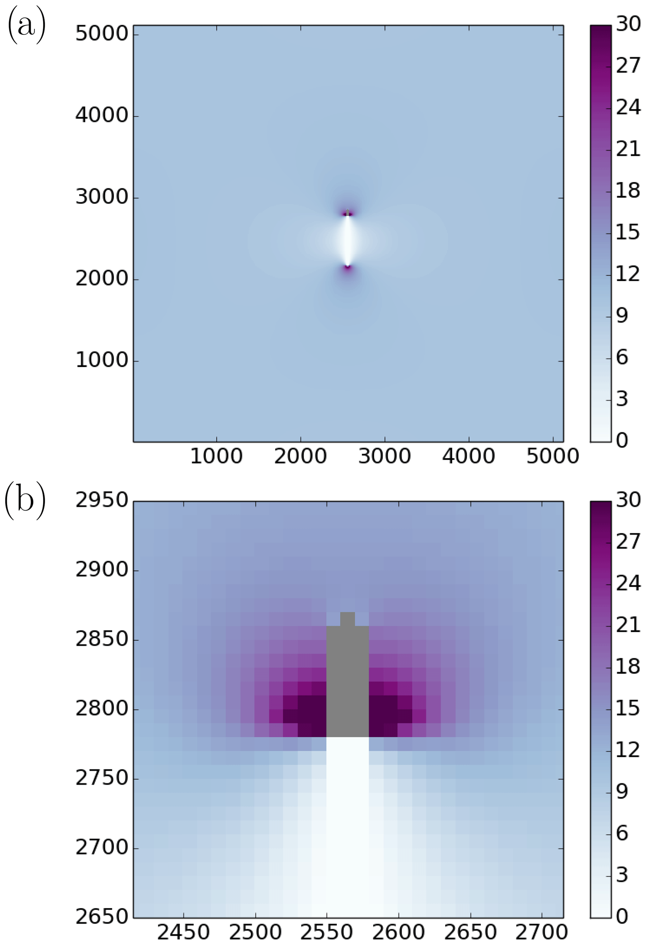
Figure 9Pressure field at 10 m resolution when including a digitized ship 90 m long and 30 m wide (in grey). The thickness field is 2 m everywhere except a 600 m long lead behind the ship. The normal stresses at the boundaries are −10 kN m−1. The whole domain is shown in (a), while (b) shows a zoom of the pressure field around the ship.
In a second set of experiments, we investigate the small-scale pressure field in the vicinity of a ship in heavy sea ice conditions and under compressive stresses. Importantly, we estimate the maximum pressure applied on the ship in different idealized experiments. The small-scale pressure field around a ship 90 m long and 30 m wide is investigated. We assume that the ship was navigating in level ice 2 m thick and that it is now beset. First, it is assumed that a lead (i.e. a channel) created by the ship is still open behind it over a distance of 600 m, while farther away the lead has been closed due to resulting sea ice convergence. The pressure field for this experiment is shown in Fig. 9a and with more details in Fig. 9b. Similar to our previous results without a ship, larger pressures are found at the tips of the lead. In fact, there is very large pressure on both sides of the ship, especially at the back of the ship. Numerical simulations of ships navigating in sea ice show larger pressure at the front of the ship (e.g. Kubat et al., 2010; Sayed et al., 2017). However, our results show the opposite for a ship that is beset. These results also suggest that by navigating in these compact ice conditions, the ship has generated these high-pressure conditions by creating a lead in its wake.

Figure 10Maximum pressure (kN m−1) on the ship as a function of the length of the lead behind the ship. The thickness field is 2 m everywhere except in the lead behind the ship; the thickness of the refrozen lead (hrf) is 0 cm for the blue curve, it is 10 cm for the orange one, and it is 20 cm for the magenta one. The digitized ship is 90 m long and 30 m wide. The normal stresses at the boundaries are −10 kN m−1.
A crucial aspect to consider here is the length of the lead behind the ship. Assuming the lead closes at a shorter distance from the ship should imply smaller pressure values (for the same pressure applied at the boundaries). This is indeed the case as demonstrated by the sensitivity study shown in Fig. 10 (blue curve). We also consider the case of a lead partially consolidated. In fact, we assume that the concentration (A) is 0 just behind the ship and that it increases linearly to 1.0 for a certain lead length. The (mean) thickness h of the ice is set equal to Ahl. This appears to have a very small effect on our results (not shown) compared to the case with A=0 everywhere in the lead (blue curve in Fig. 10). This is due to the fact that the ice strength (see Eq. 7) decreases rapidly as A diminishes. However, if we consider that the ice in the lead is consolidating through thermodynamical growth (i.e. we set h to a small value in the lead behind the ship), we find that this notably reduces the stress applied on the ship. This can be seen with the orange and magenta curves in Fig. 10, which, respectively, correspond to thicknesses of 0.1 and 0.2 m for the refrozen lead.
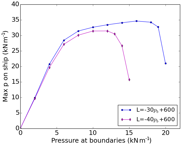
Figure 11Maximum pressure (kN m−1) on the ship as a function of the pressure (pb) prescribed at the boundaries. For both curves, it is assumed that the length of the lead (L) is 600 m for pb = 0 kN m−1 and that it decreases linearly as pb increases. For the blue, the lead behind the ship is closed when pb reaches 20 kN m−1, while the lead is closed when pb = 15 kN m−1 for the magenta curve. The thickness field is 2 m everywhere except in the lead behind the ship, where the thickness is 0 m. The digitized ship is 90 m long and 30 m wide.
Figure 10 shows that, for a certain large-scale pressure applied at the boundaries, the length of the lead behind the ship has a strong impact on the maximum pressure applied on the ship. Even though it is unclear how long the lead should be for a given hl and for a given large-scale pressure, it is realistic to suppose that the higher the pressure is at the boundaries, the shorter the lead is (i.e. it has closed over a certain distance due to the compressive stresses). Note that this is what is usually assumed for ships navigating in sea ice under compressive stresses (see for example Suominen and Kujala, 2012). In this last experiment, with results shown in Fig. 11, it is therefore assumed that the lead is 600 m long when the pressure at the boundaries is 0 kN m−1 and that it decreases linearly to 0 m when the pressure reaches 20 kN m−1 (blue curve) or when it reaches 15 kN m−1 (magenta curve). The relation between the lead length L and the pressure at the boundaries pb is therefore L = for the blue curve and L = for the magenta one. We therefore consider here that the lead has consolidated mechanically and that there is no thermodynamical growth. Figure 11 roughly exhibits three different regimes. In the first regime, for small pressure at the boundaries (i.e. long lead length), the maximum pressure on the ship is linearly related to pb because it is independent of lead length. In the second regime, for large pressure at the boundaries (i.e. small lead length), the maximum pressure is most sensitive to the lead length, and we see again a linear dependence, with a negative slope, on pb. In between, in the third regime, two compensating effects are playing out: a larger pressure at the boundaries causes the lead to be shorter, which decreases the stress concentration in the vicinity of the ship, making the maximum pressure weakly sensitive to the pressure at the boundary.
We have investigated how sea ice pressure could be downscaled at scales relevant for navigation. The distribution of pressure at small scales is associated with non-uniform sea ice conditions. The PDF of the small-scale pressure is non-symmetric (it is limited by 0 on one side) and is skewed toward large values. Our results indicate that what really determines the largest values of pressure is associated with defects, that is long leads. Because a lead itself is not able to sustain any stress (unless it has refrozen), the load is taken by the ice around the lead with especially large values of the stresses in the vicinity of the tips. A sensitivity study indicates that the small-scale distribution and maximum pressure are notably affected by the choice of the shear strength (e) and compressive strength (P*) for the elliptical yield curve. This suggests that a different yield curve and different mechanical strength properties would also lead to significantly different results.
Idealized experiments with a digitized ship beset in heavy sea ice conditions show that stress concentration also occurs in the vicinity of the ship. In fact, our simulations show that the largest pressure applied on the ship is found on both sides at the back of the ship. These results are different than the ones of Kubat et al. (2010) and Sayed et al. (2017) because our idealized ship is beset, while they considered a digitized ship progressing in looser ice conditions.
We also argue that the ship itself is responsible for the strong concentration of stress on its side; the lead (or channel) it created by navigating in sea ice causes these large values of the stresses. Moreover, it is found that even a short lead causes pressure values notably larger than the pressure applied at the domain boundaries. The stresses on the ship should decrease as the ice in the lead consolidates (by either thermodynamical growth or closing of the lead). These conclusions highlight the difficulty of providing sub-grid-scale pressure forecasts for navigation applications as the important parameters (i.e. the length of the lead and the thickness of the refrozen ice) are not well constrained.
A significant advantage of our numerical framework is that stresses can be specified at the boundaries. However, it is also important to note its limitations. First, it can only calculate the pressure field for a ship beset in heavy sea ice conditions; it cannot simulate the sea ice stresses applied on a ship navigating in ice-infested waters (as in Kubat et al., 2010). Also, in reality, sea ice convergence can cause ridging, which can locally increase the yield strength of the ice. This strain hardening process was not considered in our numerical experiments; the maximum possible pressure in the domain is equal to P*hl. Another possible limitation of our numerical framework is that the ice is modelled as a continuum material rather than a collection of discrete particles. It would be very interesting to still apply stresses at the boundaries but to model the interactions between the sea ice and the idealized ship with a model based on discrete floes (e.g. Daley et al., 2014; Metrikin and Løset, 2013).
In our numerical experiments, the digitized ship is simply represented as a rigid body with no outflow and no slip boundary conditions applied on the contour. A more realistic numerical framework should also involve a better representation of ship–ice interactions. For example, as done by Kubat et al. (2010), a Coulomb friction condition could be applied on the ship contour.
Although the convergence criterion for the steady-state solution of the velocity field has been reached in all the numerical experiments described in this paper, it is worth mentioning that this came with tremendous difficulties for the JFNK solver; the non-linear convergence was really slow, and the solver failed on some occasions to reach the required drop in the Euclidean norm of the residual within the allowed 500 non-linear iterations. Lemieux et al. (2010) have already shown that the JFNK solver exhibits robustness issues as the grid is refined. In fact, it is really the number of unknowns that impacts the non-linear convergence and robustness of the JFNK solver. This clearly indicates that innovations and more sophisticated numerical methods (e.g. Mehlmann and Richter, 2017) would be very beneficial for the sea ice modelling community.
A few observations were made concerning the numerical stability of our new numerical framework with stresses applied at the boundaries. In this appendix, we discuss and provide explanations for these limitations.
-
We have noticed that for a simulation to be numerically stable, σW should be equal to σE, σS should be equal to σN, and all the shear stresses at the boundaries should have the same value (i.e. ). This can be easily understood by considering the ice in the domain as a single piece of ice. Assuming there is no shear stress, the sum of the forces applied on the ice along the x axis are
For stability, ∑Fx should be 0 so that the ice does not accelerate indefinitely. This means that σW should be equal to σE. The same conclusion applies for σS and σN. Finally, a similar argument can be made for the shear stresses in terms of conservation of angular momentum. Interestingly, these conditions are the same ones found for the Cauchy tensor for the stresses at a point.
-
Dukowicz (1997) mentions that for numerical stability, the internal stresses should be 0 at open boundaries, while our simulations show that it is possible to obtain stable solutions with non-zero stresses prescribed at the boundaries. To understand this, we revisit the stability analysis described in Dukowicz (1997). As Dukowicz (1997), we consider a simplified 1D momentum equation. However, we also take into account the replacement method. With these considerations, our 1D momentum equation is given by
For stability, the rheology term should dissipate kinetic energy (KE). To investigate this, we multiply Eq. (A2) by u and integrate it over the whole domain (x=0, i.e. the west side, and x=L, i.e. the east side of our domain).
As advection and thermodynamics are not considered, the thickness field is constant in time, and we can write
In 1D, with , , and with .
The term on the right can be integrated by parts, that is
where the time derivative has been moved outside the integral because the region of integration is fixed (Dukowicz, 1997). Note that (same idea for the other terms). The integral on the left is the total KE. From our results above we know that σL has to be equal to σ0. By symmetry, we can also assume that . Hence, with the definition of the viscous coefficient, we can then write Eq. (A6) as
For the second term on the right, if is positive (divergence), while it is equal to if is negative (convergence). As α≥1, this means that the integral is always positive, and the term therefore always dissipates KE because of the minus sign in front of it. As opposed to the derivation of Dukowicz (1997), the replacement method is also considered here. Nevertheless, consistent with his results, we find that the second term on the right always dissipates KE.
The stability therefore depends on the boundary term −2u0σ0. The worst condition happens when there are high compressive stresses at the boundaries. In this case, and u0>0 such that is a source of KE. For high compressive stresses, we assume that the ice is in the plastic regime. To be able to evaluate the integral on the right in Eq. (A7), we also look at a simple case with Pp that is constant over the whole domain. With these assumptions we find
With , because , we can then write
With we obtain
This means that should be smaller than the compressive strength for the solution to be stable (i.e. the rheology term dissipates KE). A similar analysis can be conducted if we assume a tensile stress at the boundaries. In this case, we find that the stress at the boundaries should be smaller than the tensile strength .
To ensure numerical stability, Dukowicz (1997) mentions that the stresses should be 0 at the open boundaries. This is a stricter condition than the one we find here. We have indeed demonstrated that the solution is stable as long as the stresses prescribed at the boundaries are between the compressive and tensile strengths of the ice. Numerical experiments (in 2D) confirm this finding. For example, when prescribing normal stresses of −10 kN m−1 on a uniform sea ice cover, the solution is stable if (not shown).
Revision 333 of the McGill sea ice model was modified so that stresses can be prescribed at the boundaries. This code is available on Zenodo at https://doi.org/10.5281/zenodo.3992822 (Lemieux et al., 2020).
JFL and BT developed the downscaling method and the modified boundary conditions. JFL modified the model code and conducted the numerical simulations. JFL, BT and MP analyzed and discussed the results. JFL wrote the manuscript with contributions from BT and MP.
The authors declare that they have no conflict of interest.
We thank P. Blain for his comments and for carefully reading the manuscript. We also thank R. Frederking, H. Heorton and an anonymous reviewer for their very helpful comments. Finally, we would like to thank Frédérique Labelle and Bimochan Niraula for developing the Python code for Fig. 1.
This research has been supported by the NSERC (grant no. RGPIN-2018-04838).
This paper was edited by Yevgeny Aksenov and reviewed by Robert Frederking, Harry Heorton and one anonymous referee.
Bouchat, A. and Tremblay, B.: Using sea-ice deformation fields to constrain the mechanical strength parameters of geophysical sea ice, J. Geophys. Res.-Oceans, 122, 5802–5825, https://doi.org/10.1002/2017JC013020, 2017. a
Coon, M. D., Maykut, G. A., Pritchard, R. S., Rothrock, D. A., and Thorndike, A. S.: Modeling the pack ice as an elastic-plastic material, AIDJEX Bulletin, 24, 1–105, 1974. a
Daley, C., Alawneh, S., Peters, D., and Colbourne, B.: GPU-Event-Mechanics Evaluation of Ice Impact Load Statistics, in: OTC Arctic Technology Conference, https://doi.org/10.4043/24645-MS, Houston, Texas, USA, 10–12 February 2014. a, b
Dukowicz, J. K.: Comments on the “stability of the viscous-plastic sea ice rheology”, J. Phys. Oceanogr., 27, 480–481, 1997. a, b, c, d, e, f
Dupont, F., Higginson, S., Bourdallé-Badie, R., Lu, Y., Roy, F., Smith, G. C., Lemieux, J.-F., Garric, G., and Davidson, F.: A high-resolution ocean and sea-ice modelling system for the Arctic and North Atlantic oceans, Geosci. Model Dev., 8, 1577–1594, https://doi.org/10.5194/gmd-8-1577-2015, 2015. a
Hebert, D. A., Allard, R. A., Metzger, E. J., Posey, P. G., Preller, R. H., Wallcraft, A. J., Phelps, M. W., and Smedstad, O. M.: Short-term sea ice forecasting: an assessment of ice concentration and ice drift forecasts using the U.S. Navy's Arctic cap nowcast/forecast system, J. Geophys. Res.-Oceans, 120, 8327–8345, https://doi.org/10.1002/2015JC011283, 2015. a
Heorton, H., Feltham, D., and Tsamados, M.: Stress and deformation characteristics of sea ice in a high-resolution, anisotropic sea ice model, Philos. T. R. Soc. A, 376, 8327–8345, https://doi.org/10.1098/rsta.2017.0349, 2018. a
Hibler, W. D.: A dynamic thermodynamic sea ice model, J. Phys. Oceanogr., 9, 815–846, 1979. a, b, c, d
Hutchings, J. K., Heil, P., and Hibler, W. D.: Modeling linear kinematic features in sea ice, Mon. Weather Rev., 133, 3481–3497, 2005. a
Jeong, S.-Y., Choi, K., Kang, K.-J., and Ha, J.-S.: Prediction of ship resistance in level ice based on empirical approach, Int. J. Nav. Arch. Ocean, 9, 613–623, https://doi.org/10.1016/j.ijnaoe.2017.03.007, 2017. a
Kreyscher, M., Harder, M., Lemke, P., and Flato, G. M.: Results of the Sea Ice Model Intercomparison Project: Evaluation of sea ice rheology schemes for use in climate simulations, J. Geophys. Res., 105, 11299–11320, 2000. a
Kubat, I., Sayed, M., and Collins, A.: Modeling of pressured ice interaction with ships, in: Transactions – Society of Naval Architects and Marine Engineers, Paper No. ICETECH10-138-R0, 2010. a, b, c, d, e, f, g, h, i
Kubat, I., Babaei, M., and Sayed, M.: Quantifying ice pressure conditions and predicting the risk of ship besetting, in: Transactions – Society of Naval Architects and Marine Engineers, Paper No. ICETECH12-130-RF, 2012. a, b
Kubat, I., Sayed, M., and Babaei, M.: Analysis of besetting incidents in Frobisher Bay during 2012 shipping season, in: Proceedings of the 22nd International conference on port and ocean engineering under Arctic conditions, Espoo, Finland, 9–13 June 2013. a
Kulaots, R., Kujala, P., von Bock und Polach, R., and Montewka, J.: Modelling of ship resistance in compressive ice channels, in: POAC 13: Proceedings of the 22nd International Conference on Port and Ocean Engineering under Arctic Conditions, Espoo, Finland, 9–13 June 2013. a
Leisti, H., Kaups, K., Lehtiranta, J., Lindfors, M., Suominen, M., Lensu, M., Haapala, J., Riska, K., and Kouts, T.: Observations of ships in compressive ice, Proceedings of the 21st international conference on Ports and Ocean Engineering under Arctic Conditions, Montréal, Canada, 10–14 July 2011. a, b
Lemieux, J.-F., Tremblay, B., Sedláček, J., Tupper, P., Thomas, S., Huard, D., and Auclair, J.-P.: Improving the numerical convergence of viscous-plastic sea ice models with the Jacobian-free Newton Krylov method, J. Comput. Phys., 229, 2840–2852, https://doi.org/10.1016/j.jcp.2009.12.011, 2010. a
Lemieux, J.-F., Knoll, D. A., Losch, M., and Girard, C.: A second-order accurate in time IMplicit-EXplicit (IMEX) integration scheme for sea ice dynamics, J. Comput. Phys., 263, 375–392, https://doi.org/10.1016/j.jcp.2014.01.010, 2014. a, b
Lemieux, J.-F., Tremblay, B., and Plante, M.: Stress boundary conditions for the McGill sea ice model (Version revision 333bcs), Zenodo, https://doi.org/10.5281/zenodo.3992822, 2020. a
Lindqvist, G.: A straightforward method for calculation of ice resistance of ships, in: Proceedings of the 10th International Conference on Port and Ocean Engineering under Arctic Conditions (POAC), 722–735, Lulea, Sweden, 12–16 June 1989. a, b
Mehlmann, C. and Richter, T.: A modified global Newton solver for viscous-plastic sea ice models, Ocean Model., 116, 96–107, https://doi.org/10.1016/j.ocemod.2017.06.001, 2017. a
Metrikin, I. and Løset, S.: Nonsmooth 3D Discrete Element Simulation of a Drillship in Discontinuous Ice, in: POAC 13: Proceedings of the 22nd International Conference on Port and Ocean Engineering under Arctic Conditions, Espoo, Finland, 9–13 June 2013. a, b
Montewka, J., Goerlandt, F., Kujala, P., and Lensu, M.: Towards probabilistic models for the prediction of ship performance in dynamic ice, Cold Reg. Sci. Technol., 112, 14–28, 2015. a
Mussells, O., Dawson, J., and Howell, S.: Navigating pressured ice: Risks and hazards for winter resource-based shipping in the Canadian Arctic, Ocean Coast. Manage., 137, 57–67, https://doi.org/10.1016/j.ocecoaman.2016.12.010, 2017. a
Ringeisen, D., Losch, M., Tremblay, L. B., and Hutter, N.: Simulating intersection angles between conjugate faults in sea ice with different viscous–plastic rheologies, The Cryosphere, 13, 1167–1186, https://doi.org/10.5194/tc-13-1167-2019, 2019. a
Sayed, M., Islam, S., Watson, D., Kubat, I., Gash, R., and Wright, B.: DP Drillship Stationkeeping in Ice – Comparison Between Numerical Simulations and Ice Basin Tests, in: The 27th International Ocean and Polar Engineering Conference, San Francisco, CA, USA 25–30 June 2017. a, b
Su, B., Riska, K., and Moan, T.: A numerical method for the prediction of ship performance in level ice, Cold Reg. Sci. Technol., 60, 177–188, https://doi.org/10.1016/j.coldregions.2009.11.006, 2010. a
Suominen, M. and Kujala, P.: Ice model tests in compressive ice, in: Proceedings of the 21st IAHR International Symposium on Ice, Ice Research for a Sustainable Environment, Dalian, China, 11–15 June 2012. a
Turnbull, I. D., Bourbonnais, P., and Taylor, R. S.: Investigation of two pack ice besetting events on the Umiak I and development of a probabilistic prediction model, Ocean Eng., 179, 79–91, https://doi.org/10.1016/j.oceaneng.2019.03.030, 2019. a, b
Williams, J. and Tremblay, L. B.: The dependence of energy dissipation on spatial resolution in a viscous-plastic sea-ice model, Ocean Model., 130, 40–47, https://doi.org/10.1016/j.ocemod.2018.08.001, 2018. a
- Abstract
- Introduction
- Sea ice momentum equation and rheology
- Experimental setup
- Boundary conditions for the small domain
- Model validation
- Results
- Conclusions
- Appendix A: Stability analysis
- Code availability
- Author contributions
- Competing interests
- Acknowledgements
- Financial support
- Review statement
- References