the Creative Commons Attribution 4.0 License.
the Creative Commons Attribution 4.0 License.
 | 17 Jan 2020
Impact of forcing on sublimation simulations for a high mountain catchment in the semiarid Andes
Marion Réveillet
Shelley MacDonell
Simon Gascoin
Christophe Kinnard
Stef Lhermitte
Nicole Schaffer
In the semiarid Andes of Chile, farmers and industry in the cordillera lowlands depend on water from snowmelt, as annual rainfall is insufficient to meet their needs. Despite the importance of snow cover for water resources in this region, understanding of snow depth distribution and snow mass balance is limited. Whilst the effect of wind on snow cover pattern distribution has been assessed, the relative importance of melt versus sublimation has only been studied at the point scale over one catchment. Analyzing relative ablation rates and evaluating uncertainties are critical for understanding snow depth sensitivity to variations in climate and simulating the evolution of the snowpack over a larger area and over time. Using a distributed snowpack model (SnowModel), this study aims to simulate melt and sublimation rates over the instrumented watershed of La Laguna (513 km2, 3150–5630 m a.s.l., 30∘ S, 70∘ W), during two hydrologically contrasting years (i.e., dry vs. wet). The model is calibrated and forced with meteorological data from nine Automatic Weather Stations (AWSs) located in the watershed and atmospheric simulation outputs from the Weather Research and Forecasting (WRF) model. Results of simulations indicate first a large uncertainty in sublimation-to-melt ratios depending on the forcing as the WRF data have a cold bias and overestimate precipitation in this region. These input differences cause a doubling of the sublimation-to-melt ratio using WRF forcing inputs compared to AWS. Therefore, the use of WRF model output in such environments must be carefully adjusted so as to reduce errors caused by inherent bias in the model data. For both input datasets, the simulations indicate a similar sublimation fraction for both study years, but ratios of sublimation to melt vary with elevation as melt rates decrease with elevation due to decreasing temperatures. Finally results indicate that snow persistence during the spring period decreases the ratio of sublimation due to higher melt rates.
- Article
(6251 KB) - Full-text XML
-
Supplement
(628 KB) - BibTeX
- EndNote


In the semiarid Andes, glaciers and seasonal snow cover are the dominant water sources, as rainfall is episodic and insufficient to meet user demand. The region is characterized by very low precipitation amounts that are largely limited to winter months (i.e., June, July and August) and are erratic. Large interannual variability is observed, as the area is strongly affected by El Niño–Southern Oscillation (ENSO) (e.g., Falvey and Garreaud, 2007; Garreaud, 2009; Montecinos et al., 2000). In broad terms, during El Niño periods the semiarid Andes are characterized by warm air temperatures and higher precipitation totals, whereas La Niña periods are on average colder with less precipitation (e.g., Ducan et al., 2009). Whilst snowmelt comprises the bulk of available water (Favier et al., 2009), due to low humidity, high solar radiation and strong winds, sublimation is a significant ablation process, especially at high elevations (Ginot et al., 2001; Gascoin et al., 2013; MacDonell et al., 2013a). Consequently, quantifying snow mass balance processes is crucial for predicting current water supply rates and for informing future projections.
Despite the importance of snow cover for water resources in this region, there is currently a limited understanding of snow depth distribution and mass balance, largely due to the difficulty of accurately measuring and modeling both accumulation and ablation processes in this area (Gascoin et al., 2011). Temperature index models have been shown to be inadequate to evaluate mass balance processes in the semiarid Andes, due to the importance of the latent energy flux (Ayala et al., 2017). However, an energy balance model requires a larger input dataset that is often not available in Andean catchments due to the logistical difficulty of Automatic Weather Station (AWS) installation and maintenance. Therefore, the evaluation of alternative methods for acquiring distributed meteorological information is required. Options include the use of interpolation–extrapolation strategies (e.g., MicroMet; Liston and Elder, 2006b), reanalysis (NCEP; Kalnay et al., 1996) or atmospheric model outputs (e.g., Weather Research and Forecasting (WRF) model; Skamarock and Klemp, 2008). For the semiarid Andes, both MicroMet extrapolation based on AWS data (Gascoin et al., 2013) and atmospheric models (e.g., Favier et al., 2009; Mernild et al., 2017) have been used to force snow models. However, none of these studies have quantified the uncertainties related to forcing data.
The relative importance of melt and sublimation to total ablation has been studied at both the point scale (MacDonell et al., 2013a) and catchment scale (Gascoin et al., 2013) in one catchment in the semiarid Andes. MacDonell et al. (2013a) estimated that the sublimation fraction was 90 % at high altitude (> 5000 m a.s.l.) in an extreme environment with predominantly subfreezing temperatures and strong local wind speeds. Using a distributed snowpack model Gascoin et al. (2013) found that the total contribution of sublimation (static-surface and blowing snow sublimation) to total ablation in the Pascua-Lama area (29.3∘ S, 70.1∘ W; 2600–5630 m a.s.l.) was 71 %. However, this value was obtained for one snow season, and the precipitation was estimated from snow depth measurements as precipitation gauge data were unreliable. The sensitivity of sublimation to meteorological forcing and in particular to precipitation uncertainties was not evaluated.
The objective of this study is to assess the uncertainties related to modeling snow evolution in the semiarid Andes using AWS and WRF-model-generated meteorological datasets during two contrasting years. From this analysis, the snow mass balance for one relatively wet and one dry year will be compared, and an evaluation of the impacts of model choices on sublimation and melt rates in dry mountain areas will be discussed.
To address this aim, the model SnowModel described in Liston et al. (2006b) will be applied to the La Laguna catchment in the semiarid Chilean Andes during 2014 and 2015. These two years were selected because in this region, 2015 was considered to be a strong El Niño event, associated with warm and wet conditions, whereas 2014 was drier and colder and considered a neutral year (CEAZA-Met; http://origin.cpc.ncep.noaa.gov, last access: February 2019, Fig. S1 in the Supplement). We hypothesize a significant sublimation ratio for winter 2014, due to drier and cooler conditions which should inhibit melt. Regarding 2015, higher precipitation totals could lead to (i) increased snow depths and snow persistence at the end of the winter season (i.e., in August, September), favoring melt and therefore decreasing the sublimation ratio, or (ii) increased sublimation in the spring can increase the saturation vapor pressure at the snow surface, providing more energy for sublimation (Herrero and Polo, 2016). This uncertainty regarding the impact of snow cover duration on sublimation highlights the need for further research.
2.1 Study site
La Laguna watershed is located in the semiarid Andes of Chile in the Elqui Valley (30∘ S, 70∘ W), 200 km east of La Serena, close to the border with Argentina (Fig. 1a). As it is easily accessible this catchment is the most instrumented within the region with an unusually high density of AWS, especially during 2014 and 2015.

Figure 1(a) Map of Chile with the Coquimbo region colored orange and the catchment location identified with a star. (b) DEM (SRTM, 100 m) of La Laguna catchment. The red line corresponds to the catchment delineation, and the black dashed line to the WRF domain containing the virtual WRF stations (grey crosses). The blue area is La Laguna reservoir and the green area is the Tapado Glacier. AWSs are the nine black points.
The catchment covers an area of 513 km2 and elevations range from 3150 to 6200 m a.s.l. (Fig. 1b). At these elevations, only minimal vegetation in the form of shrubs is observed, so we do not consider vegetation in this study. The study area includes rock glaciers and glaciers. Tapado Glacier is the largest of these with an area of 2.2 km2 (Fig. 1b). This catchment was selected since it is an important water resource in the Elqui Valley. Indeed it feeds water to the La Laguna reservoir (38.106 m3 capacity), which is part of the strategic irrigation system in the Elqui Valley. Nevertheless the precipitation amount is very low. The mean annual precipitation measured at La Laguna station is 200 mm a−1 and precipitation events are episodic with fewer than 10 events per year. In this region, most of these events (90 %) occur during the winter period (Fig. S1, Rabatel et al., 2011) as snowfall. This seasonal difference is mainly due to differences in the position and intensity of a high-pressure cell in the eastern Pacific Ocean. During the summertime the high-pressure cell limits advection, while during the winter it moves further north, allowing the moisture-laden depressions to reach the study site (Garreaud et al., 2011). Seasonal precipitation variability and frequency are also complicated by individual storm trajectories (e.g., Sinclair and MacDonell, 2016), which can cause large differences in relative precipitation distribution across the catchment, a phenomenon also described in central Chile (Burger et al., 2019).
2.2 Data
2.2.1 Digital elevation model
The digital elevation model (DEM) used in this study was derived from the CGIAR hole-filled 3 arcsec SRTM DEM resampled to 100 m resolution by the cubic method. The 100 m resolution was chosen to facilitate alignment of the model grid with the 500 m resolution MODIS products (see below).
2.2.2 Meteorological data
(a) Automatic weather station measurements
Meteorological data from nine Automatic Weather Stations (AWSs) are available in the catchment (Fig. 1b) over the study period 2014–2015. La Laguna, Tapado and Paso del Agua Negra AWSs are scientific-grade permanent stations maintained by CEAZA (http://www.ceazamet.cl, last access: December 2019) with hourly measurements. In addition, five HOBO ® weather stations (Colorado Bajo, La Gloria, Llano de Las Liebres, Colorado Alto and Vega Tapado) were installed in March 2014 and set to record meteorological data every 30 min. The Tapado Cubierto station was installed in 2013 on the debris-covered part of the glacier and provides measurements at hourly intervals. Although the lower accuracy of HOBO weather sensors compared to the permanent stations represents a source of errors in the forcing data, errors resulting from the spatial interpolation of forcings are likely to be much greater than these. More details regarding available measurements and the time periods for which these are available are provided in Fig. 2. Tapado records are reported in Fig. 3 as an example of the weather conditions in this catchment.
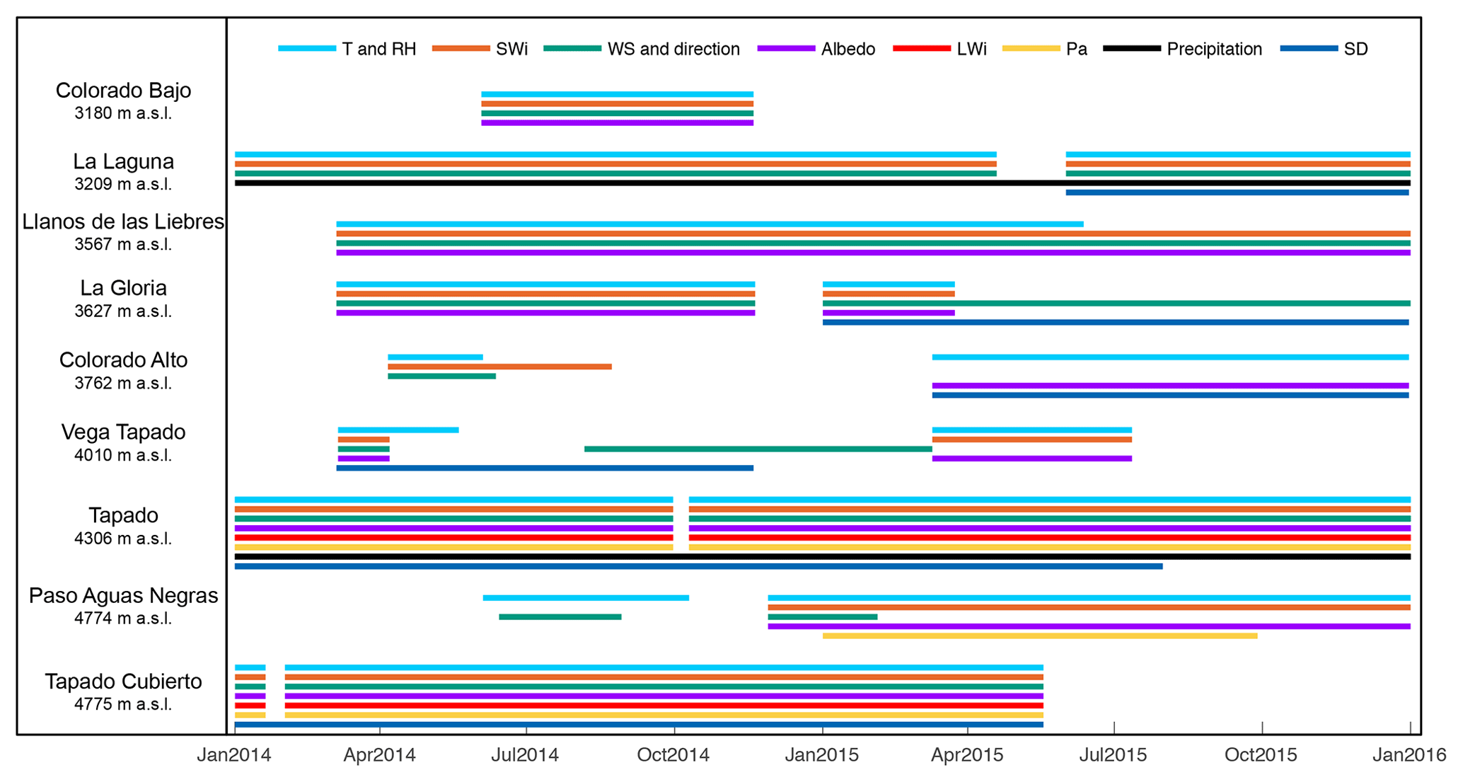
Figure 2Date of available measurements from the nine AWSs used to calibrate and validate the model. T is the air temperature, RH the relative humidity, SWi and LWi the incoming shortwave and longwave radiation, respectively, WS the wind speed, Pa the atmospheric pressure, and SD the snow depth.
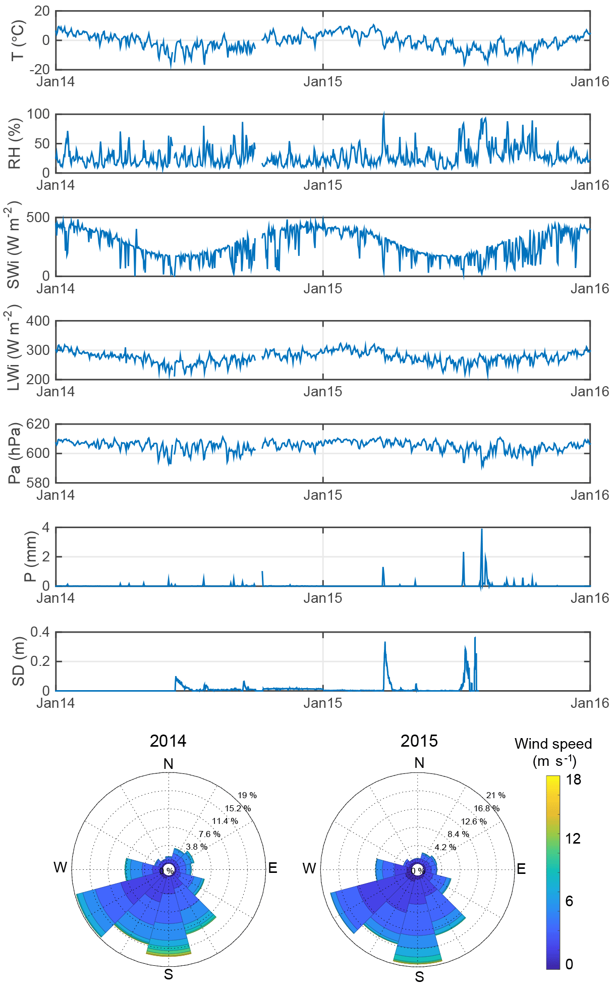
Figure 3Example of meteorological conditions of the study area. Daily air temperature (T), relative humidity (RH), incoming shortwave (SWi) and longwave (LWi) radiation, air pressure (Pa), precipitation (P), snow depth (SD), and hourly wind speed and direction (wind roses) measured at the Tapado AWS from 1 January 2014 to 31 December 2015. Note that SD measurements are available until 1 August 2015.
Due to the complexity of precipitation measurement (e.g., MacDonald and Pomeroy, 2007), datasets were post-processed. First, filters were applied to eliminate outliers (i.e., negative values and values larger than 30 mm h−1). Second, satellite images (MODIS Aqua and MODIS Terra) were used to remove recorded precipitation events on sunny days, which were probably due to wind transport. These precipitation events were only removed if five cloud-free images were available (i.e., the two for the day: one the afternoon before and one the next morning). In total, three precipitation events lower than 2 mm w.e. were removed with this method.
At Tapado, measurements are recorded at two Geonor weighing precipitation gauges, of which one is shielded (alter shield) and one is unshielded. After being filtered, the cumulative difference at the two gauges was 9.1 mm for 2014 (i.e., 10 %; 97.1 mm for unshielded gauge 1 and 106.2 mm for shielded gauge 2) and 5.4 mm for 2015 (i.e., 1 %; 457.5 mm for gauge 1 and 462.9 mm for gauge 2) with a maximum hourly difference of 1.1 mm; however the relative bias between the sensors is neither constant nor unidirectional. As the difference between the two sensors was relatively small, the mean of the two datasets was used as the reference precipitation value, and a maximum uncertainty of 10 % was estimated.
(b) WRF model outputs
The Weather Research and Forecasting (WRF) model was used to force SnowModel. WRF is usually used to predict weather for atmospheric research and operational weather forecasting. Using reanalysis data as boundary conditions, this model is able to provide hourly meteorological data such as air temperature, relative humidity, incoming radiation, wind speed and direction, atmospheric pressure, and precipitation. In this study WRF was forced by 6-hourly data from the National Centers for Environmental Prediction (NCEP) reanalysis data, at 1∘ grid resolution (Kalnay et al., 1996), as well as daily surface temperature of the ocean at 0.083∘ of resolution. The WRF model has been run using the model version 3.7.1 (Skamarock and Klemp, 2008), with default parameterizations (this choice is discussed in Sect. 5.1). The model has been run over a time period covering the entire study period (from April 2013 to April 2016). The model outputs are at 2 m above the surface (note that wind output was logarithmically scaled from 10 to 2 m height) and are available at 22 km resolution over Chile, 7 km resolution at the regional scale and 3 km resolution over the La Laguna catchment (Fig. 1). The hourly 3 km outputs (air temperature, T; relative humidity, RH; wind speed, WS, and wind direction; precipitation, P, shortwave radiation, SW; longwave radiation, LW; atmospheric pressure, Pa) over the catchment represent the virtual stations that have been used in this study.
2.2.3 Local snow depth data
In 2014, three AWSs provided snow depth measurements at an hourly time step (Vega Tapado, Tapado and Tapado Cubierto; Fig. 2). Over the 2015 winter, snow depth measurements were available at five stations (La Gloria, Colorado Alto, Tapado, La Laguna and Tapado Cubierto). The snow depths were measured with ultrasonic sensors and require post-treatment because they are particularly prone to measurement errors and typically produce a noisy signal (Lehning et al., 2002). Therefore, the control procedure described in Lehning et al. (2002) was applied to clean the signal and in particular to eliminate spikes, check for outliers and physical limits.
2.2.4 MODIS snow products
MOD10A2 (Terra) and MYD10A2 (Aqua) snow products version 5 were downloaded from the National Snow and Ice Data Center (Hall et al., 2006; Hall and Riggs, 2007) for the period 1 January 2014–1 January 2016. The binary snow products were projected on a 500 m resolution grid in the same coordinate system as the DEM. Missing values, mainly due to cloud obstruction, were interpolated using the algorithm of Gascoin et al. (2015).
3.1 SnowModel description
The physically based model SnowModel (Liston and Elder, 2006b) was used to simulate the snow depth evolution over the entire catchment. SnowModel has already shown acceptable performance in the challenging context of semiarid mountains, including the Andes (Gascoin et al. 2013, Mernild et al. 2017) and the High Atlas (Baba et al., 2018a, b) mountains. It is a spatially distributed snowpack evolution modeling system composed of four submodels briefly described below.
MicroMet is a physically based meteorological distribution model developed specifically to produce high-resolution, spatially distributed atmospheric forcing data. This model requires precipitation, wind speed and direction, temperature, and humidity as input data, generally measured at weather stations. For the incoming solar and longwave radiation and surface pressure, MicroMet can either compute these fields from other meteorological variables or create them from observations through a data assimilation procedure (Liston and Elder, 2006a). MicroMet includes a preprocessor component that first analyzes meteorological data to identify and correct potential deficiencies (e.g., values out of the ranges given in the subroutine). It then fills in any missing data segments with realistic values. The atmospheric fields are distributed using a combination of lapse rates and spatial interpolation using the Barnes objective analysis scheme (Barnes, 1964).
EnBal performs standard surface energy balance calculations (Liston, 1995; Liston et al., 1999). This component simulates surface temperatures and energy fluxes in response to observed or modeled near-surface atmospheric conditions provided by MicroMet. Surface latent and sensible heat flux and snowmelt calculations are made using a surface energy balance model.
SnowPack is a single or multilayer (max. six layers), snowpack evolution and runoff or retention model that describes snowpack changes in response to precipitation and melt fluxes defined by MicroMet and EnBal (Liston and Hall, 1995; Liston and Elder, 2006b).
SnowTrans-3D (Liston and Sturm, 1998; Liston et al., 2007) is a three-dimensional model that simulates snow depth evolution (deposition and erosion) resulting from windblown snow based on a mass balance equation that describes the temporal variation in snow depth at each grid cell within the simulation domain.
3.2 Model setup
3.2.1 Spatialized meteorological forcing
Spatial interpolation using the Barnes scheme was used to distribute the nine AWS measurements of T, RH, LWi, SWi and pressure over the model domain. As relative humidity is a nonlinear function of elevation, the relatively linear dew point temperature is used for the elevation adjustment. For more details refer to Liston and Elder (2006a). In this study the MicroMet subroutine has been run with the default setting for the Southern Hemisphere, for air temperature and dew point temperature monthly lapse rates (Liston and Elder, 2006b). Monthly lapse rates computed from the available measurements are dependent on the year considered. As the mean is close to the default settings, it has been chosen to conserve these values. Radiation values for LWi and SWi are assimilated and specified using the default parameterization (Liston and Elder, 2006a). The model has been run on the SRTM DEM and as a result, hourly meteorological data over a 100 m grid resolution are available for the entire study period. Precipitation was interpolated similarly but without considering a lapse rate, as the comparison between the available measurements did not reveal consistent elevation gradients. Wind data and direction were first interpolated using linear lapse rates and then each gridded value was corrected considering topographic slope and curvature relationships (Liston and Elder, 2006b).
The 3 km WRF outputs (Sect. 2.2.1) were used as inputs for MicroMet, which considers that each WRF cell corresponds to a virtual weather station located in the center of the WRF cell, following Mernild et al. (2017) and Baba et al. (2018a). MicroMet adjusts the elevation bias to the DEM at the corresponding coordinate and downscales the data to a 100 m grid.
3.2.2 Albedo calibration
The snow albedo evolution is computed as a function of the snow density and air temperature (more details in Liston and Hall, 1995; Liston and Elder, 2006b). Minimum and maximum values have been adjusted based on measurements. The minimum snow albedo (i.e., the soil) is fixed at 0.2 and is quite homogeneous in this basin, as there is almost no vegetation. The minimum and maximum snow albedo (corresponding to old and fresh snow, respectively) are respectively fixed to 0.6 and 0.9 in agreement with all the measurements performed at the AWSs (Fig. 2).
3.2.3 Turbulent flux calibration
As the model is using a bulk approach to simulate the turbulent fluxes, the turbulent latent and sensible heat fluxes (respectively LE and H) are parameterized using an effective surface roughness length z0 (Liston, 1995; Liston et al., 1999). Note that this roughness length z0 is considered an effective value used in the model to represent the aerodynamic (zm), temperature (zt) and humidity (zq) roughness values. As no measurements from the study period are available to calibrate and validate this value, it was initially fixed at 1 mm (Gromke et al., 2011; MacDonell et al., 2013a), and a subsequent sensitivity test was undertaken. Note that the surface temperature is solved iteratively by closing the energy balance (Liston and Elder, 2006b). In addition, under stable atmospheric conditions, turbulent fluxes are modified based on a Richardson number correction (Liston and Hall, 1995).
3.2.4 Wind transport parameterization
The model considers the wind transport (saltation, turbulent suspension) after snow deposition, sublimation of blowing and drifting snow, and erosion and deposition after snowfall, depending on the topography (Liston and Sturm, 1998). The topographic influence on wind transport has been set, following Gascoin et al. (2013). The curvature allows consideration of the typical redistribution length scale. Based on the DEM, it was estimated to be 500 m, i.e., approximately one-half the wavelength of the topographic features within the domain (Liston et al., 2007). The model considers different weights for slope and curvature values. We have chosen 0.58 and 0.42, respectively, following Gascoin et al. (2013).
3.3 Simulations
Two types of simulations have been performed over the entire catchment for the period 1 January 2014–1 January 2016 on a 100 m resolution DEM. The first simulation was forced with input from the nine automatic weather station measurements (referred to as AWS forcing), whereas the second simulation was forced with the WRF data (referred to as WRF forcing).
After indicating the differences observed for these two forcing sets, the model is primarily validated at local points. Results for the two simulations were first compared to local snow depth measurements at each AWS (described in Sect. 2.2.1). The performance was evaluated using a kappa statistic coefficient (Cohen, 1960) denoted k to measure the agreement between the simulation and the observation, considering the percentage of time with and without snow. The calculation of k is here performed according to the following formula:
where Pr(a) represents the actual observed agreement (i.e., snow or no snow for both simulation and observation), and Pr(e) represents the hypothetical probability of chance agreement. Complete agreement is defined when k=1. The root-mean-square error (RMSE) was also calculated.
Second, the model performance was evaluated over the entire catchment, by comparing the simulated snow cover extent and duration to that observed by the satellite images (described in Sect. 2.2.2). The model performance was evaluated by computing the Nash–Sutcliffe efficiency coefficient (NSE; Nash and Sutcliffe, 1970) between simulations and observations and the RMSE.
After validating the model, the sublimation ratio and sublimation and melt rates were computed over the catchment for the two years. The sublimation rate corresponds to the mass sublimated per unit of time and does not include evaporation from meltwater. The sublimation ratio is defined as a percentage and equal to the sublimation divided by the total ablation (i.e., sublimation plus melt rates). The melt rate corresponds to meltwater that runs off from the snowpack. Whilst the model calculates refreezing, the final melt rate described here does not include snowmelt that refreezes in the snowpack. Note that ablation and energy balance terms are only computed over snow surfaces. This means that annual and monthly means are only computed at grid cells with snow.
3.4 Comparison with MODIS
The snow cover area (SCA) and the snow cover duration (SCD) over the entire catchment were compared to the MODIS product. A threshold of 0.003 m w.e. was used to convert the simulated snow water equivalent (SWE) into snow presence or absence for each grid cell (within the same range as Gascoin et al., 2015). Since the MODIS SCA product corresponds to the maximum visible extent over a period of 8 d, we also computed the maximum SCA over the same 8 d period from the simulated SCA for comparison.

Figure 4(a) Area–elevation distribution of the La Laguna catchment. (b–g) MicroMet outputs at the catchment scale forced by the AWS (red) and the WRF (blue) for 2014 (lines) and 2015 (dashed lines).
4.1 Meteorological forcing comparison
4.1.1 AWS 2014 vs. 2015
According to the AWS measurements, January–July 2015 was warmer than January–July 2014. Conversely, observations indicate lower temperatures for August–December 2015 than for August–December 2014 (daily mean difference of −2.6 ∘C). Relative humidity was higher for 2015 compared to 2014 (daily mean difference of 11 %) whereas SWi was lower (mean difference of −18 W m−2, i.e., 6 % of the mean SWi), with larger differences in July–December (daily mean difference of −32 W m−2, i.e., 12 % of the daily mean SWi), and LWi was higher (daily mean difference of 20 W m−2, i.e., 7 % of the daily mean LWi). This decrease in SWi and increase in LWi can be explained by a higher degree of cloud cover in 2015.
4.1.2 MicroMet output comparison: AWS vs. WRF
Figure 4 shows MicroMet outputs forced by WRF and AWS. Colder air temperatures are observed for the WRF forcing (4.5 to 7.5 ∘C depending on the year and the elevation), as well as lower RH (between 13 % and 24 %) and higher precipitation (annual cumulative difference larger than 1 m w.e. and a difference ranging between a factor of 1.6 and 3.4 depending on the elevation; Fig. 4d). The SWi and LWi remain very similar. The wind speed outputs differ (Fig. 4e), especially above 4500 m a.s.l. where differences reach a maximum of 4 m s−1. Details and statistical information about the comparison at each AWS location are available in Table S1 (in the Supplement). Note that here the comparison between the AWS measurements and the closest WRF grid point is not presented due to the significant vertical offset between the two points (Table S1). Despite these differences between AWS and WRF, both forcings were used as inputs in order to quantify the impact of the forcing choice on the sublimation estimation in this study.
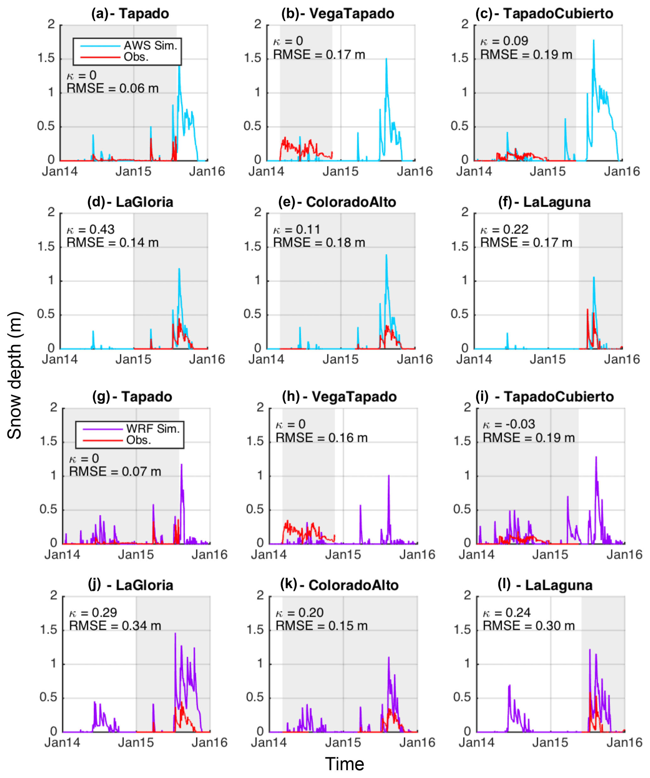
Figure 5Simulated (cyan and purple) vs. observed (red) snow depth at six automatic weather stations. Cyan lines (a–f) represent simulations performed using AWS meteorological forcing. Purple lines (g–m) correspond to simulations performed using WRF meteorological forcing. Grey shaded areas indicate the period of available measurements.
4.2 Snow depth and snow cover comparison
4.2.1 Comparison with local snow depth measurements
Simulated snow depths using the AWS forcing (Fig. 5a–f) are in good agreement with measured snow depth values (mean k=0.14 and mean RMSE =0.15 m, corresponding to 36 % of the maximum mean snow depth). Note that the largest RMSE corresponds to 63 % of the maximum snow depth. Comparisons have been performed at individual stations for 2014 and 2015, and we observe better performances across all stations (i.e., higher k and lower RMSE) for 2015 (Fig. 5d–f) than for 2014 (Fig. 5a–c). For 2014 the highest k and lower RMSEs are observed at Tapado AWS, as precipitation measurements were available at this site, but performances are much lower at the two other sites where precipitation was interpolated. Interpolation results in overestimation of the simulated snow depth during 2015, probably due to an overestimation of the precipitation for the large event on 21 June 2015 (Fig. 3) caused by large differences in measured precipitation at the La Laguna and Tapado AWSs in particular. Nevertheless, the start and the end dates of the snow season are in good agreement with observations (maximum difference of 3 d observed at La Gloria site). Note that this comparison probably overestimates the accuracy as snow depths are compared at the exact location of meteorological forcing. Larger uncertainties are expected at the interpolated locations.
Simulations performed with the WRF forcing indicate lower performances in simulating snow depth evolution at the AWS (Fig. 5g–m; mean k=0.12, and mean RMSE =0.20 m, corresponding to 39 % of the maximum mean snow depth, and the largest RMSE corresponds to 76 % of the maximum snow depth). The results indicate an overestimation of the simulated snow depth compared to the observations. In addition, for 2014, the timing of the start and the end of the snow season does not fit well with observations (and explain the low k values). In 2015, the first day of snow is generally in good agreement with observations (maximum difference of 5 d observed at La Laguna).
While AWS forcing yields a better performance overall, in both cases better correspondence is obtained for 2015. This could possibly be explained by the dry conditions in 2014, which would have resulted in precipitation having a higher spatial variability. The low snow amounts in 2014 created localized snow patches, which are complex to represent in models.
These results underline the complexity of modeling the spatial variability of snow depth (SD), even when snow transport is implemented. Results show an overall similarity of the simulated SD between some stations (e.g., Vega Tapado, Colorado Alto and La Gloria), while measurements indicate that SD is much more variable in reality. Note that the windy conditions on the local depression at Vega Tapado are very local (i.e., few meters) and make the simulation at this site where the measured SD is larger than the surrounded area and not representative of the 100 m grid cell complicated.
4.2.2 Snow cover comparison with satellite images
4.2.3 (a) Snow cover area
The simulated snow cover area (SCA), forced by the AWS forcing, is in good agreement with observations from MODIS products (Fig. 6a) with, in particular, a good simulation of the timing of precipitation events. Best fits are observed for the winter and spring 2015 (i.e., from July to December), with higher calculated correlations (NSESCA=0.94, RMSESCA=41.6 km2, i.e., 8.3 %). Regarding the ablation, in June 2014 and April–May 2015, the simulated SCA decreases faster than the observed SCA, which can be due to an overestimation of melt and/or sublimation or an underestimation of accumulation.
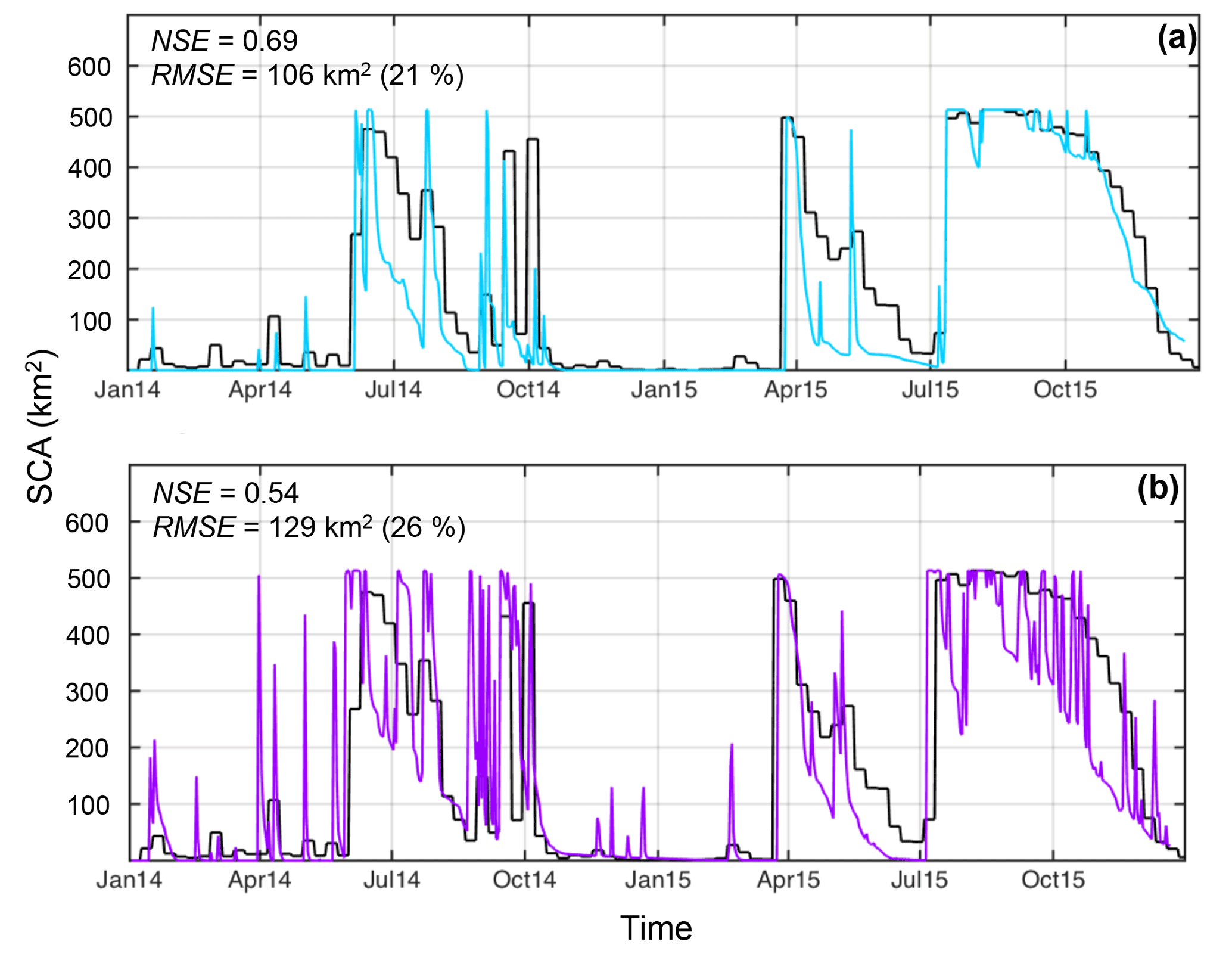
Figure 6Snow cover area evolutions over the 2014–2015 period, from MODIS images (black lines), and simulations using (a) AWS forcing (blue line) and (b) WRF forcing (purple line).
When using the WRF forcing, the agreement between SCA and MODIS is lower than with the AWS forcing (Fig. 6b). The timing of snowfall events is not always in good agreement with the observations due to missing events (e.g., March 2015), a timing bias of a few days (e.g., March 2014) and/or additional events (during both 2014 and 2015 winter). The simulated SCA evolution over winter and spring of 2015 shows strong variation over the entire catchment, which is not observed in the MODIS record. Here again, for both forcing datasets, better performances are observed for 2015 (NSEAWS=0.79, RMSEAWS=93.2 km2, i.e., 19 % of the total area; NSEWRF=0.61, RMSEWRF=125 km2 (25 %)) than for 2014 (NSEAWS=0.41, RMSEAWS=117 km2 (23 %); NSEWRF=0.23, RMSEWRF=133 km2 (27 %)).
(b) Snow cover duration over the catchment
The simulated snow cover duration (SCD) was also compared to the observed duration (from MODIS) by elevation band (Figs. 7, S2). For each 200 m elevation band, the total number of snow-covered days for each grid cell was computed and then averaged for each band. For 2014, better performances were obtained for the AWS forcing than for the WRF forcing (Fig. 7). For 2015, while better performances were also obtained for the AWS forcing, the improvement using this forcing was minor.
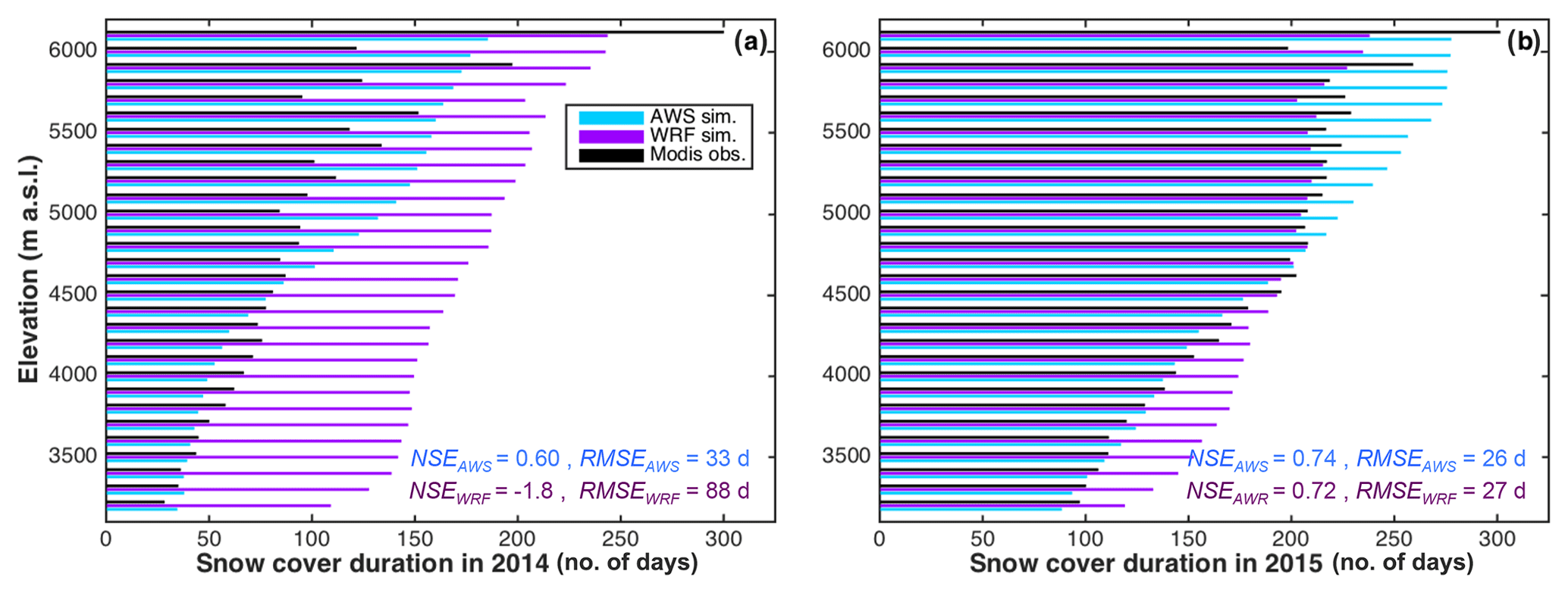
Figure 7Snow cover duration per 200 m elevation band, from MODIS images (black), AWS forcing (blue) and WRF forcing (purple) for (a) 2014 and (b) 2015.
Results based on AWS forcing are in good agreement with observations at low elevations (i.e., below 4600 m a.s.l.; Fig. 7) but show an overestimation of the SCD at high elevation (absolute mean difference of 30 and 27 d for 2014 and 2015, respectively).
When using WRF forcing, SCD is overestimated for the entire catchment in 2014 (absolute mean difference of 67 d). In 2015, simulations indicate an overestimation of the SCD at low elevations (i.e., below 4500 m a.s.l.) and a small underestimation at higher elevations (absolute mean error of 34 d for 2015).
4.3 Ablation and energy balance fluxes
The forcing strongly impacts the simulated sublimation ratio. The annual means computed over the entire catchment (only considering snow grid-cells) for the AWS forcing were 42 % and 49 % for 2014 and 2015, respectively, whereas 86 % and 80 % were obtained for WRF forcing. The mean daily rate is 0.6 and 3.6 w.e. d−1 for 2014 and 2015, respectively, when the model is forced with the AWS forcing. Values are larger and reach 3.1 mm w.e. d−1 and 4.1 mm w.e. d−1 for 2014 and 2015 when simulations are performed with the WRF forcing.
4.3.1 Mean annual elevation gradients
(a) Ablation
The annual sublimation ratio is variable in space and increases with elevation for both years and both forcings (Fig. 8a, b). Comparison between the two forcings shows larger discrepancies below 5300 m a.s.l. (50 % of differences for 2014 and 30 % for 2015). Note that larger differences were observed for 2014 related to larger differences in snow cover and snow duration between forcings.
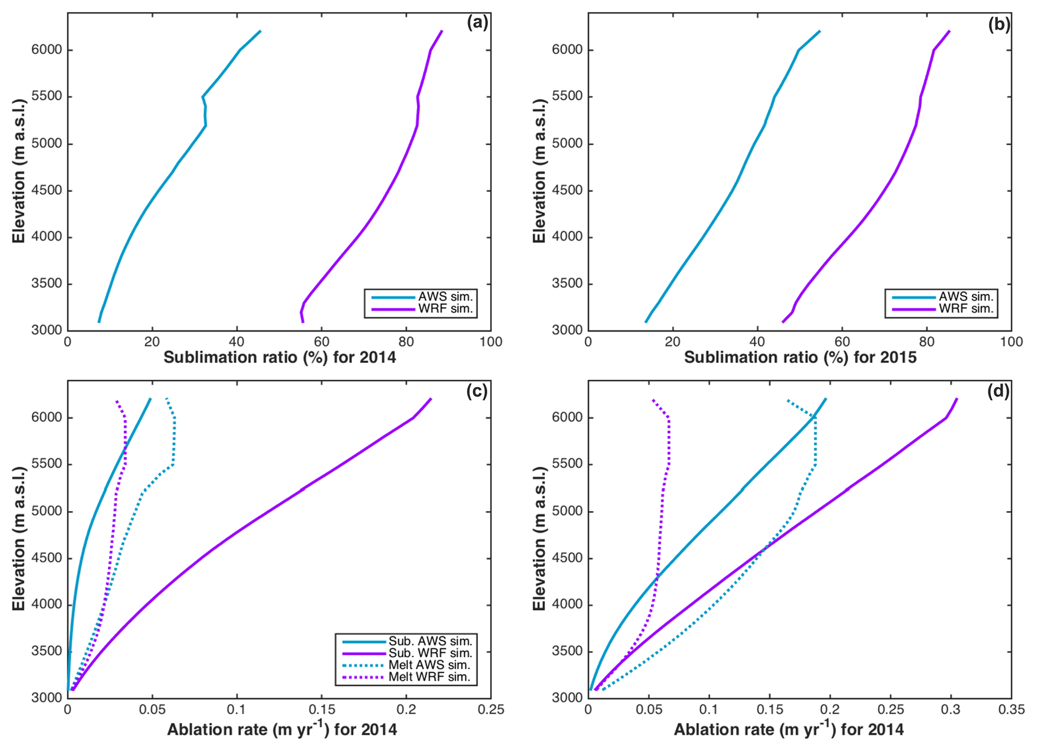
Figure 8Simulated annual sublimation ratio against elevation band using AWS (blue) and WRF (purple) forcing for 2014 (a) and 2015 (b). Simulated annual average total ablation (sublimation and melt) against the elevation using AWS and WRF forcing for 2014 (c) and 2015 (d).
Melt predominates at all elevations when using the AWS forcing (Fig. 8c, d), except above 6000 m a.s.l. in 2015. Melt and sublimation rates increase with elevation until 5300 m a.s.l. Above this elevation the melt rate first stagnates and subsequently decreases. This increase in sublimation rate and decrease in melt at high elevations explains the increase in sublimation ratio with elevation observed in Fig. 8a, b.
For the WRF forcing, sublimation rates are larger than the melt rates at all elevations. Melt is relatively constant above 3800 m a.s.l., whereas the sublimation ratio increases, explaining the larger values of the sublimation ratio at high elevations.
(b) Energy fluxes
Figure 9 shows the distribution of energy fluxes with elevation to aid the interpretation of the relationship between elevation and sublimation for both forcings. Both LW and SW show little variability between elevation bands for the AWS forcing. LW also does not change strongly between years. The SW and turbulent fluxes, however, show a strong variability between 2014 and 2015. For 2015 the modeled turbulent fluxes (mainly the latent heat flux, QE) are higher, especially at lower elevations, resulting in higher sublimation ratios (Fig. 8a, b., Sect. 4.3.1a). The WRF simulations, on the other hand, do not show this interannual difference in energy fluxes. Comparison of the AWS and WRF simulations, however, show higher turbulent fluxes for WRF forcing, which is in agreement with the higher sublimation rate and ratio mentioned above.
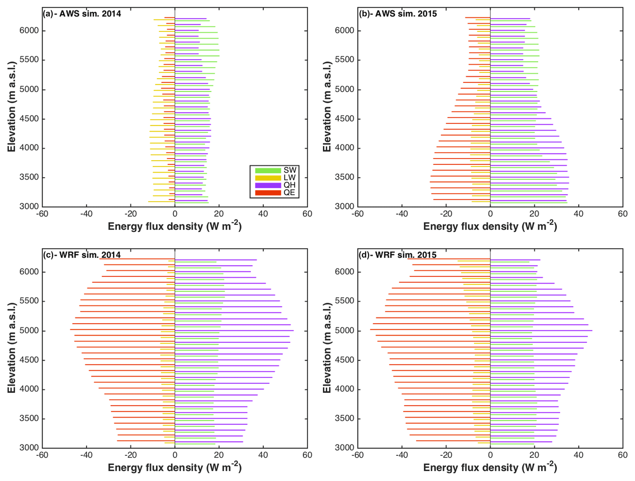
Figure 9Annual mean of main modeled energy fluxes (computed over snow surfaces only) for each 200 m elevation band using AWS (a, b) and WRF (c, d) forcing for 2014 (a, c) and 2015 (b, d). SW is net shortwave radiation, LW is net longwave radiation, QE is the latent heat flux and QH is the sensible heat flux.
4.3.2 Monthly evolution
Analysis of the monthly sublimation ratios and rate shows a strong seasonal variability in sublimation (Fig. 10). Independently of the forcing chosen, larger sublimation rates are found in June and September for 2014 and in August, September and October for 2015, corresponding to the warm parts of the snow season.
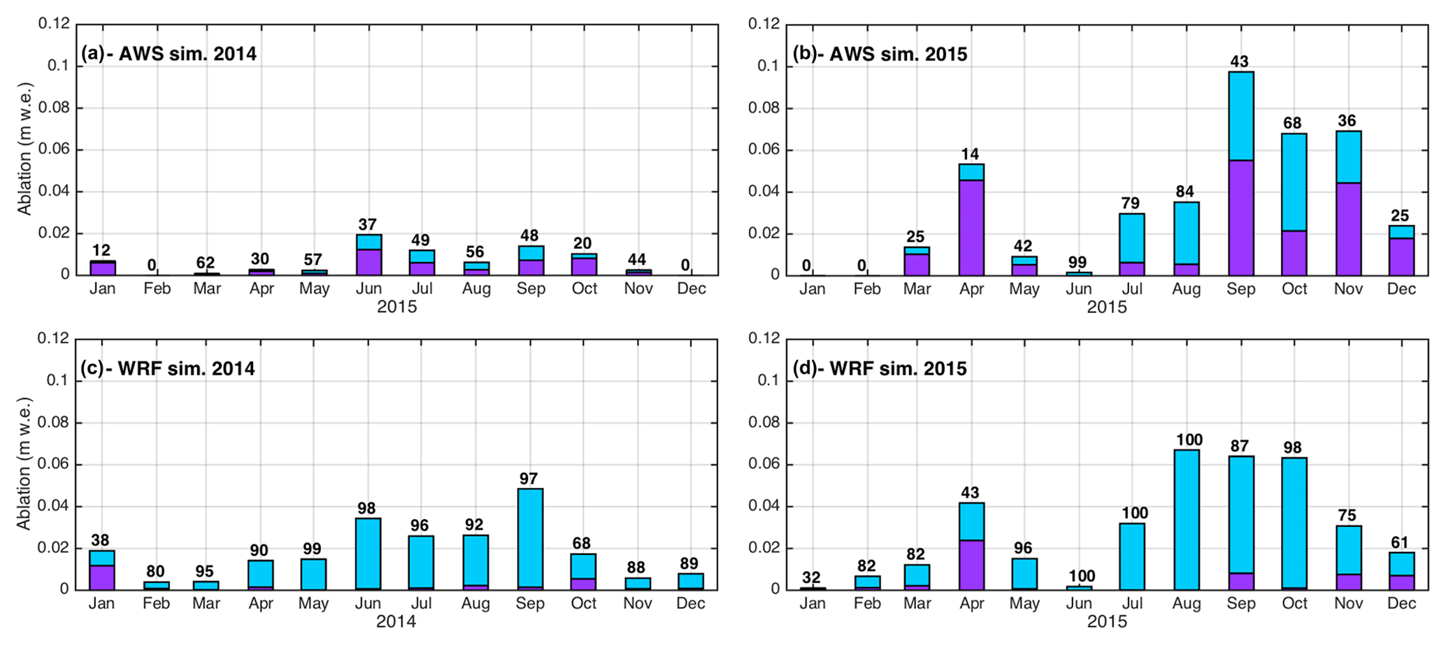
Figure 10Stacked simulated melt (purple) and sublimation (blue) per month using AWS forcing (a, b) and WRF forcing (c, d). Black numbers indicate the monthly sublimation ratio in percent.
Figure 11 indicates that turbulent fluxes (QE and QH) have the greatest impact on sublimation in all cases, except for the 2014 AWS simulation. Net SW is also an important factor, and relatively similar for all the simulations. For the annual mean, net SW is 18 and 22 W m−2 for 2014 and 2015 for the AWS forcing and 24 and 23 W m−2 for the WRF forcing, respectively. The contribution of net LW on the other hand is low for all simulations (annual mean of −7 and −6 W m−2 for AWS and WRF simulations, respectively). Note that these losses are small in comparison to midlatitude sites (e.g., −25 to −20 W m−2 according to the study by Giesen et al., 2009) because of the very dry conditions of the atmosphere and the cold surface temperature of the snow surfaces.
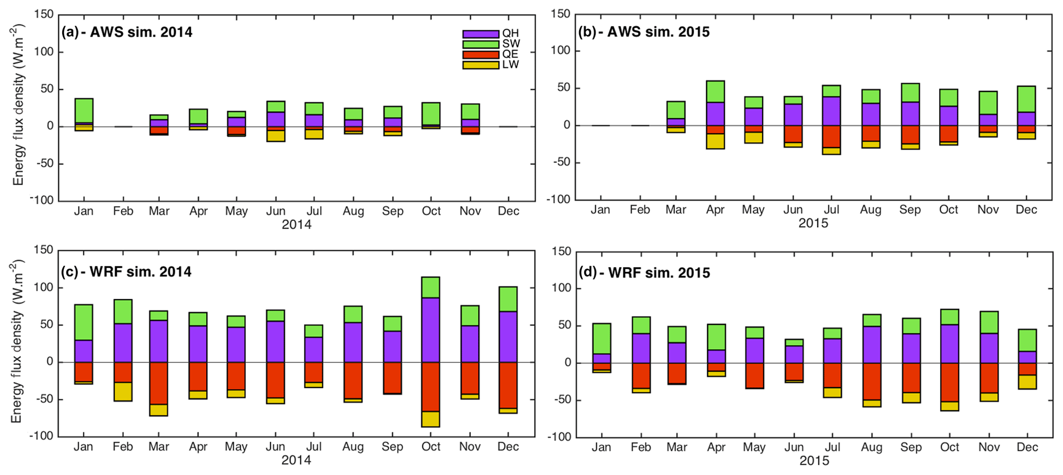
Figure 11Monthly average of the main modeled energy fluxes for the entire catchment, over snow surfaces only. SW is net shortwave radiation, LW is net longwave radiation, QE is the latent heat flux and QH is the sensible heat flux.
5.1 AWS vs. WRF forcing
Results presented in this study highlight the importance of forcing when modeling snow depth, snow cover and sublimation. Differences in model outputs are largely due to differences in temperature and precipitation inputs.
5.1.1 Air temperature and precipitation
The cold bias in air temperature from WRF simulations, using the combination NCEP–WRF, is often observed and well documented (e.g., Ruiz et al., 2010). It can be explained by the model parameterization complexity such as (i) the initial or lateral conditions, especially for the land surface surface temperature (Cheng and Steenburgh, 2005) or soil thermal conductivity (Massey et al., 2014); (ii) the parameterization of the planetary boundary layer scheme (Reeves et al., 2011); or (iii) the radiation parameterization scheme as it has been observed for other models (e.g., Müller and Scherer, 2005). However, the exact source of this bias remains difficult to identify (e.g., Reeve et al., 2011). In this study, the default parameterization has been used, but works are in progress regarding the evaluation of the most appropriate calibration over this area, using direct observations.
Otherwise, precipitation is known to be overestimated using the WRF model, particularly in the Andes (e.g., Mourre et al., 2016). One possible explanation is that biases can exist in the reanalysis data, in particular at high elevations, where observations are often scarce. Precipitation overestimation might also be related to the parameterization used for the model, which may not be the most appropriate for the Andes; further work is needed to determine the most appropriate ones. Outputs may also be inaccurate due to the relatively low-resolution DEM used (100 m).
Precipitation measurements using rain gauges can be biased towards an underestimation due to an undercatch, especially for snowfall because of the influence of wind (e.g., MacDonald and Pomeroy, 2007; Wolff et al., 2015). This gauge undercatch uncertainty (see Sect. 5.4.1) could increase the difference between the precipitation simulated by WRF and that measured at the AWSs. In addition, questions arise regarding the representativity of point measurements compared to the grid cell considered in the model.
The spatiotemporal variability observed in the difference between AWS and WRF precipitation data highlights that it would be inappropriate to use a constant correction factor to adjust WRF data with measurements. More studies comparing WRF output to AWS among other datasets are required to determine a realistic correction method.
5.1.2 Consequences of the forcing used
Biases between the two forcing datasets cause significant differences in the energy and associated mass balances during both study years. In 2014 there are lower RH and P biases (Fig. 4c, d), but larger air T differences, especially at high elevations (Fig. 4b). Wind speed is on average higher in the WRF forcing, whereas biases in incoming LW and SWi and air pressure are low for both years (results not shown).
The larger RH bias in 2015 indicates an overestimation of the dryness for this year (compared to 2014) and would lead to larger differences in sublimation rate for 2015 than for 2014, which is the opposite of the results observed. Likewise, the larger overestimation of precipitation amount observed in 2015 (Fig. 4d) does not explain the larger difference in sublimation, as a deeper snow depth should result in more persistent snow cover during the warm period and hence a lower sublimation ratio related to larger melt rate. Therefore, although the relationship between temperature and sublimation rate is complex and not necessarily direct, in this case, the colder temperature is the most probable explanation for at least part of the larger difference in sublimation rate observed at high elevation.
Lower temperature and relative humidity values from WRF outputs compared to AWS measurements can explain, in part, the larger simulated sublimation ratio found with this forcing (Figs. 8a, b and 10). The relatively high amounts of precipitation simulated by the WRF outputs, and resulting snow cover overestimation, may also play a role. Differences in the sublimation ratio when using the AWS and WRF forcing are quite similar for the two years (mean annual difference of 42 % and 36 % for 2014 and 2015, respectively), although the difference between the melt rate and sublimation rate depends on the year (Figs. 8c, d) and corresponding energy balance.
In 2014 the turbulent fluxes are dominant for the WRF forcing but not for the AWS forcing (Fig. 9a, c). This can be partially explained by the larger SCA simulated by WRF forcing with snow cover in the entire catchment while the AWS forcing only results in snow at higher elevations. Additionally, WRF forcing indicates colder, drier and windier conditions than the AWS forcing (Fig. 4). Lower RH and higher wind speed will directly increase the latent heat flux, and potentially sublimation ratio, depending on surface temperature (see Fig. S3 for surface temperature comparison).
The large variation in the SCA resulting from the WRF-driven model results (Fig. 5) is likely related to the higher frequency of relatively small precipitation events modeled by WRF than are recorded by the AWS. These small events cover the catchment with a relatively thin layer of fresh snow, which sublimates relatively quickly, causing the SWE to decrease to < 3 mm w.e. at lower elevations, causing high variability in modeled SCA.
The SCD also has a significant influence on sublimation. For 2014, the differences in SCD between the two forcings were 100 d below 4500 m and close to 50 d above this elevation (Fig. 7a). Snow that persists until later in the year (austral spring and summer) results in an increased total melt rate and can influence the sublimation ratio (especially in 2015, Fig. 10). This is the only explanation for the larger melt fraction observed with AWS forcing compared to WRF forcing at low elevations, given the cold bias in WRF forcing (Figs. 8c and 4b). Since a larger SCD can be related to larger precipitation amount, precipitation uncertainties likely play a significant role in the sublimation estimation.
5.2 Comparison between dry and wet conditions
5.2.1 Comparison between 2014 and 2015
Differences in sublimation ratio and rates between 2014 and 2015 are related to both meteorological conditions related to energy fluxes and snow cover duration. First, the similar annual mean sublimation ratio found for both years is likely due to a compensation between the dry 2014 year (low precipitation) associated with cold conditions in spring and summer and the wet 2015 year with longer snow duration and warmer spring and summer (according to meteorological measurements made in the region). Both sublimation and melt rates were larger overall during the wet 2015 year compared to the dry 2014 year. Thus the higher melting rates in 2015 compensated for the enhanced sublimation rates and resulted in sublimation ratios comparable with 2014. The larger sublimation rates observed in 2015 are related to higher RH and wind speed, but also higher precipitation, snow accumulation and snow duration in 2015 compared to 2014. Results show particularly large sublimation rates over the long melt period in 2015. This may be explained by the warmer conditions which induce a warmer snowpack, increasing the saturated vapor pressure at the snow surface and providing energy to increase the sublimation rates (Herrero and Polo, 2016). According to these results, the snow duration seems to modulate the annual average ablation ratio, such that a longer-lasting snow cover extending further into the warm spring climate is subjected to both enhanced sublimation and melt in response to an increase in incoming energy fluxes. Nevertheless, it remains difficult to disentangle the respective effects of meteorological conditions and snow duration on sublimation. To better evaluate these effects, the influence of the meteorological forcing related to energy fluxes and the snow cover duration must be evaluated separately. For that purpose, we performed simulation experiments in which a common precipitation input was used for both years. In the first experiment the 2014 precipitation inputs (“dry input” with shorter snow cover duration) were applied to both years, and then the 2015 precipitation was applied to both years (“wet input” with longer snow cover duration). All other meteorological forcings were left unchanged.
5.2.2 Impact of the precipitation amount
Forcing the 2014 year with the wet precipitation input reduces the mean annual sublimation ratio by 12 % (Fig. 12a, d), while forcing the 2015 year with the dry precipitation input increases the mean annual sublimation ratio by 3 % (Fig. 12b, d). In summary, a decreased annual mean sublimation ratio is observed when the precipitation is increased (which likely increases the SD and SCD) and other factors are held constant. However the amplitude of the response differs between the two years. This is mainly due to differences in the ablation rates (Fig. 12). For 2014, increasing the precipitation amount leads to a sublimation rate increase of 0.8 mm w.e. d−1 while for 2015, decreasing the precipitation amount decreases the rate by 2.8 mm w.e. d−1. Despite these annual differences, the maximum monthly sublimation rates are still observed for the same months, independent of the precipitation forcing used, with the exception of June and August (Fig. 12). In June, snow covered the entire catchment in 2014 but not in 2015 (Fig. 6), related to a strong snow event in June 2014 and no precipitation in June 2015. The opposite was observed for August. Changing the precipitation forcing strongly impacts the SCA and therefore the snow amount available for ablation and sublimation.
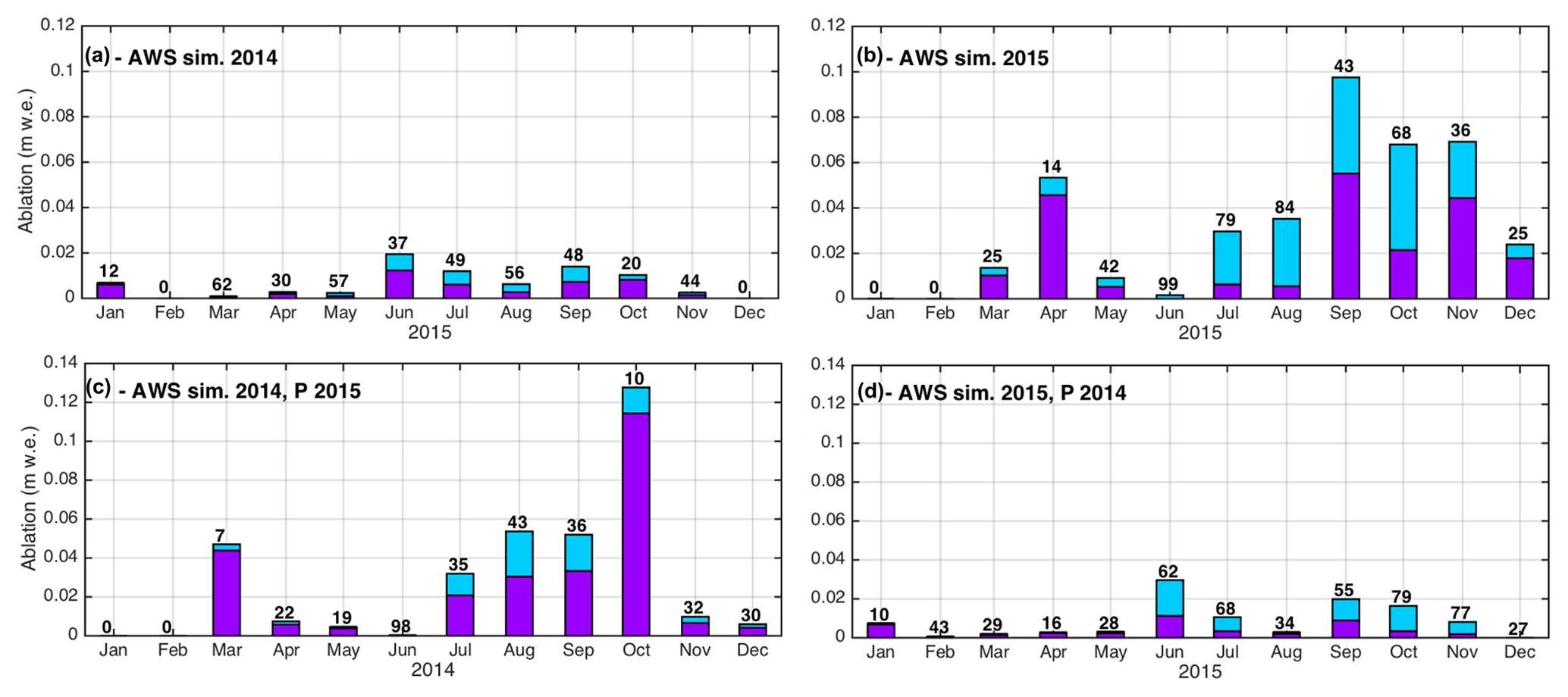
Figure 12Monthly simulated melt (purple) and sublimation (blue) using AWS forcing (a, b) and AWS forcing with (c) 2015 precipitation (“wet forcing”) and (d) 2014 precipitation (“dry forcing”). Back numbers indicate the monthly sublimation ratio in percent.
Comparisons made for months with a maximum SCA (i.e., when the entire catchment is covered by snow and it persists over the entire month) allow the influence of SCD to be independently analyzed since the SCA remains constant. In July, a month where maximum SCA was observed in both years, sublimation differences of 27 and 57 mm w.e. m−1 were found between dry and wet precipitation inputs for 2014 and 2015, respectively. In 2015 the SD was thicker than in 2014 for both dry and wet inputs; thus the results indicate an increased sublimation rate with thicker SD. The thicker SD also implies larger melt rates, such that the sublimation ratio decreases when increasing the precipitation in 2014 but increases with increased precipitation in 2015, highlighting the complexity of the influence of SD on the sublimation ratio.
Otherwise, differences in mean sublimation rates are much higher when changing the precipitation amount for the 2015 meteorological forcing than for the 2014 meteorological forcing (i.e., 0.8 mm w.e. d−1 for 2014 vs. 2.8 mm w.e. d−1 for 2015 as mentioned above). Sublimation rates are also higher in 2015 compared to 2014, especially at the end of the snow season (i.e., from September to November; Figs. 12a, d). This holds true when considering wet conditions (Fig. 12b, c). This highlights the significant influence of meteorological conditions on sublimation. As mentioned in Sect. 5.2.1, 2015 experienced higher wind speeds and RH and colder air temperatures. The contribution of turbulent fluxes is higher in 2015 than 2014 (Fig. S4a, d), suggesting that wind speed has a greater influence on sublimation than RH.
5.3 Limits of the study
The main objective of this study was to investigate the impact of forcing data on modeled mass and energy balance to explain sublimation ratios. Nevertheless, we recognize that uncertainties also exist depending on model calibration choices. To discuss this point, four different parameters were tested to evaluate the uncertainties related to the calibration of modeled parameters: roughness value, precipitation amounts (due to measurement uncertainties), topographic curvature length and slope versus curvature length (Fig. S5; Supplement Sect. S6). The results showed that the sublimation ratio was most sensitive to roughness values and that differences due to the other three variables were an order of magnitude lower (for more details, please refer to the Supplement). The strong sensitivity to the roughness value and the absence of measurements to validate the turbulent fluxes' calibration limits precise sublimation quantification for this area.
In this study, the snow energy and mass balance have been simulated over La Laguna catchment located in the semiarid Andes of Chile. Using the snowpack model SnowModel, simulations were performed over two contrasting years (2014 considered a dry year and 2015 considered a wet year), using two distinct forcings (nine AWS located in the catchment and 3 km resolution WRF model outputs).
Results indicate strong differences in simulated snow depth depending on the forcing chosen, mainly due to a cold bias in air temperature in WRF as well as an overestimation of precipitation. As a result, performances in simulating the snow cover using the AWS forcing are more realistic, both at the local scale (comparison with AWS snow depth measurements) and over the entire catchment (comparison with SCA and SCD from MODIS images). In addition, independently of the forcing choice, the simulation of snow cover is better for 2015 compared to 2014, mainly due to a larger sensitivity to the precipitation uncertainties during dry conditions. This highlights the complexity in properly modeling the snow cover evolution for years with low precipitation.
There are also large differences in modeled sublimation ratio depending on the forcing chosen. When using WRF forcing the sublimation ratio is approximately twice that modeled with the AWS forcing. This is partially due to the differences in temperature and relative humidity between the two forcings, but mostly due to precipitation differences. For example, when holding all model inputs constant except for precipitation, there are significant differences in the modeled sublimation, especially for 2014, which was a dry year. Otherwise, the annual mean of the sublimation ratio over a catchment is similar during the two years, but it increases with elevation. This partly explains the larger sublimation values reported in previous studies performed at high elevations in the semiarid Andes of Chile (e.g., Gascoin et al., 2013; Ginot et al., 2001; MacDonell et al., 2013a).
Sublimation simulated in this study is associated with several sources of uncertainty related to the forcing chosen and the model calibration. Regarding the calibration, the roughness value is the key concern to properly simulate the turbulent fluxes, and results showed strong sensitivity to this value. Nevertheless, without measurements to properly calibrate this value, it appears to be the main source of model calibration uncertainty. Results presented here highlight precipitation as the main forcing uncertainty, due to measurement errors and lack of spatial representation as precipitation data were only available for two stations. Precipitation uncertainties directly impact snow on the ground and therefore indirectly impact sublimation rates. Uncertainties in wind speed were likely the second source of error in sublimation results, which need to be better constrained in future studies. Therefore, this study highlights that this uncertainty has a strong impact on sublimation and further work is suggested to (i) improve measurement uncertainties, (ii) increase the number of sensors over the catchment, and (iii) incorporate AWS measurements into the WRF model and use data assimilation to improve model outputs. CEAZA is currently working on point (iii) to provide improved WRF outputs for the semiarid Andes of Chile. This study has highlighted the current difficulties in using standard WRF model outputs in a semiarid Andean catchment. Moving forward, it would be highly advantageous to improve WRF model performance in mountainous areas where high relief and difficult access often limit AWS distribution to valley floors, therein limiting the accuracy of interpolation techniques for terrain-sensitive variables, such as precipitation and wind speed and direction.
Part of the data used in this paper (automatic weather station data) can be accessed at https://www.ceazamet.cl (CEAZA, 2020). Satellite images are available by contacting Simon Gascoin. Data were processed using the snowpack model SnowModel and this algorithm can be accessed by contacting the administrator, Glen E. Liston. For any other access to the data presented in this study, please contact the corresponding author.
The supplement related to this article is available online at: https://doi.org/10.5194/tc-14-147-2020-supplement.
MR and SM designed the study. MR and SG designed the modeling strategy. MR ran the numerical experiments and conducted data preparation and analyses. SG provided the MODIS data. MR, SM and CK collected and provided the field meteorological data. All authors contributed to the preparation of the paper.
The authors declare that they have no conflict of interest.
The authors thank Glen E. Liston for providing SnowModel code and for the interesting and useful discussions and suggestions. We are also grateful to Pablo Salinas and Arno Hammann for providing the WRF simulation outputs and for providing useful assistance related to these data. Finally we acknowledge Jonathan Conway and Kay Helfricht for their detailed comments and the helpful suggestions which significantly improved the quality of the paper.
Marion Réveillet and Shelley MacDonell were supported by CONICYT-Programa Regional R16A10003, and the Coquimbo regional government FIC-R(2015) BIP 30403127-0. Christophe Kinnard was supported by a Coopération bilatérale – Québec-Chili Ministère des Relations Internationales et Francophonie.
This paper was edited by Ross Brown and reviewed by Jonathan Conway and Kay Helfricht.
Ayala, A., Pellicciotti, F., MacDonell, S., McPhee, J., and Burlando, P.: Patterns of glacier ablation across North-Central Chile: Identifying the limits of empirical melt models under sublimation-favorable conditions, Water Resour. Res., 53, 5601–5625, https://doi.org/10.1002/2016WR020126, 2017.
Baba, M., Gascoin, S., and Hanich, L: Assimilation of Sentinel-2 Data into a Snowpack Model in the High Atlas of Morocco, Remote Sens., 10, 1982, https://doi.org/10.3390/rs10121982, 2018a.
Baba, M., Gascoin, S., Jarlan, L., Simonneaux, V., and Hanich, L.: Variations of the Snow Water Equivalent in the Ourika Catchment (Morocco) over 2000–2018 Using Downscaled MERRA-2 Data, Water, 10, 1120, https://doi.org/10.3390/w10091120, 2018b.
Barnes, S. L.: A technique for maximizing details in numerical weather map analysis, J. Appl. Meteorol., 3, 396–409, 1964.
Burger, F., Ayala, A., Farias, D., Shaw, T. E., MacDonell, S., Brock, B., McPhee, J., and Pellicciotti, F.: Interannual variability in glacier contribution to runoff from a high-elevation Andean catchment: understanding the role of debris cover in glacier hydrology, Hydrol. Process., 33, 214–229, https://doi.org/10.1002/hyp.13354, 2019.
CEAZA: AWS data, available at: https://www.ceazamet.cl, last access: 10 January 2020.
Cheng, W. Y. and Steenburgh, W. J.: Evaluation of surface sensible weather forecasts by the WRF and the Eta models over the western United States, Weather Forecast., 20, 812–821, 2005.
Christie, D. A., Lara, A., Barichivich, J., Villalba, R., Morales, M. S., and Cuq, E.: El Niño-Southern Oscillation signal in the world's highest-elevation tree-ring chronologies from the Altiplano, Central Andes, Palaeogeogr. Palaeocl., 281, 309–319, 2009.
Cohen, J.: A coefficient of agreement for nominal scale, Educ. Psychol. Meas., 20, 37–46, 1960.
Falvey, M. and Garreaud, R.: Wintertime Precipitation Episodes in Central Chile: Associated Meteorological Conditions and Orographic Influences, J. Hydrometeorol., 8, 171–193, https://doi.org/10.1175/JHM562.1, 2007.
Favier, V., Falvey, M., Rabatel, A., Praderio, E., and López, D.: Interpreting discrepancies between discharge and precipitation in high-altitude area of Chile's Norte Chico region (26–32∘ S), Water Resour. Res., 45, W02424, https://doi.org/10.1029/2008WR006802, 2009.
Garreaud, R. D.: The Andes climate and weather, Adv. Geosci.,22, 3–11, https://doi.org/10.5194/adgeo-22-3-2009, 2009.
Garreaud, R. D., Rutllant, J. A., Muñoz, R. C., Rahn, D. A., Ramos, M., and Figueroa, D.: VOCALS-CUpEx: the Chilean Upwelling Experiment, Atmos. Chem. Phys., 11, 2015–2029, https://doi.org/10.5194/acp-11-2015-2011, 2011.
Gascoin, S., Kinnard, C., Ponce, R., Lhermitte, S., MacDonell, S., and Rabatel, A.: Glacier contribution to streamflow in two headwaters of the Huasco River, Dry Andes of Chile, The Cryosphere, 5, 1099–1113, https://doi.org/10.5194/tc-5-1099-2011, 2011.
Gascoin, S., Lhermitte, S., Kinnard, C., Bortels, K., and Liston, G. E.: Wind effects on snow cover in Pascua-Lama, Dry Andes of Chile, Adv. Water Resour., 55, 25–39, https://doi.org/10.1016/j.advwatres.2012.11.013, 2013.
Gascoin, S., Hagolle, O., Huc, M., Jarlan, L., Dejoux, J.-F., Szczypta, C., Marti, R., and Sánchez, R.: A snow cover climatology for the Pyrenees from MODIS snow products, Hydrol. Earth Syst. Sci., 19, 2337–2351, https://doi.org/10.5194/hess-19-2337-2015, 2015.
Giesen, R. H., Andreassen, L. M., van den Broeke, M. R., and Oerlemans, J.: Comparison of the meteorology and surface energy balance at Storbreen and Midtdalsbreen, two glaciers in southern Norway, The Cryosphere, 3, 57–74, https://doi.org/10.5194/tc-3-57-2009, 2009.
Ginot, P., Kull, C., Schwikowski, M., Schotterer, U., and Gäggeler, H. W.: Effects of postdepositional processes on snow composition of a subtropical glacier (Cerro Tapado, Chilean Andes), J. Geophys. Res.-Atmos., 106, 32375–32386, 2001.
Gromke, C., Manes, C., Walter, B., Lehning, M., and Guala, M.: Aerodynamic Roughness Length of Fresh Snow, Bound.-Lay. Meteorol., 141, 21–34, https://doi.org/10.1007/s10546-011-9623-3, 2011.
Hall, D. K. and Riggs, G. A.: Accuracy assessment of the MODIS snow products, Hydrol. Process., 21, 1534–1547, https://doi.org/10.1002/hyp.6715, 2007.
Hall, D. K., Riggs, G. A., and Salomonson, V. V.: MODIS snow and sea ice products, in: Earth Science Satellite Remote Sensing, Springer, 154–181, 2006.
Herrero, J. and Polo, M. J.: Evaposublimation from the snow in the Mediterranean mountains of Sierra Nevada (Spain), The Cryosphere, 10, 2981–2998, https://doi.org/10.5194/tc-10-2981-2016, 2016.
Kalnay, E., Kanamitsu, M., Kistler, R., Collins, W., Deaven, D., Gandin, L., Iredell, M., Saha, S., White, G., and Woollen, J.: The NCEP/NCAR 40-year reanalysis project, B. Am. Meteorol. Soc., 77, 437–472, 1996.
Lehning, M., Bartelt, P., Brown, B., and Fierz, C.: A physical SNOWPACK model for the Swiss avalanche warning: Part III: Meteorological forcing, thin layer formation and evaluation, Cold Reg. Sci. Technol., 35, 169–184, 2002.
Liston, G. E.: Local Advection of Momentum, Heat, and Moisture during the Melt of Patchy Snow Covers, J. Appl. Meteorol., 34, 1705–1715, https://doi.org/10.1175/1520-0450-34.7.1705, 1995.
Liston, G. E., Bruland, O., Elvehøy, H., Sand, K.: Below-surface ice melt on the coastal Antarctic ice sheet, J. Glaciol., 45, 273–285, https://doi.org/10.3189/002214399793377130, 1999.
Liston, G. E. and Elder, K.: A Meteorological Distribution System for High-Resolution Terrestrial Modeling (MicroMet), J. Hydrometeorol., 7, 217–234, https://doi.org/10.1175/JHM486.1, 2006a.
Liston, G. E. and Elder, K.: A Distributed Snow-Evolution Modeling System (SnowModel), J. Hydrometeorol., 7, 1259–1276, https://doi.org/10.1175/JHM548.1, 2006b.
Liston, G. E. and Hall, D. K.: An energy-balance model of lake-ice evolution, J. Glaciol., 41, 373–382, 1995.
Liston, G. E. and Sturm, M.: A snow-transport model for complex terrain, J. Glaciol., 44, 498–516, 1998.
Liston, G. E., Haehnel, R. B., Sturm, M., Hiemstra, C. A., Berezovskaya, S., and Tabler, R. D.: Instruments and methods simulating complex snow distributions in windy environments using SnowTran-3D, J. Glaciol., 53, 241–256, 2007.
MacDonald, J. and Pomeroy, J. W.: Gauge undercatch of two common snowfall gauges in a prairie environment, Proceedings of the 64th Eastern Snow Conference, 119–126, 2007.
MacDonell, S., Kinnard, C., Mölg, T., Nicholson, L., and Abermann, J.: Meteorological drivers of ablation processes on a cold glacier in the semi-arid Andes of Chile, The Cryosphere, 7, 1513–1526, https://doi.org/10.5194/tc-7-1513-2013, 2013a.
MacDonell, S., Nicholson, L., and Kinnard, C.: Parameterisation of incoming longwave radiation over glacier surfaces in the semi-arid Andes of Chile, Theor. Appl. Climatol., 111, 513–528, https://doi.org/10.1007/s00704-012-0675-1, 2013b.
Massey, J. D., Steenburgh, W. J., Hoch, S. W., and Knievel, J. C.: Sensitivity of Near-Surface Temperature Forecasts to Soil Properties over a Sparsely Vegetated Dryland Region, J. Appl. Meteorol. Climatol., 53, 1976–1995, https://doi.org/10.1175/JAMC-D-13-0362.1, 2014.
Mernild, S. H., Liston, G. E., Hiemstra, C. A., Malmros, J. K., Yde, J. C., and McPhee, J.: The Andes Cordillera. Part I: snow distribution, properties, and trends (1979–2014), J. Climatol., 37, 1680–1698, https://doi.org/10.1002/joc.4804, 2017.
Montecinos, A., Díaz, A., and Aceituno, P.: Seasonal diagnostic and predictability of rainfall in subtropical South America based on tropical Pacific SST, J. Climate, 13, 746–758, 2000.
Mourre, L., Condom, T., Junquas, C., Lebel, T., E. Sicart, J., Figueroa, R., and Cochachin, A.: Spatio-temporal assessment of WRF, TRMM and in situ precipitation data in a tropical mountain environment (Cordillera Blanca, Peru), Hydrol. Earth Syst. Sci., 20, 125–141, https://doi.org/10.5194/hess-20-125-2016, 2016.
Müller, M. D. and Scherer, D.: A grid-and subgrid-scale radiation parameterization of topographic effects for mesoscale weather forecast models, Mon. Weather Rev., 133, 1431–1442, 2005.
Nash, J. E. and Sutcliffe, J. V.: River flow forecasting through conceptual models part I – A discussion of principles, J. Hydrol., 10, 282–290, https://doi.org/10.1016/0022-1694(70)90255-6, 1970.
Rabatel, A., Castebrunet, H., Favier, V., Nicholson, L., and Kinnard, C.: Glacier changes in the Pascua-Lama region, Chilean Andes (29∘ S): recent mass balance and 50 yr surface area variations, The Cryosphere, 5, 1029–1041, https://doi.org/10.5194/tc-5-1029-2011, 2011.
Reeves, H. D., Elmore, K. L., Manikin, G. S., and Stensrud, D. J.: Assessment of Forecasts during Persistent Valley Cold Pools in the Bonneville Basin by the North American Mesoscale Model, Weather Forecast., 26, 447–467, https://doi.org/10.1175/WAF-D-10-05014.1, 2011.
Ruiz, J. J., Saulo, C., and Nogués-Paegle, J.: WRF Model Sensitivity to Choice of Parameterization over South America: Validation against Surface Variables, Mon. Weather Rev., 138, 3342–3355, https://doi.org/10.1175/2010MWR3358.1, 2010.
Sinclair, K. E. and MacDonell, S.: Seasonal evolution of penitente glaciochemistry at Tapado Glacier, Northern Chile: Seasonal Evolution of Penitente Glaciochemistry, Northern Chile, Hydrol. Process., 30, 176–186, https://doi.org/10.1002/hyp.10531, 2016.
Skamarock, W. C. and Klemp, J. B.: A time-split nonhydrostatic atmospheric model for weather research and forecasting applications, J. Comput. Phys., 227, 3465–3485, 2008.
Wolff, M. A., Isaksen, K., Petersen-Øverleir, A., Ødemark, K., Reitan, T., and Brækkan, R.: Derivation of a new continuous adjustment function for correcting wind-induced loss of solid precipitation: results of a Norwegian field study, Hydrol. Earth Syst. Sci., 19, 951–967, https://doi.org/10.5194/hess-19-951-2015, 2015.