Permafrost variability over the Northern Hemisphere based on the MERRA-2 reanalysis

This study introduces and evaluates a comprehensive, model-generated dataset of Northern Hemisphere permafrost conditions at 81 km² resolution. Surface meteorological forcing fields from the Modern-Era Retrospective Analysis for Research and Applications 2 (MERRA-2) reanalysis were used to drive an improved version of the land component of MERRA-2 in middle-to-high northern latitudes from 1980 to 2017. The resulting simulated permafrost distribution across the Northern Hemisphere mostly captures the observed extent of continuous and discontinuous permafrost but misses the ecosystem-protected permafrost zones in western Siberia. Noticeable discrepancies also appear along the southern edge of the permafrost regions where sporadic and isolated permafrost types dominate. The evaluation of the simulated active layer thickness (ALT) against remote sensing retrievals and in situ measurements demonstrates reasonable skill except in Mongolia. The RMSE (bias) of climatological ALT is 1.22 m (−0.48 m) across all sites and 0.33 m (−0.04 m) without the Mongolia sites. In northern Alaska, both ALT retrievals from airborne remote sensing for 2015 and the corresponding simulated ALT exhibit limited skill versus in situ measurements at the model scale. In addition, the simulated ALT has larger spatial variability than the remotely sensed ALT, although it agrees well with the retrievals when considering measurement uncertainty. Controls on the spatial variability of ALT are examined with idealized numerical experiments focusing on northern Alaska; meteorological forcing and soil types are found to have dominant impacts on the spatial variability of ALT, with vegetation also playing a role through its modulation of snow accumulation. A correlation analysis further reveals that accumulated above-freezing air temperature and maximum snow water equivalent explain most of the year-to-year variability of ALT nearly everywhere over the model-simulated permafrost regions.

1 Introduction

Permafrost is an important component of the climate system, and its variations can have significant impacts on climate and society. Of deep concern is a potential positive feedback loop by which carbon stored within permafrost regions is released through global warming, thereby adding greenhouse gases to the atmosphere that accelerate the warming further (Dorrepaal et al., 2009; Schuur et al., 2009; MacDougall et al., 2012; Schuur et al., 2015). Communities and infrastructure in ice-rich permafrost regions are particularly vulnerable to land subsidence and infrastructure damage caused by permafrost thaw (Nelson et al., 2001; Liu et al., 2010; Guo and Sun, 2015).

Permafrost variations, including pronounced permafrost degradation due to a warming climate, have been reported for many regions, including Alaska (Nicholas and Hinkel, 1996; Osterkamp and Romanovsky, 1996; Jorgenson et al., 2001; Hinkel and Nelson, 2003; Jafarov et al., 2012; Liu et al., 2012; Jones et al., 2016; Batir et al., 2017), Canada (Chen et al., 2003; James et al., 2013), Norway (Gisnas et al., 2013), Sweden (Pannetier and Frampton, 2016), Russia (Romanovsky et al., 2007, 2010), Mongolia (Sharkhuu and Sharkhuu, 2012), and the Qinghai–Tibet Plateau (Zhou et al., 2013; Wang et al., 2016a; Lu et al., 2017; Ran et al., 2018). For the entire Northern Hemisphere, rapidly accelerated permafrost degradation in recent years has been reported by Luo et al. (2016) based on in situ measurements at a point scale or a spatially aggregated scale (up to 1000 m × 1000 m) from the Circumpolar Active Layer Monitoring (CALM) network. However, the current state and evolution of global permafrost (including permafrost temperature, ice content, and degradation rates) are still largely unknown across much of the northern latitudes.

The impact of a changing climate on permafrost dynamics must depend on local site characteristics. Subsurface heat transfer processes and active layer thickness (ALT; the maximum thaw depth at the end of the thawing season) are influenced by more than surface meteorological forcing – they are also influenced by vegetation type, surface organic layer characteristics, soil properties, and soil moisture (Stieglitz et al., 2003; Shur and Jorgenson, 2007; Yi et al., 2007, 2015; Luetschg et al., 2008; Dankers et al., 2011; Johnson et al., 2013; Jean and Payette, 2014; Fisher et al., 2016; Matyshak et al., 2017; Tao et al., 2017). Understanding the contributions from the different controls on ALT (and permafrost conditions in general) is crucial for assessing permafrost behaviour and its resilience to a warming climate.

Physically based numerical model simulations are potentially useful for quantifying and understanding these dynamics at large spatial scales; they can also provide insights into associated impacts on the global carbon cycle. Permafrost dynamics can be modelled, for example, by driving a land surface model (LSM) offline (i.e. uncoupled from an atmospheric model) with meteorological forcing data (including air temperature, radiation, and precipitation) from some credible source. LSMs that have been used to quantify large-scale permafrost patterns (i.e. distributions and thermal states) and their interactions with a warming climate include, for example, the Joint UK Land Environment Simulator (JULES, Dankers et al., 2011), the Organizing Carbon and Hydrology in Dynamic Ecosystems (ORCHIDEE) – aMeliorated Interactions between Carbon and Temperature (ORCHIDEE-MICT, Guimberteau et al., 2018), the Catchment Land Surface Model (CLSM, Tao et al., 2017), and the Community Land Model (CLM; Alexeev et al., 2007; Nicolsky et al., 2007; Yi et al., 2007; Lawrence and Slater, 2008; Lawrence et al., 2008, 2012; Koven et al., 2013; Chadburn et al., 2017; Guo and Wang, 2017). Most of these land models were run at coarse spatial resolutions, e.g. ranging from 0.5^∘ × 0.5^∘ to 1.8^∘ × 3.6^∘ for LSMs participating in the Permafrost Carbon Network (PCN) (Wang et al., 2016a) and from 0.188^∘ × 0.188^∘ to 4.10^∘ × 5^∘ for the models participating in the Coupled Model Intercomparison Project Phase 5 (CMIP5) (Koven et al., 2013).

Differences in the permafrost behaviour simulated with these models reflect model-specific process representations as well as biases associated with different meteorological forcing datasets (Barman and Jain, 2016; Wang et al., 2016a, b; Guo et al., 2017; Guimberteau et al., 2018). Such forcing biases are difficult to avoid given the sparsity of direct observations of meteorological variables in most parts of the high latitudes. Even reanalyses, which assimilate a variety of global observations, inevitably have biases in high latitudes due to observation sparsity in cold regions combined with the many challenges of physical process modelling. Nevertheless, despite these issues, permafrost behaviour simulated with LSMs driven offline by reanalysis forcing fields can still be useful for understanding the impacts of climate variability on permafrost. The present paper utilizes this approach. Specifically, we generate here a dataset of Northern Hemisphere permafrost conditions by driving an updated version of NASA's Catchment Land Surface Model with Modern-Era Retrospective Analysis for Research and Applications 2 (MERRA-2; Gelaro et al., 2017) surface meteorological forcing fields for the middle-to-high latitudes across the Northern Hemisphere over the period 1980–2017. We perform the simulations at 81 km² resolution encompassing permafrost areas in the middle-to-high latitudes of the Northern Hemisphere. This resolution is high relative to most existing modelling studies at the global scale; published simulations at higher resolution are limited to plot scales (e.g. CALM site scale in Shiklomanov et al., 2010), landscape scales (e.g. polygonal tundra landscape scale in Kumar et al., 2016), or regional scales (e.g. 4 km² in Jafarov et al., 2012, covering Alaska; 1 km² in Gisnas et al., 2013, covering Norway).

Due to the sparsity of in situ measurements at the regional to global scale, evaluating the spatial pattern of ALT produced by any such simulation remains challenging. Indeed, it is difficult to compare the simulated values at model resolutions with in situ observations taken at the point scale unless the measurement point is uniformly representative of the area covered by the model grid cell or the representation errors associated with the point-to-grid comparison are well defined. Remotely sensed permafrost products, which provide a unique source of spatially distributed ALT at the landscape scale, may provide help in this regard. Existing remote sensing ALT products have been retrieved from ground-based ground-penetrating radar (GPR) (A. Chen et al., 2016; Jafarov et al., 2017), airborne polarimetric synthetic aperture radar (SAR), and spaceborne interferometric SAR (Liu et al., 2012; Li et al., 2015; Schaefer et al., 2015). These ALT products are available at the landscape scale and can complement our modelling analysis. In this study, we use remote sensing information from the NASA Airborne Microwave Observatory of Subcanopy and Subsurface (AirMOSS) mission. In 2015, AirMOSS acquired P-band (420–440 MHz) SAR observations over portions of northern Alaska from which Chen et al. (2019) retrieved regional estimates of ALT and soil layer dielectric properties that are related to soil moisture and freeze–thaw states. In their study, Chen et al. (2019) mainly focus on the development and improvement of the ALT retrieval algorithm, whereas the present study uses the ALT retrievals in combination with in situ measurements to aid in assessing the (fully independent) ALT simulations.

In the present paper, we evaluate our simulated permafrost extent and ALTs against an observation-based permafrost distribution map and against multi-year in situ observations. We also compare the skill of our model estimates to that of the AirMOSS ALT retrievals. In these comparisons, we account for uncertainty to the extent possible. Overall, we pursue three scientific objectives: (1) evaluate the relative importance of the factors that determine the spatial variability of ALT, (2) evaluate CLSM-simulated ALT and permafrost extent against observations, and (3) quantify and assess the large-scale characteristics of ALT (in terms of means and interannual variability) in Northern Hemisphere permafrost regions from 1980 through 2017. As a side benefit, the side-by-side comparison of modelled and remotely sensed ALT estimates is an important first step toward combining this information effectively in future model–data fusion efforts. Section 2 below describes the model and datasets used in this study, Sect. 3 describes methods, and Sect. 4 provides results. Our findings are summarized and discussed in Sect. 5.

2 Model and datasets

2.1 NASA Catchment Land Surface Model (CLSM)

CLSM is the land model component of NASA's Goddard Earth Observing System (GEOS) Earth system model and was part of the model configuration underlying the MERRA-2 reanalysis product (Reichle et al., 2017a; Gelaro et al., 2017). CLSM explicitly accounts for sub-grid heterogeneity in soil moisture characteristics with a statistical approach (Koster et al., 2000; Ducharne et al., 2000). The land fraction within each computational unit (or grid cell) is partitioned into three soil moisture regimes, namely the wilting (i.e. non-transpiring), unsaturated, and saturated area fractions. Over each of the three moisture regimes, a distinct parameterization is applied to estimate the relevant physical processes (e.g. runoff and evapotranspiration). This version of CLSM includes a three-layer snow model that estimates the evolution of snow water equivalent (SWE), snow depth, and snow heat content (Stieglitz et al., 2001) in response to the forcing data. The snow model accounts for key physical mechanisms that contribute to the growth and ablation of the snowpack, including snow accumulation, ageing, melting, and refreezing. The model also includes the insulation of the ground from the atmosphere by the snowpack. The CLSM subsurface heat transfer module uses an explicit finite difference scheme to solve the heat diffusion equation for six soil layers (0–0.1, 0.1–0.3, 0.3–0.7, 0.7–1.4, 1.4–3, and 3–13 m). The soil layer thicknesses increase with depth following a geometric series for consistency with the linear heat diffusion calculation (Koster et al., 2000). A no-heat-flux condition is employed at 13 m depth.

The updated version of CLSM used here includes modifications aimed at improving permafrost simulation. It accounts, for example, for the impact of soil carbon on the soil thermal properties with soil porosity, thermal conductivity, and specific heat capacity calculated separately for mineral soil and soil carbon, after which the two are averaged using a carbon-weighting scheme. Higher (lower) soil carbon content, therefore, results in lower (higher) soil thermal conductivity. The updated version produces more realistic subsurface thermodynamics in cold regions than does the original scheme (Tao et al., 2017). This version of CLSM, however, does not include dynamic soil carbon pools.

Particularly relevant to the present analysis is our calculation of ALT from CLSM simulation output. We compute ALT from the simulated soil temperature profile and the ice content within the soil layer that contains the thawed-to-frozen transition. Precisely, the thawed-to-frozen depth is calculated as

$$\begin{array}{}\text{(1)}& z_{\mathrm{bottom}}\left(l\right)-f_{\mathrm{ice}}(l,t)\times \mathrm{\Delta }z\left(l\right),\end{array}$$

where layer l is the deepest layer that is fully or partially thawed, z_bottom(l) represents the depth at the bottom of layer l, f_ice(l,t) is the fraction of ice in layer l at time t (i.e. $f_{\mathrm{ice}}(l,t)\in \left[\mathrm{0}\mathrm{1}\right])$, and Δz(l) is the thickness of layer l. To identify layer l, we use a 0 ^∘C degree temperature threshold. Specifically, T>0 ^∘C degree indicates that a layer is fully thawed, T=0 ^∘C degree indicates that a layer is partially thawed, and T <0 ^∘C degree indicates that a layer is fully frozen. That is, layer l is the deepest layer that satisfies T(l) ≥0 ^∘C. Equation (1) then expresses that the thawed-to-frozen depth is equal to the bottom depth of the layer l but adjusted upward according to the ice fraction within the partially thawed layer l. This upward adjustment, by the way, allows the thawed-to-frozen depth to be a continuous variable; it is not quantized to the imposed layer depths. We search for the deepest l if multiple thawed-to-frozen transitions are present (e.g. if a seasonal frost at the surface is separated from the permafrost below by a thawed soil layer). The annual ALT for a given year, then, is defined as the deepest depth at which a thawed-to-frozen transition occurs within that year. Note that the calculation of Eq. (1) is made at the scale of a model grid cell, and thus features such as talik are not represented if they occur at sub-grid cell scale.

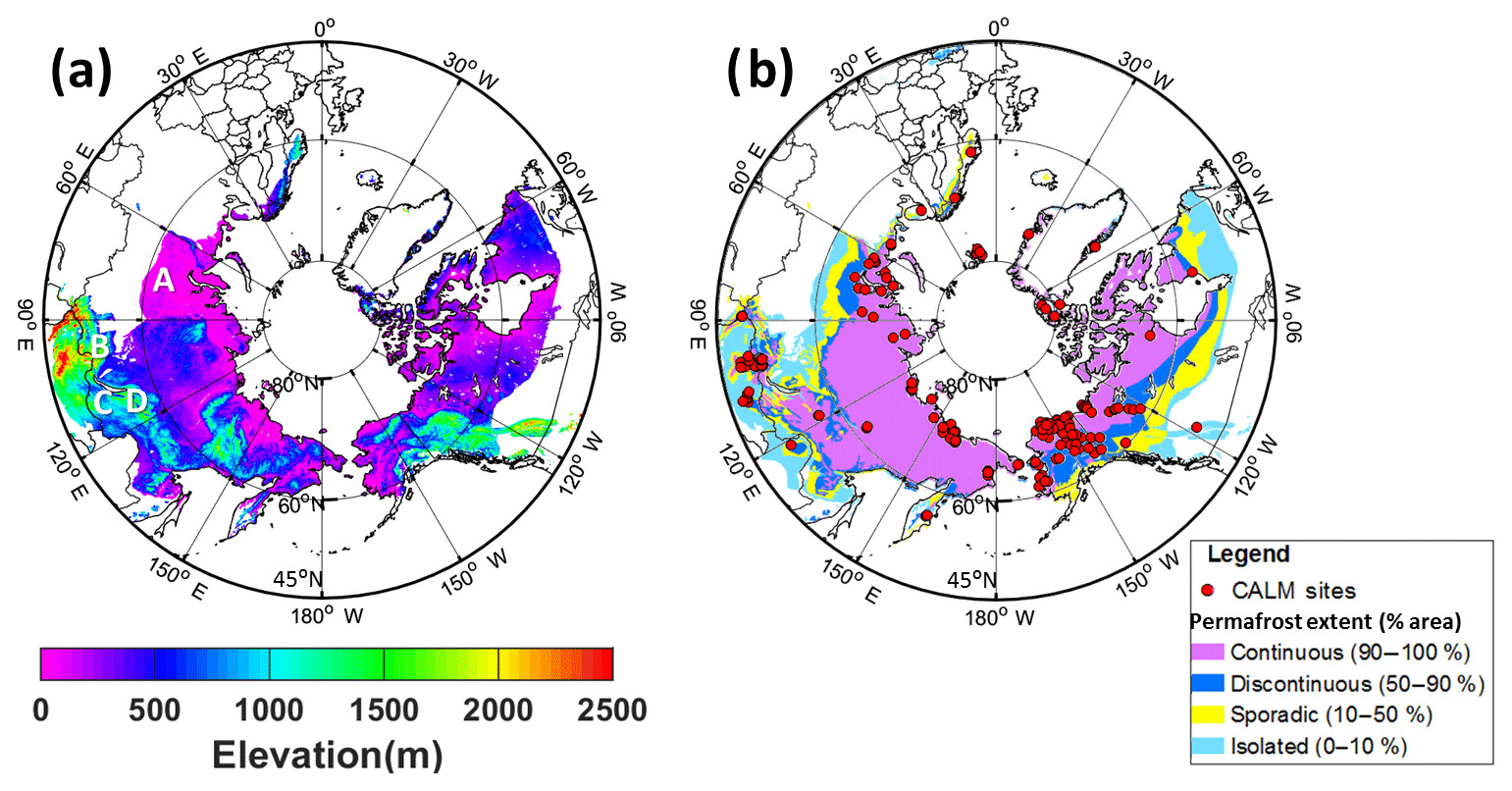
Figure 1 (a) Elevation above mean sea level in the simulation domain, which is defined by the area for which NCSCDv2 data are available. Regions A, B, C, and D are discussed in the text. (b) Permafrost and ground ice conditions adapted from Brown et al. (2002). Red dots represent CALM sites.

We drive the improved CLSM version of Tao et al. (2017) in a land-only (offline) configuration across permafrost areas in the Northern Hemisphere. The simulation domain, shown in Fig. 1a, covers the major permafrost regions of the Northern Hemisphere middle-to-high latitudes for which soil carbon data are available from the Northern Circumpolar Soil Carbon Database version 2 (NCSCDv2, https://bolin.su.se/data/ncscd/, last access: 17 July 2017) (Hugelius et al., 2013a, b). The NCSCDv2 data are used to calculate the CLSM soil thermal properties used in the simulations (Tao et al., 2017). The model simulation covered the period from 1980 to 2017 and was performed at an 81 km² spatial resolution on the 9 km Equal-Area Scalable Earth grid, version 2 (Brodzik et al., 2012).

Surface meteorological forcings were extracted from the MERRA-2 reanalysis data, which are provided at a resolution of 0.5^∘ latitude × 0.625^∘ longitude (Global Modeling and Assimilation Office, GMAO, 2015a, b). At latitudes south of 62.5^∘ N within our simulation domain, the MERRA-2 precipitation forcing used here is informed by gauge measurements from the daily 0.5^∘ global Climate Prediction Center Unified gauge product (Chen et al., 2008) as described in Reichle et al. (2017b). We further rescaled the precipitation to the long-term, seasonally varying climatology of the Global Precipitation Climatology Project version 2.2 product (Huffman et al., 2009). Further details regarding model parameters and forcing inputs are found in Tao et al. (2017).

The model was spun up for 180 years by looping five successive times through the 36-year period of MERRA-2 forcing from 1 January 1980 to 1 January 2016 in order to achieve a quasi-equilibrium state. The spatial terrestrial state variables at the end of the fifth loop were used to initialize the model for the final simulation experiment from 1980 to 2017.

2.2 Remotely sensed ALT from AirMOSS

Radar backscatter measurements are sensitive to changes in the soil dielectric constant (or relative permittivity) which in turn are associated with changes in soil moisture and the soil freeze–thaw state. Based on this relationship, Chen et al. (2019) used the AirMOSS airborne P-band (420–440 MHz) synthetic aperture radar (SAR) observations collected during two campaigns in 2015 to estimate ALT in northern Alaska. As shown in Fig. 2a, the AirMOSS flights originated from Fairbanks International Airport and headed west toward the Seward Peninsula (HUS, KYK, COC), and then they turned back east (KGR) prior to heading north towards the Arctic coast overpassing Ambler (AMB), Ivotuk (IVO), and Atqasuk (ATQ). From there, the flights turned south again, flying over Barrow (BRW, also known as Utqiaġvik), Deadhorse (DHO), and Coldfoot (CFT) en route to Fairbanks. In the present paper, the remotely sensed ALT retrievals are compared with in situ observations and CLSM-simulated ALT.

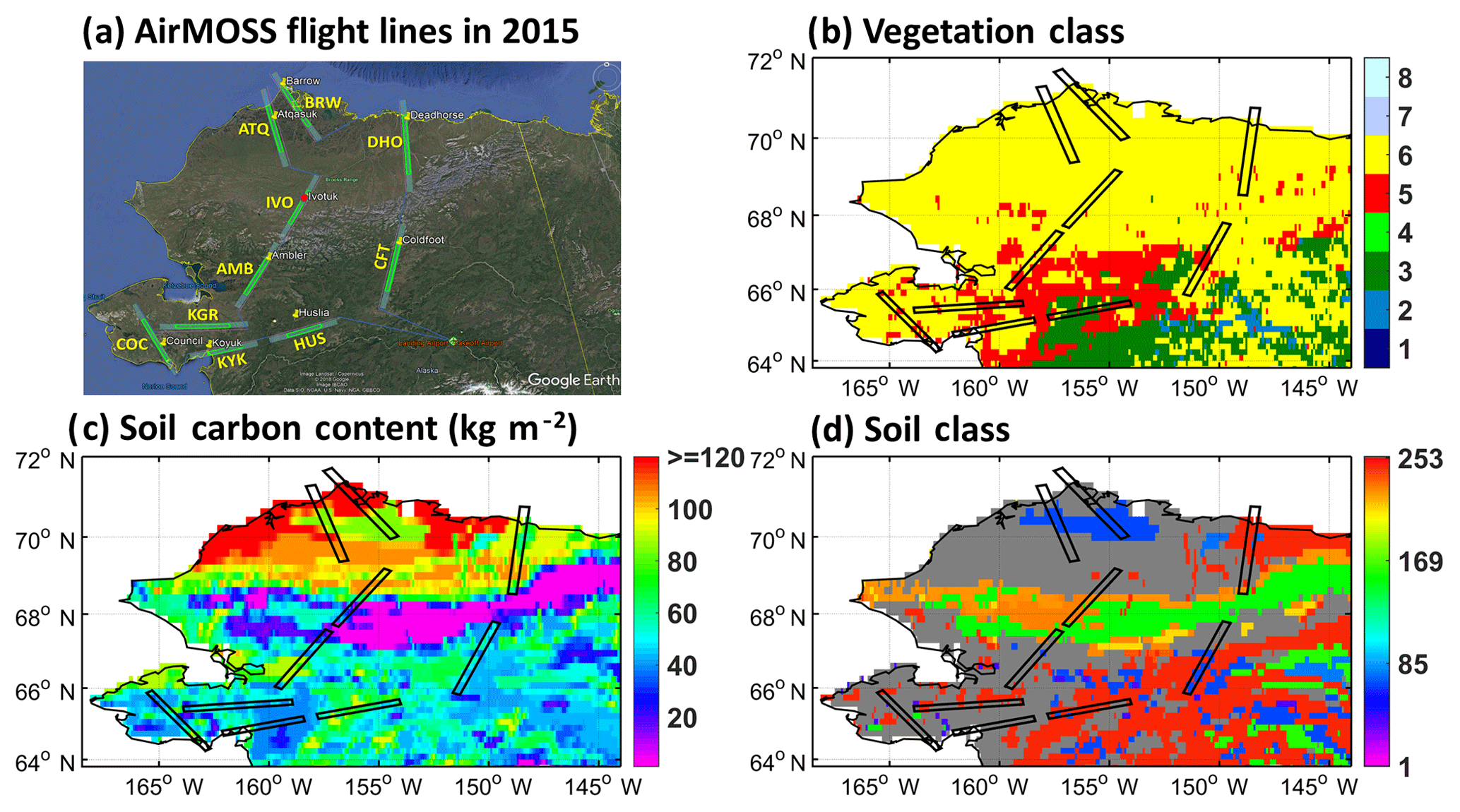
Figure 2 (a) Ten transects of AirMOSS flights conducted in Alaska on 29 August 2015 and 1 October 2015, including HUS (Huslia), KYK (Koyuk), COC (Council), KGR (Kougarok), AMB (Ambler), IVO (Ivotuk), ATQ (Atqasuk), BRW (Barrow), DHO (Deadhorse), and CFT (Coldfoot). Each flight swath width is approximately 15 km. The red dot on IVO illustrates the location of the representative grid cell used and discussed in Sect. 3.2. Background map was adapted from © Google Maps. (b) Vegetation class, (c) soil organic carbon content, and (d) soil class used in CLSM. The eight vegetation classes are (1) broadleaf evergreen trees, (2) broadleaf deciduous trees, (3) needleleaf trees, (4) grassland, (5) broadleaf shrubs, (6) dwarf trees, (7) bare soil, and (8) desert soil. The 253 soil classes include one peat class (no. 253), which is shown in dark grey, and 252 mineral soil classes (De Lannoy et al., 2014).

Chen et al. (2019) used AirMOSS P-band SAR observations at two different times to retrieve active layer properties: (1) acquisitions on 29 August 2015 when the downward thawing process approximately reached its deepest depth (i.e. the bottom of the active layer) and (2) acquisitions on 1 October 2015 when the active layer started to refreeze from the surface while the bottom of the active layer remained thawed. ALT was assumed constant from late August to early October because over this period changes in thawing depth are found typically negligible (Carey and Woo, 2005; R. H. Chen et al., 2016; Zona et al., 2016). Strictly speaking, the radar retrievals represent the approximate thaw depth of the thawed-to-frozen boundary on 29 August 2015 and 1 October 2015. The unknown, true ALT for 2015 might occur later if the thawing continued and the maximum thaw depth occurred after the October flight time. Based on an analysis of in situ observations (not shown), however, it is rare that this occurs, and the subsequent impact on the estimated ALT value would be relatively small in any case. We, therefore, equate the retrieved thaw depth with ALT.

In the retrieval algorithm, Chen et al. (2019) used a three-layer dielectric structure to represent the active layer and underlying permafrost. In their algorithm, the two uppermost layers together constitute the active layer that accounts for a top, unsaturated zone and an underlying, saturated zone. The bottommost (third) layer of the retrieval model structure represents the permafrost. Because the soil moisture at saturation only depends on the porosity of the soil medium, the dielectric constant of the saturated zone in the active layer is assumed constant over the time window. An iterative forward-model inversion scheme was used to simultaneously retrieve the dielectric constants and layer thicknesses of the three-layer dielectric structure from the SAR observations collected on 29 August 2015 and 1 October 2015. Note that the retrieved ALT cannot exceed the radar sensing depth of about 60 cm. This is the depth below which the AirMOSS radar is expected to lose sensitivity to subsurface features, and it is calculated based on the radar system noise floor and calibration accuracy. Therefore, any retrieved ALT larger than 60 cm is expected to have large uncertainties, and the error is further expected to grow linearly as the retrieved values of ALT essentially saturate. This limitation may also lead to underestimates of the actual thaw depth.

In this study, we focus on the retrievals of four flight lines across the Alaska North Slope, including IVO (Ivotuk), ATQ (Atqasuk), BRW (Barrow), and DHO (Deadhorse) as shown in Fig. 2a. These four transects cover areas with light to moderate vegetation. Since the radar scattering model is only applicable to bare surfaces or lightly vegetated tundra areas (Chen et al., 2019), the ALT estimates derived for IVO, ATQ, BRW, and DHO are considered more accurate than ALT retrievals for the remaining transects, which include more vegetated areas. Moreover, some of the southern transects cover discontinuous permafrost where the ALT often exceeds the P-band radar sensing depth of about 60 cm, and thus the retrievals have large uncertainty (Chen et al., 2019).

2.3 Circum-Arctic permafrost conditions and in situ observations of ALT

The permafrost distribution simulated by CLSM is evaluated against the observation-based Circum-Arctic Map of Permafrost and Ground-Ice Conditions (Brown et al., 2002) shown in Fig. 1b. The map is based on the distribution and character of permafrost and ground ice using a physiographic approach. Permafrost conditions are categorized into four classes: continuous (90 %–100 %), discontinuous (50 %–90 %), sporadic (10 %–50 %), and isolated (0 %–10 %), where the numbers in parentheses indicate the area fraction of permafrost extent.

In situ observations of ALT obtained by the CALM network (https://www2.gwu.edu/~calm/, last access: 18 March 2019; Brown et al., 2000) were used to evaluate both the AirMOSS ALT retrievals and CLSM-simulated ALT results. The CALM network provides observations from 1990 to 2017, but few sites have records in the early 1990s. We did not use measurements that were flagged as having been taken too early in the season or under unusual conditions (e.g. after the site was burned or covered with lava, which occurred at sites R30A and R30B in Kamchatka). In total, there are 220 sites located within the CLSM simulation domain (Fig. 1b), and we use 213 sites to evaluate results. Thaw depth measurements are usually made at the end of the thawing season. Most of the CALM sites (129 out of the 213 sites used here) employ a spatially distributed mechanical probing method to measure thaw depths along a transect or across a rectangular grid ranging in size from 10 m × 10 m to 1000 m × 1000 m. At 20 sites, thaw tubes or boreholes are used to measure the thaw depth. At 63 sites, ground temperature measurements from boreholes are used to infer thaw depth. For the remaining site, no information about the measurement method is available. Only point-scale measurements are available from the thaw tube/borehole and ground temperature sites (including the sites in Mongolia).

Table 1 In situ permafrost measurement sites covered by the AirMOSS transects in 2015.

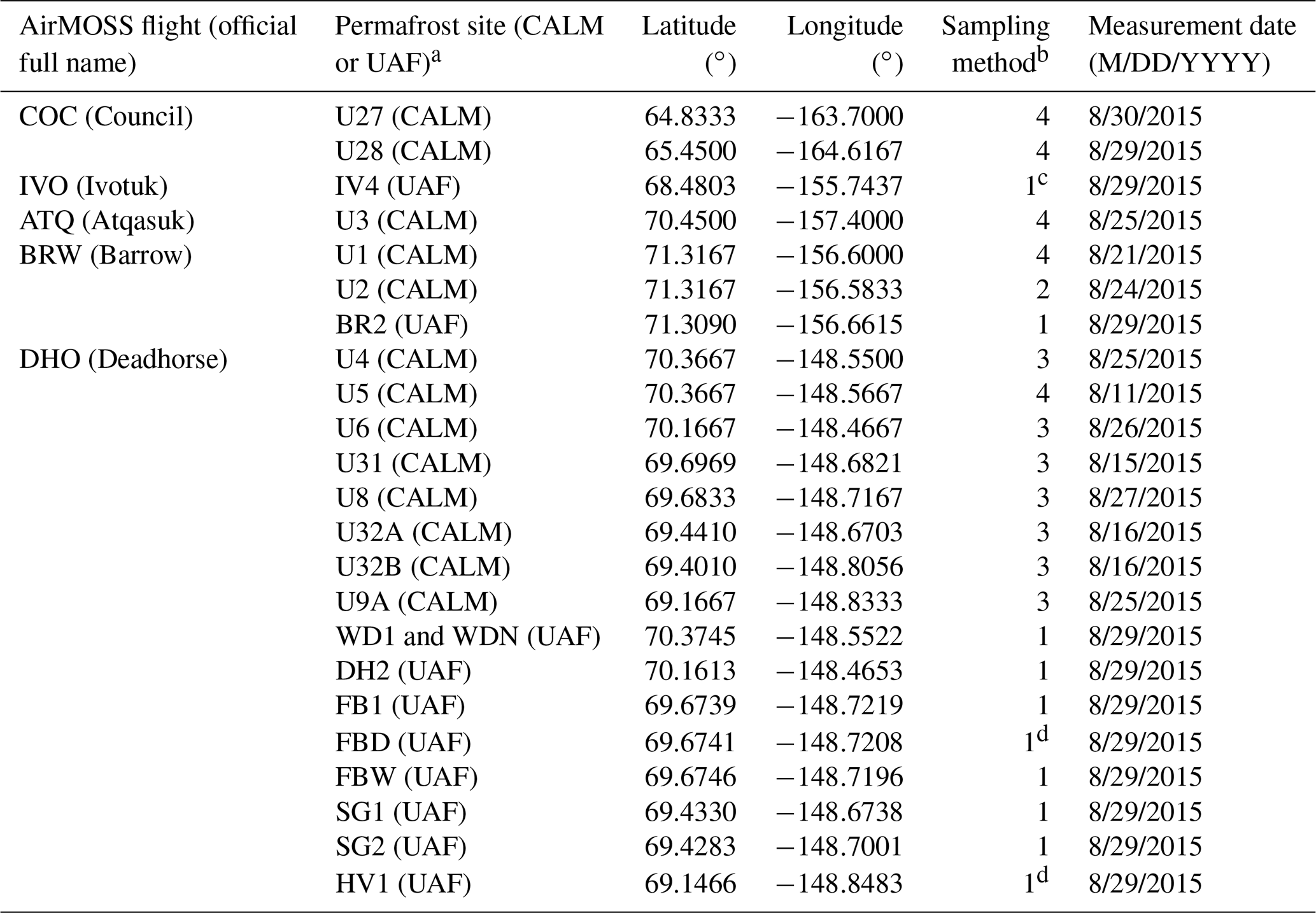
^a CALM: sites from the Circumpolar Active Layer Monitoring (CALM) network; UAF: sites from the Permafrost Laboratory at the University of Alaska Fairbanks. ^b Sampling method: (1) single point; (2) 320 random sampling points within a 10 m × 10m area; (3) 100 m × 100 m grid with a 10 m sampling interval; (4) 1000 m × 1000 m grid with a 100 m sampling interval. ^c Two sensors are installed at IV4. ^d Observations were taken from two conditions, including a frost-boil and an inter-boil area.

In addition, daily in situ observations of soil temperature profiles at 10 Alaskan sites from the Permafrost Laboratory at the University of Alaska Fairbanks (UAF) (http://permafrost.gi.alaska.edu/sites_map, last access: 17 August 2018; Romanovsky et al., 2009) were used to infer thawed-to-frozen depth using the 0 ^∘C degree threshold and to complement the CALM ALT observations in Alaska. Table 1 provides the coordinates and measuring methods of the UAF in situ sites. The UAF measurements were used along with the CALM data to evaluate the ALT estimates derived from the CLSM simulation and the AirMOSS radar observations for the North Slope of Alaska in Sect. 4.1.

3 Methods

3.1 Comparing ALT from in situ observations, AirMOSS retrievals, and CLSM results in Alaska

First, we compare AirMOSS radar retrievals and CLSM simulation results of ALT for 2015 against each other and against in situ observations: (i) we compare the spatial patterns of the AirMOSS retrievals with those of the model-simulated ALT over northern Alaska and (ii) we evaluate the simulated ALT against both the AirMOSS retrievals and in situ observations from the CALM and UAF networks. We rely on several metrics to evaluate the model and radar-retrieval performance, including bias, root mean square error (RMSE), and correlation coefficient (R). The results are discussed in Sect. 4.1.

We conducted the intercomparison at the model scale. The radar retrievals were provided at 2 arcsec × 2 arcsec (roughly 20 m × 60 m in the Arctic) resolution, whereas the CLSM-simulated ALTs are at 81 km². We thus aggregated the AirMOSS retrievals to the CLSM model grid by averaging all the retrieval data points within each 81 km² model grid cell. Only model grid cells that were at least 30 % covered by radar retrievals were used in the comparison. The AirMOSS transects cover several different regions with different climatologic regimes, topography, vegetation, and soil type (Fig. 2). Note that although the vegetation class used in the model (Fig. 2b) suggests the presence of dwarf trees over the Alaska North Slope, the actual satellite-based leaf area index (LAI), vegetation height, greenness fraction, and albedo will still instruct the model that the tree cover there is extremely sparse. The data sources for these vegetation-related boundary conditions can be found in Table 1 of Tao et al. (2017). Overall, the variability of ALT along these transects encompasses the influence of a variety of factors at the regional scale.

The daily UAF in situ soil temperature profile observations on the AirMOSS flight date (29 August 2015) were used to calculate the thawed-to-frozen depth (i.e. approximated ALT). The ALT measurements at all of the 13 CALM sites covered by the AirMOSS transects were obtained in August of 2015 (Table 1). Among them, eight CALM sites obtained ALT measurements slightly earlier than the overflight date (within at most 18 d from 29 August 2015). Nevertheless, we assume that these earlier measurements still represent the thaw depth at the end of August reasonably well. Prior to comparison with the model results and the aggregated radar retrievals, the distributed measurements for a given CALM site (see sampling methods in Table 1) were averaged into a single value. If multiple CALM or UAF sites lay within a single CLSM grid cell, a single spatially averaged observed value was computed for the cell.

We employed the strategy of Schaefer et al. (2015) to handle the uncertainty propagation, i.e. adding in quadrature the uncertainty components from each scale/level involved (see Supplement for a detailed description). For AirMOSS retrievals, the sampling uncertainty of mean ALT at the 81 km² model grid-cell scale is negligible given the large sampling size and the fact that the retrieval uncertainty dominates the overall uncertainty (see Supplement). Here, we use a nominal estimate of 0.15 m to represent the AirMOSS uncertainty (i.e. the average of the lower and upper bound of the actual retrieval uncertainty for individual radar pixels as discussed by Chen et al., 2019).

When comparing in situ measurements with model results at the 81 km² scale (i.e. a point-to-grid comparison), the ultimate measurement uncertainty propagated from the point-scale measurements to the 81 km² scale is, for all intents and purposes, unknown due to a lack of sufficient measurements over the 81 km² scale to compute upscaling errors (see Supplement). We thus show instead the standard deviation of CALM measurements to illustrate, in a highly approximate way, the spatial representativeness error of the in situ measurements – a small (large) standard deviation represents a homogeneous (heterogeneous) area in terms of ALT, meaning that the in situ mean likely can (cannot) represent an average over a larger scale, assuming the site-scale heterogeneity is somewhat transferable to the larger scale. Such transferability might only apply to the largest in situ site scales (e.g. 1000 m × 1000 m) to the model grid scale (81 km²) and is thus, in general, questionable. We thus make no claim here that the standard deviations shown represent true uncertainty levels.

3.2 Idealized experiments

After comparing the spatial patterns of the AirMOSS retrievals with the CLSM-simulated ALT results, we then investigate the factors that affect the spatial variability of ALT through a series of idealized experiments. Specifically, we repeated the simulation along the AirMOSS transects multiple times, each time removing the spatial variation in some aspect of the model forcing or parameters and then quantifying the resulting impact on ALT variability.

For these supplemental simulations, we first identified a grid cell within the IVO transect (shown in Fig. 2a) that represents roughly average (typical) conditions across the 10 different transects. In the first idealized experiment, we then modified the baseline configuration by applying the surface meteorological forcing data from the selected representative grid cell within the IVO transect to all grid cells along all AirMOSS transects. Thus, in this modified simulation (HomF, for homogenized forcing), spatial variability in meteorological forcing is artificially removed. All model parameters related to soil type and vegetation, however, remain spatially variable, matching those in the baseline simulation. In the next idealized experiment (HomF&Veg), we further replaced the vegetation-related parameters (including vegetation class, vegetation height, and time-variable LAI and greenness) along the AirMOSS transects using the corresponding parameters from the representative grid cell, which is characterized by dwarf tree vegetation cover. Thus, in this simulation, spatial variability in both forcing and vegetation is artificially removed.

In a third idealized experiment (HomF&Veg&Soil), spatial variability in soil type and topography-related model parameters is removed along with that of the forcing and vegetation. The homogenized parameters include soil organic carbon content, porosity, saturated hydraulic conductivity, Clapp–Hornberger parameters, wilting point, soil class, sand and clay fraction, vertical decay factor for transmissivity, baseflow parameters, area partitioning parameters, and timescale parameters for moisture transfer (Ducharne et al., 2000; Koster et al., 2000). Here we use an intermediate soil carbon content value (i.e. 40 kg m⁻²) for the homogenization; recall that the carbon content impacts the soil thermal properties (see Sect. 2.1). Our investigation reveals that the model sensitivity to soil carbon content is much larger for lower soil organic carbon content (SOC) than for higher SOC and easily gets saturated for high SOC (i.e. larger than ∼100 kg m⁻²) (not shown). Thus, we trust that 40 kg m⁻² is an appropriate value representing an intermediate SOC condition. All other soil parameters are homogenized to those at the representative grid cell.

Table 2 List of idealized simulation experiments along the AirMOSS transects.

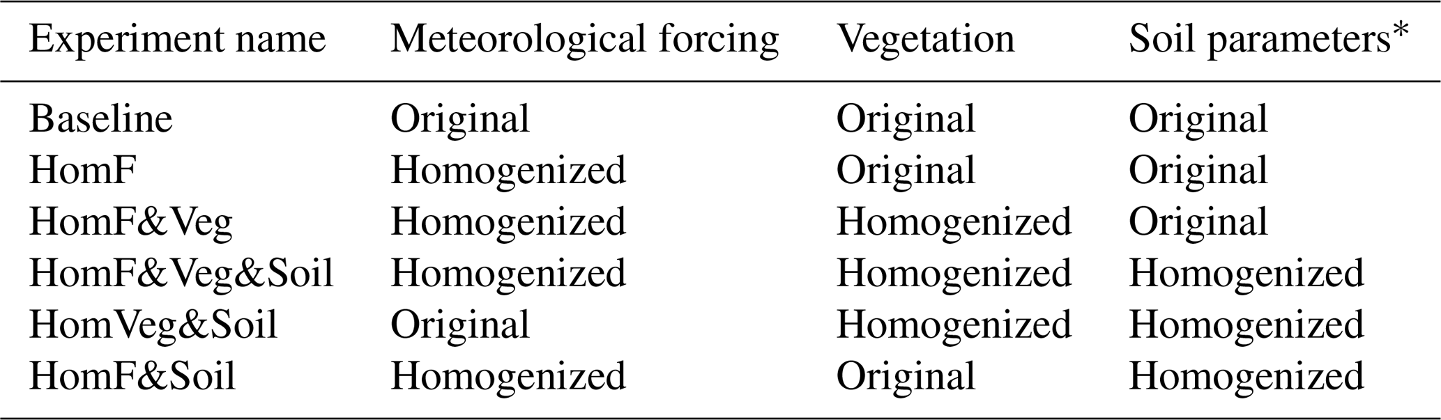
^∗ CLSM soil parameters include soil organic carbon content, porosity, saturated hydraulic conductivity, Clapp–Hornberger parameters, wilting point, soil class, sand and clay fraction, vertical decay factor for transmissivity, baseflow parameters, area partitioning parameters, and timescale parameters for moisture transfer (Koster et al., 2000; Ducharne et al., 2000; Tao et al., 2017).

Finally, we investigate potential nonlinearities by conducting two additional experiments: one in which we homogenized both the vegetation and soil parameters (HomVeg&Soil) and another in which we homogenized both forcing and soil parameters (HomF&Soil). Put differently, in experiment HomVeg&Soil only the forcing varies along the transects, whereas in experiment HomF&Soil, only the vegetation parameters vary along the transects. Combined with the experiment HomF&Veg (in which only soil properties vary along the transects), these three experiments show in a different way how each individual factor (forcing, vegetation, or soil) can contribute to ALT variability. Table 2 provides a summary of these idealized experiments. Taken together, the six experiments (including the baseline) allow us to identify the individual contribution of each factor to the ALT variability along the AirMOSS transects. The results are discussed in Sect. 4.2.

3.3 Quantifying ALT spatio-temporal characteristics

In Sect. 4.3 we quantify the large-scale characteristics of ALT over the Northern Hemisphere for the current climate (1980–2017) as determined by the response of the land model to 38 years of MERRA-2 forcing (Sect. 2.1). The output from this multi-decadal, offline simulation allows the characterization of permafrost dynamics at each grid cell. In particular, we can compute a number of relevant ALT statistics, including mean, standard deviation, and skewness, from the diagnosed yearly values at each cell, and we can examine how these statistics relate to those of MERRA-2 forcing data (particularly the mean annual air temperature, MAAT) over the last 38 years.

Besides MAAT statistics, we also consider the evolution of the air temperature during the warm season in terms of the energy it could provide to the land surface and thus to the determination of ALT. A simple surrogate for the total warm-season energy in year N can be computed from daily-averaged air temperature, T_air(t), and the freezing temperature, T_f (0 ^∘C degree), as follows:

$$\begin{array}{}\text{(2)}& T_{\mathrm{cum}}\left(N\right)=\sum _{t=\mathrm{1}}^{t=M}{T}_{\mathrm{pos}}\left(t\right),\end{array}$$

where

$$\begin{array}{}\text{(3)}& T_{\mathrm{pos}}\left(t\right)=\left\{\begin{array}{ll}{T}_{\mathrm{air}}\left(t\right)-T_f& \text{if }{T}_{air}\left(t\right)>T_f\\ \mathrm{0}& \text{if }{T}_{\mathrm{air}}\left(t\right)\le T_f\end{array}\right..\end{array}$$

The index t in Eq. (2) for year N starts with a value of 1 on 1 September of the year (N−1) and ends with a value of M on 31 August of year N. The number of days M is 365 or 366 depending on the presence of a leap year. Note the air temperature throughout this study means the near-surface air temperature (i.e. 2 m above the displacement height) derived from MERRA-2.

We first computed the correlation coefficient (R) between the annual time series of ALT and $\sqrt{T_{\mathrm{cum}}}$ and between the annual time series of ALT and maximum SWE (SWE_max) to quantify the degree to which variations of ALT can be explained solely by air temperature or by snow mass. Then, to quantify the joint contributions of $\sqrt{T_{\mathrm{cum}}}$ and SWE_max, we performed a multiple linear regression analysis by fitting the equation

$$\begin{array}{}\text{(4)}& \mathrm{ALT}=a_{\mathrm{0}}+a_{\mathrm{1}}\sqrt{T_{\mathrm{cum}}}+a_{\mathrm{2}}{\mathrm{SWE}}_{\max }\end{array}$$

to the available data. The correlation coefficient relating ALT to $\sqrt{T_{\mathrm{cum}}}$ and SWE_max is the square root of the coefficient of multiple determination (R²) obtained through fitting Eq. (4). This equation is similar in form to the common degree-day model for predicting ALT from accumulated degree days of thaw based on the Stefan solution (e.g. Shiklomanov and Nelson, 2002; Zhang et al., 2005; Riseborough et al., 2008; Shiklomanov et al., 2010). Here, however, we constructed Eq. (4) for a different purpose: to explore how much of the temporal variability of ALT can be jointly explained by snow mass and above-freezing air temperature. Before calculating these correlation coefficients, we removed the linear trend within ALT, T_cum, and SWE_max to avoid potentially exaggerating the correlation due to an underlying trend. The results are discussed in Sect. 4.3.

3.4 Evaluating simulated Northern Hemisphere permafrost extent and ALT

We first evaluated the simulated permafrost extent against the observation-based permafrost map (Brown et al., 2002, as shown in Fig. 1b). Note the model's description of permafrost is binary – either permafrost exists across a grid cell or it is completely absent. We cannot then expect an exact comparison to a specification of isolated permafrost (0 %–10 % of area by definition) or even, to a lesser extent, sporadic permafrost (10 %–50 % of area by definition). Therefore, we compared our simulated permafrost area with that of the total area of continuous, discontinuous, and sporadic permafrost area together from Brown et al. (2002) and computed the percentage error relative to the observation-based area (i.e. the total area of continuous, discontinuous, and sporadic permafrost regions). We also compared our simulated permafrost area against the total area of only continuous and discontinuous permafrost regions.

Further, the CALM network of in situ ALT measurements (Sect. 2.3) allows a quantitative evaluation of the simulated ALTs for the grid cells containing measurement sites. Our comparisons here focus on both multi-year annual ALTs and the average (climatological) ALT at the 81 km² scale of CLSM data. To ensure a consistent comparison, we average the simulated ALTs only over the years for which observations are available. As noted in Sect. 3.1 and the Supplement, the uncertainty of the CALM ALT measurements in the context of evaluating grid-cell-scale model results theoretically involves uncertainty derived from probing point measurement uncertainty, site-scale mean uncertainty, and upscaling errors in going from the site scale to the model scale. This latter uncertainty, in particular, is unknown. In our figures (in Sect. 4.4) we show the standard deviation of the observed ALT as a very crude surrogate for the spatial representativeness error associated with the point-to-grid comparison. As before, we make no claim here that the standard deviations shown represent the relevant statistical uncertainty. The results are discussed in Sect. 4.4.

4 Results

4.1 Simulated ALT versus in situ measurements and AirMOSS retrievals in Alaska

In this section, we compare the simulated ALT and the AirMOSS ALT retrievals at the 81 km² model resolution. Note that Chen et al. (2019) provide maps of the AirMOSS retrievals and an evaluation versus in situ measurements at the native (20 by 60 m) scale of the retrievals.

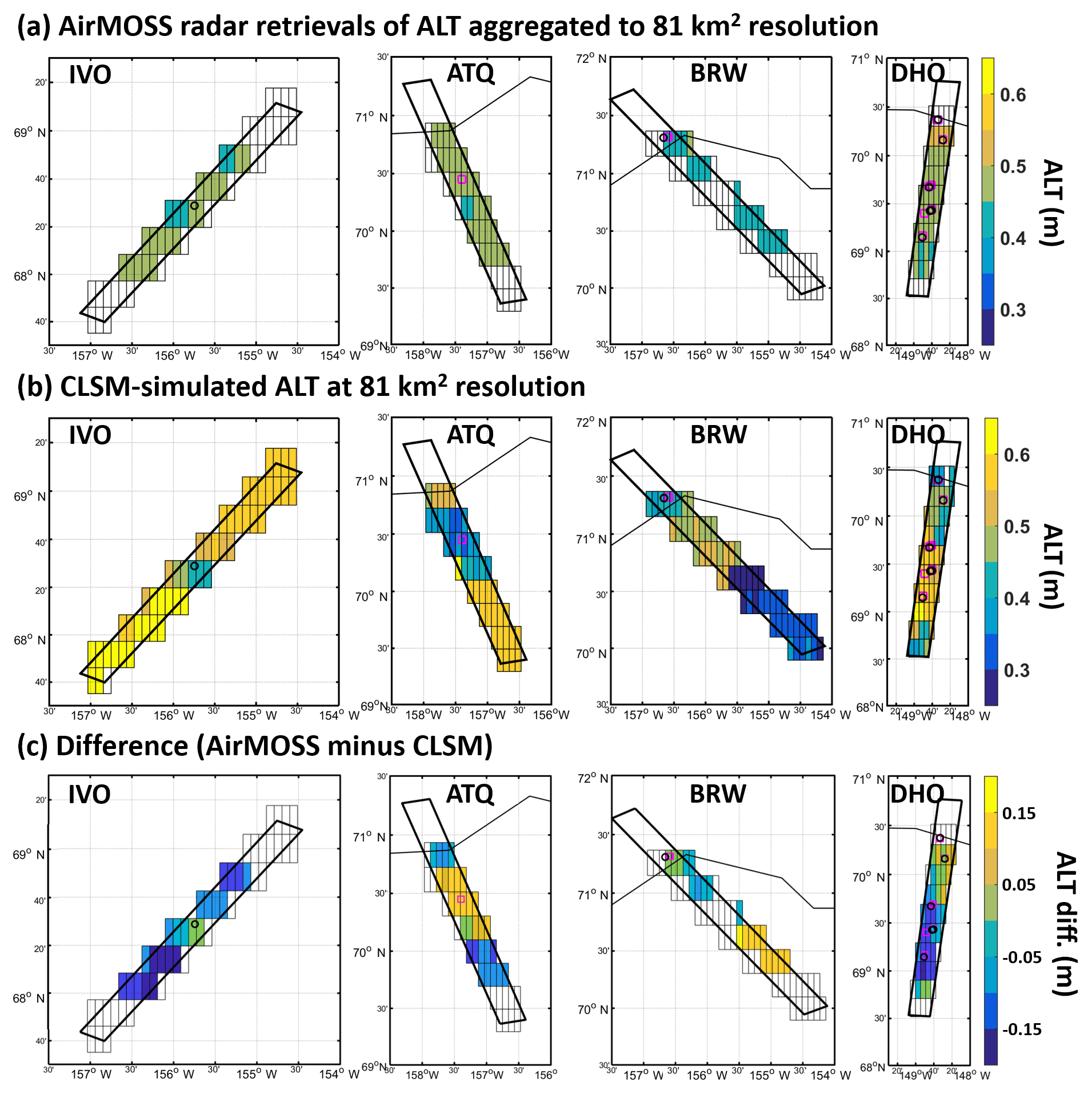
Figure 3 (a) Radar retrievals of ALT derived from P-band radar observations on 29 August 2015 and 1 October 2015 for IVO, ATQ, BRW, and DHO, aggregated to 81 km² model grid cells. (b) CLSM-simulated ALT. (c) Difference between the aggregated ALT retrievals and the CLSM-simulated results. Magenta squares represent CALM sites covered by the flight swath, whereas black circles represent UAF sites.

Figure 3 compares the spatial pattern of AirMOSS ALT retrievals and CLSM-simulated results. Generally, the patterns of the AirMOSS retrievals and CLSM results are quite different. For example, the AirMOSS-retrieved ALT is greater in the northern portion of the DHO transect than in the southern portion (Fig. 3a), whereas this pattern is largely reversed in the simulated ALT for DHO (Fig. 3b). Across all transects, there are portions where the AirMOSS ALT is less than the CLSM-simulated ALT and portions where the AirMOSS ALT is greater (Fig. 3c), though it should be noted that the differences in Fig. 3c are generally less than the assumed uncertainty of 0.l5 m (see Sect. 3.1). Generally, the CLSM-simulated ALT shows relatively larger spatial variability (0.35–0.85 m) than the AirMOSS retrievals (0.4–0.6 m). The AirMOSS ALT exhibits some spatial variability at the native resolution (see Chen et al., 2019), but much of this variability averages out during the aggregation to the coarse model grid (Fig. 3a). Variations of the simulated ALT within a single transect (Fig. 3a) are predominantly induced by changes in soil type (indicated in Fig. 2c and d). In essence, the higher the organic carbon content within the soil, the smaller the simulated ALT due to slower heat transfer associated with lower thermal conductivity, higher porosity, heat capacity, etc. (Tao et al., 2017). See also Sect. 4.2 for a discussion of the influence of soil texture on the spatial pattern of ALT.

Figure 4 (a) ALT observations (red) for 2015 from CALM and UAF sites covered by AirMOSS swaths and from radar retrievals aggregated to 81 km² grid cells (green), and CLSM-simulated ALT at 81 km² (blue). The short name of the corresponding covering swath is shown on the top (see also Fig. 2a). Error bars represent the standard deviation for multiple observations at in situ sites. No standard deviations are provided for UAF sites since single-point measurements were deployed. Averaged values were provided if multiple sites appear within a same model grid cell (e.g. U1&U2, U4&U5, WD1&WD2, FB1&FBD&FBW, and SG1&SG2). The sites are arranged aligning with the flight direction. (b) CLSM estimates of ALT for 2015 versus in situ measurements with error bars indicating the standard deviation as in panel (a). (c) Same as panel (b) but versus aggregated AirMOSS ALT at the model scale. The error bars here represent the uncertainty for radar retrieval means within each 81 km² grid cell as explained in Sect. 3.1. Corresponding estimates of CLSM uncertainty, which are presumably large, are not shown in the figure.

Next, we compare the simulated ALT in 2015 with in situ observations from the CALM and UAF sites that are collocated with the AirMOSS transects (Sect. 3.1). Figure 4a and b show that the CLSM-simulated ALTs agree with the in situ observations with an overall mean bias of −0.05 m and an RMSE of 0.17 m. The most significant discrepancies between the CLSM-simulated ALT and in situ measurements are at U6, U31, FB1&FBD&FBW (Fig. 4a), where the simulated ALT underestimates the in situ measurements by 0.25–0.28 m; and at U28, where the simulated ALT overestimates the in situ ALT by 0.27 m. Nevertheless, the scatter in Fig. 4b is large, and the corresponding correlation coefficient is quite weak (0.27).

Table 3 Evaluation metrics for model-simulated ALT and AirMOSS retrievals for 2015.

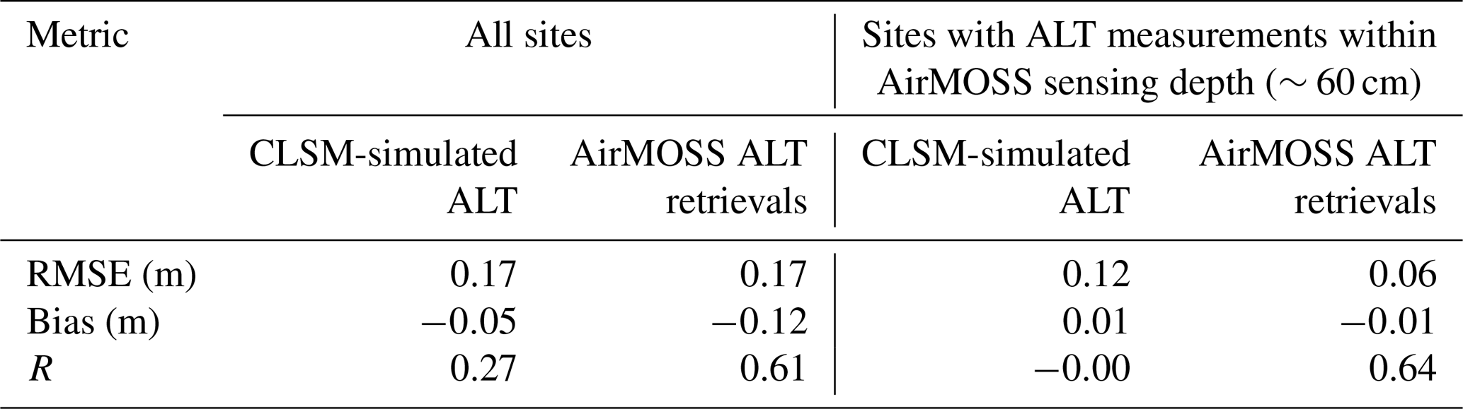
The AirMOSS ALT radar retrievals, for their part, again averaged to the 81 km² model resolution (Sect. 2.2), show less spatial variability than the observations (Fig. 4a). The largest error for the AirMOSS retrievals at the model scale is also at FB1&FBD&FBW, where the retrievals significantly underestimate the observed in situ ALT by 0.38 m. Note that radar retrievals at the 81 km² scale are not available at some sites because of our imposed 30 % filling restriction. Although the AirMOSS ALT retrievals generally underestimate the in situ ALT measurements (as shown in Fig. 4a), the retrievals tend to be more consistent with the observations when the in situ measurements are within the ∼60 cm sensing depth of the P-band radar data, as indicated in Table 3. Specifically, excluding the sites with in situ ALT measurements that exceed the AirMOSS sensing depth of ∼60 cm, the overall mean bias for the AirMOSS retrievals at the 81 km² scale drops to −0.01 m, and the correlation coefficient increases to 0.64. In contrast, the CLSM simulation results show a bias of 0.01 m and a zero correlation coefficient at these sites.

Nevertheless, as noted in Sect. 3.1, given that the upscaling errors in going from the CALM site scale to the model scale are unknown and the fact that the standard deviation of these measurements (as shown by error bars in Fig. 4a and b) indicates large representativeness errors of the in situ measurements, the point-to-grid comparison result is hard to quantify. In this regard, the AirMOSS retrievals aggregated to the same scale as model results provide a comparable counterpart for evaluation. Figure 4c further shows that the CLSM-simulated ALT agrees well with the AirMOSS ALT retrievals to within the measurement uncertainty of 0.15 m at all the site-located model grid cells. Indeed as Fig. 3c illustrated, the differences between simulated ALT and the AirMOSS retrievals over all the transects examined here are generally below the measurement uncertainty of 0.15 m.

4.2 Sources of ALT spatial variability: results from idealized experiments

Here we investigate the specific factors that drive ALT spatial variability along all 10 of the AirMOSS transects (Fig. 2a). For this analysis, the simulated ALT estimates were aggregated across the width of the radar swath (compare Fig. 3). Figure 5a illustrates that the simulated ALT captures the spatial variability exhibited by the in situ measurements. This conclusion is, however, very tentative given the limited number of in situ ALT observations.

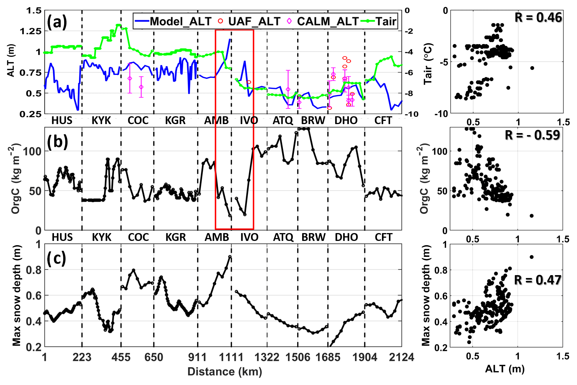
Figure 5 (a) CLSM-simulated ALT (thawed-to-frozen depth) on 29 August 2015 along the AirMOSS flight transects. In situ ALT observations from UAF and CALM are shown as red circles and magenta diamonds, respectively. Averaged air temperature at 2 m (Tair) from the preceding annual period (i.e. 1 September 2014 to 31 August 2015) is shown in green with the scale on the right ordinate. (b) Organic carbon content and (c) maximum snow depth during the preceding annual period (again from 1 September 2014 to 31 August 2015). The red rectangle across panels (a) and (b) highlights a portion of the domain that shows anti-correlation between organic carbon content and modelled ALT (see Sect. 4.2). The abscissa in panel (c) provides cumulative distances in units of kilometres along the transects.

The simulated ALT is shallowest in the northern transects (ATQ, BRW, and DHO) and deepest in the southeastern transects (KYK, COC, KGR, and AMB). This pattern correlates somewhat (R=0.46) with that of the mean screen-level (2 m) air temperature (Tair) for the preceding 12-month period (i.e. from 1 September 2014 to 31 August 2015) from MERRA-2 (green line in Fig. 5a). The soil carbon content, by contrast, appears anti-correlated ($R=-\mathrm{0.59}$) with the simulated ALT, as exemplified by the transect portions within the red box (Fig. 5a and b). Such a correlation presumably reflects the fact that soil with high organic carbon content has low thermal conductivity, which hinders heat transfer from the surface to the deeper soil in the summertime, thus resulting in a relatively smaller ALT. In addition, heat transfer is slowed by a higher effective heat capacity associated with higher organic carbon content – not from the carbon itself but from the extra water that can be held in the soil due to the increased porosity. The maximum snow depth (Fig. 5c) displays a positive correlation with ALT (R=0.47), reflecting, at least in part, the fact that subsurface soil temperatures remain relatively insulated under thick and persistent snow cover, which reduces heat transfer out of the soil column during the wintertime and hence facilitates a deeper thawing during the summer and thus a deeper ALT.

The correlations in Fig. 5 suggest (without proving causality) that for the model, surface meteorological forcing (including air temperature and precipitation) and soil type are important drivers of ALT variability along the AirMOSS transects. However, the relatively low values of the correlations indicate that a simple linear relationship cannot explain the mutual control that these variables exert on ALT spatial variability. In the remainder of this section, we use a series of idealized model simulations (as described in Sect. 3.2) to better quantify the relative impacts of these driving factors along the AirMOSS transects.

The results of the idealized experiments are shown in Fig. 6. The above-mentioned, large-scale spatial variation of ALT in the baseline simulation, with larger values in the southeastern transects (KYK, COC, and KGR) and lower values in the northern transects (ATQ, BRW, and DHO), is absent after homogenizing the meteorological forcing (HomF; Fig. 6a). Experiment HomF correspondingly has much less spatial variation in the temperature of the top soil layer than does the baseline simulation (Fig. 6b). In addition, homogenizing the forcing (which includes snowfall) significantly reduces the variability in maximum snow depth along the AirMOSS transects (Fig. 6c). These results indicate that, in the model, meteorological forcing exerts the dominant control over the spatial patterns of ALT, the temperature in the top soil layer, and snow depth at the regional scale, as expected.

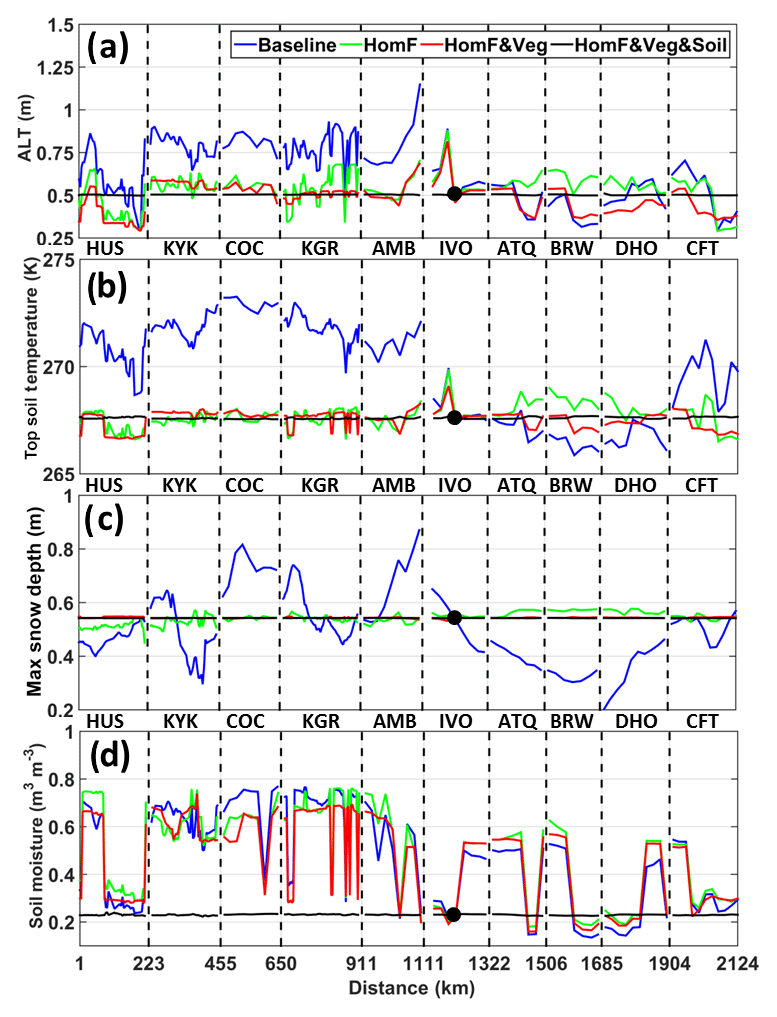
Figure 6 (a) CLSM-simulated ALT (thawed-to-frozen depth) on the flight date (i.e. 29 August 2015) from the top four experiments listed in Table 2, (b) simulated top layer soil temperature on the flight date, (c) maximum snow depth the during the preceding annual period (i.e. from 1 September 2014 to 31 August 2015), and (d) soil moisture within the soil profile on the flight date along the connected transects for the four experiments. The black dot indicates the representative location within the IVO transect from which the forcing, vegetation, and/or soil data are used to homogenize the inputs in the idealized experiments. By construction, all simulations provide identical results at this representative location.

Homogenizing the vegetation attributes in addition to the forcing (HomF&Veg) results in ALT differences (relative to HomF) primarily along the northern transects (ATQ, BRW, and DHO). Along these transects, homogenizing the vegetation parameters (including LAI and tree height) to those of the representative grid cell within the IVO transect results in generally shallower ALT. This is because the generally lower albedo of the taller and leafier trees (representative of the IVO transect) during the snow season resulted in increased snowmelt and thus reduced snowpack during the snow season (compare the green and red curves in Fig. 6c), thereby reducing the thermal insulation of the wintertime ground. With reduced insulation, cold season ground temperatures dropped, making it more difficult for temperatures to recover during summer (Tao et al., 2017).

As might be expected, the simulation in which soil properties are homogenized in conjunction with forcing and vegetation (i.e. HomF&Veg&Soil) essentially eliminates all remaining spatial variability in ALT, snow depth, and soil temperature. Owing to the strong control of soil-type-related parameters (see Sect. 3.2 and Table 2) on soil moisture, spatial variability in soil moisture remains high in HomF and HomF&Veg and is only eliminated once these soil-type-related parameters are homogenized (Fig. 6d), which explains the abrupt changes shown in Fig. 3c as mentioned in Sect. 3.1. (Note that to maintain consistency with the hardwired scaling factors for snow-free albedo within the model (Mahanama et al., 2015) we still used the original, vegetation-related parameters to calculate surface albedo during snow-free conditions along the transects. This is likely the cause of the few tiny bumps seen in Fig. 6a for HomF&Veg&Soil.)

An alternative view of these results is provided in Fig. 7a, which shows the (spatial) standard deviation of ALT along the AirMOSS transects for each of the above experiments. Homogenizing the meteorological forcing data results in a significant reduction of the ALT standard deviation (from 0.16 to 0.10). Additionally homogenizing the vegetation only reduces the ALT standard deviation slightly (from 0.10 to 0.09). The remaining ALT variability is eliminated through the additional homogenization of the soil-type-related parameters (HomF&Veg&Soil), which emerge as another important driver of ALT variability along the AirMOSS transects. Note that the ALT variability associated with soil type is generally realized at smaller spatial scales than that associated with the meteorological forcing discussed earlier regarding Fig. 6a. The impact of potential nonlinearities is examined in Fig. 7b, which shows the individual impact of vegetation, soil, and forcing heterogeneity on the ALT standard deviation along the transects, with the other inputs having been homogenized. The graphic confirms that the meteorological forcing is the dominant driver of ALT spatial variability in our modelling system, followed by the soil-type-related parameters and the vegetation parameters.

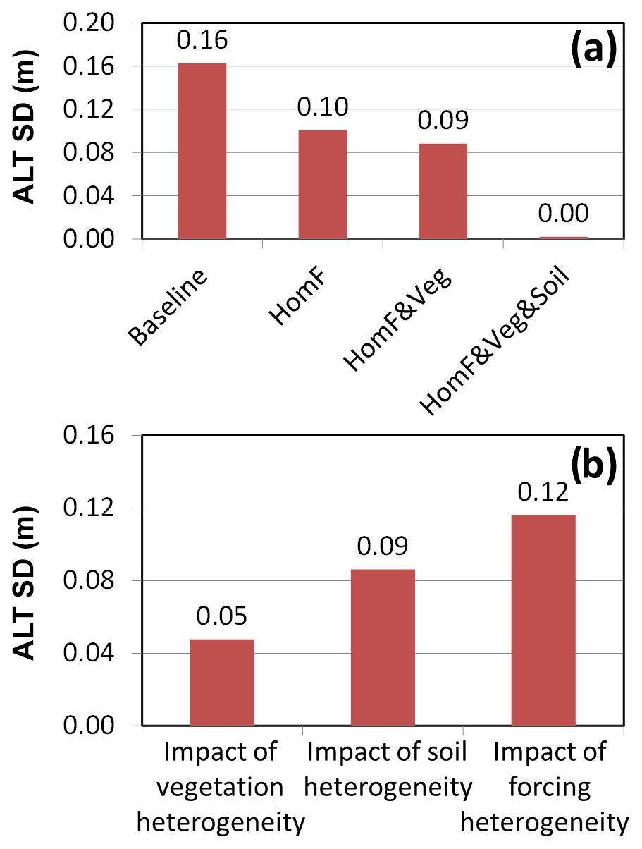
Figure 7 (a) Standard deviation of ALT along the AirMOSS transects from the top four experiments listed in Table 2. (b) The individual impact (or contribution) from heterogeneous vegetation, soil type, and meteorological forcing, respectively. For instance, the impact of vegetation (or soil, or forcing) heterogeneity is the ALT standard deviation along the transects from HomF&Soil (or HomF&Veg, or HomVeg&Soil).

Note that in Fig. 6a the soil impact on ALT (the difference between HomF&Veg&Soil in black and HomF&Veg in red) appears smaller than that of the vegetation (the difference between HomF in green and HomF&Veg in red) over the northern transects (ATQ, BRW, and DHO). Even so, Fig. 7b shows that, in terms of the integrated impact along all the transects, the soil influence clearly outweighs the influence of vegetation – at several other transects, including HUS, KYK, COC, AMB, IVO and the first half of ATQ (where vegetation conditions might be similar to those used for homogenizing), the changes in vegetation parameters do not have much impact.

4.3 Spatio-temporal characteristics of ALT across the Northern Hemisphere

Figure 8a shows the distribution of mean ALT over the modelling domain, and Fig. 8b shows the ALT standard deviation in time over the 38-year period. As might be expected, ALT tends to increase with distance from the pole, with the largest values found in Mongolia and near the southern portion of the Hudson Bay, though there are areas (e.g. just north of 60^∘ N at ∼120^∘ E) with local minima that break this pattern. The largest ALT standard deviations (red colour in Fig. 8b) are found mainly in discontinuous and sporadic permafrost regions (see Fig. 1b) where ALTs are deeper on average than that in the continuous permafrost region. Figure 8c provides the skewness of the temporal distribution. Though there are some exceptions, by and large, the skewness is positive in most permafrost regions, suggesting that the largest positive ALT anomalies tend to be of greater magnitude than the largest negative anomalies.

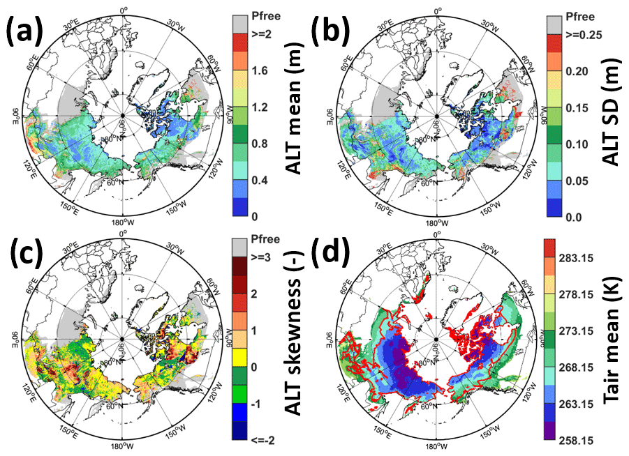
Figure 8 (a) Mean, (b) standard deviation, and (c) skewness of CLSM-simulated ALT over the 38 years (1980–2017). Grey indicates permafrost-free (Pfree) areas in the simulation. (d) The 38-year averaged MERRA-2 annual atmospheric temperature at 2 m above displacement height (Tair). The red boundary outlines the continuous and discontinuous permafrost regions according to Brown et al. (2002).

Figure 8d displays the average of annual mean 2 m air temperature as derived from MERRA-2. The observed continuous and discontinuous permafrost areas shown in Fig. 1b are well confined within the cold side of the 0 ^∘C (273.15 K) isotherm in the mean air temperature map (Fig. 8d). For the most part, the observed sporadic and isolated permafrost regions of Fig. 1b also lie on the cold side of the 0 ^∘C isotherm. The consistency with this isotherm, however, is not as clearly present in the simulated permafrost extent (i.e. the extent of the non-grey and non-white areas in Fig. 8a).

The relationship between the spatio-temporal characteristics of simulated ALT and air temperature forcing has been investigated before in many studies at the site to the landscape scale (e.g. Klene et al., 2001; Shiklomanov and Nelson, 2002; Zhang et al., 2005; Juliussen and Humlum, 2007) and at the regional scale (e.g. Anisimov et al., 2007). Here we simply analyse the correlation coefficient between ALT and two variables: the proxy of total energy input into the ground (i.e. $\sqrt{T_{\mathrm{cum}}}$; see Sect. 3.3) and the maximum SWE. Our goal is to explore how much of the spatio-temporal variability of ALT across the globe can be jointly explained by these two variables.

Figure 9a shows a map of the correlation coefficient between the 37-year time series (i.e. from September 1980 through August 2017) of $\sqrt{T_{\mathrm{cum}}}$ and the corresponding time series of simulated ALT. The areas with p values larger than 0.05, which indicate correlations that are not statistically different from zero at the 95 % confidence level, are shown as green. Figure 9a demonstrates that most permafrost regions indeed have significant positive correlations (red colours) between ALT and $\sqrt{T_{\mathrm{cum}}}$. Clearly, in these regions, air temperature exerts a dominant control on year-to-year ALT variability.

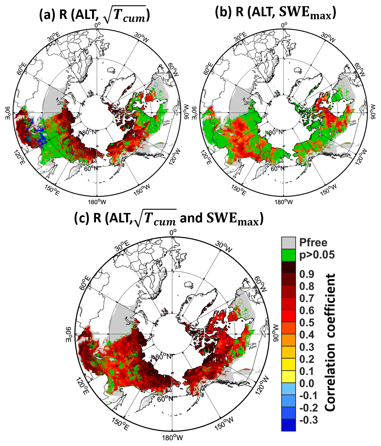
Figure 9 Correlation coefficient between (a) ALT and square root of the effective accumulated air temperature ($\sqrt{T_{\mathrm{cum}}}$) and (b) ALT and maximum SWE (SWE_max) from the preceding September to the present August over the period 1980–2017. (c) Multi-variable coefficient of correlation for a fitted multiple linear regression model between ALT and $\sqrt{T_{\mathrm{cum}}}$ and SWE_max. Areas that have a p value larger than 0.05 (i.e. statistically insignificant correlation) are masked in green. Grey indicates permafrost-free (Pfree) areas in the simulation.

However, not all regions exhibit a significant correlation; other variable(s) must also be exerting control on interannual ALT variability. One reasonable candidate variable is snowpack. As noted above, snow acts as a thermal insulator – regions with thicker snowpack are better able to insulate the ground from becoming too cold during winter, thereby supporting higher subsurface temperatures during non-winter months. Variable, but often thick, snowpack is in fact common in the areas of Fig. 9a that show a low (green) or negative (blue) correlation between ALT and $\sqrt{T_{\mathrm{cum}}}$ – areas such as central Siberia, the southern part of eastern Siberia, and a vast region in Canada surrounding the Hudson Bay, as well as other small areas that appear in high mountains or on the windward side of the mountains (e.g. locations B, C and D in Fig. 1a).

In Fig. 9b we show the correlation coefficient between the time series of ALT and the maximum SWE (SWE_max) during the preceding winter. A positive correlation is seen in many areas, most notably in areas with a poor or negative correlation between ALT and $\sqrt{T_{\mathrm{cum}}}$ (Fig. 9a) – for example, just west of the Hudson Bay and along a zonal band at 60^∘ N in Russia. Apparently, in these areas, the impacts of snow physics on ALT outweigh the impacts of lumped energy input ($\sqrt{T_{\mathrm{cum}}}$). In some other areas ALT correlates positively with both $\sqrt{T_{\mathrm{cum}}}$ and SWE_max. Figure 9c shows how the resulting coefficient of multiple correlation varies in space. High correlations largely blanket the modelled area. That is, over most of the area examined, a substantial portion of the year-to-year variability of ALT can be explained by joint variations in $\sqrt{T_{\mathrm{cum}}}$ and SWE_max. Even so, a few limited areas still exhibit low correlations (p>0.05, green colour in Fig. 9c). Some of these areas are in mountainous regions, for instance the Eastern Siberian (Ostsibirisches) Bergland, where more complex environmental controls might be playing a dominant role. In addition, MERRA-2 snow forcing might be severely erroneous in these regions.

4.4 Evaluation of simulated permafrost extent and ALT across the Northern Hemisphere

Qualitatively, the simulated permafrost extent (Fig. 8a) generally shows reasonable agreement with the observation-based permafrost map in Fig. 1b, especially for the continuous permafrost regions. This is shown explicitly in Fig. 10a. The main deficiency in the simulation results is the failure to capture a large area of permafrost in western Siberia (labelled as A in Fig. 1a). The reasons for this particular deficiency are unclear. One possible reason is that the permafrost in western Siberia is characterized as an ecosystem-protected permafrost zone (Shur and Jorgenson, 2007) where a thick moss-organic layer (i.e. moss-dominated mires; Anisimov and Reneva, 2006; Anisimov, 2007; Peregon et al., 2009) protects the permafrost below from thawing under a warm air temperature. This is mainly attributed to the low thermal conductivity of the organic layer in summer, which strongly insulates the permafrost from the warm atmosphere, and the high thermal conductivity of the frozen organic layer in winter, which allows cold temperature penetration from above, provided the snowpack is not too thick (Nicolsky et al., 2007; Jafarov and Schaefer, 2016). This mechanism is lacking in the current version of CLSM (Tao et al., 2017). Thus, improving the model through a better representation of thermal processes in an organic layer above the soil column in combination with initializing the simulation with a sufficiently cold soil temperature should improve the simulation results. This work is reserved for a future study.

Figure 10 (a) Four comparison categories include (1) blue – CLSM collocates permafrost with the observation-based permafrost map of Brown et al. (2002) as either continuous, discontinuous, or sporadic permafrost; (2) green – CLSM has no permafrost, but the observation-based permafrost map does as either continuous, discontinuous, or sporadic types; (3) red – CLSM does have permafrost, but the observation-based permafrost map does not or contains isolated permafrost; and (4) grey – CLSM has no permafrost and neither does the observation-based permafrost map (except for isolated permafrost). (b) Area-weighted average of ALT as simulated by CLSM for the four different permafrost types.

Another possible reason for the poor skill in western Siberia is that the model initial conditions there were too warm, although MERRA-2 appears to underestimate summer air temperatures in this region (Draper et al., 2018; their Fig. 7e). Note that some other global models, such as CLM3 and the Community Climate System Model version 3 (CCSM3) as reported in Lawrence et al. (2012), also missed this area of permafrost and that updated versions of these models (i.e. CLM4 and CCSM4) showed improved performance in this regard (Lawrence et al., 2012). Guo et al. (2017) reported underestimated permafrost extent simulated in western Siberia using CLM4.5 driven by three different reanalysis forcings (i.e. CFSR, ERA-I, and MERRA), and they showed an improved simulation of permafrost extent in this area when using another reanalysis forcing, the CRUNCEP (Climatic Research Unit – NCEP) (Guo and Wang, 2017). Guimberteau et al. (2018) found similar improvements stemming from the use of CRUNCEP forcing. We leave for further study whether the MERRA-2 forcing data are responsible for the western Siberia deficiency seen in our results.

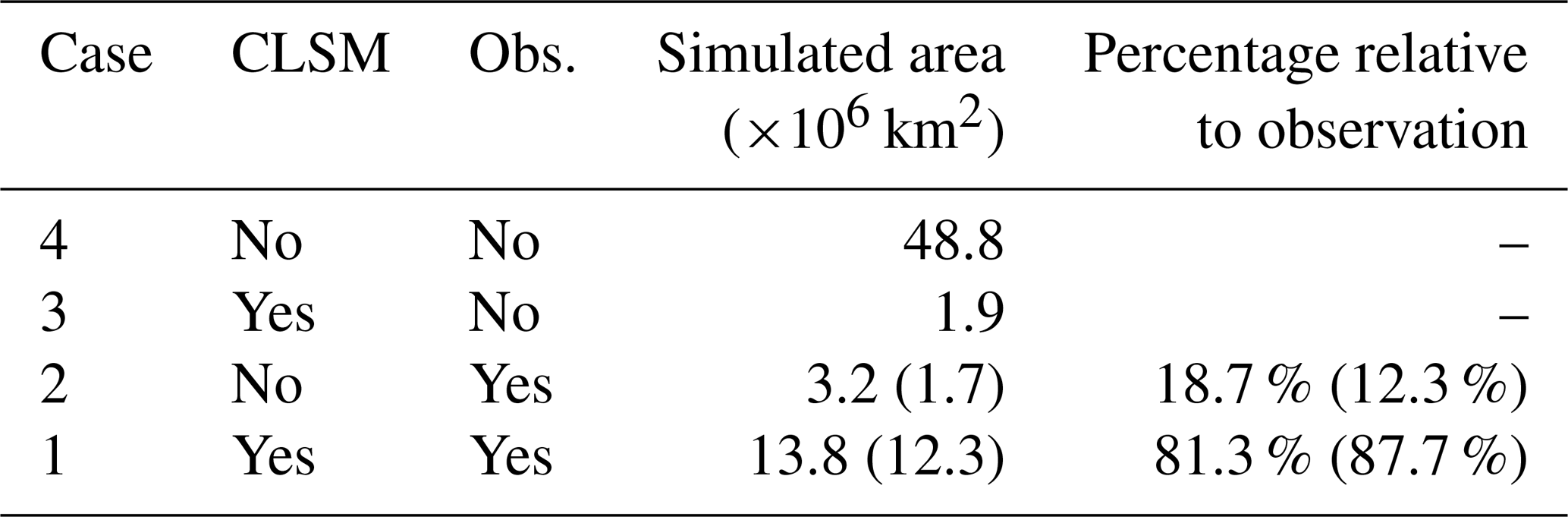
The disagreements between the simulated and observed permafrost extents (covering about a few degrees latitude) toward the south in Fig. 10a (green and blue areas at the southern edge of permafrost regions) are less of a concern, since the comparison in such areas is muddied by the interpretation of isolated permafrost in the observational map (Fig. 1b). The specific areas of each type shown in Fig. 10a are listed in Table 4. The simulated permafrost extent covers 81.3 % of the observation-based area (i.e. the total area of continuous, discontinuous, and sporadic permafrost regions) and misses 18.7 % of the observed permafrost area. When comparing simulated permafrost extent with only continuous and discontinuous types, these metrics change to 87.7 % and 12.3 %, respectively. Meanwhile, the permafrost extent is overestimated by 3.2 × 10⁶ km².

Table 4 Evaluation results for simulated permafrost extent against the permafrost map by Brown et al. (2002). The calculation was based on the comparison between simulated permafrost area and the total area of continuous, discontinuous, and sporadic permafrost regions from Brown's map. The number in the brackets was calculated against the total area of continuous and discontinuous permafrost regions.

To produce Fig. 10b, multi-year averages of CLSM-simulated ALT values were spatially averaged over each of the four permafrost types outlined in Fig. 1b. (As is appropriate, permafrost is only occasionally simulated over the fourth, isolated, permafrost type. The ALT average shown for this type is thus based on a particularly limited number of grid cells.) The average ALT is smallest in the continuous permafrost zone, higher in the discontinuous zone, and higher still in the sporadic permafrost zone; it is highest in areas of isolated permafrost. The progression, of course, is in qualitative agreement with expectations – larger breaks in permafrost coverage imply a greater amount of available energy, which should also act to increase ALT.

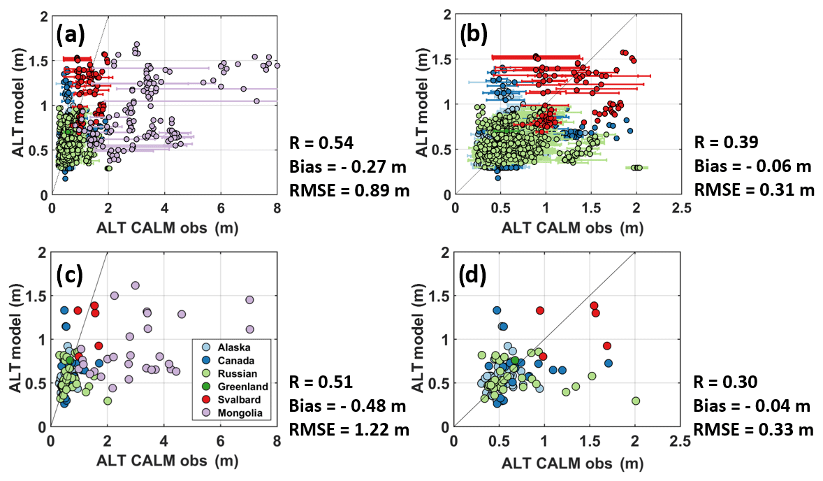
Figure 11 (a) Annual ALT from CLSM simulation vs. CALM observations with horizontal error bars indicating standard deviations of measurements within the model grid cell. Error bar is absent if the number of measurements within a 81 km² grid cell is less than three. (b) As in panel (a) but excluding the Mongolia sites. (c) The 38-year average ALT for the period 1980–2017 from CLSM simulation vs. CALM observations. (d) As in panel (c) but without the Mongolia sites. The correlation coefficient (R), bias, and root mean square error (RMSE) are provided next to each subplot.

The observed and CLSM-simulated annual ALT and multi-year ALT averages are compared in Fig. 11. Generally, the simulated annual ALT and the averages agree reasonably well with observations for shallow permafrost regions, that is, for smaller ALT. A large bias, however, is found for most of the Mongolia sites; in Mongolia, the observed annual ALT and the climatological ALTs tend to be much larger than the simulated ALTs (light purple dots in Fig. 11). Overall, the RMSE, bias, and R are all significantly improved when the Mongolian sites are excluded from consideration. Specifically for the climatological ALTs, the RMSE (and bias) of simulated ALT climatological means is 1.22 m (and −0.48 m), and it drops to 0.33 m (and −0.04 m) if the Mongolia sites are excluded (Fig. 11d). Given simplifications in the model, uncertainties in boundary conditions (e.g. vegetation types and soil properties), and upscaling issues stemming from the coarse-scale nature of the forcing data relative to the point-scale and plot-scale nature of the observations (i.e. the representative errors as indicated by the large standard deviation shown in Fig. 11a), these results seem encouraging. The correlation coefficient metric (R), however, is somewhat less encouraging, amounting to only 0.5 when considering all sites. The correlation coefficient is in fact lower (0.3) when the Mongolian sites are excluded; the correlation coefficient is 0.39 for the Mongolian sites considered in isolation. Note that the existing literature on simulated ALT fields (e.g. Dankers et al., 2011; Lawrence et al., 2012; Guo et al., 2017) reveals a general tendency for models to overestimate ALT climatology at the global scale. In light of this, our results suggest that the CLSM-simulated ALT fields are perhaps among the better simulation products, especially for shallow permafrost.

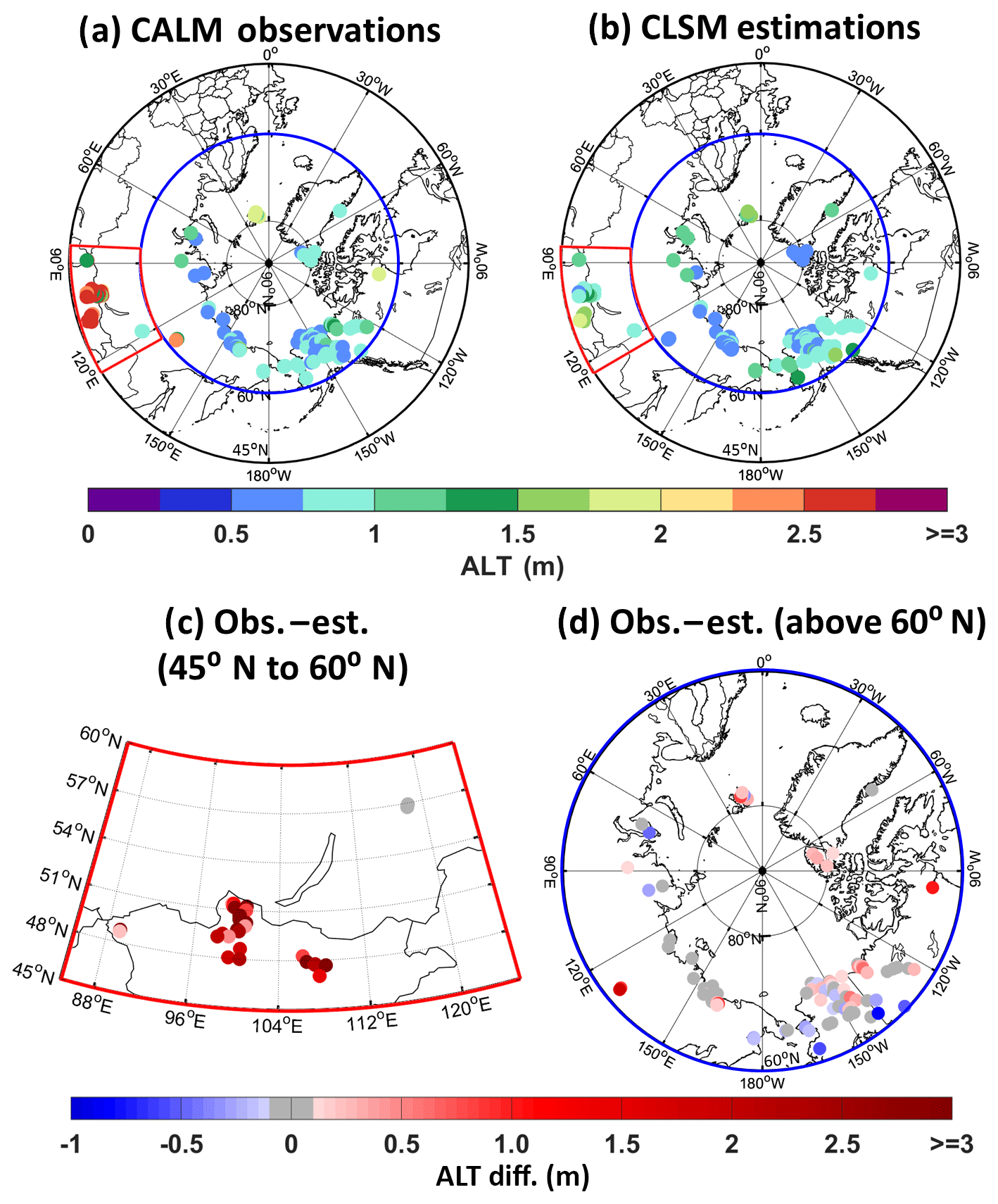
Figure 12 Multi-year average ALT at CALM site locations for (a) CALM observations and (b) CLSM results. (c) ALT difference between observations and model results for locations within 45–60^∘ N latitude and 85–125^∘ E longitude. (d) Same as panel (c) but for locations poleward of 60^∘ N latitude. In panels (c) and (d) grey indicates absolute ALT differences less than 0.10 m.

Comparing the observed and simulated spatial distributions of the ALT averages provides a further test of the accuracy of the simulation results (as shown in Fig. 12). The model successfully simulates the large-scale spatial patterns in ALT, capturing, for example, the variations in Siberia, Svalbard, northern Canada, and northern Alaska (see Fig. 12a, b). Figure 12c and d show the differences between the observed and estimated values in middle latitudes (45 to 60^∘ N) and high latitudes (60 to 90^∘ N), respectively; in agreement with Fig. 11a, the model clearly performs better in high-latitude regions, i.e. outside of Mongolia. Many of the sites north of 60^∘ N (Fig. 12d) are coloured grey, indicating a small error in the simulation of ALT at these sites – the errors at these sites range from only −0.10 to 0.10 m.

The significant underestimation of ALT in Mongolia might result from errors in the meteorological forcing provided by MERRA-2. However, a comparison (not shown) of MERRA-2 air temperatures with measurements at six weather stations collocated with CALM sites in Mongolia calls this explanation into question. While MERRA-2 summer temperatures are indeed too low at four of the weather stations examined, they are too high at the other two weather stations. An additional reason for the underestimation of ALT in Mongolia might be a mismatch between the land surface parameter values used in the model and the actual conditions at each site. For instance, detailed soil information (https://www2.gwu.edu/~calm/data/webforms/mg_f.html, last access: 27 July 2019) indicates that some Mongolian sites have special rocky soil types including limestones (e.g. M04), slatestones (e.g. M05), and gravelly sand (e.g. M06 and M08) that are not well represented in the model. As another example, sites on south-facing slopes presumably have much deeper ALT than those on slopes with less exposure to the sun, which is not captured by CLSM. The large representative errors of Mongolian sites are clearly illustrated by the standard deviation (although computed only with three to five measurements) as shown by the error bars in Fig. 11a.

5 Conclusion and discussion

We produced a dataset (effectively a derivative of MERRA-2) of permafrost variations in space and time across middle-to-high latitudes. This dataset can be considered unique in terms of its daily temporal resolution combined with a relatively high spatial resolution at the global scale (i.e. 81 km²). The dataset, which is derived from a state-of-the-art reanalysis (MERRA-2), shows reasonable skill in capturing permafrost extent (87.7 % of the total area of continuous and discontinuous types, according to one validation dataset) and in adequately estimating ALT climatology (with a RMSE of 0.33 m and a mean bias of −0.04 m), excluding Mongolian sites. We note that our MERRA-2-driven permafrost simulation results, while potentially better than those we might have obtained with MERRA forcing, are still lacking (e.g. in western Siberia). Still, with its resolution and available variables (ALT, subsurface temperature, and ice content at different depths), the dataset could prove valuable to many future permafrost analyses.

This work also provides a first comparison between two highly complementary approaches to estimating permafrost: model simulation and remote sensing. In northern Alaska, excluding sites that have ALT measurements exceeding the radar sensing depth (∼60 cm), the evaluation metrics for ALT retrievals against in situ measurements are better than those for simulated ALT at the 81 km² scale. However, the remotely sensed ALT estimates generally show lower levels of spatial variability relative to the simulated ALT estimates (and relative to the in situ observations), and the spatial patterns of the simulated and retrieved values differ considerably. The remote sensing approach is still relatively new, with many aspects still requiring development. It is important, though, to begin considering the modelling and remote sensing approaches side by side, as both should play important roles in permafrost quantification in the years to come. Indeed, once the science fully develops, joint use of modelling and remote sensing (e.g. through the application of downscaling methods) should allow the generation of more accurate permafrost products at higher resolutions.

It is important to note that the retrieved ALT was determined by the dielectric transition from thawed to frozen conditions, whereas the modelled ALT and the ALT for some of the in situ measurements was based on a freezing temperature of 0 ^∘C (see Sect. 2.1 and 2.3). Depending on local conditions, soil does not typically freeze at 0 ^∘C but rather at slightly lower temperatures (e.g. around −1 ^∘C) due to the presence of dissolved compounds that depress the freezing point (Watanabe and Wake, 2009). The sharp drop in conductivity and dielectric constant is much more accurately tied to a frozen state than to a temperature threshold. These and other differences in the various ALT measurement methods (Sect. 2.3) introduce considerable uncertainty into our comparisons. The use of the 0 ^∘C degree threshold in CLSM for determining the thawed or frozen layer may explain in part the model's underestimation of ALT, as may the lack of an explicit treatment of local aspect, errors in assigned model parameters, and so on.

Analysis of the CLSM-simulated data, along with data produced in idealized experiments with specific homogenized controls, shows how the statistics of permafrost variability in space are controlled by forcing variability and by variability in the imposed surface boundary conditions. In the idealized experiments, we employ successive homogenization of controls to quantify how meteorological forcing, soil type, and vegetation cover affect the underground thermodynamic processes associated with the variability of ALT along the AirMOSS flight paths in Alaska. Meteorological forcing and soil type are found to be the two dominant factors controlling ALT variability along these transects. Vegetation plays a smaller role by modulating the accumulation of snow. A multiple regression analysis relating yearly ALT jointly to accumulated air temperature and maximum SWE shows that time variations in these two latter quantities explain most of the time variability of ALT in the CLSM-identified permafrost regions.

Many aspects of the modelling framework may contribute to the noted errors in the simulated ALTs. For example, the observed climatological ALTs at the Mongolia sites are all larger than 3 m. This depth falls well within the sixth soil layer of the model, which has a thickness of 10m; the subsurface vertical resolution in the CLSM may be too coarse to capture these deeper ALTs. Test simulations (not shown) with alternative model configurations indicate that increasing the number of soil layers may act to decrease somewhat the simulated ALT, suggesting that our values may be a little overestimated; however, based on results from a new study by Sapriza-Azuri et al. (2018), our use of a no-heat-flux condition at the bottom boundary rather than a dynamic geothermal flux may lead to underestimates of ALT. Such uncertainties should naturally be kept in mind when interpreting our results. Our supplemental simulations (not shown) also suggest that increasing the total modelled soil depth has only a small impact on simulated ALT. Uncertainty in our description of soil organic carbon, i.e. both soil carbon content and vertical carbon distribution, leads to corresponding uncertainty in our ALT simulations. We indeed find a significant improvement in simulated ALT at several Mongolian sites when we arbitrarily impose less total soil carbon content and concentrate less soil carbon in top layers (not shown). Besides the vertical distribution of soil carbon, the vertical variation in other soil hydrological properties (e.g. soil texture and porosity) should also play a significant role since they all affect soil thermal conductivity and heat capacity. In addition, the lack of a necessary organic layer on top of soil column and the related thermal processes is also a major deficiency for the model, especially in ecosystem-protected permafrost regions.

Another issue affecting our ALT comparisons is the climatological representation of vegetation parameters such as LAI used in CLSM. An additional investigation (not shown) revealed large differences between the LAI climatology used in CLSM and more realistic, time-varying, satellite-based LAI products at several Mongolian sites. In addition, while we did exclude from our analyses any measurements that were affected by notable disturbance (e.g. wildfire), the impacts of other potential land changes on ALT, including overgrazing in Mongolia (Sharkhuu and Sharkhuu, 2012; Liu et al., 2013), were not explicitly treated in the model. The model also lacks the vertical advective transport of heat in the subsurface due to downward-flowing liquid water, which can significantly affect permafrost thawing (Kane et al., 2001; Rowland et al., 2011; Kurylyk et al., 2014). Also relevant are potential errors in the MERRA-2 forcing. The MERRA-2 reanalysis is known to have problems capturing trends in high latitudes (Simmons et al., 2017).

Such modelling deficiencies must always be kept in mind when evaluating a product like the one examined here. That said, as long as appropriate caution is employed, the product could have significant value for further analyses of permafrost. The product features daily subsurface temperatures and depth-to-freezing estimates over middle-to-high latitudes in the Northern Hemisphere at an 81 km² resolution, covering the period 1980–2017. It is, in a sense, a value-added derivative product of the MERRA-2 reanalysis and will be available via the National Snow and Ice Data Center (NSIDC). The comparisons against observations discussed above, along with the intuitively sensible connections shown between permafrost variability, forcing variability, and boundary condition variability, give confidence that this dataset contains useful information. These data can potentially contribute, for example, to ecological studies focused on the dynamics of microbial activity and soil respiration in cold regions, on vegetation migration/adaptation in response to climate change, and so on.