Improving gridded snow water equivalent products in British Columbia, Canada: multi-source data fusion by neural network models

Estimates of surface snow water equivalent (SWE) in mixed alpine environments with seasonal melts are particularly difficult in areas of high vegetation density, topographic relief, and snow accumulations. These three confounding factors dominate much of the province of British Columbia (BC), Canada. An artificial neural network (ANN) was created using as predictors six gridded SWE products previously evaluated for BC. Relevant spatiotemporal covariates were also included as predictors, and observations from manual snow surveys at stations located throughout BC were used as target data. Mean absolute errors (MAEs) and interannual correlations for April surveys were found using cross-validation. The ANN using the three best-performing SWE products (ANN3) had the lowest mean station MAE across the province. ANN3 outperformed each product as well as product means and multiple linear regression (MLR) models in all of BC's five physiographic regions except for the BC Plains. Subsequent comparisons with predictions generated by the Variable Infiltration Capacity (VIC) hydrologic model found ANN3 to better estimate SWE over the VIC domain and within most regions. The superior performance of ANN3 over the individual products, product means, MLR, and VIC was found to be statistically significant across the province.

1 Introduction

In areas of the world with significant alpine regions, many drainage basins exhibit a predominantly nival regime. Under such conditions, which are characteristic of the province of British Columbia (BC), Canada, accurate snow water equivalent (SWE) estimation is particularly crucial for water supply, hydropower generation, and flood forecasting and planning purposes. The ability of current methods and products to give accurate SWE estimates is limited by a number of topographic and climate factors. Forest cover, topography, and large SWE accumulations pose challenges for physical models containing multiple simplifications and parameterizations, as well as for satellite-based products, which can experience signal masking and wash-out (Chang et al., 1996; Derksen, 2008). Likewise, reanalysis and assimilation-based products are susceptible to biases arising from various structural limitations (e.g., elevation biases tied to spatial resolution) and uncertainties in the climate mean state (Dutra et al., 2011; Reichler and Kim, 2008). Mudryk et al. (2015) compared various gridded products across the Northern Hemisphere and observed large spreads in SWE with magnitudes on the order of the SWE interannual variability. These spreads were seen particularly in alpine regions with complex topography and in the Arctic, a region of large data gaps. A similar set of gridded products was examined and ranked by Snauffer et al. (2016) over the rugged, forested topography of British Columbia. Product correlations, biases, and MAEs were determined by comparison with in situ manual snow surveys and reported by survey month and physiographic region. While the best products were generally superior performers across the determined statistics and the majority of regions, all products were found to underestimate SWE and imperfectly represent interannual fluctuations, particularly in the regions of highest snow accumulation. Against this backdrop, the current work set out to improve the accuracy of SWE estimates in the same topographically complex region by combining an ensemble of products with relevant site covariates utilizing a data fusion approach.

Numerous models and estimation techniques have attempted to better characterize SWE. Nascent satellite-based efforts involved the use of multiple linear regression (MLR) to retrieve snow parameters from passive microwave data. Though newer platforms have become available, many of the early algorithms (Chang et al., 1987; Foster et al., 1997; Tait, 1998) rely on the Defense Meteorological Satellite Program (DMSP) Special Sensor Microwave/Imager (SSM/I) brightness temperature data, which constitute a long passive microwave record covering July 1987 to December 2015 derived from intercalibrated measurements across several spaceborne platforms (Wentz, 2013). While the early linear approaches performed well in areas of low snow accumulation, forest cover, and topographic relief, mountainous regions with dense vegetation and deep snowpacks were not as well represented.

Machine learning methods began to become an important tool in the environmental sciences in the 1990s and have since spread to many application areas (Hsieh, 2009). Early applications of machine learning methods for retrieving SWE were developed by Chen et al. (2001) and Guo et al. (2003) using artificial neural networks (ANNs). Inputs were based on a snow hydrology model, and outputs derived from a dense media radiative transfer model were iteratively computed until the ANN results converged on observations. The model improved on previous efforts by improving grain size representation and applying a spatially distributed snow accumulation and melt model. Tedesco et al. (2004) compared SWE retrieved from an ANN to values from the spectral polarization difference (SPD) algorithm (Aschbacher, 1989), the Helsinki University of Technology (HUT) snow emission model (Pulliainen et al., 1999), and the Chang algorithm (Chang et al., 1987; Foster et al., 1997). The ANN used SSM/I 19 and 37 GHz vertical and horizontal brightness temperatures as inputs and the national operational snow observations of the Finnish Environment Institute or HUT simulated brightness temperatures as the target data. Under dry snow conditions enforced by only considering days on which the maximum temperature was lower than −5 ^∘C, the ANN outperformed these other methods when trained with observations. Evora et al. (2008) developed a data fusion modeling framework utilizing ANNs, passive microwave data, and geostatistics. Predictors for this framework were seven passive microwave channels and the interpolated minimum temperature. The target SWE field was derived from snow depth and density measured manually at snow stations and interpolated by a kriging with external drift (KED) algorithm using elevation as the secondary variable. More recently Tong et al. (2010) compared SWE predictions of ANNs using microwave brightness temperatures (TBs) to those of the SPD algorithm Aschbacher (1989) and other TB difference algorithms (Chang et al., 1987; Derksen, 2008) in the Quesnel River Basin of BC, finding that ANNs which included the most TB channels outperformed other networks and algorithms. Binaghi et al. (2013) applied radial basis function networks to estimate snow cover thickness in the Italian Central Alps, finding that this approach outperformed inverse distance weight and spline interpolation methods commonly used in similar contexts with limited numbers of homogeneously distributed measurement sites. These and other studies covered in various review papers (Evora and Coulibaly, 2009; Gan, 1996; Shi et al., 2016) demonstrate the promise of more accurate snow estimates via machine learning methods, but they do not incorporate existing SWE products directly.

Manual snow surveys, taken on courses extending tens of meters, cannot be accurately represented by large-scale gridded products with resolutions on the order of tens of kilometers (Mudryk et al., 2015). Inherent SWE differences can be introduced by disparities between mean grid cell elevation and station elevation, as well as other topographic controls. Even higher-resolution covariates such as the GLOBE 1 km DEM (Hastings et al., 1999) still fail to adequately reflect important physical contexts at survey sites (e.g., local slope and aspect) which can significantly affect measured values. In spite of the scale mismatch, the combination of large-scale gridded products with covariates such as finer terrain information and physiographic context may capture the spatiotemporal patterns in the manual snow surveys. Scale issues are further addressed in Sect. 3.2.

The objective of this work is to apply data fusion techniques to readily available gridded SWE products, manual snow surveys, and covariates in order to better estimate SWE in BC. Means of six products are evaluated, as are means of the best three of these products based on previous rankings (Snauffer et al., 2016). Relevant covariates are further combined with these sets of products in MLR models as well as nonlinear ANNs. The assumptions and limitations underlying this approach are discussed in detail in Sect. 3.2.

2 Study area

The study area, namely the province of BC, can be separated into five physiographic regions, which are shown in Fig. 1. These regions vary considerably in terms of their topography and climate, as well as the amount of snow they receive, as reported in Snauffer et al. (2016). Along the entire western edge of BC, the Coast Mountains and Islands region is a highly rugged series of mountain ranges and troughs with a mean station SWE of 782 mm in April. The Columbia Mountains and Southern Rockies region to the southeast is also very rugged with high mean elevation and an average April SWE of 565 mm. Possessing a more moderate 337 mm mean SWE as measured during April surveys, the Northern and Central Plateaus and Mountains region is relatively flat along the plateaus in the north and has low mountain ranges scattered throughout. The Interior Plateau region in the middle of the province is mostly flat except in the east and has a similarly moderate April mean station SWE of 283 mm. To the northeast of the province, the region of the Great Plains of British Columbia, referred to in this work as the “BC Plains”, has the lowest relief and SWE accumulations, reporting a station average of 88 mm SWE in April. Further descriptions of the study area are detailed by British Columbia Ministry of Forests (1995) and Holland (1964).

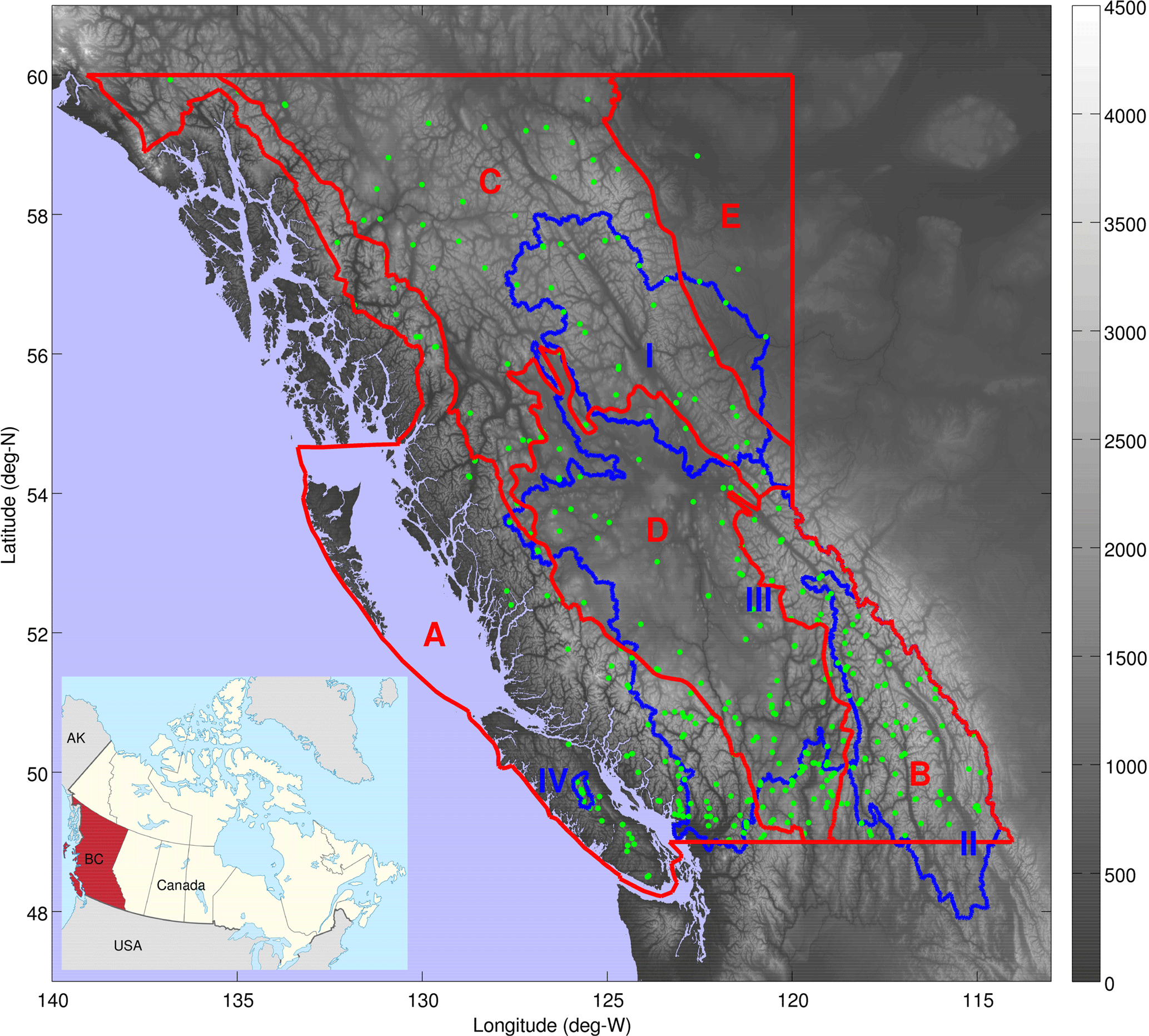
Figure 1 Physiographic regions of British Columbia, Canada, overlaid on the GLOBE 1 km DEM. Elevations are shown according to the legend with units of meters above sea level. The five physiographic regions are outlined in red: (A) Coast Mountains and Islands, (B) Columbia Mountains and Southern Rockies, (C) Northern and Central Plateaus and Mountains, (D) Interior Plateau, and (E) BC Plains. SWE accumulations generally increase from region A to region E. Outlined in blue is the VIC domain run by the Pacific Climate Impacts Consortium, covering four basins throughout BC: (I) the Peace, (II) upper Columbia, (III) Fraser, and (IV) Campbell River watersheds. Manual snow survey station locations are indicated by green dots. Inset: a map of Canada (source: Wikimedia Commons) shows BC highlighted in red. The province is bordered to the south by the contiguous United States (USA) and to the west by the US state of Alaska (AK).

3 Methods

Various publicly available SWE data sets have global to hemispheric coverage and can provide information on snow spatiotemporal distribution over BC. This study considered four reanalysis products (ERA-Interim; ERA-Interim/Land, hereinafter identified as “ERALand”; MERRA; and MERRALand), a land data assimilation system (GLDAS2), and an observation-based product (GlobSnow). Key predictors of snow distribution and evolution are these gridded SWE products, and the target data are manual snow surveys conducted throughout the province.

3.1 Input data

The following gridded SWE products were used as predictors in this study and are described in further detail in Snauffer et al. (2016). ERA-Interim (Dee et al., 2011), a reanalysis product of the European Centre for Medium-Range Weather Forecasts (ECMWF), assimilates land surface, oceanographic, atmospheric, and spaceborne measurements from numerous sources using the Integrated Forecast System (IFS) at T255 spectral (∼80 km) horizontal resolution. ERA-Interim/Land (Balsamo et al., 2015) is an offline rerun of ERA-Interim using an improved land surface model known as HTESSEL (Hydrology-Tiled ECMWF Scheme for Surface Exchanges over Land) and precipitation adjustments based on the Global Precipitation Climatology Project (GPCP) v2.1. The Modern-Era Retrospective analysis for Research and Applications, or MERRA (Rienecker et al., 2011), ingests a host of land, oceanic, and atmospheric data using the Goddard Earth Observing System Data Assimilation System Version 5 (GEOS-5) at a resolution of one-half degree latitude by two-thirds degree longitude. MERRALand (Reichle et al., 2011) is an offline land surface simulation based on MERRA which uses the land surface model Fortuna-2.5 and makes precipitation adjustments based on the NOAA Climate Prediction Center “Unified” (CPCU) product. The Global Land Data Assimilation System Version 2, known as GLDAS-2 (Rodell et al., 2004) and produced by NASA, runs forcings from the Princeton meteorological data set (Sheffield et al., 2006) on one of four land surface models, including the 0.25^∘ Noah implementation that is used in this study. GlobSnow (Takala et al., 2011), the “mountains unmasked” data set provided by the Finnish Meteorological Institute (FMI), relies on a background field of snow depths created using synoptic observations and a forward model of satellite-based microwave radiometer measurements to construct a 25 km horizontal resolution SWE field. Other evaluated products in Snauffer et al. (2016), GLDAS-1 and CMC, do not cover the early part of the study period (1980–2010) and hence are not included in this work.

The target data are manual snow surveys (MSSs) conducted by the Snow Survey Network Program for the BC River Forecast Centre (Ministry of Environment and Climate Change Strategy, 2015). At each designated survey site a column of snow is extracted using a standard Federal snow sampler and weighed to determine SWE. The mean of SWE measurements at 5 to 10 points along a snow course is calculated to find the station areal average, which is then reported. Surveys are taken up to eight times a year, once at the beginning of months January through June and once mid-month in May and June, and they are currently conducted at 167 stations throughout the province with another 216 stations with historical but no current measurements. Sampling frequencies and temporal ranges vary considerably by station, with some records dating back to 1935.

Automated snow pillow data were also examined as a part of this work. These data were found to be considerably more prone to obvious errors than the manual snow surveys. Such errors included negative values, snow accumulation and melt curves that contained sudden jumps, drops and unrecognizable noise, missing values that were sometimes interpolated, and other problems. In addition to passing such errors into the model, the likelihood exists to introduce redundancy, as many of the snow pillows are co-located with manual snow survey sites. Consequently, only the manual snow surveys were used as target data.

3.2 Artificial neural network construction

An ensemble ANN (hereafter ANN) was constructed following Cannon and McKendry (2002) using the implementation by Cannon (2015). ANN topology consisted of an input layer, one hidden layer, and an output later with a single node for SWE. A single hidden layer is adequate to model any nonlinear continuous function (Hsieh, 2009). The hyperbolic tangent sigmoid function was used as the hidden layer activation function, the identity function was used for the output layer, and predictor and predictand variables were standardized (zero mean and unit standard deviation) prior to model training. Initial model weights were set randomly in the range of $\pm \sqrt{\mathrm{0.8}/d_{\mathrm{in}}}$, where d_in is the number of inputs (Thimm and Fiesler, 1997). The optimization function employed was the Broyden–Fletcher–Goldfarb–Shanno method or “BFGS method” (Fletcher, 1970; Nash, 1979). Training data sets for the individual ANN ensemble members were created using the block bootstrap (Davison and Hinkley, 1997), with each block made up of all training cases for a given station. To prevent overfitting, early stopping was used to regularize individual ensemble members; ANN training was stopped when validation error, as monitored on the out-of-bootstrap cases, reached a minimum. The optimal number of hidden nodes for each test split was determined by minimizing the ensemble's out-of-bootstrap RMSE over the training data. Following model selection and training, predictions from the 50 ensemble members were averaged for each test split, and statistics for each test split station were calculated accordingly.

In total, manual snow survey data from 386 stations across BC were available for training and testing. Of those stations 256 had at least 10 years of measurements within the overlapping period of record of the six gridded products (1980–2010). This was considered to be an adequate length to generate representative statistics for testing the ANN by cross-validation. Ten test splits were created by selecting every tenth station, stratified by watershed, such that for each split one-tenth of the stations were excluded from training. The result was an approximately uniform spread of test stations throughout the province in each split, as shown in Fig. 2 (green dots). Inevitably there were large areas with little in situ data, particularly along the coast and in the BC Plains to the north, but the use of all available data outside the test split maximized the spatial coverage of the training set. The MAE and April survey correlation reported at each station were computed using predictions from the ANN which did not include data from that station in its training set.

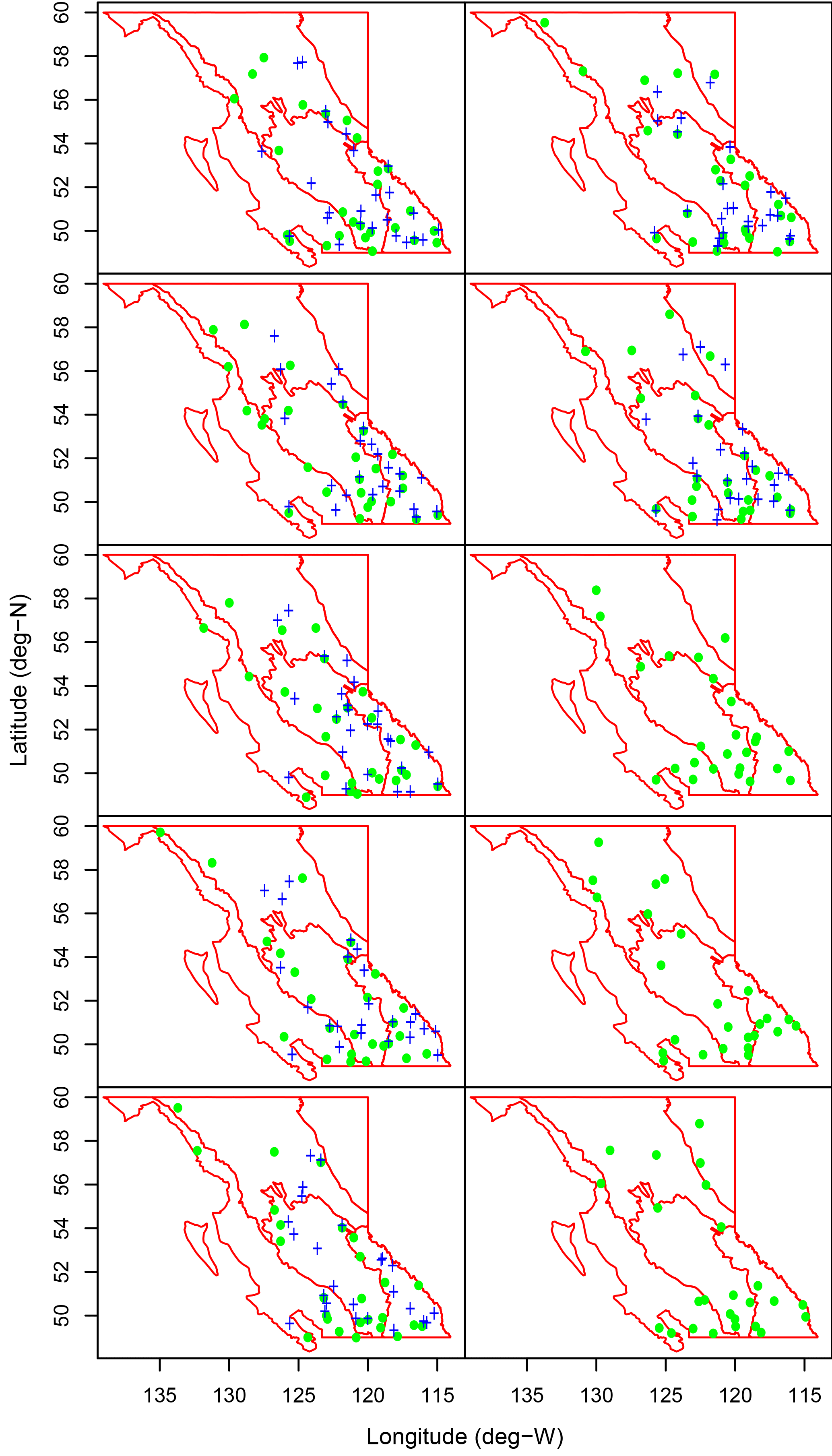
Figure 2 MSS station locations used in evaluating combination products. Green dots show the distribution of 10 test splits for comparing means, MLRs, and ANNs to gridded SWE products throughout BC by cross-validation. Blue crosses show the distribution of seven test splits for comparing ANNs to VIC runs in four BC watersheds. Physiographic regions are outlined in red.

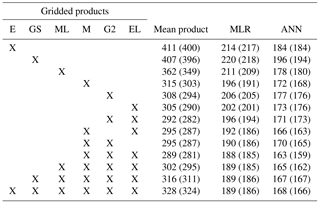
Table 1 Mean station MAEs (in mm SWE) for individual and combinations of products and corresponding MLR and ANN runs, with the mean station MAEs computed using only the VIC stations given in parenthesis. Products shown are ERA-Interim (E), GlobSnow (GS), MERRALand (ML), MERRA (M), GLDAS2 (G2), and ERALand (EL).

Due to their coarse spatial resolution, the gridded products tend to capture broad spatiotemporal SWE patterns over BC, but values still exhibit large biases with respect to MSS observations (Snauffer et al., 2016). In addition to the gridded SWE products, the following base set of predictors were included in the model: elevation, elevation bias, latitude, longitude, physiographic region, year, and sine and cosine of 2π times the elapsed year fraction. These predictors represented major spatial and temporal dimensions to the ANN training, as well as broad location context information (e.g., physiographic region). Predictor screening was not necessary because relatively few base covariates were identified, and correlations between predictors would not diminish model performance. Station elevation biases were calculated as the grid cell mean elevations found from the GLOBE 1 km DEM (Hastings et al., 1999) minus the reported station elevations, and elevation biases corresponding to each included product were used as predictors. Physiographic regions were represented in the model using discrete logical variables for each region, so-called 1-of-c coding as described in Bishop (1995). These predictors provide specific spatial and temporal information as well as broad location context information.

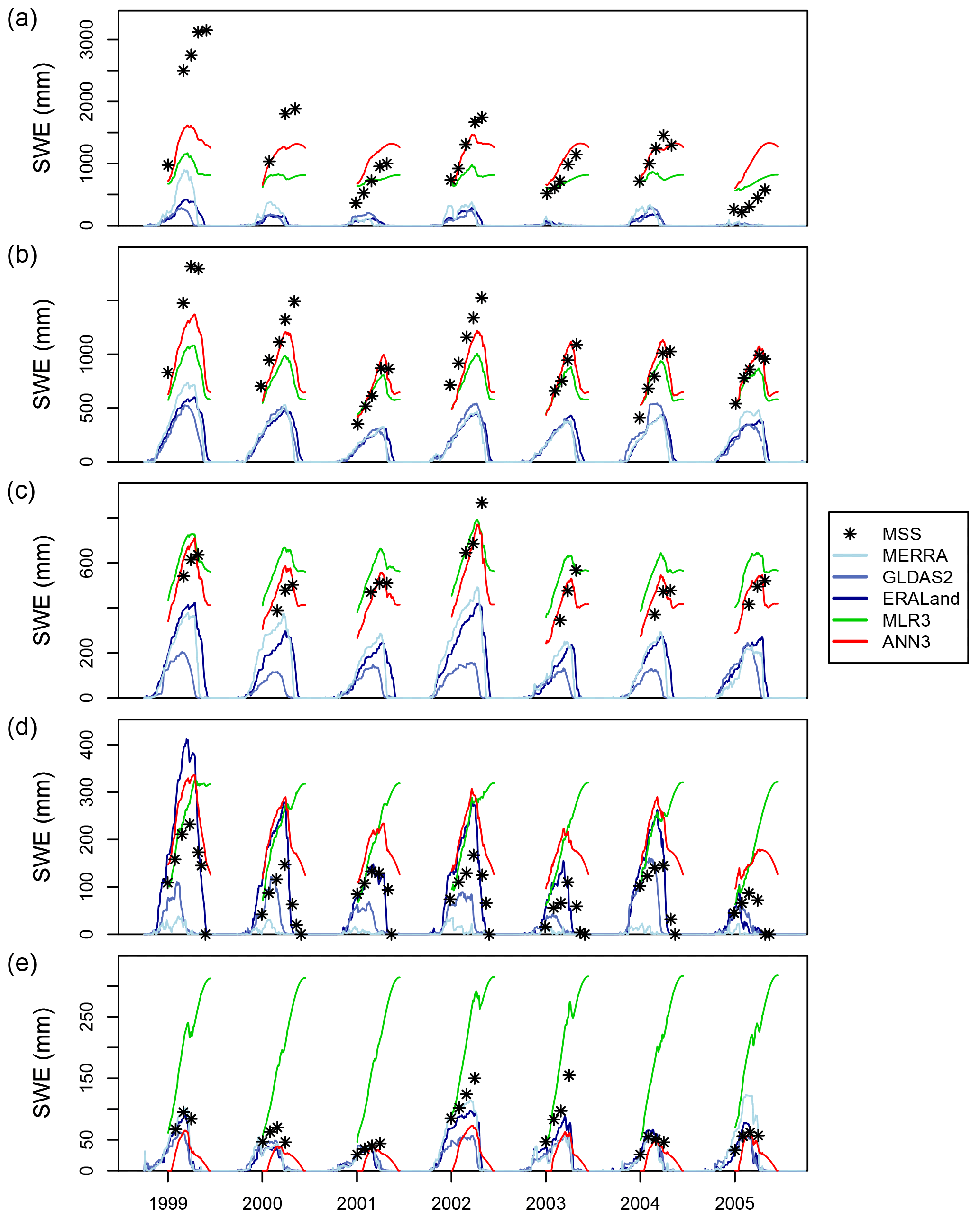
Figure 3 SWE time series for manual snow survey stations, the best three gridded SWE products, MLR3, and ANN3. Gridded products are ordered by increasing overall performance, with darker blues for better-performing products. MLR3 and ANN3 estimates are masked outside the mean first and final survey dates (2 January and 15 June respectively). A representative station is shown for each of the five physiographic regions of BC: (a) station 1D08 Stave Lake in the Coast Mountains and Islands, (b) station 2A25 Kirbyville Lake in the Columbia Mountains and Southern Rockies, (c) station 4B08 Mount Cronin in the Northern and Central Plateaus and Mountains, (d) station 2F11 Isintok Lake in the Interior Plateau, and (e) station 4C05 Fort Nelson Airport in the BC Plains.

Figure 4 Mean station MAE for several SWE products/combinations for regions of BC in order of descending mean accumulations: (a) Coast Mountains and Islands, (b) Columbia Mountains and Southern Rockies, (c) Northern Plateaus and Mountains, (d) Interior Plateau, (e) BC Plains, and (f) province-wide (combining all data from the five preceding panels). Shown are MAEs with 95 % confidence intervals based on n=5000 bootstrap samples for the six gridded products in blue: ERA-Interim (E), GlobSnow (GS), MERRALand (ML), MERRA (M), GLDAS2 (G2), and ERALand (EL). Dark blue indicates three best-performing products. Also shown are three fusion techniques (mean, MLR, and ANN) using all six products (green) and the three best-performing products (brown). Note the vertical scale in panels (a) and (b) is double that of panels (c) through (f).

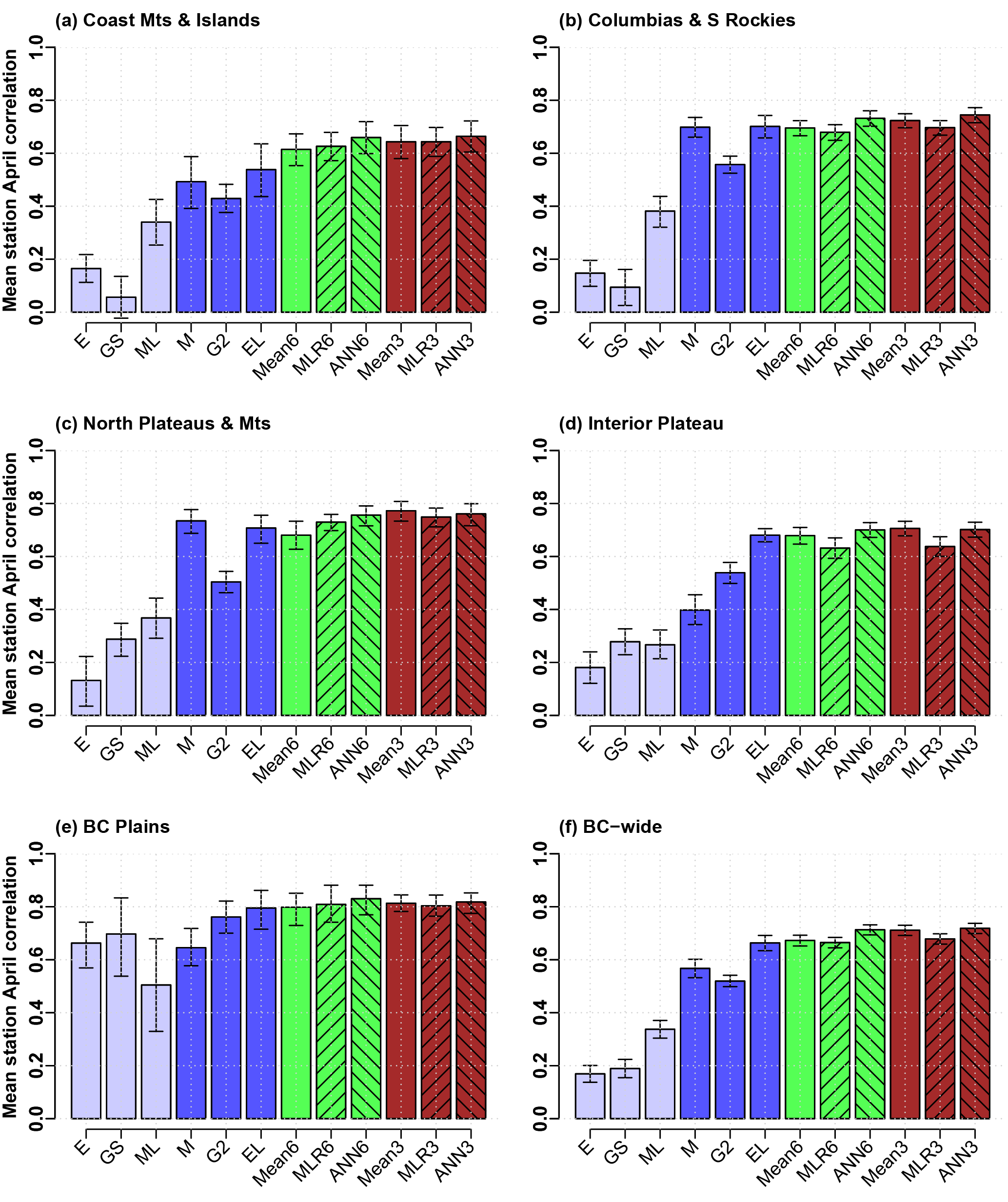
Figure 5 Mean station April correlation for several SWE products/combinations for regions of BC in order of descending mean accumulations: (a) Coast Mountains and Islands, (b) Columbia Mountains and Southern Rockies, (c) Northern Plateaus and Mountains, (d) Interior Plateau, (e) BC Plains, and (f) province-wide. Product and combination abbreviations and colors are as in Fig. 4.

From a temporal perspective, the most important predictor of seasonal SWE is the fraction of the year elapsed at the time of observation. This elapsed year fraction is modeled using trigonometric predictors (sine and cosine) as it is a periodic signal. The stationarity of each utilized data set was not evaluated in the course of this study. In order to handle the prospect of non-stationary data, linear or otherwise, the value of the observation year was included as a predictor, allowing the ANN to account for changes in the joint probability distribution over time.

The assumptions underlying this approach include that the SWE field can be reliably resolved by an ANN topology that includes a single hidden layer, which is suitable for modeling any nonlinear continuous function (Hsieh, 2009). Overfitting is assumed to be adequately mitigated using early stopping and an ensemble of 50 members. It is also implicitly assumed that enough predictors are employed to adequately cover the solution space, though the number of predictors is less important than the quality of those predictors. Outside the given study area and time window, SWE estimates are less reliable, as properly trained ANNs perform nonlinear interpolation well but extrapolate poorly, potentially leading to significant deviations from the true signal beyond the bounds of the predictor training space (Hsieh, 2009).

As previously mentioned, MSS values found at sites on the order of 10 m do not adequately represent SWE averaged across gridded product cells. Since elevation is a key indicator in both SWE accumulation and melt (Anderton et al., 2004), among the most apparent scale issues is the difference between survey site elevation and grid cell mean elevation. Including such elevation differences as predictors adds important site-specific context but also carries limitations in capturing interactions of topography and the atmosphere. Local elevation minima and maxima may be subject to wind redistribution from peaks to valleys depending on surrounding topography, and weather systems drop different amounts of snow on windward and leeward mountain slopes. Nevertheless, elevation and grid cell elevation differences may provide a basic indication of subgrid SWE variability. Another important piece of local context is location within the province, key covariates of which include latitude, longitude, and physiographic region.

Efforts to include additional local information were limited by lack of extensive site-specific metadata and appropriate regional scale representations. For instance, while various ground cover products are available, the actual site forest cover is highly dependent on snow course location, time since last maintenance, and other factors, which vary considerably across the MSS data set (Tony Litke, personal communication, 2016). As a result, only this base set of covariates has been employed. The main focus of this work, however, was to find which combination(s) of products lead to the best result. While other covariates may incrementally improve the ANN performance, use of this base covariate set should suffice for this purpose.

The gridded SWE product combinations shown in Table 1 were used as predictors in the ANNs. Multiple linear regression (MLR) models were run using the same sets of predictors and test station splits, and their results are listed alongside those of the ANN models for comparison of linear and nonlinear data fusion techniques. The predictor combinations included each gridded product run individually as well as in combination with better-performing products. In addition, each two-product combination of the three best products was run. The rationale for this approach was the desire to limit the total number of ANN runs to substantially less than all 63 possible combinations of any number of products, running those most likely to give performance insights and improvements. The three best-performing products had mean station MAEs across BC that were within 5 % of each other, whereas other products had mean station MAEs 15–30 % higher than the top product, ERALand. Furthermore, it was not anticipated, for instance, that adding the poorest-performing product to an ANN of the best three would outperform an ANN of the best four. Only observations for which all six gridded products had SWE values within 7 days of the observation date were used, so that all models were based on the same set of observations.

A number of alternative machine learning methods were investigated in the course of this work. Bayesian neural network (BNN) and support vector machine (SVM) runs were executed but did not result in notable improvements over the ANN in spite of additional computational cost. While studies (Forman and Reichle, 2015; Xue and Forman, 2015) have shown machine learning methods such as SVM to be superior over ANNs for snow-related parameters, Lima et al. (2015) found that in an evaluation of four different nonlinear methods across nine different environmental data sets, no single nonlinear method consistently outperformed the others. Though an exhaustive exploration of machine learning algorithms was not the objective of this manuscript, the machine learning runs completed indicated that, of the investigated algorithms, the ANN was at least comparable, if not superior, for this application and data sets.

Figure 6 Bootstrap mean station MAE differences between several SWE products/combinations and the reference (the mean of six products). First quartile, median, and third quartile are plotted respectively as the bottom, waist, and top of each box, and 95 % confidence intervals are indicated by whiskers. MAE difference spreads are shown for regions of BC in order of descending mean accumulations: (a) Coast Mountains and Islands, (b) Columbia Mountains and Southern Rockies, (c) Northern Plateaus and Mountains, (d) Interior Plateau, (e) BC Plains, and (f) province-wide. Product and combination abbreviations and colors are as in Fig. 4. Note differences in vertical scale.

Figure 7 Bootstrap mean station April correlation differences between several SWE products/combinations and the reference (the mean of six products). Quartiles and 95 % confidence intervals are shown for regions of BC in order of descending mean accumulations: (a) Coast Mountains and Islands, (b) Columbia Mountains and Southern Rockies, (c) Northern Plateaus and Mountains, (d) Interior Plateau, (e) BC Plains, and (f) province-wide. Product and combination abbreviations and colors are as in Fig. 4. Note differences in vertical scale.

3.3 Hydrologic model comparison

The Variable Infiltration Capacity (VIC) hydrologic model is used by the Pacific Climate Impacts Consortium (PCIC) to conduct hydrologic assessments for the province of British Columbia (Pacific Climate Impacts Consortium, 2014). VIC is a macroscale hydrologic model that solves full surface water and energy balances (Liang et al., 1994), sharing many basic features with land surface models (LSMs) in global climate models (GCMs). The land surface is modeled as a grid of large, flat, uniform cells, and sub-grid heterogeneity is handled via statistical distributions. The land–atmosphere fluxes and water and energy balances are simulated at a daily or sub-daily time step. Water can only enter a grid cell via the atmosphere, which means that water in the channel network stays in the channels and subsurface flow between grid cells is not included in the water balance. For the 1∕16^∘ grid cells used in the PCIC implementation, this is a reasonable approximation.

The PCIC VIC implementation currently covers four watersheds throughout BC (Pacific Climate Impacts Consortium, 2014), as shown in Fig. 1. Relevant model parameters, specifically snow/rain temperature thresholds and snow albedo decay curves, were explicitly adjusted to reproduce observed SWE at snow pillows, with subsequent automated multi-objective calibration to reproduce streamflow series and volume errors (Schnorbus et al., 2010). The model is forced with daily observations for minimum and maximum temperature, precipitation, and wind on a 1∕16^∘ grid (Schnorbus et al., 2014).

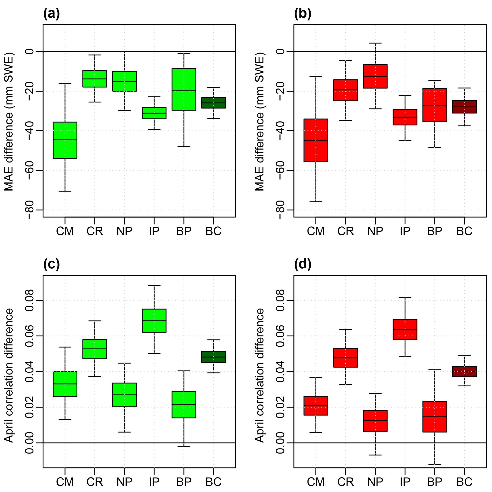
Figure 8 Box plots of bootstrap station differences in MAEs and April correlations showing quartiles and 95 % confidence intervals for ANNs of six products, ANN6 (green), and of the best three products, ANN3 (red), relative to MLR6 and MLR3 respectively. Bootstrap difference distributions are shown for (a) ANN6−MLR6 MAEs, (b) ANN3−MLR3 MAEs, (c) ANN6−MLR6 April correlations, and (d) ANN3−MLR3 April correlations. Shown are the differences for each physiographic region: Coast Mountains and Islands (CM), Columbia Mountains and Southern Rockies (CR), Northern and Central Plateaus and Mountains (NP), the Interior Plateau (IP), and the BC Plains (BP), as well as province-wide (BC).

Figure 9 Box plots of bootstrap station differences in MAEs and April correlations showing quartiles and 95 % confidence intervals for ANNs of six products, ANN6 (purple), and of the best three products, ANN3 (orange), with respect to VIC. Bootstrap difference distributions are shown for (a) ANN6−VIC MAEs, (b) ANN3−VIC MAEs, (c) ANN6−VIC April correlations, and (d) ANN3−VIC April correlations. Notation for the physiographic regions follows Fig. 8.

A second set of ANN runs was conducted using a subset of the test stations previously used. Only the MSS stations that were within the VIC domain and that had at least 10 years of measurements were used for testing. The 173 stations which met this criterion were divided into seven test splits of 24 or 25 stations each, ordered by watershed, such that for each split one-seventh of the VIC long record stations were excluded from training. This selection results in a relatively uniform spread of test stations for each split over the VIC domain as shown in Fig. 2 (blue crosses). Model training and MAE and correlation computation for each station were performed as in the full-province runs.

4 Results

Results of ANN runs for different combinations of products in this study are shown in Table 1. The gridded products used are listed in order of increasing performance across the entire province: ERA-Interim (E), GlobSnow (GS), MERRALand (ML), MERRA (M), GLDAS2 (G2), and ERALand (EL). Mean station MAEs are presented for single and average gridded product SWE values, plus MLRs and ANNs constructed using test splits of 256 stations across BC. Mean station biases were found to mirror mean station MAEs, as errors are largely the result of underestimates of SWE in most regions of the province (see the Supplement). MAEs are also shown for those same combinations based on test splits of 173 stations within the VIC domain. Using the individual products in an ANN with a base set of relevant spatiotemporal covariates improves the mean station MAE by 43 to 55 %. ANNs and MLRs based on combinations of the products further improve the mean station MAE, and MAEs for the ANNs are consistently lower than the corresponding values for the MLR models. While ANNs using multiple products all outperform those using single products, the best performance was achieved by a combination of the three best products: MERRA, ERALand, and GLDAS2. The differences in mean station MAE between the three-product ANN and ANNs that use more products are very small, suggesting that adding the products that do not perform as well does not bring additional useful information into the model. These results are consistent both for ANNs that use test splits of all 256 stations and for those that rely on test splits of the 173 VIC stations.

While comparing snow statistics aggregated across BC is useful for broad comparisons, SWE is a highly inhomogeneous field due to climatic and topographic variability in the province. Figure 3 illustrates the variability at stations across the five physiographic regions of the province. SWE values from manual snow surveys, gridded products, and combinations are plotted for representative stations, each of which has a station MAE close to the mean for the encompassing region. Regions are ordered by decreasing mean SWE accumulations in panels (a) through (e). The time interval shown covers snow seasons of 1999, a year of relatively high accumulations across the province, to 2005, a relatively low year. A wide range of accumulations across the regions was observed, with a peak SWE of 50 to 150 mm observed in the BC Plains (panel e) while 500 to over 3000 mm SWE was measured in the Coast Mountains and Islands (panel a). Significant temporal disparities were also seen. Peak SWE in the Coast Mountains and Islands in 1999 was over 5 times that of 2005, while there is less than a 40 % difference for these years in the BC Plains. Underestimates in peak SWE are apparent for most gridded products and snow seasons. The largest underestimates were in the Coast Mountains and Islands and the Columbia Mountains and Southern Rockies (panels a and b respectively), the regions of heaviest snow. The MLR model using the combination of the three best products (MLR3) mostly improved the underestimates of SWE apparent at these highest accumulation stations. The MLR still significantly underpredicted SWE in the two regions of highest accumulations but then also overpredicted in the three other regions with lower accumulations, particularly in the BC Plains (panel a). The ANN using the three best products (ANN3) partially corrected these errors, estimating lower SWE values at the stations averaging less snow and higher SWE values at those with more snow relative to MLR3. Very high accumulation seasons are still particularly challenging for both products and statistical models, especially 1999 in panels (a) and (b). This finding indicates that while the ANN is better able to estimate SWE in most contexts, the very highest SWE values remain challenging to assess.

Further analyzing mean station MAE and April correlation by physiographic region may reveal spatial dependencies and in turn give insight into model performance. Mean station MAEs (Fig. 4) and April correlations (Fig. 5) are shown for the five major physiographic regions of BC in order of decreasing mean SWE accumulations (panels a through e) and for the province as a whole (panel f). In order to measure the ability of the gridded products to capture peak SWE interannual variability, correlations were calculated using time series constructed from April surveys only, as April is the survey of highest mean SWE for all regions (Snauffer et al., 2016). Mean station biases were also calculated but found to mirror mean station MAEs, likely due to underestimates of SWE across most of the province (see Fig. S1 in the Supplement). Whiskers on the bars represent 95 % confidence intervals determined by n=5000 bootstrap samples as described in Jolliffe (2007). Blue bars show mean station values for the six SWE gridded products, with dark blue highlighting the three best performers. Across the four physiographic regions of highest accumulations, ERALand, GLDAS2, and MERRA are consistently the best performers in both mean station MAE and April correlation values, though in many cases the 95 % confidence intervals overlap. In the BC Plains, the region of lowest snow accumulations, GlobSnow has the lowest MAE and a similar April correlation to that of MERRA and ERA-Interim, though the differences in this region are relatively small. The green bars represent different ways of combining all six products (mean, MLR, and ANN), while the brown bars represent the same combinations but use only the three best-performing products. In terms of mean station MAEs, the regional story is again similar to that of the entire province for the four regions of highest accumulations. MAEs for the three-product means are slightly lower than those of the six-product means. MLRs show notable performance improvements over multi-product means and are virtually identical for both three- and six-product combinations. ANNs further show improved performance over the MLRs. Three-product ANNs perform very slightly better than the six-product networks and are the best performers of all ANNs. For the BC Plains, both three- and six-product means produce results comparable to those of the individual products, but the MLRs and ANNs have a higher mean station MAE. This result is likely due to the fact that relatively few stations exist in this region, causing the models to be less well trained in the BC Plains. In terms of April correlations, however, the combination products are relatively high across all regions, with the three-product means and ANNs generally being the best performers.

The relative performance of each gridded or combination product relative to a reference was found using the confidence intervals for differences approach of Jolliffe (2007). Briefly, 5000 bootstrap samples of the mean station MAE and April correlation differences between each product and the reference were plotted on box plots (Figs. 6 and 7), in which the boxes extend between lower and upper quartiles and the whiskers span 95 % of the distribution. If the whiskers do not cross the origin, the difference in the product and reference is said to be significant, rejecting the null hypothesis at the 5 % level. The mean of all six products (Mean6) was used as the reference and was compared to the remaining gridded and SWE fusion products. Negative mean station MAE differences (Fig. 6) and positive mean station April correlation differences (Fig. 7) indicate that the evaluated product performed better than Mean6. The best three products significantly outperformed Mean6 in MAE across the province and in some of its regions, but Mean6 was often a better performer than the individual products in April correlation. The mean of these best three (Mean3) was consistently better than that of Mean6 under both metrics, and this difference is statistically significant across the province and all regions except the BC Plains. The ANN using all six products (ANN6) and the one using the best three products (ANN3) also significantly outperformed Mean6 and slightly outperformed corresponding multiple linear regressions (MLR6 and MLR3) province-wide and in all physiographic regions except for the BC Plains. In the BC Plains MLRs were slightly better than Mean6 in April correlation but significantly underperformed in MAE. ANN performance in this region was similar, though the underperformance in MAE was less notable. This failure of the MLRs and ANNs to perform well in MAE was likely due to the lower accumulations of SWE here, accompanied by the scarcity of manual snow survey stations.

A closer examination of ANN performance revealed improvements over comparable MLR. Figure 8 shows the results of n=5000 bootstrap samples of mean station MAE and April correlation differences between the ANNs and MLRs using six products (panels a and c) and the best three products (panels b and d). Negative mean station MAE differences (panels a and b) and positive mean station April correlation differences (panels c and d) indicate the regions in which the ANN performed better than the comparable MLR. ANN improvements over MLR were seen across all regions, and those improvements were statistically significant in most regions and across the province. While nonsignificant differences between ANNs and MLRs were found for the best three-product MAEs and correlations in the Northern and Central Plateaus and Mountains (panels b and d) and for both combinations' correlations in the BC Plains (panels c and d), median ANN improvements over MLR were observed. This result suggests nonlinear modeling of the SWE survey data set may merit further investigation as a tool to better estimate province-wide and regional SWE.

The performances of the six-product and three-product ANNs were also compared to that of VIC runs for the four major watersheds in BC shown in Fig. 1 (Pacific Climate Impacts Consortium, 2014). As these four watersheds do not cover all of the available manual snow stations, station test splits were redrawn, and the ANN runs were conducted separately from those mentioned above. Figure 9 shows the results of n=5000 bootstrap samples of mean station MAE and April correlation differences between the ANNs and VIC using six products (panels a and c) and the best three products (panels b and d). Negative mean station MAE differences (panels a and b) and positive mean station April correlation differences (panels c and d) indicate the regions in which the ANNs performed better than VIC. Across the province, the ANNs outperformed VIC in MAEs and April correlations across most regions. The exceptions included MAEs in the Northern and Central Plateaus and Mountains and BC Plains, where VIC performed slightly better than the ANNs, and April correlations in the Coast Mountains and Islands, where the two are nearly tied. Statistically significant differences were seen only for MAEs in the Columbia Mountains and Southern Rockies and for April correlations in the Northern and Central Plateaus and Mountains. However, across the entire province ANN3 significantly outperformed VIC in both MAEs and April correlations. This result suggests that consideration of a large enough data set and the use of the best gridded products for the province as inputs to an ANN can produce better estimates of SWE in BC, both spatially and temporally.

5 Conclusions

Six gridded products have been used to predict SWE at manual snow survey stations using data fusion techniques. The products estimated lower snow accumulations than were measured, but ANNs combining a single gridded SWE product with a base set of relevant predictors reduced the products' mean station MAEs by 43 to 55 % (average 48 %) across the province, improvements that are mirrored within most physiographic regions. ANNs which used multiple gridded products as predictors performed better than those using single products. The best-performing ANN used the best three products (ERALand, MERRA, and GLDAS2), with no improvement seen by including additional products in the ANN. This ANN was found to have a mean station MAE 47 to 60 % (average 53 %) lower than the six individual products considered in this study. Both MLRs and ANNs significantly outperformed the mean of six products in terms of MAEs and April correlations across the province and in four regions. Only in the BC Plains, a region of low accumulations and few stations, did the products themselves have lower MAEs, while still underperforming the SWE fusion products in April correlations. The ANNs also outperformed comparable MLRs using the same gridded products; this assessment was statistically significant across the province and in most physiographic regions. Comparing ANNs with runs of the hydrologic model VIC, it was found that the ANNs performed better across the province and in three regions, though statistical significance was found in only one region and across the province for the ANN using the best three products.

While estimating SWE using a fusion of available gridded products and a base set of relevant spatiotemporal covariates poses limits in context and process understanding, from an operational standpoint it can potentially improve the representation of SWE via a far more efficient approach. Further development of the ANNs, including the incorporation of additional covariates and data sources (e.g., terrain information, a simple snow model), may result in further improvements to the estimation of snow in BC.