the Creative Commons Attribution 4.0 License.
the Creative Commons Attribution 4.0 License.
 | 27 Nov 2018
Observation and modelling of snow at a polygonal tundra permafrost site: spatial variability and thermal implications
Isabelle Gouttevin
Moritz Langer
Henning Löwe
Julia Boike
Martin Proksch
Martin Schneebeli
The shortage of information on snow properties in high latitudes places a major limitation on permafrost and more generally climate modelling. A dedicated field program was therefore carried out to investigate snow properties and their spatial variability at a polygonal tundra permafrost site. Notably, snow samples were analysed for surface-normal thermal conductivity (Keff−z) based on X-ray microtomography. Also, the detailed snow model SNOWPACK was adapted to these Arctic conditions to enable relevant simulations of the ground thermal regime. Finally, the sensitivity of soil temperatures to snow spatial variability was analysed.
Within a typical tundra snowpack composed of depth hoar overlain by wind slabs, depth hoar samples were found more conductive ( W m−1 K−1) than in most previously published studies, which could be explained by their high density and microstructural anisotropy. Spatial variations in the thermal properties of the snowpack were well explained by the microtopography and ground surface conditions of the polygonal tundra, which control depth hoar growth and snow accumulation. Our adaptations to SNOWPACK, phenomenologically taking into account the effects of wind compaction, basal vegetation, and water vapour flux, yielded realistic density and Keff−z profiles that greatly improved simulations of the ground thermal regime. Also, a density- and anisotropy-based parameterization for Keff−z lead to further slight improvements. Soil temperatures were found to be particularly sensitive to snow conditions during the early winter and polar night, highlighting the need for improved snow characterization and modelling over this period.
- Article
(12312 KB) - Full-text XML
- BibTeX
- EndNote


Perennially frozen ground (permafrost) is a major feature of high-latitude regions, underlying about 25 % of the Northern Hemisphere (Zhang et al., 2008). This essential climate variable reacts sensitively to ongoing climate change, with important implications for terrain stability, coastal erosion, surface and subsurface water fluxes, the carbon cycle, and vegetation development (e.g. Grosse et al., 2016; Schuur et al., 2015; Avis et al., 2011; Burke et al., 2012; Koven et al., 2009). Understanding and modelling the thermal regime of permafrost is therefore essential for a broad variety of applications ranging from geoengineering to landscape preservation and climatic projections, and also for ecological considerations.
The influence of snow cover on the ground thermal regime has been highlighted by a number of authors (e.g. Sturm and Holmgren, 1994; Zhang et al., 1996; Zhang, 2005; Lawrence and Slater, 2010; Gouttevin et al., 2012; Langer et al., 2013; Domine et al., 2015, 2016a, b). Snow has a low thermal conductivity (Keff), ranging from 0.01 to 0.7 W m−1 K−1 depending on microstructure, density, and wetness, and it therefore insulates the underlying ground during the cold season. The soil temperatures beneath a thick snowpack will therefore be warmer than under a thin snowpack (or no snowpack at all), given similar meteorological conditions.
Arctic tundra regions are usually characterized by thin but enduring snowpacks. At the Samoylov permafrost observatory (Lena River delta, Siberia, 72∘ N, 126∘ E), snow covers the ground for on average 7 months of the year, with the mean February snow depth ranging between 15 and 30 cm (Langer et al., 2013). Under such conditions (long duration of the snow cover and thin snowpack) the sensitivity of the ground thermal regime to the surface-normal snow thermal conductivity Keff−z is particularly high (Zhang, 2005). An extensive investigation by Langer et al. (2013) into the sensitivity of the ground thermal regime at Samoylov showed that the thermal properties of the snow were the most essential parameters to constrain for accurate simulation of the permafrost thermal regime.
The insulating power of snow on the underlying ground is linked to the surface-normal component of the conductivity tensor Keff−z and to the height of snowpack (HS). It can be expressed as the thermal resistance (Rth), where . Assessing the Keff−z of a natural snowpack is not easy. It is often estimated in situ with the help of a needle probe (NP) inserted in the snow parallel to the surface (Sturm and Johnson, 1992), which actually allows us to estimate , i.e. a combination of the surface-normal (Keff−z) and parallel (Keff−x) components of Keff (Riche and Schneebeli, 2013). Since most snow types are anisotropic with regard to Keff (meaning that Keff−z is not equal to Keff−x; Riche and Schneebeli, 2013), a correction for anisotropy needs to be applied in order to obtain Keff−z from an NP measurement. Snow samples can also be analysed for Keff−z in cold laboratories, either using a guarded heat-flux plate (HFP) or by combining X-ray microtomography with direct numerical simulations at a microstructural level (CT). The differences among these three measurement techniques have been investigated by Riche and Schneebeli (2013), who found that NP estimates were on average 35 % lower than CT estimates, even after correcting for anisotropy. While HFPs tended to yield higher estimates of Keff−z than CT, the difference was smaller than with NP (20 % on average) and could reasonably be ascribed to identified uncertainties in the HFP and CT methods. After improving their NP Keff retrieval algorithm and taking anisotropy into account, Domine et al. (2015) reassessed the systematic residual difference between NP measurements and the CT results to about 20 %. However, an additional complication occurs when an NP is used in depth hoar (DH, a columnar snow type frequently encountered in the lower part of Arctic snowpacks): apart from being highly anisotropic, the fragile structure of DH can be damaged during needle insertion, reducing the quality of the measurements. The only DH sample considered in the methodological comparison by Riche and Schneebeli (2013) exhibited the largest difference (55 %) between anisotropy-corrected NP measurements and CT estimates, probably as a result of these limitations. Overall, the CT method currently seems to provide the most reliable estimates for Keff−z. However, the constraints of casting and transporting samples for cold-laboratory analysis reduce its applicability for continuous monitoring and for investigations at remote sites. Almost all present-day Keff−z estimates for Arctic snowpacks are therefore based on NP measurements (Barrere et al., 2017; Domine et al., 2016b).
Statistical models for Keff or Keff−z (mainly as functions of density) have been developed to provide this parameter to snow and permafrost models in the absence of observational data (e.g. Yen, 1981; Sturm et al., 1997). Such density-based regressions are inherently only able to account for parts of the variations in Keff−z, as the development of some snow types (such as DH) is accompanied by changes in their microstructural anisotropy that affect the Keff−z even if the density remains unchanged (Löwe et al., 2013; Calonne et al., 2014). Although regressions that include the effect of anisotropy have been established (Löwe et al., 2013), they require additional input in the form of an anisotropy parameter.
Most of the current generation of detailed snow models such as CROCUS (Vionnet et al., 2012) or SNOWPACK (Bartelt and Lehning, 2002; Lehning et al., 2002a, b) rely solely on density to infer Keff−z. However, these models are unable to reproduce the density profiles actually observed in Arctic snowpacks (Barrere et al., 2017; Domine et al., 2016a), which has an immediate impact on the inferred value of Keff−z. A first probable cause of this failure is that these models do not represent the upward water vapour flux, which redistributes ice from the bottom of the snowpack to the upper part as a result of steep temperature gradients. Domine et al. (2016b) have estimated that this process could lead to density changes of up to 100 kg m−3. Additional uncertainties occur in these models in their representation of wind-induced compaction (Groot Zwaaftink et al., 2013) and the effect of low or basal vegetation (dwarf shrubs, sedges) on snow compaction and metamorphism (Domine et al., 2015): intertwined twigs within the snowpack can promote DH formation by preserving an aerated layer, protected from wind erosion and compaction, where conductivity is weak and steep temperature gradients can establish, favouring rapid metamorphism (Hutchison, 1965; Sturm and Benson, 1997). The warming effect of protruding twigs in early winter may also enhance snow metamorphism (Sturm and Holmgren, 1994). A reliable simulation of snow structure in SNOWPACK-like models is essential not only for the simulation of the ground thermal regime but also for a variety of applications ranging from the exploitation of remote-sensing data (e.g. Montpetit et al., 2013), to the assessment of snowpack structure impact on wildlife (e.g. Ouellet et al., 2017).
The insulating power of snow depends not only on Keff−z but also on snow depth HS. Arctic and high-Arctic permafrost regions such as Samoylov commonly feature polygonal tundra landscapes, which are characterized by a distinctive microtopography with polygons that are typically about 10 m wide and rims that are 20 to 50 cm high. This microtopography induces considerable variations in snow depth (Wainwright et al., 2017), with significant implications for the functioning of the local ecosystem, including the thermal regime, hydrology, and carbon cycle (Liljedahl et al., 2016; Hobbie et al., 2000). Thus, an integral assessment of snow thermal conductivity and snow depth and their spatial variability is needed to fully characterize the thermal impact of snow on permafrost in polygonal tundra landscapes.
Our objectives in this study to were (1) investigate the thermal properties of snow in an Arctic snowpack and their link to microstructure and microtopography, (2) propose adaptations to a detailed snow model for these local snow conditions to be validated against snow and soil temperature observations, and (3) quantify the thermal impact of spatial variability in snow depth and snow structure across a typical polygonal tundra microtopography. To this end we relied on snow samples analysed using CT, for a variety of in situ snow observations collected during a dedicated field program at Samoylov in April 2013 and for more long-term observations on meteorology and soil variables. The model adaptations we propose were made to the detailed snow model SNOWPACK, which we used in combination with the CryoGrid3 (CG3; Westermann et al., 2016) permafrost–soil model for the simulation of the ground thermal regime, as this model was extensively validated at Samoylov.
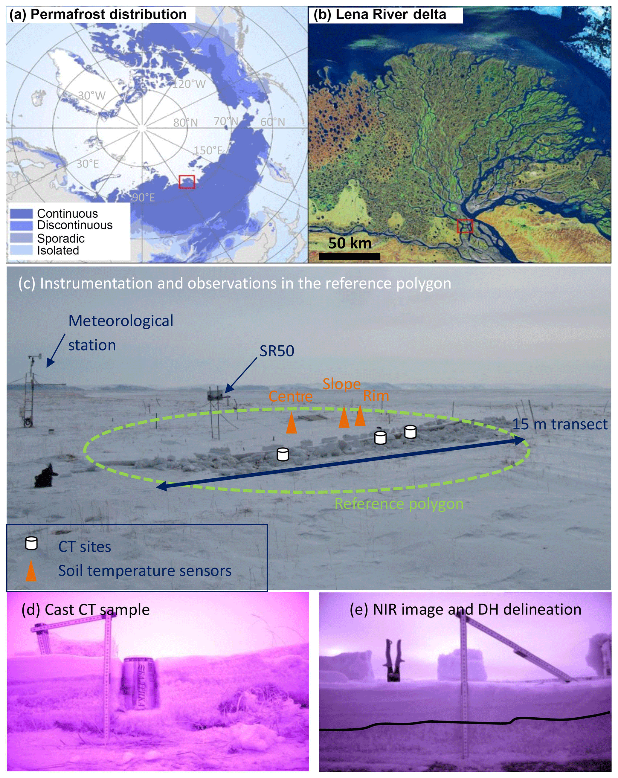
Figure 1Location of the Samoylov permafrost observatory within the continuous permafrost zone, Lena River delta (a, b); instrumentation and observations in the reference polygon (c); cast CT sample (d); NIR image of a transect's wall with the upper boundary of the DH layer delineated (e). See main text for abbreviations.
2.1 Samoylov site
The Samoylov permafrost observatory is located within the zone of continuous permafrost, on Samoylov Island in the Lena River delta, Siberia (72∘ N, 126∘ E; Fig. 1). The site has been used for intensive monitoring of ground temperatures and meteorological conditions since 1998 (Boike et al., 2008, 2013). The mean annual air temperature is −12.5 ∘C, with mean monthly temperatures ranging from −33 to 8.5 ∘C (1998–2011). The average annual rainfall is 125 mm, while snowfall averages 40 mm yr−1. The landscape is characterized by polygonal tundra, i.e. a complex mosaic of dry polygonal ridges with wet depressed centres, and a number of larger water bodies (Muster et al., 2012, 2013).
In the present study we analysed the snow properties with respect to the microtopography and surface conditions (water logged, grass covered, etc.) of the polygonal tundra. We divided the microtopography into polygon rims, slopes, and depressed centres, referred to simply as rims, slopes, and centres. With regard to the surface conditions, the elevated rims and slopes are usually vegetated (mosses and dryas species, ∼20 cm high) while the polygon centres are typically either damp or water logged. The damp centres are vegetated, mainly with mosses and Carex species (∼15 to 20 cm high) and are referred to as “grass centres” while the water-logged centres lie below the water table and are referred to as “ice centres”. The ponded water in these ice centres forms an ice base beneath the snow cover in winter and spring, which is clearly distinguishable from the moss–grass–snow interface of the grass centres. We therefore ended up with four microtopographic classes summarizing the typical microtopography and surface conditions at Samoylov: grass centres, ice centres, rims, and slopes.
During the winter the grasses of the rims, slopes, and grass centres tend to be flattened by snow and in places become intertwined at the base of the snowpack, up to a height of 7 to 10 cm (Fig. 1d).
2.2 Snow data
2.2.1 In situ snow observations
The Samoylov snow campaign in April 2013 (Fig. 1) focused on sampling the four aforementioned microtopographic classes in polygons located close to but not influenced by the Samoylov station. A total of 16 stratigraphic profiles were carried out, with records of grain type, size, occasionally density, hand hardness, and temperature measurements. Snow samples were cast with diethyl phthalate, as detailed in Heggli et al. (2009), and were later analysed in the SLF Davos cold laboratory using CT (Coléou et al., 2001; Schneebeli and Sokratov, 2004). Four sets of samples that covered the stratigraphy of distinct ice centre, grass centre, rim, and slope profiles were selected for our investigations on the basis of sample integrity. The corresponding sites will be referred to as CT sites (consisting of CT rim site, CT slope site, etc.). An east–west trench was excavated across a grass-centre polygon, which will be referred to as the “reference polygon” due to its denser instrumentation (Fig. 1). Near-infrared (NIR) images of the trench were realized to characterize the thickness of the basal DH layer along this transect at 50 cm spatial steps. The NIR images were treated in ImageJ (Schneider et al., 2012) with the following procedure: the green channel was extracted from the RGB image. The brightness and contrast was visually optimized based on the histogram. The average brightness of the full profile was 125, the DH region 106, and the surface layer 125 (brightness range 0–255). The boundary between these two main layers was measured based on a ruler put in the centre of the image. The resolution of the NIR images was better than 0.1 mm, so DH crystals and especially DH chains were in addition easy to discriminate from the upper layer with smaller, mostly rounded grains (RGs).
Snow depth was recorded continuously over the 2012–2013 snow season by an SR50 sensor (Campbell Scientific, ±1 cm accuracy, ±1 cm precision) located in the topographically low centre of the reference polygon (Fig. 1). This instrument acquires data over a circular surface of ∼20 cm in radius. However, this snow depth record differed from data acquired at grass-centre snow pits: on 21 April 2013 the SR50 measured 13 cm of snow while the transect, CT, and snow pit data indicated depths in excess of 17 cm for grass-centre conditions (Fig. 3). This difference is likely due to small-scale variability in snow depth induced by microrelief (notably vegetation tussocks) and in processes such as wind erosion immediately below the SR50 sensor: ancillary snow depth data acquired over a 14 m grass polygon transect at 20 cm spatial resolution show a 7 cm variance in snow depth and variations up to 9 cm over a 40 cm horizontal distance in centre conditions. To build a representative snow depth record for grass-centre conditions, we matched the SR50 snow data to the median of manually recorded snow depths at grass-centre snow pits (20 cm) on 21 April 2013 by multiplying the SR50 record by a constant factor of 1.6. The 7 cm offset in late April is consistent given the observed small-scale variability in snow depth. Finally, a time-lapse camera provided daily low-resolution images of the reference polygon.

Figure 2Meteorological, snow, and soil conditions at Samoylov over the 2012–2013 snow season.
2.2.2 Laboratory analysis
The samples cast in the field were transported to the cold laboratory in Davos and analysed with X-ray microtomography, thereby obtaining three-dimensional images of the structure and bonding of the ice crystals. Binary microtomographic images were used as input for a finite element analysis to calculate the three-dimensional heat conduction through the porous ice–air medium, based on the solution of the stationary (pore scale) heat equation, which is solved directly on the binary CT image. The effective conductivity tensor of the analysed sample is thereafter derived. This conductivity only takes into account pure conduction through the ice–air network, ignoring the effects of water vapour flux and latent heat. For the heat conductivity calculations we used the procedure described in Löwe et al. (2013), based on NIST finite element programs (Garboczi, 1998), with an air conductivity (ka) equal to 0.024 W m−1 K−1 and an ice conductivity (ki) equal to 2.43 W m−1 K−1. These values approximate the conductivity of the air and ice medium at temperatures between −15 and −20 ∘C (see https://www.engineeringtoolbox.com/, last access: 1 January 2018, and data compiled by Waite et al., 2006), causing a maximum error in retrieved Keff of less than 4 % for a snowpack between 0 and −40 ∘C (estimation based on the parametrization from Löwe et al., 2013, using the values of ka and ki).
2.3 Soil temperature data
Soil temperatures were recorded over the 2012–2013 snow season from three profiles within the reference polygon (rim, slope, and grass centre) at depths of 5, 20, and 40 cm, using thermistors (temperature probe model 107, Campbell Scientific Ltd., UK). The thermistors were calibrated at 0 ∘C so that the absolute error was less than 0.1 K over a temperature range of ±30 ∘C.
2.4 Meteorological data
The SNOWPACK and CryoGrid3 models require as input the following meteorological data: 2 m air temperature, incoming shortwave and longwave radiation, wind speed, and relative humidity of the air. We drive the models with snow depth recorded by the SR50 sensor instead of precipitation. Air temperature and relative humidity were recorded at the Samoylov meteorological station using an HMP45C air temperature and humidity sensor (Fig. 1). Unfortunately the sensor became saturated at temperatures below −40 ∘C and so for the period between 1 February and 15 March 2013, when the air temperatures regularly dropped below −40 ∘C, we used air temperature records from the ERA-Interim reanalysis (ERA-I; Dee et al., 2011) instead. The ERA-I data were linearly interpolated from their native 3-hourly temporal resolution (analysis and forecast fields) to a 30 min time series to drive SNOWPACK. This substitution seems appropriate since for the rest of the 2012–2013 winter period, ERA-I temperatures show a high correlation with Samoylov observations (r2=0.97) and a low bias (−0.9 ∘C). ERA-I fields were also proven to be a high-quality source of driving variables to simulate the evolution of the northern Eurasian snowpack including Siberia (Brun et al., 2013), with minor differences between station data and grid field over large, rather flat areas like the Lena River delta. Finally, a comparison of ERA-I with locally acquired meteorological data from earlier years at Samoylov confirmed this validity for the skin surface temperature, which responds very sensitively to differences in the driving variables (Langer et al., 2013).
Incoming shortwave and longwave radiation were measured at the Samoylov meteorological station with an NR01 Hukseflux four-component net radiation sensor. Wind speed was measured at 2.5 m above ground with a 05103 Young wind monitor. Wind speed was (together with air temperature) the only meteorological field for which likely instrumental failure was detected, characterized by periods of a few hours to a few days with null wind speed. The impact on the SNOWPACK simulations is however marginal as no major snow depth variation was observed during these periods.
Snow depth data, meteorological data, and data on the ground thermal conditions at Samoylov during the 2012–2013 snow season are presented in Fig. 2. Meteorological and snow depth data are freely available (Boike, 2017).
2.5 SNOWPACK snow model
SNOWPACK is a one-dimensional, physically based snow-cover model. Driven by standard meteorological observations (see Sect. 2.4), the model simulates the stratigraphy, microstructure, metamorphism, temperature distribution, and settlement of snow, as well as surface energy exchange and mass balance. Snow is represented by a number of state variables (temperature, density, and water content) and the snow microstructure by grain characteristics (grain size, size of bonds, sphericity, and dendricity), which allow a diagnostic of the grain type (Lehning et al., 2002b). The equations governing the evolution of the seasonal snowpack are described in Bartelt and Lehning (2002) and Lehning et al. (2002a, b), along with the parameterizations adopted for important snow properties, such as Keff−z. The latter is based on the work of Adams and Sato (1993), who considered the geometrical arrangement of spherical ice grains to derive an analytical formulation for Keff−z. The thermal effect of water vapour diffusion within grain interstices and the temperature dependence of ice conductivity are also taken into account in the parameterization currently used in SNOWPACK. A shape factor calibrated with alpine snow is used to take into consideration the non-sphericity of the snow grains. The SNOWPACK formulation for Keff−z depends in the end on three variables: temperature, density, and the ratio between grain-size and bond size.
The SNOWPACK model was originally developed for alpine conditions (Lehning and Fierz, 2008) but has been recently adapted to different snow and meteorological conditions for the instance of the extreme conditions of the Antarctic Plateau at Dome C: the latter required a specific treatment of the effects of high wind speeds and low temperatures on snow accumulation, compaction, and settlement (Groot Zwaaftink et al., 2013).
2.6 CryoGrid3 permafrost model
CryoGrid3 (CG3; Westermann et al., 2016) is a one-dimensional permafrost–soil model that has been extensively adapted and validated for the Samoylov conditions (Westermann et al., 2016; Langer et al., 2016). Since the soil scheme in SNOWPACK lacks the detail and performance of CG3, we used CG3 to model the ground thermal regime but using the snow characteristics (density, depth, and bulk thermal conductivity) produced by SNOWPACK as input.
CG3 is forced by standard meteorological variables (see Sect. 2.4) which drive an explicit surface energy balance scheme that simulates the exchange of heat and water with the atmosphere. The model includes a transient heat transfer scheme for the soil that is specifically optimized for simulating freeze–thaw processes within permafrost. The soil physical properties such as heat capacity, thermal conductivity, and freeze curve are derived according to a parameterization suggested by Dall'Amico et al. (2011). The soil composition is assumed to be constant, so that any changes in soil moisture other than those due to phase changes are ignored. This assumption is well justified as the soils at Samoylov are almost completely saturated (Langer et al., 2013). CG3 also includes a simplified snow cover representation that only takes into account a limited number of the natural processes that occur in snowpacks. It is therefore not comparable to more sophisticated snow models such as SNOWPACK or CROCUS. Therefore, in our simulations with CG3, the snow properties involved in conductive heat transfer were taken either from SNOWPACK simulations (in Sect. 5) or derived from an external construction (in Sect. 6), bypassing the CG3 estimates for these properties. All other properties or processes were calculated by CG3: this includes an exponential damping of incoming shortwave radiation with snow depth, assuming a constant light extinction coefficient (e.g. O'Neill and Gray, 1972) and a snow albedo decreasing with snow ageing (Westermann et al., 2016).
3.1 Composition and properties of individual layers
As in other tundra snowpacks described in literature, the Samoylov snowpack was largely made up of basal DH and of wind slabs with small RGs (Figs. 3 and 4). Based on the four profiles investigated by CT, the DH layers and wind slabs exhibited significantly distinct densities and Keff−z (Fig. 3, p values <0.05 for a two-sided t test): the DH layers had a mean density of 236 kg m−3 and a mean Keff−z of 0.22 W m−1 K−1, while wind slabs had a mean density of 356 kg m−3 and a mean Keff−z of 0.36 W m−1 K−1. The general characteristics of the snowpack at the CT sites (grain types, snow depth, DH thickness-to-total snow depth ratio) were very similar to the median characteristics retrieved at the other snow pits dug in each microtopographic class (Fig. 4), which made them representative for their microtopographic class. The only exception is the CT slope profile, which features an exceptionally high proportion of DH (80 %, while the median for slope sites was 50 %).
In the middle or upper part of the snowpack at vegetated sites, we found DH layers exhibiting a higher density (up to 300 kg m−3), together with a higher conductivity (above 0.3 W m−1 K−1), higher hand hardness (2 to 3), and smaller grain sizes (1 to 2 mm) than basal DH (hand hardness 1, grain size 5 to 10 mm). These dense DH layers have probably been formed by the metamorphism of former wind crusts (i.e. they are indurated DH), thereby retaining a high density. They were all found above the vegetation layer, where wind effects are likely to be more pronounced.
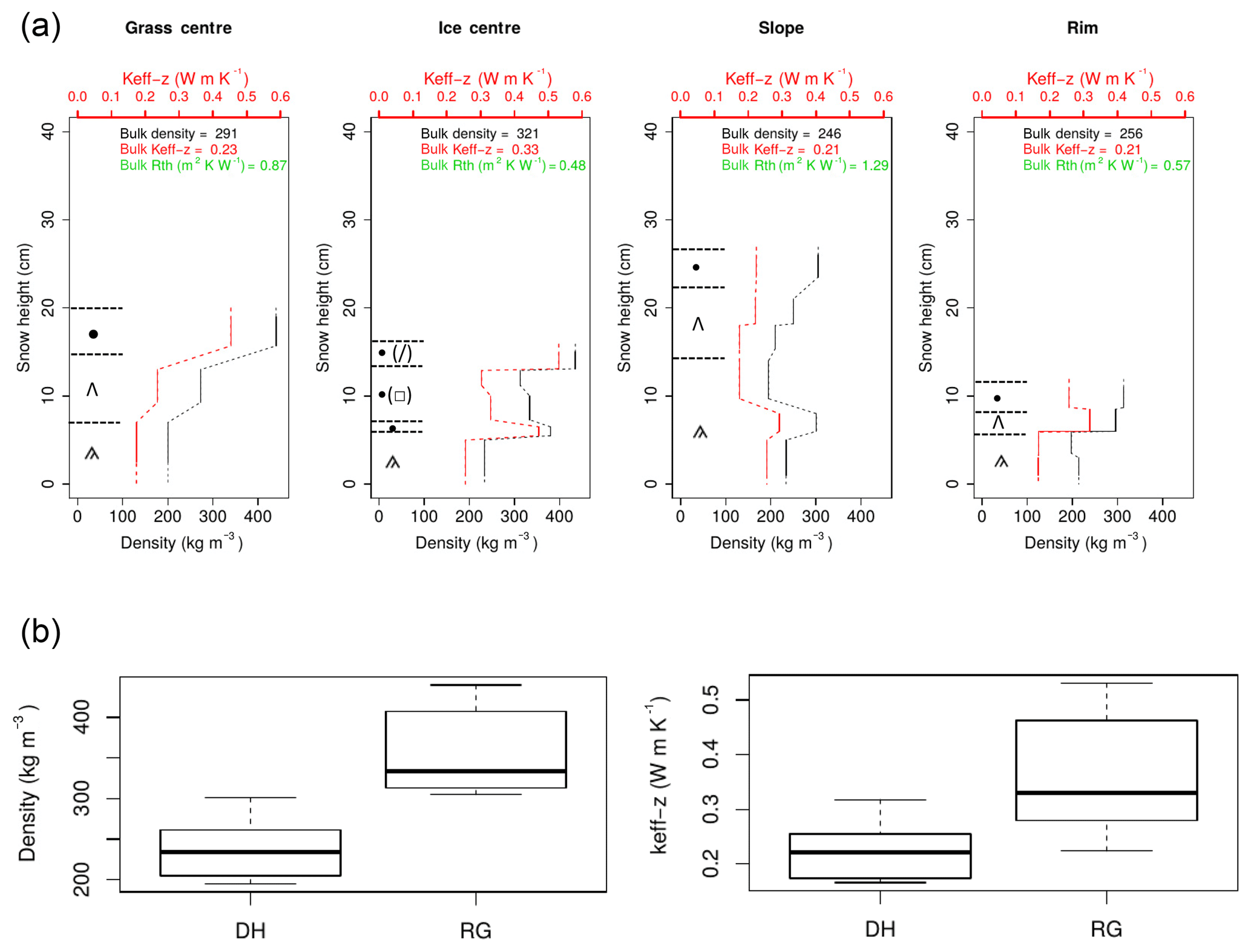
Figure 3(a) Grain shape, density, and Keff−z profiles from the four CT sites. Density and Keff−z values are represented by piecewise constant functions over the layers where the CT analysis was performed; these segments are connected by a dashed line as a guide to the eye. Symbols for the grain shapes originate from Fierz et al. (2009). When several grain shapes coexist within a layer, the dominant type is listed first. (b) Box plots of density and Keff−z for individual DH layers (11) and rounded grain (RG) layers (eight) found within the CT profiles. RG shapes were occasionally associated with faceted crystals and decomposing and fragmented precipitation particles.
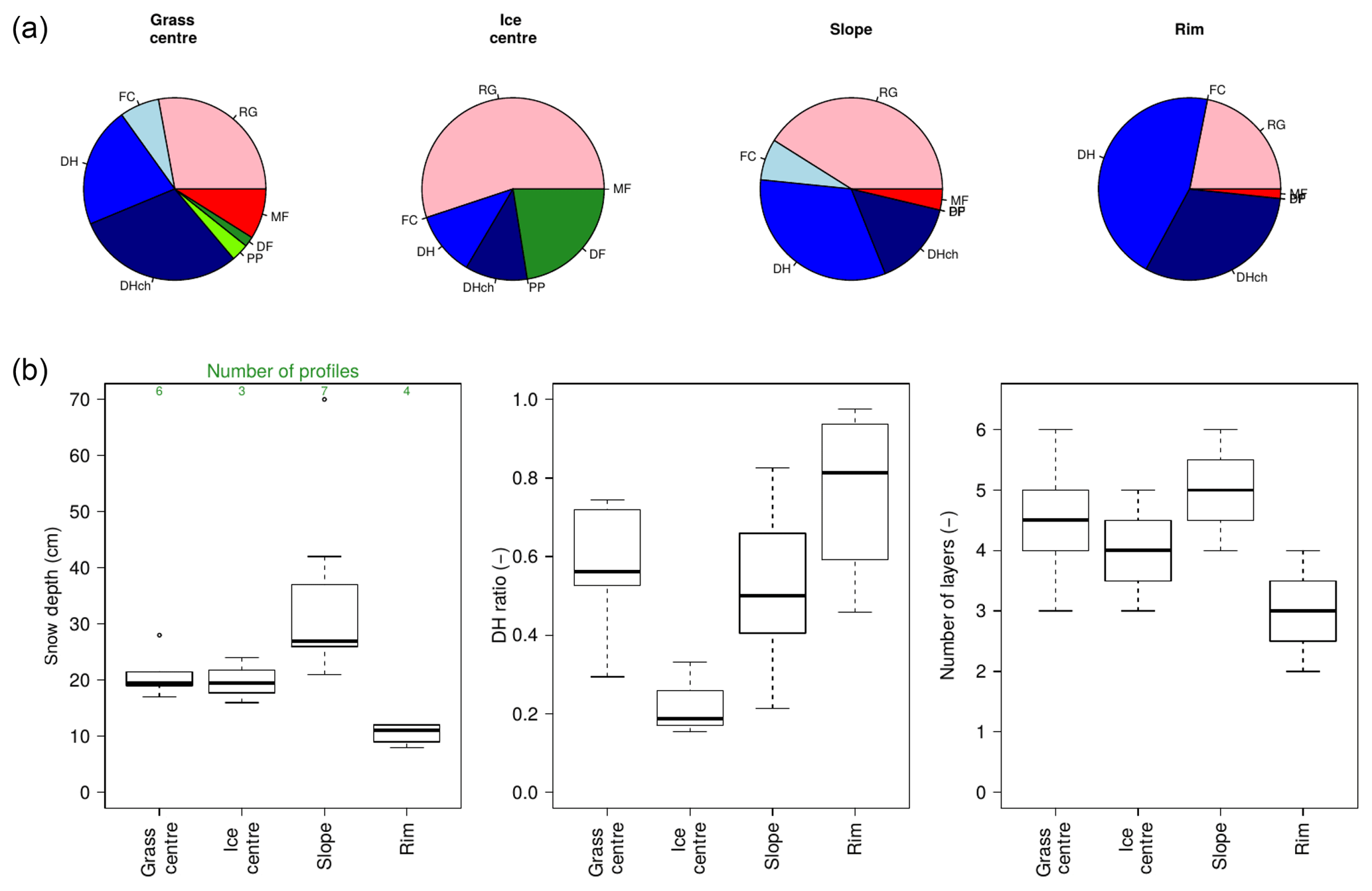
Figure 4Mean composition (a) and median characteristics (b) of the Samoylov snowpack in the four microtopographic classes. These statistics include the observations from the 16 snow pits and the four CT sites. DH ratio is the DH thickness-to-total snow depth ratio, also called α in the paper. The abbreviations for the main grain types come from Fierz et al. (2009): PP: precipitation particles; DF: decomposing and fragmented precipitation particles; RG: rounded grains; FC: faceted crystals; DH: depth hoar; DHch: chains of DH; MF: melt forms.
3.2 Spatial variability
Microtopography and surface conditions clearly play a role in shaping the snowpack conditions at Samoylov. Based on our 16 snow pits and four CT profiles, we found the snow to be significantly deeper at slope sites and shallower at rim sites (27 cm vs. 10 cm median depths, p value <0.1 for a two-sided t test) than at the centre sites (19.5 cm median depth). This observation has often been reported in literature from other tundra sites (e.g. Wainwright et al., 2017): indeed, the rim sites are the most exposed to wind and receive reduced deposition during blowing snow events, while slopes, especially those on the lee side, experience lower wind speeds and enhanced deposition. The larger number of distinct snow layers found in slope profiles is further evidence of that process. In contrast to snow depth, the DH thickness-to-total snow depth ratio (hereafter α) was lower on slopes and higher on rims (0.5 vs. 0.8, median values; difference not significant at the 95 % level). Rim profiles also exhibited a larger proportion of DH chains (i.e. vertically structured DH crystals in which most of the lateral bonds have disappeared; Fierz et al., 2009) than the other microtopographic classes: this is in line with an increased temperature gradient as a result of shallower snow depths. Grass-centre and ice-centre sites had very similar snow depths but a significantly lower proportion of DH was found at ice centres than in the other classes. This is easily explained by the higher conductivity of ice when compared to frozen ground (even saturated), which promotes colder temperature in the uppermost centimetres of frozen ponding water than in a frozen ground surface, and hence reduced temperature gradients through the snow when snow onset occurs after initial freezing. Basal DH crystals formed over ice are therefore smaller (4 to 6 mm) than those found at grass-centre sites (6 to 8 mm).
We calculated the bulk Keff−z(Kbulk) at each CT site by weighted harmonic mean of the Keff−z of individual snow layers. Kbulk showed little variation among the three CT sites with underlying grasses: Kbulk was 0.21 W m−1 K−1 at the CT rim and slope sites and 0.23 W m−1 K−1 at the CT grass-centre site (Fig. 3). A more representative slope site with a lower proportion of DH portion would probably have had a slightly higher Kbulk value. A much higher Kbulk, 0.33 W m−1 K−1, was however obtained at the ice-centre site, where much less DH had developed.
We tested the assumption that differences in the DH thickness-to-total snow depth ratio (α) can mostly explain the variability in Kbulk across the four CT sites. For this we relied on the approach by Zhang et al. (1996), who considered that an Arctic snowpack can be approximated by two homogeneous layers, a DH layer and a wind slab, each with its own distinctive density and Keff−z value. Rutter et al. (2014) also used a similar approach for microwave emission modelling. Following this approach, Kbulk is expressed by
where KDH and Kcrust are the Keff−z for DH and wind crust layers, which we here approach by their mean values in our CT samples (0.22 and 0.36 W m−1 K−1, respectively). Kbulk is thus a decreasing function of α. We found that 72 % of the variability in Kbulk among our four sites can be explained by this simple two-layer approach.
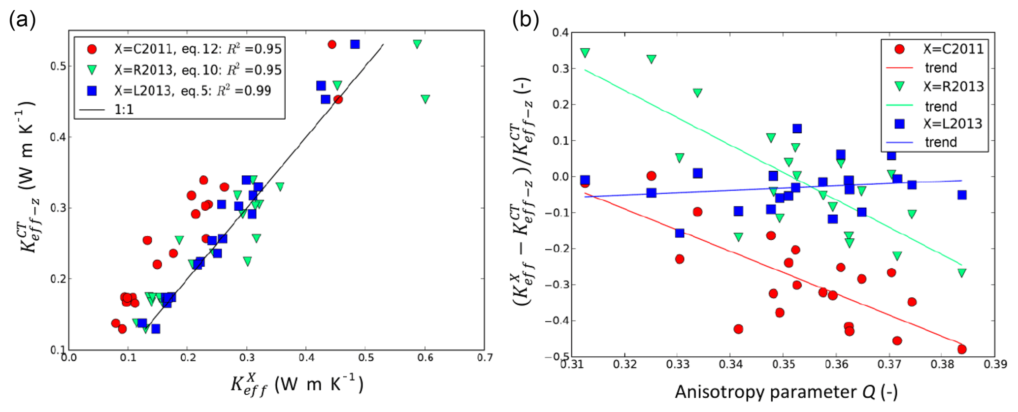
Figure 5(a) Comparison between estimates of Keff or Keff−z made with the CT method () and estimates made using parameterization “X” (, where X= C2011, R2013 or L2013: see paper for description of these parameterizations). (b) Relative bias in with respect to as a function of the anisotropy parameter Q. Each point represents a snow sample analysed by CT in this study.
The insulating power of a snowpack is characterized by the thermal resistance (see Sect. 1). Hence, the variations in snow depth HS across our four sites, as shaped by microtopography (see Sect. 3.1), also affect the local insulating power of the snowpack. Indeed, we found that the ice-centre profile has a very low Rth (0.48 m2 K W−1) due to a high Kbulk and a moderate snow depth. The Rth of the snowpack however increases from the rim site (0.57 m2 K W−1), through the grass-centre site (0.87 m2 K W−1), to the slope site (1.59 m2 K W−1): this increase follows the increase in snow depth among these sites (from 10 to 19.5 and 27 cm, respectively), despite variations in the Kbulk values (which at times also increase with snow depth).
Our observations suggest that, when there is basal vegetation present, Rth is more sensitive to variations in total snow depth than to variations in the DH proportion α, which controls Kbulk. We assessed this by looking at the sensitivity of Rth to α and HS in the two-layer approach. Rth is expressed by
implying a sensitivity to variations in and a sensitivity to variations in expressed by:
We estimated bounds of 3.5–4.3 and 0.17–0.71 m2 K W−1 for these sensitivities, respectively, considering the following ranges for α and HS: α=0.4–0.9 and HS=0.1–0.4 m. The HS decreased by 0.1 m from the CT grass-centre profile to the CT rim profile, while α increased by 0.22. From the median grass centre profile to the median slope profile, HS increased by 0.08 m while α decreased by 0.06. With these orders of magnitudes, it appears clearly that variations in HS have a greater influence than variations in α on the insulating power of snow across the polygonal microtopography when there is basal vegetation present.
3.3 Assessment of existing Keff−z parameterizations
In the four CT profiles Keff−z showed a strong correlation with density (r=0.94). We investigated the ability of three different parameterizations for Keff or Keff−z to match the values obtained with our measurements (Fig. 5). These parameterizations are from Calonne et al. (2011), Riche and Schneebeli (2013), and Löwe et al. (2013), and we refer to them hereafter as C2011, R2013, and L2013, respectively. C2011 expresses the mean of the vertical and horizontal components of Keff as a density-based regression. R2013 expresses the vertical component of Keff (Keff−z) as a density-based regression inferred from DH and faceted crystals (FCs) samples only, that is to say, grain types with a marked vertical anisotropy. Finally, L2013 is a regression of Keff−z based on density and anisotropy. It relies on an anisotropy parameter, Q, calculated directly from CT images based on the two-point correlation function (Löwe et al., 2013, their Eq. 4). Q is above 0.33 (below 0.33) when the snow grain arrangement shows preferential vertical (horizontal) connections.
With respect to our data, there is an improvement in performance from C2011 (good correlation but noticeable bias) to R2013 (good correlation, reduced bias), and finally to L2013 (improved correlation and reduced bias). C2011 does not take anisotropy into account, nor does it attempt to represent the vertical component of the conductivity (Keff−z), which probably explains its relatively poor performance. A bias in R2013 for snow types with horizontal anisotropy (Q<0.33) is to be expected as R2013 is designed to represent the Keff−z of vertically anisotropic grains. Our results confirm that R2013 is indeed biased on samples with Q<0.33 (Fig. 5b), consisting of RG and partly decomposed–fragmented particles (DFs). R2013 also underestimates Keff−z in the samples with the greatest vertical anisotropy, which may be due to the very small number of samples (only two) used by the authors to constrain their parameterization at densities greater than 300 kg m−3. Being derived from a density-based regression, R2013 is furthermore structurally incapable of taking into account all possible degrees of anisotropy encountered in nature. The best performance was obtained with L2013, which confirms the importance of anisotropy in Keff−z estimations. The two largest biases obtained from regressions based on density only (underestimations of Keff−z by 47 % and 49 %) were obtained using C2011 on DH chains, i.e. on highly anisotropic grain forms.
In Sect. 1 we recalled that adaptations were required for the current generation of snow models if realistic density profiles (and consequently Keff−z profiles) were to be simulated in Arctic conditions. These adaptations concerned wind densification (WIND), the water vapour transport occurring under steep temperature gradients (VAP), and the mechanical, optical, and metamorphic effects of basal vegetation protruding into the snowpack (VEG). The traditional density-based formulations for Keff−z also needed to improve and incorporate the effect of grain anisotropy (ANISO).
Some of the effects of VEG (mechanically reduced compaction, enhanced grain growth) and VAP (reduced density in the basal layers as a result of upward flux, enhanced grain growth) are hard to disentangle in Arctic conditions, where they contribute to both density reduction and enhanced grain growth in basal layers. Furthermore, no explicit description of water vapour transport and associated metamorphism is available in the current snow models. We therefore chose to address both VAP and VEG together: both effects are comprised in the phenomenological “VEG” adaptation, described below.
For the mechanical effect of VEG we reduced the fresh snow density (ρ0) for snow that occurs within the grasses, i.e. up to a thickness of 7 cm. The underlying hypotheses are that (i) while snow has not filled the snow-holding capacity of the basal vegetation, snow is not available for transport (Liston and Elder, 2006) and therefore snow accumulation in the grass-layer consists in precipitation particles of lower density than typical wind-blown RGs, and (ii) that grasses form a rigid structure that protects snow from wind compaction and introduces macroscopic voids that reduce its density. Different ρ0 values were tested and 150 kg m−3 was chosen as giving the best match to end-of-season in situ density observations. Domine et al. (2016a) chose to increase the dry snow viscosity in the CROCUS snow model by a factor of between 10 and 100 in order to take into account the limited snow compaction within the stems of shrubby vegetation. In our case, however, an alternative approach was required since self-compaction is very limited in the thin Samoylov snowpack. Note that our approach however differs from the SnowModel (Liston and Elder, 2006) in the sense that we focus on snow structure and properties (density, Kth) as influenced by the wind conditions, while the SnowModel and its blowing snow sublimation and redistribution scheme SnowTran3D target the spatial distribution and time evolution snow water equivalent and the way they are affected by vegetation.
The optical effect of VEG (i.e. the absorption of solar radiation by grasses and sandy impurities, which are common at Samoylov) was not taken into consideration but is addressed later in Sect. 7.
The metamorphic effect of VEG was addressed by enhancing bond and grain growth rates by a constant factor within the grass and snow layer. This phenomenologically represents the favourable conditions for grain growth within airy vegetation layers. We feel justified in taking this approach because the current metamorphism and diffusion laws of the snow models are unable to reproduce the commonly observed grain sizes in excess of 10 mm in basal DH layers accommodating vegetation. A factor of 5 was selected as best reproducing the observed end-of-season DH grain sizes at Samoylov. Both bond and grain growth rates were enhanced by the same factor in order to keep their ratio constant, as this ratio governs a number of mechanical and thermal properties in SNOWPACK.
For WIND, we built on the work by Groot Zwaaftink et al. (2013), who designed an adaptation of SNOWPACK to Antarctica Dome C conditions. These authors considered that effective snow deposition on the surface occurs only during wind events, i.e. periods when the wind speed averaged over 100 h (U100−h) exceeds a 4 m s−1 threshold (U0=4 m s−1). The density of fresh snow (ρnewsnow) is then a logarithmic function of U100−h:
The use of this approach is justified at Samoylov as wind conditions at the Samoylov station (mean annual wind speed 3.6 m s−1) are comparable to those at Dome C (mean annual wind speed 2.9 m s−1), and more than 50 % of snow deposition at Samoylov occurs during wind events. Groot Zwaaftink et al. (2013) used ρ0=250 kg m−3 as the lowest fresh-snow density. However, no value as low as that was recorded during the 2013 program from the wind slab layers at Samoylov, where the density is always above 305 kg m−3. Such densities are furthermore essentially achieved by wind compaction (settlement in thin arctic snowpacks is negligible). We therefore used ρ0=305 kg m−3 in Eq. (5). The original value for Δρ(Δρ=361 kg m−3) was retained.
For the ANISO adaptation we implemented in SNOWPACK an alternative formulation derived from L2013 (Löwe et al., 2013, their Eq. 5), which by considering anisotropy, explained a larger part of the observed variability in our Keff−z measurements than formulations relying solely on density. However, L2013 requires an anisotropy parameter Q, which can be either calculated from CT images of samples or estimated from polarimetric radar data (Leinss et al., 2016), but is not yet included in current snow models. In order to implement L2013 in SNOWPACK, we therefore had to derive an empirical relationship between Q and a modelled microstructural parameter. To this end, we used the data from Löwe et al. (2013) to obtain statistical regressions between Q and the optical equivalent diameter of snow grains. We calculated these regressions for different grain type classes: RGs, DH, FCs, DFs, and melt forms, most of which indicate reasonable linear dependences. These regressions were used in SNOWPACK in order to derive the parameter Q, using normalized grain size (within each grain type class) as a proxy for normalized optical diameter. We only took into account anisotropy for the RG, DH, and FC grain types, as these are the dominant grain types in the Samoylov snowpack. Regression coefficients and implementation details are in Appendix A.
The three adaptations (WIND, VEG, and ANISO) can also be combined. Simulations were initially carried out for the default SNOWPACK set-up (DEFAULT) and for each of these adaptations individually, but both the WIND and VEG adaptations proved to be essential for the Samoylov snowpack conditions to be reasonably well reproduced. Results are therefore shown in this paper for the followingset-ups, each combining one or more adaptations. All set-ups except the one including the ANISO adaptation rely on the original Keff−z parameterization from SNOWPACK described in Sect. 2.5.
-
DEFAULT
-
WIND
-
WIND + VEG
-
WIND + VEG + ANISO
We carried out simulations with SNOWPACK and CG3 to represent the snow and ground conditions in the grass centre of the reference polygon, where the SNOWPACK snow forcing data were acquired (see Sect. 2.2.1) and CG3 soil properties calibrated (see Sect. 2).
5.1 Snow simulations
The adaptations to SNOWPACK enable a reasonable simulation of the Samoylov snowpack (Figs. 6 and 7), but both VEG and WIND adaptations are critical. While all set-ups consistently produce a thick basal DH layer at the end of the season, DEFAULT simulates a density profile that has too low of a mean value (190 kg m−3) when compared to the CT grass centre (290 kg m−3) and to the average value for the four CT profiles (279±34 kg m−3). This simulated density profile is also inverted, featuring higher values at the bottom and illustrating the typical bias highlighted by Domine et al. (2016b) and Barrere et al. (2017). Bulk Keff−z obtained using DEFAULT is likewise too low compared to observations (0.11 vs. 0.23 W m−1 K−1 for the CT grass centre) and is also inverted. This low bias is likely to have caused the rapid growth of DH in this set-up, as a low Keff−z favours steep temperature gradients. The low density and Keff−z biases can be corrected by using the WIND option, which in its current form tends to overestimate bulk density. However, the WIND option alone produces quite flat (i.e. vertically uniform) density and Keff−z profiles. The VEG adaptation is then needed to produce a correct shape for these profiles, with higher values at the top and lower values at the base. Thus, while the WIND option on its own reduces the DH growth due to dense and conductive bottom snow, the addition of the VEG option introduces lower densities and Keff−z values for the basal layers and permits a more rapid and thicker growth of DH.
Combining the WIND and VEG options therefore yields reasonable simulations of bulk Keff−z (0.20 W m−1 K−1) and density (305 kg m−3). When the ANISO option is introduced (WIND + VEG + ANISO), the simulated bulk Keff−z (0.24 W m−1 K−1) also agrees well with the CT grass-centre estimate (0.23 W m−1 K−1), while the interlayer variability in Keff−z is enhanced, thus better reflecting the observed interlayer variability (Fig. 7). It is interesting to note that both the WIND + VEG and the WIND + VEG + ANISO set-ups produce a DH layer that is up to 10 cm thick at the end of the snow season, above the vegetation layer: this means that former wind crusts have been transformed into DH, producing the indurated DH layers reported in observations.
Finally, all SNOWPACK set-ups produce a thick layer of FCs in the upper part of the snowpack, but FCs were rare in the late April 2013 Samoylov snowpack (Fig. 4). We interpret this as a likely bias in SNOWPACK that results in too rapid formation of FCs. Conversely, it is possible that a wind event on 10 April 2013 contributed to the high number of RGs found in the 21 April manual and CT profiles. Because it brought a very low accumulation at the SR50, this event was not captured in simulations with the WIND option.

Figure 6SNOWPACK grain shapes in the four simulation set-ups. The colour code was complemented with grain shape symbols after Fierz et al. (2009) for the 20 May 2013 profile (representative of the time of the snow campaign).
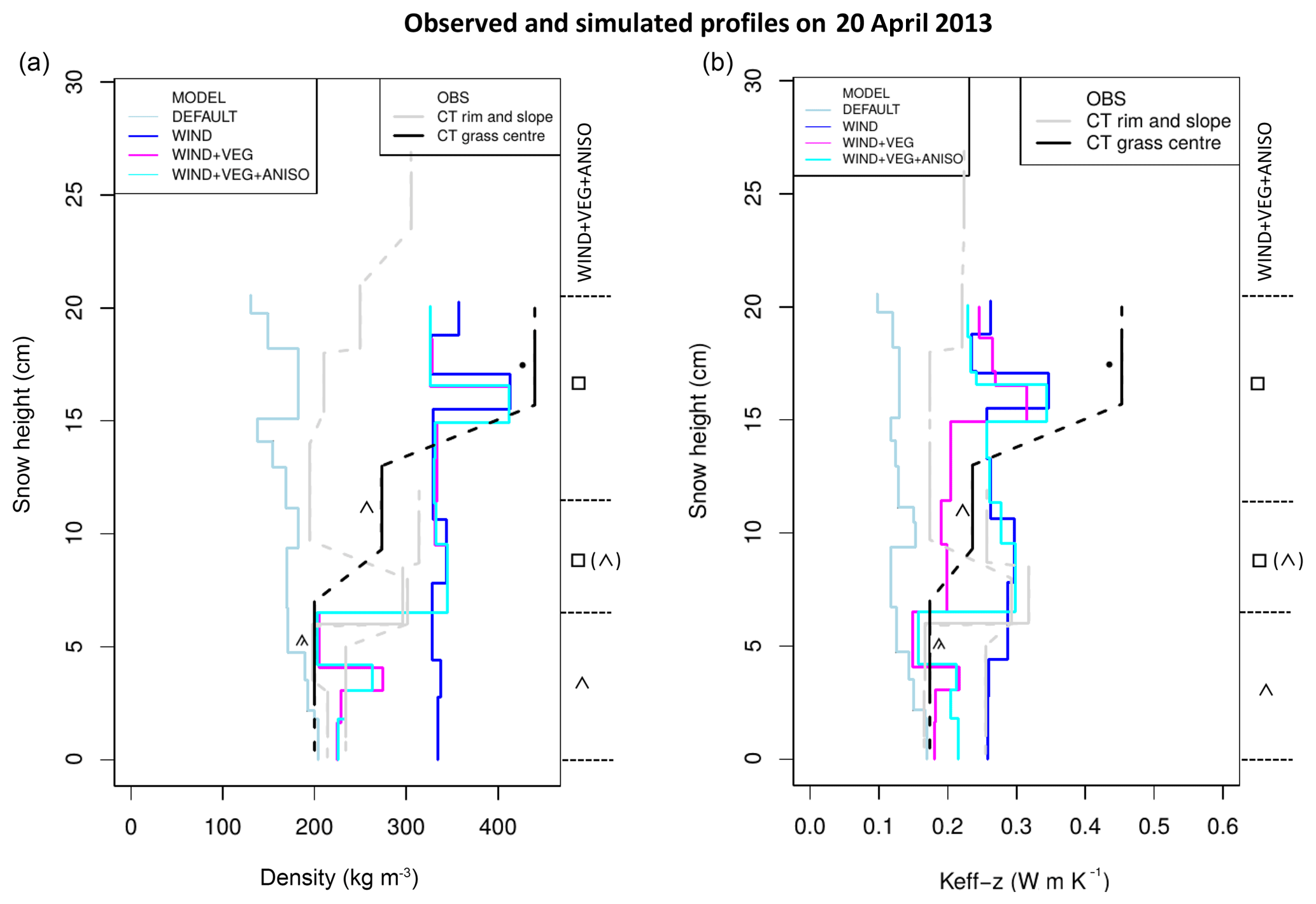
Figure 7Observed and simulated density and Keff−z profiles on 20 April 2013. Observations (OBS) are the estimates made using the CT method at the three CT sites with basal vegetation; grain shape is indicated on the plot for the CT grass-centre site. Simulations (MODEL) were made with the four SNOWPACK set-ups; grain shape is indicated at the side for the WIND + VEG + ANISO set-up.
5.2 Soil simulations
The ground thermal regime at the grass centre of the reference polygon was simulated by CG3 over the 2012–2013 snow season using snow properties calculated in SNOWPACK with the DEFAULT, WIND, WIND + VEG, and WIND + VEG + ANISO set-ups. These simulations were compared with the soil temperature measurements from the same grass-centre site. The reference polygon also hosts soil temperature measurements from a rim and a slope site: the spatial variability reflected in these three measurements was also considered and is referred to as “observed variability” in soil temperatures in both the text and figures.
To analyse the modelling performances we split the winter into four phases:
-
Phase 1 is freezing from 1 October (snow onset) to 7 November.
-
Phase 2 is cooling from 7 November to 20 February (dark winter followed by a period with low-angle solar radiation).
-
Phase 3 is warming from 20 February to 5 May (melt-out date).
-
Phase 4 is thawing from 5 to 31 May.
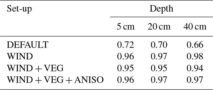
The WIND, WIND + VEG, and WIND + VEG + ANISO set-ups produced soil temperatures in good agreement with the grass-centre measurements (Fig. 8, Table 1), especially during freezing and cooling phases: the deviation from the measured soil temperatures when using the WIND + VEG + ANISO set-up was of the same order of magnitude as the observed variability, while the deviations when using the WIND and WIND + VEG set-ups were slightly greater. The DEFAULT set-up yielded a clear overestimation of soil temperatures at all depths, which could not be explained by the observed spatial variability in soil temperatures. This bias started during the freezing phase and persisted throughout the snow season; it is likely to be caused by the underestimation of Keff−z in the DEFAULT set-up (see Sect. 5.1), which also starts in the early snow season during rapid DH formation. In light of the good agreement between our Keff−z estimates by CT and the simulated Keff−z profiles in the WIND + VEG + ANISO set-up (Sect. 5.1), we interpreted these results as confirming the soundness of our CT estimates for Keff−z.
The performance of the WIND, WIND + VEG, and WIND + VEG + ANISO set-ups deteriorated during the warming phase, when all simulations at first showed a systematic warm bias, which then turned into a cold bias at the start of the thawing phase. The warm bias during the warming phase suggested that limitations exist in the modelling of energy transfer processes within the snow, as here modelled by CG3. We formulated two hypotheses.
-
Deficiencies in the parameterization of radiative heating within the snowpack may be involved as the bias concurs with the increase in shortwave radiation.
-
The formation of an air layer at the base of the natural snowpack (as a result of mass depletion due to a sustained upward vapour flux throughout the winter) may increase its insulating power as the season advances. The formation of such an air layer within an Arctic context has previously been reported by Domine et al. (2016b) but is not represented in the adapted SNOWPACK and therefore in the thermal properties passed to CG3.
Table 1Nash–Sutcliffe model efficiency criteria (Nash and Sutcliffe, 1970) between the soil temperature simulations and measurements at different depths in the grass centre of the reference polygon.
We tested the thermal impact of both hypotheses by conducting sensitivity simulations in which the following was carried out.
-
The penetration of radiation into the snowpack was switched off in the CG3 model. This was performed for the four SNOWPACK set-ups.
-
We inserted an air layer (with W m−1 K−1) at the base of the snowpack during the warming phase, growing in a linear fashion from 0 to 1.5 cm during the warming phase. This was done by modifying the snow properties from the WIND + VEG + ANISO set-up and resulted in a linear reduction in bulk Keff−z from 0.23 to 0.16 W m−1 K−1 over that period.
Suppressing the penetration of solar radiation in the snowpack considerably reduced the warm biases in soil temperatures during the warming phase for all WIND set-ups, while leaving their performances during the freezing and cooling phases unaffected (Fig. 9). While physical reasons for a likely bias in radiative transfer in CG3 will be advanced in Sect. 7, the remaining simulations in this study were carried out with the solar radiation penetration switched off. The air layer hypothesis did not, however, lead to any visually identifiable change in the simulations. This reveals a very low sensitivity of the soil thermal regime to variations in snow thermal conductivity during the warming phase.
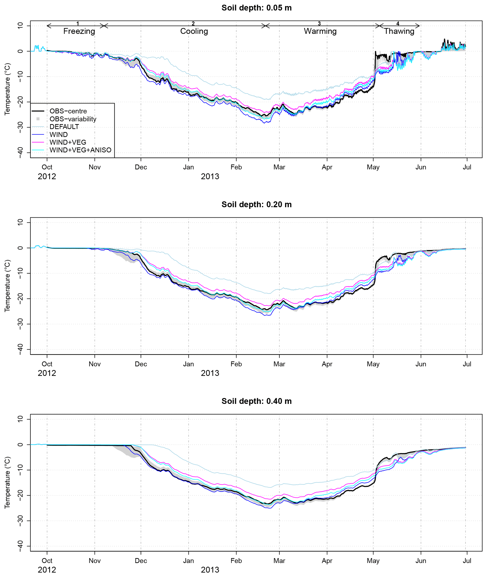
Figure 8Simulated vs. observed soil temperatures at depths of 5, 20, and 50 cm in the reference polygon's grass centre. OBS variability (grey shading) is the envelope of observed soil temperatures from the monitored rim, centre, and slope soil sites. The winter phases from Sect. 5.2 have been reported.
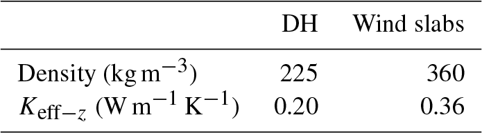
We made use of data from the reference polygon transect to more thoroughly characterize the spatial variability in snow depth, structure, and insulating power across the polygonal tundra at Samoylov. We extracted DH thickness and snow depth at 31 points with 50 cm spacing along the transect by post-processing the NIR images (Fig. 1e, Sect. 2.2.1). The two-layer approach by Zhang et al. (1996) (see Sect. 3) was then used to infer bulk Keff−z, Rth, and density at these 31 points at the time of the field observation (21 April 2013), relying on Eqs. (1) and (2). Time series of these bulk snow properties were then computed, based on the two-layer approach and time evolution of the DH properties as simulated by the WIND + VEG + ANISO set-up providing the best match to observed snow characteristics. Wind slab properties were considered constant in time and equal to their end-of-season values (mean of CT estimates for wind slabs from April 2013 samples; Table 2). The hypotheses behind the construction of these time series and other relevant details are given in Appendix B.
This approach led to a small spread in Kbulk during the whole snow season (from 0.22 to 0.29 W m−1 K−1) and a much higher dispersion in Rth (from 0.45 to 1.2 m2 K W−1), which reaches a maximum towards the end of the season where it covers a range similar to that inferred from CT analysis at the three CT sites with basal vegetation (from 0.48 to 1.59 m2 K W−1; Fig. B2)
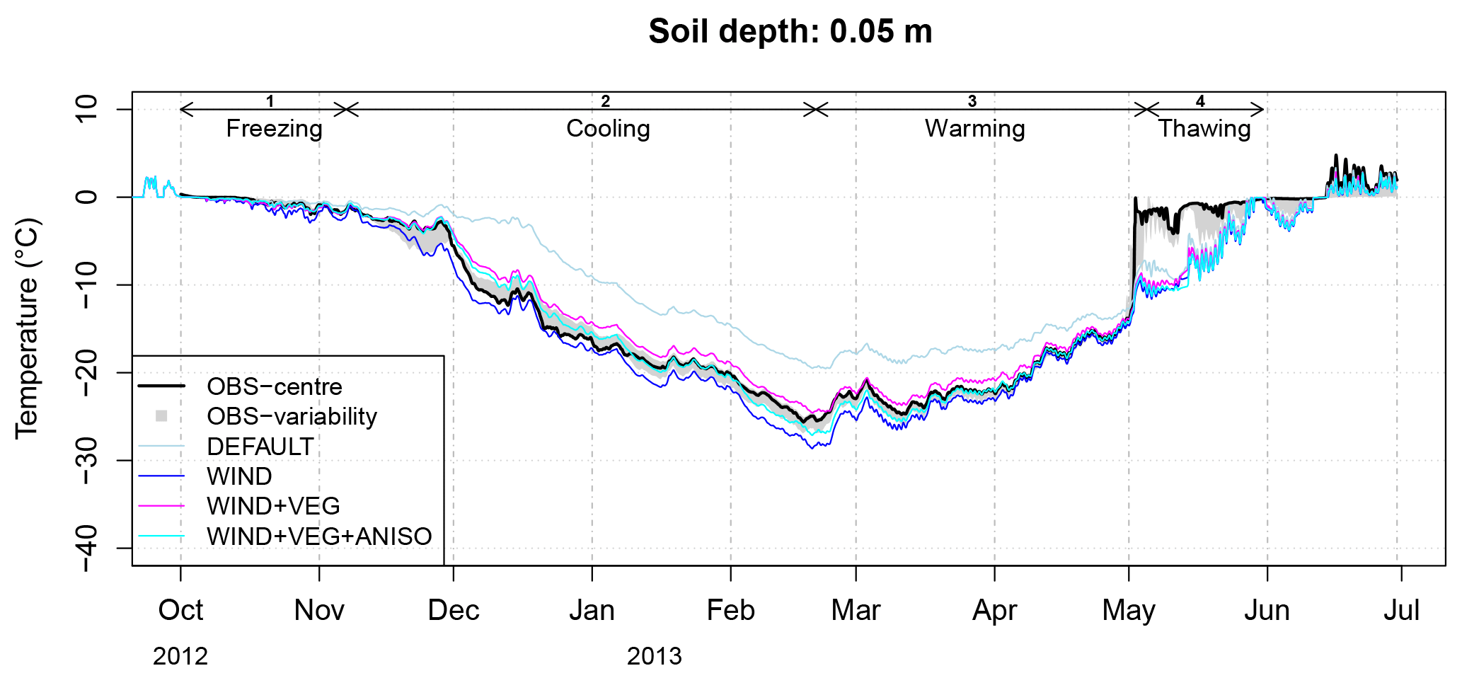
Figure 9As for Fig. 8 but with radiative transfer in snow switched off and the air layer scenario added to the WIND + VEG + ANISO option.
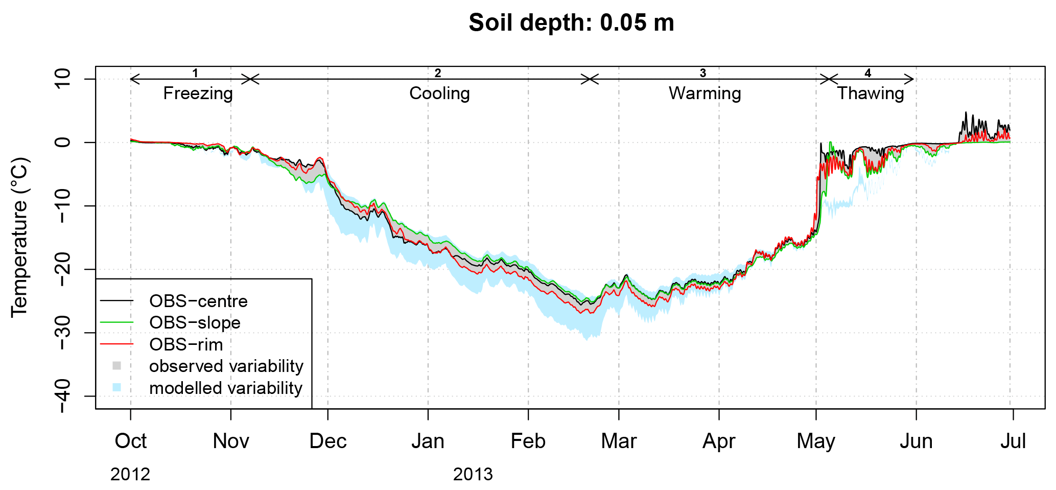
Figure 10Simulated and observed soil temperature variability (∘C) at 5 cm in depth. Observed soil temperatures at rim, centre, and slope locations in the reference polygon are overlain.
When driving CG3 simulations of the ground thermal regime, these 31 different snow insulation time series resulted in a pronounced spread of the simulated soil temperatures, which we refer to as “modelled variability” (Fig. 10). Comparison to soil temperature observations from the rim, slope, and centre revealed that the modelled variability encompasses the observed variability in soil temperature (Fig. 10), which is a desirable feature. However, the modelled variability is much higher than the observed one, especially during the cooling phase when it reaches 6.3 ∘C at 5 cm in depth while the observed one does not exceed 2 ∘C. For different reasons, it is likely that the rim, slope, and grass-centre soil temperature observations captured only part of the thermal impact of snow spatial variability at Samoylov: first, because of the small sample size (only three observations); second, due to a possible lack of representativity of the snow conditions on top of the soil sensors (they were not co-located with the CT samples, and snow was not characterized on top of them to avoid destruction of the snowpack); and third, because these soil temperature observations are also affected by spatial variability in the soil's thermal properties, which may interfere with any thermal effect solely due to snow variability. Additionally, lateral heat fluxes tend to smooth out any spatial variability in soil temperature, and they are not represented in our modelling. Finally, we also noticed that the measured rim and slope temperatures, which determine the maximum amplitude of the spread in the observations, responded differently at the beginning of the cooling phase, with the temperature dropping rapidly for the slope profile in early November but only gradually for the rim profile. This behaviour reversed from early December until the end of the cooling phase, with the spread in observed temperatures between a colder rim and a warmer slope reaching its maximum. The contrasting behaviour of rim and slope in November can be explained by several processes (e.g. contrasted early-season wind erosion–deposition, differences in the late autumn soil water content affecting the zero-curtain duration, and soil cooling dynamics) which are not captured by our modelling and may have limited the magnitude of the spread in observed temperatures.
During the warming period the variabilities in both modelled and observed soil temperatures are considerably reduced. Warming from the air is more efficient at sites with little snow insulation, which exhibit the coldest soil temperatures during the cooling phase, than at sites with a higher snow insulation. This explains the reduction in the spread of soil temperatures after the month of April. However, the reduction in the spread of simulated and observed soil temperatures starts earlier, in late February. This again indicates a reduced sensitivity of the ground thermal regime to variations in the thermal properties of the overlying snow during the whole warming phase (see the sensitivity experiment with the insertion of a basal air layer in Sect. 5.2). This reduced sensitivity will be analysed in Sect. 7 below.
Finally, our more thorough assessment of the spatial variability in soil temperatures here provides increased confidence to disqualify the simulations from the DEFAULT SNOWPACK set-up: this set-up was rejected in Sect. 5 as yielding soil temperatures that were too far above the observed range. Despite a spread in simulated soil temperatures larger than in the observations, our conclusion regarding the DEFAULT set-up remains unchanged as it yields soil temperatures also beyond the range of the simulated ones.
7.1 Comparison with snow data from similar contexts
The Samoylov snowpack shows similarities in its stratigraphy with Arctic snowpacks described previously by Domine et al. (2015, 2016b) and Derksen et al. (2009). The tundra snowpacks investigated by these authors along a sub-Arctic traverse comprised on average 65 % DH and had a mean density of 319 kg m−3. Both of these values are close to those from Samoylov (54 % and 279 kg m−3). The minor differences are probably due to differences in the wind conditions and the specific microtopography of Samoylov, where some samples were collected from wind-sheltered slope and centre sites or over frozen ponds. Derksen et al. (2009) also investigated the differences between snowpacks overlying lake ice, river ice, and tundra sites, identifying larger proportions of DH over ice, which is contrary to our own results. However, their study considered lake or river ice overlying liquid water that is warmer than the surrounding soil. This thermal contrast enhances the development of faceted grains. In contrast, the end-of-summer water level at the sampled ice-centre site at Samoylov was shallow, and shortly after freezing the ice extended to the ground, so that there could not be any enhanced thermal contrast created by an underlying relatively warm body of liquid water.
There are few published observations or reports on the thermal properties of Arctic tundra snow. To our knowledge, the Samoylov samples are among the first samples of tundra snow to be analysed by CT. Publications by Domine et al. (2015, 2016a, b) and Barrere et al. (2017), which relied on NP measurements and a refined retrieval algorithm for Keff, probably provide the most extensive thermal characterization of Arctic and sub-Arctic snowpacks in recent years. These authors reported values of Keff lower than our Keff−z estimates, both for DH layers and for the bulk snowpack. Barrere et al. (2017) measured Keff values no higher than 0.12 W m−1 K−1 for basal DH in the May 2014 and 2015 snowpacks at Bylot Island (Baffin Island, Canada); they however reported much higher conductivities (0.37 W m−1 K−1) for indurated DH. After correcting for a 20 % systematic error associated with the NP method, these authors calculated bulk Keff values of less than 0.1 W m−1 K−1 for the 2014 and 2015 Bylot snowpacks, resulting in highly insulating snow (bulk Rth values of 2.6 and 5.8 m2 K W−1). We estimated a bulk Rth of 0.87 m2 K W−1 for our CT grass-centre profile and a high upper bound of 1.59 m2 K W−1 for the CT slope profile. The Rth values obtained by Barrere et al. (2017) indicate insulation that is closer to the end-of-season insulation simulated by the DEFAULT set-up in SNOWPACK (Rth=1.75 m2 K W−1 in April 2013). This set-up led to an overestimation of February soil temperatures at Samoylov by about 6 ∘C. Such a bias can hardly be explained by the spatial variability in snow conditions (see Sect. 6). Despite the disagreement with published estimates for Keff under similar conditions, the consistency of the CT estimates for Keff−z with recent parameterizations and with measured soil temperatures after combined snow–soil modelling provides some confidence in them. The Samoylov snowpack appears more conductive than the 2013–2014 and 2014–2015 snowpacks observed at Bylot Island. Furthermore, our results compare very well with the conductivities obtained using inverse modelling by Jafarov et al. (2014) at Deadhorse (Alaska), a site with snow and meteorological conditions similar to Samoylov.
We estimate that the ground temperature spread induced solely by snow spatial variability can reach 6.3 ∘C in the coldest part of the winter at Samoylov (Sect. 6). This estimate is consistent with those in previous publications: Sturm and Holmgren (1994) observed maximum differences in ground surface temperatures of up to 19.1 ∘C and mean winter temperature differences of up to 7.2 ∘C, between the tops and hollows of grass tussocks at Imnavait Creek, Alaska. Their investigations focused on smaller-scale microrelief (tenths of a centimetre) than ours, resulting from grass tussocks in the tussock tundra. Our study complements the sensitivity study by Zhang et al. (1996), who found a 12.6 ∘C spread in winter ground surface temperatures following an increase in the proportion of DH from 0 % to 60 % at West Dock near Prudhoe Bay, Alaska. This study included neither an observation-based range of the proportions of DH in the snowpack nor the effect of co-varying DH thickness and snow depth. Furthermore, the DH and wind crust properties were kept constant over time. More recently, Gisnås et al. (2016) found a variability in ground temperatures of up to 6 ∘C in the Norwegian mountains, as a result of spatial variations in snow depth.
7.2 Light penetration in the Samoylov snowpack
The penetration of solar radiation in the natural snowpack at Samoylov is likely to be reduced by wind-blown sediments within some of the snow layers (Boike et al., 2003) and by the dense wind crusts at the top of the snowpack (Libois, 2014). While absorption of solar light in these layers may result in a localized increase in temperature within the snowpack, it is unlikely to have much warming effect on the underlying snow and soil because of the insulating nature of the snow. Brun et al. (2011) had to reduce the penetration depth of solar radiation in the CROCUS snow model in the same way that we did, in order to reproduce the snow temperatures at depths greater than 20 cm within the Antarctic snowpack at Dome C (Eric Brun, personal communication, 2011). Libois (2014) modelled a temperature reduction of ∼7 ∘C at 20 cm depth in the Dome C snowpack in summer as a result of spatial variations in density between 150 and 300 kg m−3 and consequent reduction in the penetration depth of solar radiation. Although radiative transfer models with fine spectral resolution that are able to circumvent this bias exist (Libois et al., 2013; Libois, 2014), these complex schemes are not implemented by default in operational snow models, which tends to hinder a proper representation of the underlying snow and soil thermal regime.
7.3 Temporal variations in the soil thermal sensitivity to snow properties
A key result of our ensemble simulations and observations is the increase in spatial variability in soil temperatures during the winter cooling phase and its reduction during the warming phase (Fig. 10). We ascribe this behaviour to two physical mechanisms. First, winter cooling is characterized by very steep temperature gradients between atmosphere and soil (about 150 K m−1; see Fig. C1 in Appendix C), which are later reduced and eventually vanish during the course of the warming phase. From Fourier's law for vertical heat flux (q)
it is apparent that the sensitivity of the heat flux to Keff−z is the temperature gradient. The greatest impact of spatial variations in Keff−z on ground temperatures is therefore expected to occur when temperature gradients are at a maximum (i.e. during the cooling phase), while a far smaller impact is expected when temperature gradients are low (i.e. during the warming phase).
Second, the reduction in the temperature gradient during the warming phase allows the soil temperatures to equilibrate laterally. At locations with more conductive snowpacks (e.g. polygon rims) the soil responds more rapidly to warming air, which further reduces the difference among these soil temperatures and those in more insulated locations (e.g. polygon slopes): this also contributes to the reduction in spatial variability in soil temperatures during the warming phase.
7.4 Limitations of our approach and perspectives
In Arctic snowpacks the water vapour flux induced by the steep temperature gradients redistributes ice mass from basal to upper snow layers, so that the density of the basal layers may actually decrease unless there is compensation through moisture flux from the soil. On the basis of Eq. (7) in Riche and Schneebeli (2013) and snow temperatures simulated with the WIND + VEG and WIND + VEG + ANISO options, we estimate that about 2 kg m−2 of ice is redistributed at Samoylov by this process between October and March. Unless sustained by soil water, this flux could lead to a 1.3 cm thick ice-depleted layer at the base of the snowpack (assuming a basal density of 150 kg m−3). The magnitudes of soil and snow vapour fluxes are not currently well constrained by observations, and they are not represented in detailed snow models such as SNOWPACK or CROCUS. To bypass these shortcomings and still produce reasonable SNOWPACK simulations, we adopted a phenomenological parameterization for the combined effects of snow vapour flux and vegetation on basal snow porosity. On the one hand, our adaptations to SNOWPACK are inherently local, tied to the specific Samoylov conditions and should be verified at other tundra sites comprising co-located snow and soil observations together with a complete set of meteorological driving data. On the other hand, neither this approach nor the current observational datasets allow the retrieval of any dynamics in basal snow ice depletion. A considerable uncertainty therefore remains regarding the thermal properties of snow in the early winter (cooling) period, when the sensitivity of ground thermal regimes to snow conditions is at its maximum. This uncertainty, together with uncertainty in the meteorological forcing that cannot be completely excluded, also affects our estimates of the thermal impact of snow spatial variability. Continuous monitoring of ice depletion at the base of the snowpack, and snow monitoring programs focusing on the early and dark winter periods at well-instrumented sites (see above), would help to provide better constraints for the thermal characteristics of the snowpack and the underlying metamorphic processes at this time, yielding substantial benefits for the next generation of coupled snow–soil models.
It also appears indispensable to include a more systematic and comprehensive treatment of anisotropy in snow models than the coarse diagnostic based on grain size and type that we have used, with a consistent link among water vapour flux, temperature gradient metamorphism, and anisotropy and with feedbacks on the mechanical (Srivastava et al., 2016), thermal, and optical properties of the snow. A promising way to further assess the relevance of anisotropy to the conductivity and the ground thermal regime may be to incorporate remote-sensing observations. It has been recently demonstrated (Leinss et al., 2016) that the depth-averaged anisotropy parameter (Q) of a snowpack can be estimated from polarimetric radar data such as, for example, those available from the TerraSAR-X satellite. Such an analysis could be used to produce global maps of the average anisotropy of snowpacks, as an indication of their metamorphic state.
Our combined SNOWPACK and CG3 simulations show a cold bias during and after melt-out. Hydrological processes within the snowpack related to thaw and rain are known to have an important influence on soil thermal dynamics, as has been emphasized in a large number of publications (e.g. Marsh and Woo, 1984a, b; Putkonen and Roe, 2003; Westermann, 2010). In naturally stratified snowpacks, water percolation and the associated heat transfer during early melt periods occur in part through “flow fingers”, which are preferential infiltration paths through the snow cover that penetrate into the colder substrata (snow layers or soil), where they refreeze, releasing latent heat (Marsh and Woo, 1984a, b). This process is known to delay the bulk melting of the snowpack, while at the same time accelerating soil warming. Progress has recently been made in the representation of preferential flow features by applying the Richards equation to water flow within a snow matrix (Wever et al., 2015; D'Amboise et al., 2017), but their impact on soil temperatures has not yet been assessed. Snow schemes used in permafrost models such as CG3 do not currently represent these processes, inducing significant biases in the melt period.
Finally, we assessed the impact of snow spatial variability linked to microtopography on the ground thermal regime. Our approach disregards the spatial variability in soil properties and soil saturation, which is also related to microtopography, as well as the lateral heat fluxes among different landscape units. Distributed three-dimensional simulations that include the effect of snow redistribution by wind and spatial variations in soil conditions could, in theory, support a more consistent assessment of spatial variability in soil temperatures. However, they require a considerable number of in situ data that are currently unavailable even at the most instrumented sites (Kumar et al., 2016). Models that have lower degrees of complexity but inherently account for spatial variability in snow and soil conditions within a statistical framework (e.g. Gisnås et al., 2016) provide a promising alternative and will benefit from the enhanced understanding that we have achieved of the links between microtopography and snow insulation.
Mixing in situ observations, cold laboratory analysis, and modelling, our work contributed to an improved characterization and understanding of the properties and spatial variability in an Arctic polygonal tundra snowpack and its role in shaping the underlying permafrost thermal regime during winter. Snow depth, which showed a strong correlation with microtopographical features, was found to be a crucial driver of the insulating power of snow over vegetated surfaces. The proportion of DH in the snowpack, which showed a weaker correlation with microtopography, introduced a second-order control. Waterlogged polygon centres in which basal ice forms during winter, were an exception to this rule of thumb due to weak DH formation resulting in conductive snowpacks despite intermediate snow depths.
The CT technique allowed estimates to be made of the thermal conductivity and anisotropy of Arctic snow samples that were mainly of DH and wind slabs with RGs. The retrieved properties confirmed the validity of a recent anisotropy and density-based parameterization of Keff−z, which had not previously been tested on Arctic snow samples. A comparison with other regressions for Keff−z highlighted the importance of taking anisotropy into account in Keff−z formulations, especially for DH.
Phenomenological adaptations of the SNOWPACK snow model to the Samoylov conditions, related to wind densification and the combined effect of basal vegetation and strong water vapour flux in the lower snowpack, enabled the simulation of snow density and Keff−z profiles in good agreement with our CT estimates. Introducing anisotropy considerations in the formulation of Keff−z used in the model resulted in further improvements. These adaptations jointly allowed improved simulations of the soil temperatures, providing further support for the soundness of our CT estimates for Keff−z.
We also estimated the impact of the natural snowpack spatial variability on the underlying permafrost thermal regime during an entire winter, based on our Keff−z and density observations and on our understanding of the snowpack dynamics. Beyond this quantitative estimate, which is intrinsically tied to the local climatology and microtopography of our site, an important conclusion is that the sensitivity of the ground thermal regime to the overlying snow reaches a maximum during the cooling winter period, when temperature gradients between atmosphere and soil are at their steepest. It is therefore crucial to better constrain the thermal properties of snow and the relevant processes during the first half of the winter, a period that is often less well monitored due to the dark and harsh winter conditions.
Finally, our study pinpointed processes that exert an important control on the ground thermal regime of tundra regions while being neglected in the snow schemes of general circulation models or Earth system models (e.g. Wang et al., 2013): the effect of wind compaction and DH growth on the insulating power of tundra snow, as well as the enhanced extinction of solar radiations by dense wind crusts within the snowpack. This suggests possible ways to improve snow representation over the Arctic regions in these models, of benefit for permafrost-related processes.
The adaptations to SNOWPACK used in this study are not included in the SNOWPACK distribution but the description provided in the paper allows the simulations to be reproduced in their entirety.
Meteorological and snow depth data are available at https://doi.org/10.1594/PANGAEA.879341 (Boike, 2017).
Regression of Q to optical diameter in data from Löwe et al. (2013)
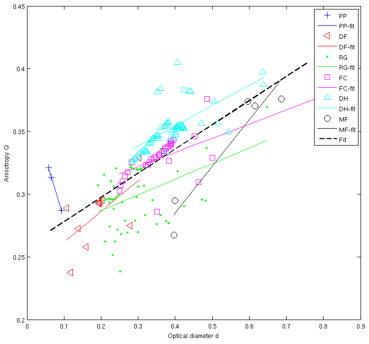
Figure A1Regression of anisotropy parameter Q to optical diameter d within snow type classes in data from Löwe et al. (2013).
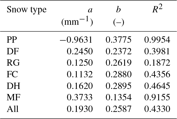
Table A1Regression coefficients for Fig. A1. All data within a snow type class were fitted to , where d is given in millimetres. When several grain types coexist, the dominant type is listed first.
Regression of Q to SNOWPACK grain radius, used in the ANISO adaptation
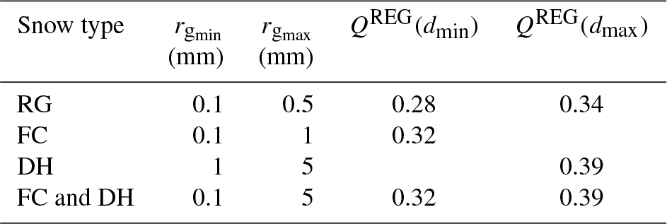
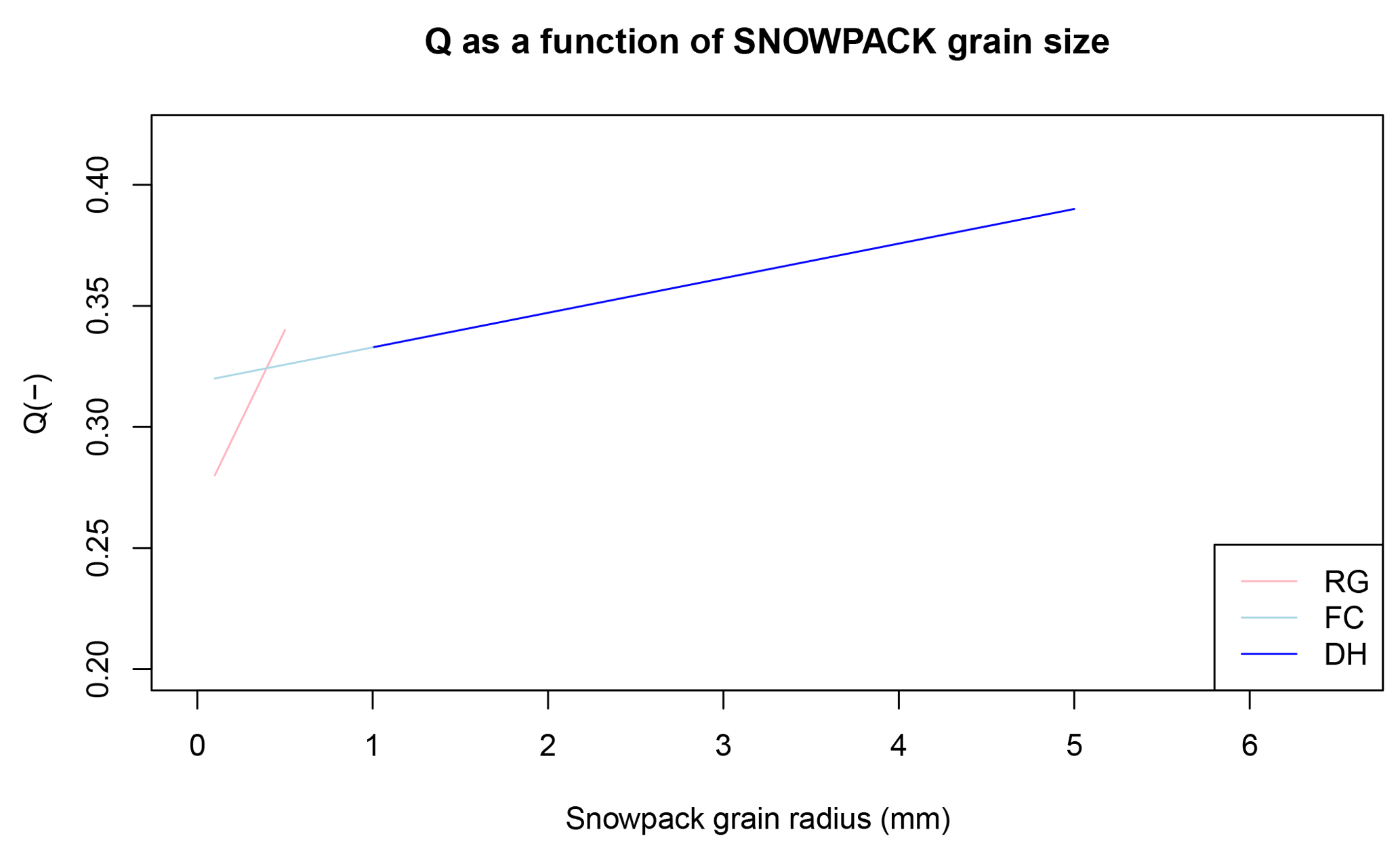
In the ANISO adaptation, Q is parameterized as a function (QANISO) of SNOWPACK grain radius (rg) for each of the FC, DH, and RG snow type classes:
where and are the maximum and minimum values of rg possibly achieved in SNOWPACK for the given snow type class (see Table A2), and dmax and dmin are the maximum and minimum values of d obtained in the data from Löwe et al. (2013) in the given snow type class.
Because SNOWPACK features a continuum between FC and DH grain radii, both grain type classes were merged in the ANISO adaptation by using QREG(dmax) from DH and QREG(dmin) from FC in Eq. (A1) (see Fig. A2).
A visual estimate of the DH thickness and total snow depth was made at each of the 31 transect points (pt), based on the NIR image from the date t2= 20 April 2013 (estimated accuracy ±0.5 cm).
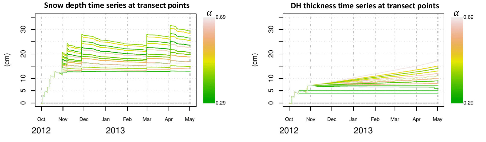
Figure B1Constructed snow depth and DH thickness time series for each transect point. As in the paper, α is the DH thickness-to-total snow depth ratio at time t2.
The following assumptions were made in the construction of DH thickness and snow depth (HS(t)) time series over the entire snow season consistent with observations made at the date t2.
-
The snow depth was assumed to build up in a spatially homogeneous manner until the date t1= 31 October (confirmed by time-lapse photographs of the reference polygon). All 31 data points were therefore attributed the same snow depth until that date (i.e. the corrected snow depth (HS50(t) measured by the SR50 sensor). Erosion–deposition processes subsequently led to different accumulations (HSpt) at each point along the transect. Do to the shortage of data, we linearly scaled HS50(t), which matched the end-of-season snow depth (HSpt(t2)) for each point:
-
We also considered a homogeneous DH build-up until t1: we used the DH build-up from the WIND + VEG + ANISO simulation for all transect points until t1. For t>t1, we considered the DH thickness at each transect point to increase linearly to its end-of-season value. An exception was made when the observed end-of-season DH thickness was less than the modelled DH thickness at t1: in this case we considered the DH thickness to remain constant after its end-of-season value had been reached in the SNOWPACK simulation.
The constructed snow depth and DH thickness time series are illustrated in Fig. B1.
Applying the two-layer approach to the snow depths and DH thickness time series using the snow properties described in the text (Sect. 6) leads to the Keff−z and Rth ensembles illustrated in Fig. B2.
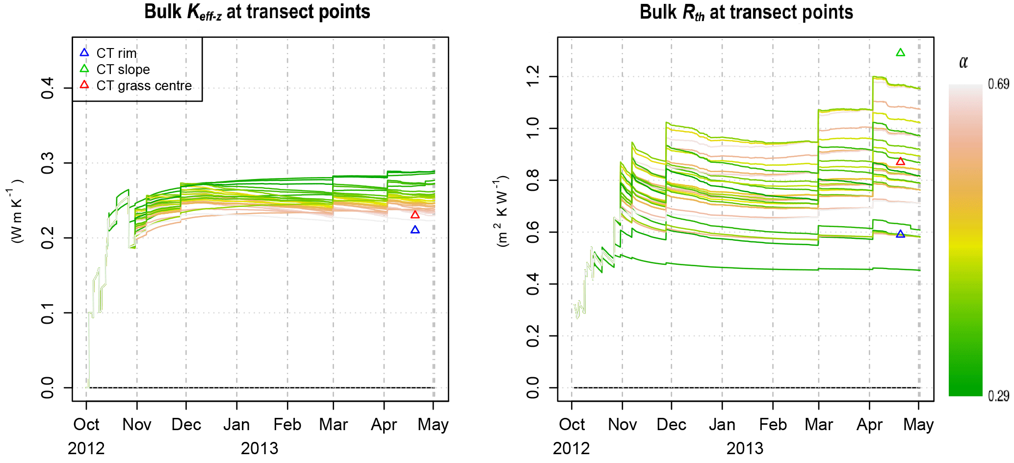
Figure B2Simulated Keff−z and Rth time series at the 31 transect data points. Overlain are the bulk properties estimated at the rim, slope, and grass-centre CT sites.
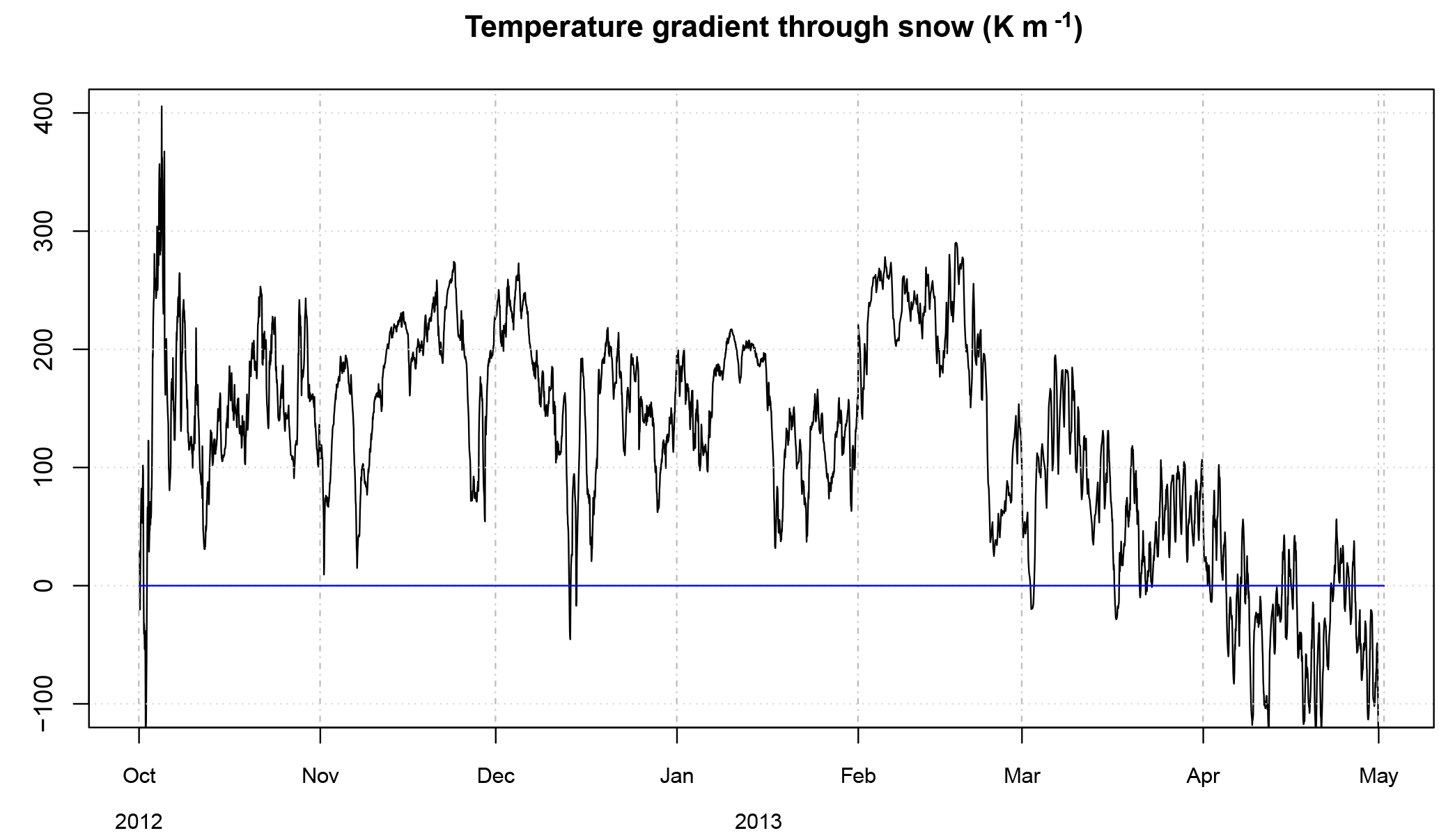
Figure C1Temperature gradient between air and soil (5 cm in depth) at the grass centre of the reference polygon.
MS and MP conceived the snow study. MP collected the snow data. ML and JB contributed the soil, permafrost, and meteorological measurements. IG, ML, and HL performed the numerical simulations. All authors contributed to the conception of the study. IG prepared the paper with contributions from all co-authors.
The authors declare that they have no conflict of interest.
This article is part of the special issue ”Changing Permafrost in the Arctic and its Global Effects in the 21st Century (PAGE21) (BG/ESSD/GMD/TC inter-journal SI)”. It is associated with a talk entitled “Snow observation and modeling for polygonal tundra permafrost thermal assessment”, presented at the POLAR2018 Conference, Davos, Switzerland, 19–23 June 2018.
We thank Mathias Bavay for his constant help and brilliant management of the
SNOWPACK core structure and integration of new developments. Our sincere
thanks go also to Michael Lehning and Charles Fierz for providing funding,
enthusiasm, and insightful comments on development choices. We thank Florent
Dominé for his vision of the relevant processes and the critical model
limitations and Jean-Emmanuel Sicart for very valuable comments. Finally, we
thank Franziska Gerber for deep scrutiny of the Samoylov meteorological
dataset. The field work for Martin Proksch was supported by the INTERACT-TA
project SSTIS.
Edited by: Christian Hauck
Reviewed by: two anonymous referees
Adams, E. E. and Sato, A.: Model for effective thermal conductivity of a dry snow cover composed of uniform ice spheres, Ann. Glaciol., 18, 300–304, 1993.
Avis, C. A., Weaver, A. J., and Meissner, K. J.: Reduction in areal extent of high-latitude wetlands in response to permafrost thaw, Nat. Geosci., 4, 444–448, 2011.
Barrere, M., Domine, F., Decharme, B., Morin, S., Vionnet, V., and Lafaysse, M.: Evaluating the performance of coupled snow–soil models in SURFEXv8 to simulate the permafrost thermal regime at a high Arctic site, Geosci. Model Dev., 10, 3461–3479, https://doi.org/10.5194/gmd-10-3461-2017, 2017.
Bartelt, P. and Lehning, M.: A physical SNOWPACK model for the Swiss avalanche warning: Part I: numerical model, Cold Reg. Sci. Technol., 35, 123–145, 2002.
Boike, J., Hinzman, L. D., Overduin, P. P., Romanovsky, V., Ippisch, O., and Roth, K.: A comparison of snow melt at three circumpolar sites: Spitsbergen, Siberia, Alaska, Proceedings of the 8th International Conference on Permafrost, Zurich, Switzerland, 21–25 July 2003, 79–84, 2003.
Boike, J., Wille, C., and Abnizova, A.: Climatology and summer energy and water balance of polygonal tundra in the Lena River Delta, Siberia, J. Geophys. Res., 113, G03025, https://doi.org/10.1029/2007JG000540, 2008.
Boike, J., Kattenstroth, B., Abramova, K., Bornemann, N., Chetverova, A., Fedorova, I., Fröb, K., Grigoriev, M., Grüber, M., Kutzbach, L., Langer, M., Minke, M., Muster, S., Piel, K., Pfeiffer, E.-M., Stoof, G., Westermann, S., Wischnewski, K., Wille, C., and Hubberten, H.-W.: Baseline characteristics of climate, permafrost and land cover from a new permafrost observatory in the Lena River Delta, Siberia (1998–2011), Biogeosciences, 10, 2105–2128, https://doi.org/10.5194/bg-10-2105-2013, 2013.
Boike, J.: Hourly meteorology and snow height at Samoylov met-station (2012-08-01–2013-06-30), Alfred Wegener Institute – Research Unit Potsdam, PANGAEA, https://doi.org/10.1594/PANGAEA.879341, 2017.
Brun, E., Six, D., Picard, G., Vionnet, V., Arnaud, L., Bazile, E., Boone, A., Bouchard, A., Genthon, C., Guidard, V., Le Moigne, P., Rabier, F., and Seity, Y.: Snow/atmosphere coupled simulation at Dome C, Antarctica, J. Glaciol., 57, 721–736, 2011.
Brun, E., Vionnet, V., Boone, A., Decharme, B., Peings, Y., Valette, R., Karbou, F., and Morin, S.: Simulation of northern eurasian local snow depth, mass, and density using a detailed snowpack model and meteorological reanalyses, J. Hydrometeorol., 14, 203–219, 2013.
Burke, E. J., Hartley, I. P., and Jones, C. D.: Uncertainties in the global temperature change caused by carbon release from permafrost thawing, The Cryosphere, 6, 1063–1076, https://doi.org/10.5194/tc-6-1063-2012, 2012.
Calonne, N., Flin, F., Morin, S., Lesaffre, B., du Roscoat, S. R., and Geindreau, C.: Numerical and experimental investigations of the effective thermal conductivity of snow, Geophys. Res. Lett., 38, L23501, https://doi.org/10.1029/2011GL049234, 2011.
Calonne, N., Flin, F., Geindreau, C., Lesaffre, B., and Rolland du Roscoat, S.: Study of a temperature gradient metamorphism of snow from 3-D images: time evolution of microstructures, physical properties and their associated anisotropy, The Cryosphere, 8, 2255–2274, https://doi.org/10.5194/tc-8-2255-2014, 2014.
Coléou, C., Lesaffre, B., Brzoska, J. B., Ludwig, W., and Boller, E.: Three-dimensional snow images by X-ray microtomography, Ann. Glaciol., 32, 75–81, 2001.
Dall'Amico, M., Endrizzi, S., Gruber, S., and Rigon, R.: A robust and energy-conserving model of freezing variably-saturated soil, The Cryosphere, 5, 469–484, https://doi.org/10.5194/tc-5-469-2011, 2011.
D'Amboise, C. J. L., Müller, K., Oxarango, L., Morin, S., and Schuler, T. V.: Implementation of a physically based water percolation routine in the Crocus/SURFEX (V7.3) snowpack model, Geosci. Model Dev., 10, 3547–3566, https://doi.org/10.5194/gmd-10-3547-2017, 2017.
Dee, D. P., Uppala, S. M., Simmons, A. J., Berrisford, P., Poli, P., Kobayashi, S., Andrae, U., Balmaseda, M.-A., Balsamo, G., Bauer, P., Bechtold, P., Beljaars, A. C. M., van de Berg, L., Bidlot, J., Bormann, N., Delsol, C., Dragani, R., Fuentes, M., Geer, A. J., Haimberger, L., Healy, S. B., Hersbach, H., Hólm, E. V., Isaksena, L., Kållberg, P., Köhler, M., Matricardi, M., McNally, A.-P., Monge-Sanz, B. M., Morcrette, J.-J., Park, B.-K., Peubey, C., de Rosnay, P., Tavolato, C., Thépaut, J. N., and Vitart, F.: The ERA-Interim reanalysis: Configuration and performance of the data assimilation system, Q. J. Roy. Meteor. Soc., 137, 553–597, 2011.
Derksen, C., Silis, A., Sturm, M., Holmgren, J., Liston, G. E., Huntington, H., and Solie, D.: Northwest Territories and Nunavut snow characteristics from a subarctic traverse: Implications for passive microwave remote sensing, J. Hydrometeorol., 10, 448–463, 2009.
Domine, F., Barrere, M., Sarrazin, D., Morin, S., and Arnaud, L.: Automatic monitoring of the effective thermal conductivity of snow in a low-Arctic shrub tundra, The Cryosphere, 9, 1265–1276, https://doi.org/10.5194/tc-9-1265-2015, 2015.
Domine, F., Barrere, M., and Morin, S.: The growth of shrubs on high Arctic tundra at Bylot Island: impact on snow physical properties and permafrost thermal regime, Biogeosciences, 13, 6471–6486, https://doi.org/10.5194/bg-13-6471-2016, 2016a.
Domine, F., Barrere, M., and Sarrazin, D.: Seasonal evolution of the effective thermal conductivity of the snow and the soil in high Arctic herb tundra at Bylot Island, Canada, The Cryosphere, 10, 2573–2588, https://doi.org/10.5194/tc-10-2573-2016, 2016b.
Fierz, C., Armstrong, R. L., Durand, Y., Etchevers, P., Greene, E., McClung, D. M., Nishimura, K., Satyawali, P. K., and Sokratov, S. A.: The international classification for seasonal snow on the ground, IHP-VII Technical Documents in Hydrology No 83, IACS Contribut ion No 1, UNESCO-IHP, Paris, France, 2009.
Garboczi, E. J.: Finite Element and Finite Difference Programs for Computing the Linear Electric and Elastic Properties of Digital Images of Random Materials, National Institute of Standards and Technology (NIST), Internal Report 6269, 1998.
Gisnås, K., Westermann, S., Schuler, T. V., Melvold, K., and Etzelmüller, B.: Small-scale variation of snow in a regional permafrost model, The Cryosphere, 10, 1201–1215, https://doi.org/10.5194/tc-10-1201-2016, 2016.
Gouttevin, I., Menegoz, M., Dominé, F., Krinner, G., Koven, C., Ciais, P., Tarnocai, C., and Boike, J.: How the insulating properties of snow affect soil carbon distribution in the continental pan-Arctic area, J. Geophys. Res., 117, G02020, https://doi.org/10.1029/2011JG001916, 2012.
Groot Zwaaftink, C. D., Cagnati, A., Crepaz, A., Fierz, C., Macelloni, G., Valt, M., and Lehning, M.: Event-driven deposition of snow on the Antarctic Plateau: analyzing field measurements with SNOWPACK, The Cryosphere, 7, 333–347, https://doi.org/10.5194/tc-7-333-2013, 2013.
Grosse, G., Goetz, S., McGuire, A. D., Romanovsky, V. E., and Schuur, E. A., Changing permafrost in a warming world and feedbacks to the Earth system, Environ. Res. Lett., 11, 040201 https://doi.org/10.1088/1748-9326/11/4/040201, 2016.
Heggli, M., Frei, E., and Schneebeli, M.: Snow replica method for three-dimensional X-ray microtomographic imaging, J. Glaciol., 55, 631–639, 2009.
Hobbie, S. E., Schimel, J. P., Trumbore, S. E., and Randerson, J. R.: Controls over carbon storage and turnover in high-latitude soils, Glob. Change Biol., 6, 196–210, https://doi.org/10.1046/j.1365-2486.2000.06021.x, 2000.
Hutchison, B. A.: Snow accumulation and disappearance influenced by big sagebrush, Research Note RM 46, Rocky Mountain Forest and Range Experiment Station, Forest Service, US Department of Agriculture, Fort Collins, USA, 1965.
Jafarov, E. E., Nicolsky, D. J., Romanovsky, V. E., Walsh, J. E., Panda, S. K., and Serreze, M. C.: The effect of snow: How to better model ground surface temperatures, Cold Reg. Sci. Technol., 102, 63–77, 2014.
Koven, C., Friedlingstein, P., Ciais, P., Khvorostyanov, D., Krinner, G., and Tarnocai, C.: On the formation of high-latitude soil carbon stocks: Effects of cryoturbation and insulation by organic matter in a land surface model, Geophys. Res. Lett., 36, L21501, https://doi.org/10.1029/2009GL040150, 2009.
Kumar, J., Collier, N., Bisht, G., Mills, R. T., Thornton, P. E., Iversen, C. M., and Romanovsky, V.: Modeling the spatiotemporal variability in subsurface thermal regimes across a low-relief polygonal tundra landscape, The Cryosphere, 10, 2241–2274, https://doi.org/10.5194/tc-10-2241-2016, 2016.
Langer, M., Westermann, S., Heikenfeld, M., Dorn, W., and Boike, J.: Satellite-based modeling of permafrost temperatures in a tundra lowland landscape, Remote Sens. Environ., 135, 12–24, 2013.
Langer, M., Westermann, S., Boike, J., Kirillin, G., Grosse, G., Peng, S., and Krinner, G.: Rapid degradation of permafrost underneath waterbodies in tundra landscapes: Toward a representation of thermokarst in land surface models, J. Geophys. Res.-Earth, 121, 2446–2470, 2016.
Lawrence, D. M. and Slater, A. G.: The contribution of snow condition trends to future ground climate, Clim. Dynam., 34, 969–981, 2010.
Lehning, M. and Fierz, C.: Assessment of snow transport in avalanche terrain, Cold Reg. Sci. Technol., 51, 240–252, 2008.
Lehning, M., Bartelt, P., Brown, B., and Fierz, C.: A physical SNOWPACK model for the Swiss avalanche warning: Part III: Meteorological forcing, thin layer formation and evaluation, Cold Reg. Sci. Technol., 35, 169–184, 2002a.
Lehning, M., Bartelt, P., Brown, B., Fierz, C., and Satyawali, P.: A physical SNOWPACK model for the Swiss avalanche warning: Part II. Snow microstructure, Cold Reg. Sci. Technol., 35, 147–167, 2002b.
Leinss, S., Löwe, H., Proksch, M., Lemmetyinen, J., Wiesmann, A., and Hajnsek, I.: Anisotropy of seasonal snow measured by polarimetric phase differences in radar time series, The Cryosphere, 10, 1771–1797, https://doi.org/10.5194/tc-10-1771-2016, 2016.
Libois, Q.: Evolution des propriétés physiques de neige de surface sur le plateau Antarctique. Observations et modélisation du transfert radiatif et du métamorphisme, PhD thesis, Université Grenoble Alpes, France, 273 pp., 2014.
Libois, Q., Picard, G., France, J. L., Arnaud, L., Dumont, M., Carmagnola, C. M., and King, M. D.: Influence of grain shape on light penetration in snow, The Cryosphere, 7, 1803–1818, https://doi.org/10.5194/tc-7-1803-2013, 2013.
Liljedahl, A. K., Boike, J., Daanen, R. P., Fedorov, A. N., Frost, G. V., Grosse, G., Hinzman, L. D., Iijma, Y., Jorgenson, J. C., Matveyeva, N., Necsoiu, M., Raynolds, M. K., Romanovsky, V. E., Schulla, J., Tape, K. D., Walker, D. A., Wilson, C. J., Yabuki, H., and Zona, D.: Pan-Arctic ice-wedge degradation in warming permafrost and its influence on tundra hydrology, Nat. Geosci., 9, 312–318, 2016.
Liston, G. E. and Elder, K.: A distributed snow-evolution modeling system (SnowModel), J. Hydrometeorol., 7, 1259–1276, https://doi.org/10.1175/JHM548.1, 2006.
Löwe, H., Riche, F., and Schneebeli, M.: A general treatment of snow microstructure exemplified by an improved relation for thermal conductivity, The Cryosphere, 7, 1473–1480, https://doi.org/10.5194/tc-7-1473-2013, 2013.
Marsh, P. and Woo, M. K.: Wetting front advance and freezing of meltwater within a snow cover: 1. Observations in the Canadian Arctic, Water Resour. Res., 20, 1853–1864, 1984a.
Marsh, P. and Woo, M. K.: Wetting front advance and freezing of meltwater within a snow cover: 2. A simulation model, Water Resour. Res., 20, 1865–1874, 1984b.
Montpetit, B., Royer, A., Roy, A., Langlois, A., and Derksen, C.: Snow microwave emission modeling of ice lenses within a snowpack using the microwave emission model for layered snowpacks, IEEE T. Geosci. Remote, 51, 4705–4717, 2013.
Muster, S., Langer, M., Heim, B., Westermann, S., and Boike, J.: Subpixel heterogeneity of ice-wedge polygonal tundra: a multi-scale analysis of land cover and evapotranspiration in the Lena River Delta, Siberia, Tellus B, 64, 17301, https://doi.org/10.3402/tellusb.v64i0.17301, 2012.
Muster, S., Heim, B., Abnizova, A., and Boike, J.: Water body distributions across scales: A remote sensing based comparison of three arctic tundra wetlands, Remote Sensing, 5, 1498–1523, 2013.
Nash, J. E. and Sutcliffe, J. V.: River flow forecasting through conceptual models part I – A discussion of principles, J. Hydrol., 10, 282–290, 1970.
O'Neill, A. D. J. and Gray, D. M: Solar radiation penetration through snow, in: The Role of Snow and Ice in Hydrology, Proceedings of the Banff Symposium, Banff, Canada, September 1972, 227–240, 1972.
Ouellet, F., Langlois, A., Blukacz-Richards, E. A., Johnson, C. A., Royer, A., Neave, E., and Larter, N. C.: Spatialization of the SNOWPACK snow model for the Canadian Arctic to assess Peary caribou winter grazing conditions, Phys. Geogr., 38, 143–158, 2017.
Putkonen, J. and Roe, G.: Rain-on-snow events impact soil temperatures and affect ungulate survival, Geophys. Res. Lett., 30, 1188, https://doi.org/10.1029/2002GL016326, 2003.
Riche, F. and Schneebeli, M.: Thermal conductivity of snow measured by three independent methods and anisotropy considerations, The Cryosphere, 7, 217–227, https://doi.org/10.5194/tc-7-217-2013, 2013.
Rutter, N., Sandells, M., Derksen, C., Toose, P., Royer, A., Montpetit, B., Langlois, A., Lemmetyinen, J., and Pulliainen, J.: Snow stratigraphic heterogeneity within ground-based passive microwave radiometer footprints: Implications for emission modelling, J. Geophys. Res.-Earth, 119, 550–565, 2014.
Schneebeli, M. and Sokratov, S. A.: Tomography of temperature gradient metamorphism of snow and associated changes in heat conductivity, Hydrol. Process., 18, 3655–3665, 2004.
Schneider, C. A., Rasband, W. S., and Eliceiri, K. W.: NIH Image to ImageJ: 25 years of image analysis, Nat. Methods, 9, 671–675, 2012
Schuur, E. A. G., McGuire, A. D., Schädel, C., Grosse, G., Harden, J. W., Hayes, D. J., Hugelius, G., Koven, C. D., Kuhry, P., Lawrence, D. M., Natali, S. M., Olefeldt, D., Romanovsky, V. E., Schaefer, K., Turetsky, M. R., Treat, C. C., and Vonk, J. E.: Climate change and the permafrost carbon feedback, Nature, 520, 171–179, 2015.
Srivastava, P. K., Chandel, C., Mahajan, P., and Pankaj, P.: Prediction of anisotropic elastic properties of snow from its microstructure, Cold Reg. Sci. Technol., 125, 85–100, 2016.
Sturm, M. and Benson, C. S.: Vapor transport, grain growth and depth-hoar development in the subarctic snow, J. Glaciol., 43, 42–59, 1997.
Sturm, M. and Holmgren, J.: Effects of microtopography on texture, temperature and heat flow in Arctic and sub-Arctic snow, Ann. Glaciol., 19, 63–68, 1994.
Sturm, M. and Johnson, J. B.: Thermal conductivity measurements of depth hoar, J. Geophys. Res., 97, 2129–2139, 1992.
Sturm, M., Holmgren, J., König, M., and Morris, K.: The thermal conductivity of seasonal snow, J. Glaciol., 43, 26–41, 1997.
Vionnet, V., Brun, E., Morin, S., Boone, A., Faroux, S., Le Moigne, P., Martin, E., and Willemet, J.-M.: The detailed snowpack scheme Crocus and its implementation in SURFEX v7.2, Geosci. Model Dev., 5, 773–791, https://doi.org/10.5194/gmd-5-773-2012, 2012.
Wainwright, H. M., Liljedahl, A. K., Dafflon, B., Ulrich, C., Peterson, J. E., Gusmeroli, A., and Hubbard, S. S.: Mapping snow depth within a tundra ecosystem using multiscale observations and Bayesian methods, The Cryosphere, 11, 857–875, https://doi.org/10.5194/tc-11-857-2017, 2017.
Waite, W. F., Gilbert, L. Y., Winters, W. J., and Mason, D. H.: Estimating thermal diffusivity and specific heat from needle probe thermal conductivity data, Rev. Sci. Instrum., 77, 044904, https://doi.org/10.1063/1.2194481, 2006.
Wang, T., Ottlé, C., Boone, A., Ciais, P., Brun, E., Morin, S., Krinner, G., Piao, S., and Peng, S.: Evaluation of an improved intermediate complexity snow scheme in the ORCHIDEE land surface model, J. Geophys. Res.-Atmos., 118, 6064–6079, 2013.
Westermann, S.: Sensitivity of permafrost, PhD thesis, Ruperto-Carola University of Heidelberg, Germany, 192 pp., 2010.
Westermann, S., Langer, M., Boike, J., Heikenfeld, M., Peter, M., Etzelmüller, B., and Krinner, G.: Simulating the thermal regime and thaw processes of ice-rich permafrost ground with the land-surface model CryoGrid 3, Geosci. Model Dev., 9, 523–546, https://doi.org/10.5194/gmd-9-523-2016, 2016.
Wever, N., Schmid, L., Heilig, A., Eisen, O., Fierz, C., and Lehning, M.: Verification of the multi-layer SNOWPACK model with different water transport schemes, The Cryosphere, 9, 2271–2293, https://doi.org/10.5194/tc-9-2271-2015, 2015.
Yen, Y. C.: Review of thermal properties of snow, ice and sea ice, CRREL Report 81-10, CRREL, Hannover, New-Hampshire, 1981.
Zhang, T.: Influence of the seasonal snow cover on the ground thermal regime: An overview, Rev. Geophys., 43, RG4002, https://doi.org/10.1029/2004RG000157, 2005.
Zhang, T., Osterkamp, T. E., and Stamnes, K.: Influence of the depth hoar layer of the seasonal snow cover on the ground thermal regime, Water Resour. Res., 32, 2075–2086, 1996.
Zhang, T., Barry, R., Knowles, K., Heginbottom, J., and Brown, J.: Statistics and characteristics of permafrost and ground-ice distribution in the Northern Hemisphere, Polar Geography, 31, 47–68, 2008.
- Abstract
- Introduction
- Data and methods
- Thermal properties of the Samoylov snowpack
- Adaptations of the SNOWPACK model to the Arctic context at Samoylov
- Simulations of snow properties and ground thermal regime (grass-centre site)
- Thermal implications of snow spatial variability
- Discussion
- Conclusion
- Code availability
- Data availability
- Regression of anisotropy parameter Q to grain size
- Construction of snow depth, DH height, Keff−z, and Rth time series at the transect data points
- Appendix C: Thermal gradient between air and soil (5 cm depth)
- Author contributions
- Competing interests
- Special issue statement
- Acknowledgements
- References