Glacio-hydrological melt and run-off modelling: application of a limits of acceptability framework for model comparison and selection

Glacio-hydrological models (GHMs) allow us to develop an understanding of how future climate change will affect river flow regimes in glaciated watersheds. A variety of simplified GHM structures and parameterisations exist, yet the performance of these are rarely quantified at the process level or with metrics beyond global summary statistics. A fuller understanding of the deficiencies in competing model structures and parameterisations and the ability of models to simulate physical processes require performance metrics utilising the full range of uncertainty information within input observations. Here, the glacio-hydrological characteristics of the Virkisá River basin in southern Iceland are characterised using 33 signatures derived from observations of ice melt, snow coverage and river discharge. The uncertainty of each set of observations is harnessed to define the limits of acceptability (LOA), a set of criteria used to objectively evaluate the acceptability of different GHM structures and parameterisations. This framework is used to compare and diagnose deficiencies in three melt and three run-off-routing model structures. Increased model complexity is shown to improve acceptability when evaluated against specific signatures but does not always result in better consistency across all signatures, emphasising the difficulty in appropriate model selection and the need for multi-model prediction approaches to account for model selection uncertainty. Melt and run-off-routing structures demonstrate a hierarchy of influence on river discharge signatures with melt model structure having the most influence on discharge hydrograph seasonality and run-off-routing structure on shorter-timescale discharge events. None of the tested GHM structural configurations returned acceptable simulations across the full population of signatures. The framework outlined here provides a comprehensive and rigorous assessment tool for evaluating the acceptability of different GHM process hypotheses. Future melt and run-off model forecasts should seek to diagnose structural model deficiencies and evaluate diagnostic signatures of system behaviour using a LOA framework.

1 Introduction

Computational GHMs allow us to develop an understanding of how future climate change will affect river flow regimes in glaciated watersheds (Lutz et al., 2014; Radić and Hock, 2014; Ragettli et al., 2016; Singh et al., 2016; Teutschbein et al., 2015). A variety of GHM codes exist (Boscarello et al., 2014; Ciarapica and Todini, 2002; Huss et al., 2008b; Lindström et al., 1997; Schaefli et al., 2014; Schulla, 2015), each of which includes a number of model components that represent two broad groups of processes: (i) glaciological mass balance, the accumulation and ablation of snow and ice; and (ii) hydrological water balance, the storage and release of melt and rainfall through snow, ice, overland and the subsurface. The exact form that these model components should take, both in terms of their governing equations (structure) and numerical constants (parameterisation) is not known. Physically based models which solve equations derived from first principles, typically over a distributed grid, are our closest approximation of the “true” structure. However, limited parameterisation data and computer resources often preclude the use of such complex models, particularly in remote mountainous regions where data are scarce and where the inclusion of extra complexity does not guarantee better predictions (Gabbi et al., 2014).

Simplified process models offer an alternative. They are faster to run and employ fewer parameters, which are typically calibrated to available observation data. They are based on, but do not necessarily adhere to, physical laws and as such their mathematical structure is somewhat unconstrained and may be biased towards a particular scientist's own perceptions and understanding of environmental processes. This has led to the development of a variety of competing model structures which purport to simulate the same process, but which have been derived from different process hypotheses. For example, a number of simplified index model structures of snowmelt and ice melt exist. The classical temperature index model (TIM) simulates melt as a linear piecewise function of temperature only (Braithwaite, 1995), a hypothesis that can be justified because of the influence temperature has on the total energy balance of ice and snow, particularly in temperate climates (Aðalgeirsdóttir et al., 2011; Guðmundsson et al., 2009; Ohmura, 2001). So-called “enhanced” TIM structures have also been proposed, which include added levels of complexity with the purpose of providing more accurate estimates of melt. These have accounted for perturbations in melt caused by topographic shading (Hock, 1999), surface albedo characteristics (Oerlemans, 2001; Pellicciotti et al., 2005) and debris cover (Carenzo et al., 2016).

Similarly a number of simplified representations of processes governing the hydrological water balance have been used in GHMs. Arguably, the equations that govern the routing (transport) of run-off are most important in relation to river flow predictions in glaciated river basins, as storage characteristics of ice and snow strongly influence river flow regimes over a range of timescales (Jansson et al., 2003). The concept of linear reservoirs is the most widely adopted simplified approach for run-off-routing in glaciated basins (Gao et al., 2017; Hanzer et al., 2016; Zhang et al., 2015). A linear reservoir lumps all of the interacting, non-linear and non-stationary components of water transmission within a predefined area (e.g. a watershed) into a single “leaky bucket”. Despite its simplicity, the linear reservoir has been shown to be remarkably versatile at capturing the storage–discharge characteristics of glaciated river basins around the world (Farinotti et al., 2012; Hock and Jansson, 2005; de Woul et al., 2006). This is partly because the concept lends itself to structural modifications that can represent different glacio-hydrological systems. Hanzer et al. (2016) hypothesised that the snowpack, firn layer, glacier ice and the region free from ice all exhibit unique run-off-discharge responses and advocate the use of four linear reservoirs in parallel to distinguish between these units. However, simpler structural configurations use only two linear reservoirs in parallel to route meltwater through the snowpack and ice separately (Hannah and Gurnell, 2001) or even a single linear reservoir to route all rainfall and melt run-off simultaneously (Boscarello et al., 2014), which can accurately reproduce river discharge time series.

The availability of multiple, presumably plausible, simplified model structures presents somewhat of a dilemma to glaciologists and hydrologists as they are left with some uncertainty about how processes should be represented in their models. For the purpose of river discharge predictions, this problem is particularly pertinent, as there are competing structures for two fundamental controls on these predictions: snowmelt and ice melt and run-off-routing. One approach to mitigate this is to determine the optimum structure that best captures the observation data. Structural optimisation of simplified run-off-routing routines has largely been ignored in glacio-hydrological contexts (Hannah and Gurnell, 2001), but more studies have sought to optimise and compare simplified models of melt. Gabbi et al. (2014) applied four different TIMs to Rhonegletscher, Switzerland. They found that all achieved a similar goodness-of-fit to 6 years of ablation stake data, but that the inclusion of a solar radiation term provided the most accurate predictions of multi-decadal measurements of ice volume change. Irvine-Fynn et al. (2014) applied six different TIMs to the high-Arctic Midtre Lovénbreen glacier but only found minor improvements in capturing seasonal ablation stake data when various levels of complexity were introduced to the classical (temperature-only) TIM. More recently, a comparison of four TIMs applied to four glaciers in the French Alps by Reveillet et al. (2017) found no clear evidence that using an enhanced TIM over the classical temperature-only approach provided better simulations when compared to a 17-year data set of ablation stake measurements. Mosier et al. (2016) used a multi-criterion evaluation approach to compare the performance of different conceptual melt model structures. They compared seven competing melt model structures in two glaciated catchments in Alaska to ablation stake, river discharge and remotely sensed snow coverage data. They found that no single model was best across all of the observation data sets, but the inclusion of a cold-content representation of snow consistently produced the best goodness-of-fit scores over the evaluation data.

Clearly, while some studies have provided useful insight into the comparative behaviour between competing conceptual process hypotheses (particularly for melt), none provide any definitive reasoning for adopting (or not) a particular model structure. Of course, discriminating between competing model structures in this way is made difficult by the fact that observation data used to drive and evaluate models are uncertain and therefore we cannot be sure whether model deficiencies represent inadequacies in the model or the data (Beven, 2016). Beven (2006) argues that, because of this uncertainty and because of the fact that all models are by definition imperfect, no one optimum model structure (or parameterisation) exists. Instead, there is an equifinality of behavioural models that make predictions within some predefined acceptability bounds around the observation data that take various sources of modelling uncertainty into account. Indeed, parameter equifinality is a well recognised phenomenon in conceptual models of snowmelt and ice melt (Finger et al., 2015; Gabbi et al., 2014; Jost et al., 2012; Pellicciotti et al., 2012; Reveillet et al., 2017). If we accept this, then the priority within the glacio-hydrological modelling community should be to establish frameworks that allow us to robustly evaluate model appropriateness and distinguish between behavioural (acceptable) and non-behavioural (unacceptable) structures and parameterisations. Constraining the range of acceptable models is particularly important for glacio-hydrological modelling, as it has been shown that model uncertainty can lead to high uncertainty in 21st century predictions of river flows in glaciated basins (Huss et al., 2014).

One potential source of inspiration is the hydrological rainfall-run-off modelling community. Their heavy reliance on an ever-expanding choice of conceptual hydrological process models to predict river flow prompted Gupta et al. (2008) to discuss the need for a better framework with which to discriminate between these competing process hypotheses. They focussed on the evaluation metrics and noted that there was an overreliance on metrics that quantify the average performance of a model (e.g. root mean squared error and Nash–Sutcliffe efficiency), which reduces information held in observation data down to a single summary statistic. They argue for a multi-criterion, diagnostic approach for which more of the relevant information from observation data is extracted so that inadequacies in model structures and parameterisations can be better identified. Rye et al. (2012) applied such an approach to optimise a distributed surface mass balance model of two glaciers in Svalbard. They used ablation stake data to define three different features of the observations including mass balance at the stake locations, long-term mass balance trend and mass balance gradient. Using a multi-objective optimisation procedure, they identified structural inadequacies relating to how the mass balance gradient was simulated.

Hydrologists are now moving away from traditional metrics of model performance in favour of more diagnostic signatures of hydrological behaviour. These have typically been derived from river flow time series and may be as simple as the mean flow (an indicator of water balance) or they can be used to characterise the distribution (e.g. flow percentiles) and the timing (e.g. autocorrelation) of flows. They have shown to have more discrimination power than traditional error metrics (Euser et al., 2013; Hrachowitz et al., 2014; Schaefli, 2016; Shafii and Tolson, 2015) and, importantly, it is also possible to take into account their information content (i.e. their uncertainty) so that decisions about model appropriateness can be made within the uncertainties of observation data used to evaluate the model. Here, observation data uncertainty can be used to define quantitative limits of acceptability (LOA) around each signature. Different model structures and parameterisations can then be systematically evaluated for their ability to capture the signatures within their LOA, allowing the modeller to objectively diagnose model deficiencies and make decisions about model appropriateness. The LOA framework has been used to constrain the parameters of a distributed hydrological model for flood prediction (Blazkova and Beven, 2009), evaluate the appropriateness of different hydrological model structures across contrasting geological settings (Coxon et al., 2014) and, most recently, to diagnose deficiencies in a hydrological model based on its ability to capture a range of river discharge signatures for an alpine catchment (Schaefli, 2016).

A signature-based approach within a LOA framework could also be used to compare and diagnose deficiencies in different simplified melt and run-off-routing model structures and parameterisations employed in GHMs. For this purpose, signatures need not be derived just from river discharge data but should also be taken from other observation sources such as ice melt and snow coverage, as these have shown to be useful for evaluating the consistency of GHMs across different aspects of glacio-hydrological systems (Finger et al., 2011, 2015; Hanzer et al., 2016; Mayr et al., 2013). By doing this, the framework could facilitate better predictions of river flow regime changes in glaciated river basins, firstly by helping to diagnose deficiencies in GHM structures that require improvement, and secondly, by objectively selecting the range of acceptable model structures and parameterisations so that prediction uncertainty can be better constrained.

This study is the first of its kind to apply a signature-based LOA framework for a multi-GHM-structure evaluation. The framework is used to evaluate three different melt model structures and three different run-off-routing model structures with the aim of investigating its utility for (i) diagnosing deficiencies in different model structures, indicating the framework's usefulness for aiding future improvement of simplified process models; and (ii) constraining a prior population of model structures and parameterisations down to a smaller population of acceptable models, indicating the framework's usefulness for reducing prediction uncertainty. To do this, the models were applied to the glaciated Virkisá River basin in southern Iceland where observation data were used to derive 33 signatures of ice melt, snow coverage and river discharge against which the models were calibrated and evaluated. LOA were defined around each signature so that acceptable and unacceptable model structures and parameterisations could be defined. The results were first used to evaluate the capacity of the different signatures for discriminating between acceptable and unacceptable model structures and parameterisations when used individually. They were then used to compare the acceptability of the different melt and run-off-routing model structures across the range of signatures.

2 Methodology

2.1 Study site

The Virkisá River basin covers an area of 22 km² on the western side of the ice-capped Öræfajökull stratovolcano in south-eastern Iceland (Fig. 1). It rises from near sea level to the west, where it is bounded by steep cliffs, up to an ice-filled caldera at the summit of Öræfajökull (∼ 2000 m a.s.l.), the edge of which forms the basin's uppermost boundary. The basin forms a major drainage channel for accumulated ice which flows in a south-westerly direction down the steeply sloped Öræfajökull (average slope of 0.25). It flows along two distinct glacier arms (Virkisjökull and Falljökull, hereafter referred to as Virkisjökull), around a bedrock ridge before meeting again at the terminus (∼ 150 m a.s.l.). Virkisjökull has a high mass balance gradient with a net annual accumulation of more than 7 m w.e. yr⁻¹ at the summit (Guðmundsson, 2000) and net annual ice melt of more than 8 m w.e. yr⁻¹ in the main ablation zone (Flett, 2016). It has been in a phase of retreat since 1990 due to warming of the climate over this period (Hannesdóttir et al., 2015). Since 2005 the rate of retreat has accelerated to > 30 m yr⁻¹ as a result of the detachment of the ice front from the active part of the glacier, resulting in rapid downwasting (Bradwell et al., 2013; IGS, 2017; Phillips et al., 2014). This recent rapid retreat has resulted in the formation of a small proglacial lake at the terminus which forms the headwater of the Virkisá River. The Virkisá River flows in a south-westerly direction, firstly through a 800 m bedrock-controlled section flanked on either side by push moraines from previous glacial advances. From here it continues to flow over an extensive and gently sloping sandur floodplain. The steep-sided valley walls and the relatively recent glacial maximum at the end of the Little Ice Age, circa 1890, mean that there is limited soil development in and around the Virkisá River basin. Where thin soils have developed, vegetation is dominated by mosses, sparse grass and shrubs such as dwarf willow and birch.

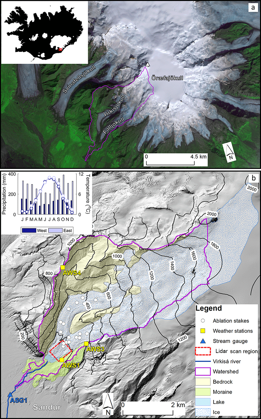
Figure 1 Location of Virkisá River basin on Öræfajökull (a) and detailed topographical map of the basin including major land surface types and observation data with inset showing mean monthly climate (b).

Long-term meteorological records from two weather stations operated by the Icelandic Meteorological Office 10 km east and west of the study site show that the region experiences a maritime climate characterised by cool summers (∼ 10 ^∘C on average) and mild winters (∼ 1 ^∘C on average) with year-round precipitation (see inset in Fig. 1b). The prevailing north-easterly wind and orographic lift over Öræfajökull induces a strong lateral precipitation gradient where more than 2 times the precipitation falls to the east (3500 mm yr⁻¹) of the river basin than to the west (1500 mm yr⁻¹). Near-surface air temperature is mainly controlled by the altitudinal variations over Öræfajökull where the average temperature lapse rate is −0.44 ^∘C 100 m⁻¹ (Flett, 2016).

2.2 Observation data

2.2.1 Climate

Several different sources of climate data are available for the study site. Measurements within the catchment are available from three automatic weather stations (AWSs) installed by the British Geological Survey (BGS) between 2009 and 2011 as part of their investigation into the retreat of the Virkisjökull glacier. These are situated at 156, 444 and 805 m a.s.l. (Fig. 1b) and they measure temperature, air pressure, humidity, wind speed and rainfall every 15 min. The lowest weather station (AWS1) is also equipped with a cosine-corrected pyranometer which measures incident short-wave radiation. None of the weather stations are designed to measure snowfall and therefore precipitation measurements during freezing temperatures are not available.

Two additional sources of climate data are available. Firstly, the Fagurhólsmýri weather station operated by the Icelandic Meteorological Office (IMO) approximately 12 km south of the study site has daily measurements of temperature dating back to 1949 and therefore provides long-term variations in temperature around the study region. The IMO has also recently produced a 2.5 km gridded data set of total precipitation as part of the ICRA atmospheric reanalysis project (Nawri et al., 2017). These data provide the best estimate of long-term precipitation at the study site and, given the limited availability of precipitation measurements at higher elevations around Öræfajökull, they also provide the best estimate of spatial variations in precipitation across the region.

2.2.2 Ice melt

An array of 17 ablation stakes installed by Flett (2016) in the main ablation zone of the glacier between 2012 and 2014 at elevations ranging from 142 to 462 m a.s.l. provide measurements of ice melt on the glacier tongue (Fig. 1b). The BGS have also undertaken annual high-resolution (sub-metre) terrestrial lidar scans of the proglacial region including ice at the front of the glacier (see red dashed box in Fig. 1b) which, given that ice flow is negligible here, provides an additional indication of ice melt.

Two digital elevation models of the ice also exist for the years 1988 and 2011, which indicate the historical retreat of Virkisjökull. A 5 m 2011 DEM was constructed using high-resolution airborne lidar scans of the ice surface (IMO, 2013) and is considered the most accurate measurement of the ice geometry and surrounding topography in the study region currently available. A 20 m 1988 DEM was derived from aerial photographs of the glacier (Landmælingar Íslands: https://www.lmi.is/, last access: 1 October 2017) using photogrammetric methods (Magnússon et al., 2016). Photogrammetry may suffer from errors due to image rectification and stereo-image mismatches (Barrand et al., 2009) and therefore the accuracy of this data set is expected to be less certain, particularly over higher-elevation snow-covered terrain.

2.2.3 Snow coverage

No direct observations of snow accumulation or melt exist for the Virkisá River basin and so, instead, satellite snow cover data (MOD10A1 product) from the Moderate Resolution Imaging Spectroradiometer (MODIS) (Riggs and Hall, 2015) were used. These data have been archived since 2000 and consist of daily 500 m gridded maps of snow cover extent with values ranging between 0 and 1 which relate to the proportion of the ground that is snow covered. While they do not provide a direct measurement of snow mass balance, they have shown to be a useful data source for evaluating the performance of GHMs (Finger et al., 2015; Hanzer et al., 2016). The quality of the data in high-latitude regions such as Iceland are variable due to the need for good light and little or no cloud cover. As part of the MOD10A1 product, a basic estimate of the data quality is calculated as a means to avoid measurements affected by cloud cover and poor light conditions. For this study, only those data that achieved a QA score of “good” or “best” were used. This precluded the use of data collected between September and February, presumably because of reduced daylight hours and increased cloud cover during these months.

2.2.4 River discharge

Hourly river discharge data collected since 2012 are available from an automatic stream gauge installed by the BGS 2 km downstream of the lake outlet on the Virkisá River (see ASG1 in Fig. 1). The gauge consists of two stilling wells with submerged pressure transducers which measure river stage and water temperature every 15 min. The stage data are subsequently converted into units of flow using a rating curve constructed from periodic river flow gaugings.

In conjunction with the river stage and water temperature measurements, a camera is mounted next to the river and takes photos of the channel 3 times a day. Given that the river is prone to freezing over the winter months, the photographic archive and temperature data were used to remove these periods from the river flow time series. The river bed consists of large boulders (approximate diameter of 50 cm) which can become mobile during high flows, causing shifts in the rating curve. For this study, river discharge data for the years 2013 and 2014 were used because gaugings for these years cover a wide range of flow magnitudes and rating shifts are limited and well constrained by observations.

2.3 Glacio-hydrological model

A distributed GHM, which can incorporate different conceptual representations of melt and run-off-routing processes, was used for all model experiments. The code was written in the object-oriented C$++$ programming language, making it computationally efficient and ideally suited for incorporating different model structures. The GHM consists of a 2-D Cartesian grid of equally spaced model nodes. For this study, a spatial resolution of 50 m was selected as the best balance between simulation detail and model performance. Hourly observations of precipitation, temperature and incident solar radiation were used to simulate the accumulation of snowfall and the melt of snow, firn and ice across the model domain. The snow redistribution algorithm developed by Huss et al. (2008a) was used to account for snow drift and avalanches based on the curvature and slope of the surface. A soil infiltration and evapotranspiration model developed by Griffiths et al. (2006) solves the water balance for the non-glaciated regions of the study catchment. Excess soil moisture, rainfall and melt are then routed to the catchment outlet via a semi-distributed network of linear-reservoir cascades which represent the water storage and release characteristics of the major hydrological pathways in the watershed. The GHM also simulates the evolution of the glacier geometry under periods of sustained negative mass balance using the Δh parametrisation of glacier retreat, which has been shown to closely reproduce the evolution of alpine glaciers with results comparable to more complex 3-D finite-element ice flow models (Huss et al., 2010). Details of this and the soil water balance component of the GHM can be found in Appendix A. The following text details the different melt and run-off-routing structures adopted for this study.

2.3.1 Snowmelt and ice melt model structures

Melt of snow and ice is calculated at each model node separately. Snowmelt can occur at any node where a snow pack has developed. Similarly, ice melt can only occur at ice-covered nodes where the snow pack has completely melted. The mass balance at a given node is the summation of snowfall minus snowmelt and ice melt. The GHM uses the mass balance calculated at each node to determine the equilibrium line altitude (ELA) which is updated each simulation year. A rolling 3-year average ELA was used to determine the dividing line between firn and ice on the glacier.

For this study, three different conceptual models of snowmelt and ice melt with different levels of complexity were compared. All have been used extensively to simulate melt processes in glaciated regions around the world (Gao et al., 2017; Matthews and Hodgkins, 2016; Nepal et al., 2017; Ragettli et al., 2016; Reveillet et al., 2017). The first melt model structure (TIM₁) employs a classic temperature index model approach (Braithwaite, 1995) whereby melt is assumed to increase linearly with temperature above a given critical threshold:

$$\begin{array}{}\text{(1)}& M_i=\left\{\begin{array}{ll}{a}_i(T-T_i^{*})& T>T_i^{*}\\ \mathrm{0}& T\le T_i^{*}\end{array}\right.,\end{array}$$

where a (m w.e. ^∘C⁻¹ h⁻¹) is the temperature factor calibration parameter that converts temperature into melt, T is the near-surface air temperature and T^* is the critical threshold above which melt occurs. To account for the different properties of snow, firn and ice that may bring about different values of a and T^*, these are defined separately so that i = (snow, firn, ice).

The second melt model structure (TIM₂) was originally proposed by Hock (1999) and includes an additional incident solar radiation term to account for topographic effects such as slope, aspect and shading which can bring about spatio-temporal variations in melt (Arnold et al., 2006; Pellicciotti et al., 2008). Their enhanced TIM has the form

$$\begin{array}{}\text{(2)}& M_i=\left\{\begin{array}{ll}(T-T_i^{*})(a_i+b_i\cdot {\text{SW}}_{\downarrow })& T>T_i^{*}\\ \mathrm{0}& T\le T_i^{*}\end{array}\right.,\end{array}$$

where b (m³ w.e. W^−1 ∘C⁻¹ h⁻¹) is an additional radiation factor calibration parameter that converts the measured incident solar radiation, SW_↓ (W m²) into a unit melt. For this melt model structure the GHM accounts for shading using the DEM and position of the sun in the sky, which is calculated for each hourly time step using the SPA algorithm (Reda and Andreas, 2008). Additional perturbations in solar irradiance at the surface brought about by topographic effects such as slope and aspect are accounted for by calculating the incident angle of solar radiation to scale the measured incoming radiation.

Konya et al. (2004) noted that the form of Eq. (2) is not congruent with the full energy balance equation, as temperature is used to multiply the short-wave radiation term, which can lead to overestimation of melt during peak temperatures. Accordingly the melt model structure proposed by Pellicciotti et al. (2005) was also used for this study (TIM₃), which is an enhanced TIM in additive form that also incorporates an albedo parameter, α:

$$\begin{array}{}\text{(3)}& M_i=\left\{\begin{array}{ll}{a}_i(T-T_i^{*})+b_i\cdot {\text{SW}}_{\downarrow }(\mathrm{1}-{\mathit{\alpha }}_i)& T>T_i^{*}\\ \mathrm{0}& T\le T_i^{*}\end{array}\right.,\end{array}$$

where b has the units m³ w.e. W⁻¹ h⁻¹. Following Pellicciotti et al. (2005), this melt model structure also includes the dynamic snow albedo algorithm proposed by Brock et al. (2000), which accounts for the drop in snow albedo as it ages using a logarithmic function with the form:

$$\begin{array}{}\text{(4)}& {\mathit{\alpha }}_{\text{snow}}=p_{\mathrm{1}}-p_{\mathrm{2}}\cdot {\log }_{\mathrm{10}}\cdot T_{\text{a}},\end{array}$$

where p₁ is the albedo of fresh snow (set to 0.9), p₂ is an empirical calibration parameter and T_a is the accumulated daily maximum temperature greater than 0 ^∘C since snowfall.

For all melt model structures in the GHM, melt M is converted into a volumetric melt M_v at each node:

$$\begin{array}{}\text{(5)}& M_{\text{v}}=M\cdot A,\end{array}$$

where A is the model node area. Following Hopkinson et al. (2010) the area of each node is corrected for surface slope:

$$\begin{array}{}\text{(6)}& A={\displaystyle \frac{L^{\mathrm{2}}}{\cos \mathit{\beta }}},\end{array}$$

where L is the model node length and β is the node surface slope.

2.3.2 Run-off-routing model structures

Run-off is generated by rainfall falling on snow and ice as well as snowmelt, ice melt and excess soil moisture from those areas free of ice and snow. The concept of linear reservoirs was employed to route this run-off to the catchment outlet. A linear reservoir receives a volumetric inflow and releases it at a rate proportional to its internal water storage following

$$\begin{array}{}\text{(7)}& q={\displaystyle \frac{\mathrm{1}}{k}}s,\end{array}$$

where q is the outflow (m³ h⁻¹), s is the storage (m³) and k is mean residence time of the reservoir (h), which accounts for the diffusive effect of storage and release mechanisms within the catchment. Increasing the value of k increases the diffusion effect on the inflow hydrograph. Additional controls on the diffusion and lag effects can be obtained by arranging a cascade of multiple linear reservoirs in series (Ponce, 2014) so that the outflow from the previous reservoir is the inflow to the subsequent reservoir. With this set-up, the continuity equation for the jth reservoir of n reservoirs in series, where $j=(\mathrm{1},\mathrm{2}\mathrm{\dots }n)$ can be written as

$$\begin{array}{}\text{(8)}& {\displaystyle \frac{\mathrm{d}{s}_j}{\mathrm{d}t}}=\left\{\begin{array}{ll}i-q_j& j=\mathrm{1}\\ q_{j-\mathrm{1}}-q_j& j>\mathrm{1}\end{array}\right..\end{array}$$

The outflow hydrograph is then taken from q_n.

For temperate glaciers, common practice is to subdivide the catchment into one or more hydrological response units (HRUs) which are thought to have different water storage and release characteristics. For example, the firn, snow and bare ice have generally been shown to respond over relatively long, intermediate and short timescales respectively (Hock and Jansson, 2005), and therefore these may be characterised as separate HRUs, although as noted previously, simpler and more complex definitions of HRUs have been defined in the past. Subsequently, three run-off-routing model structures were proposed with different levels of complexity structured around these subdivisions (Fig. 2).

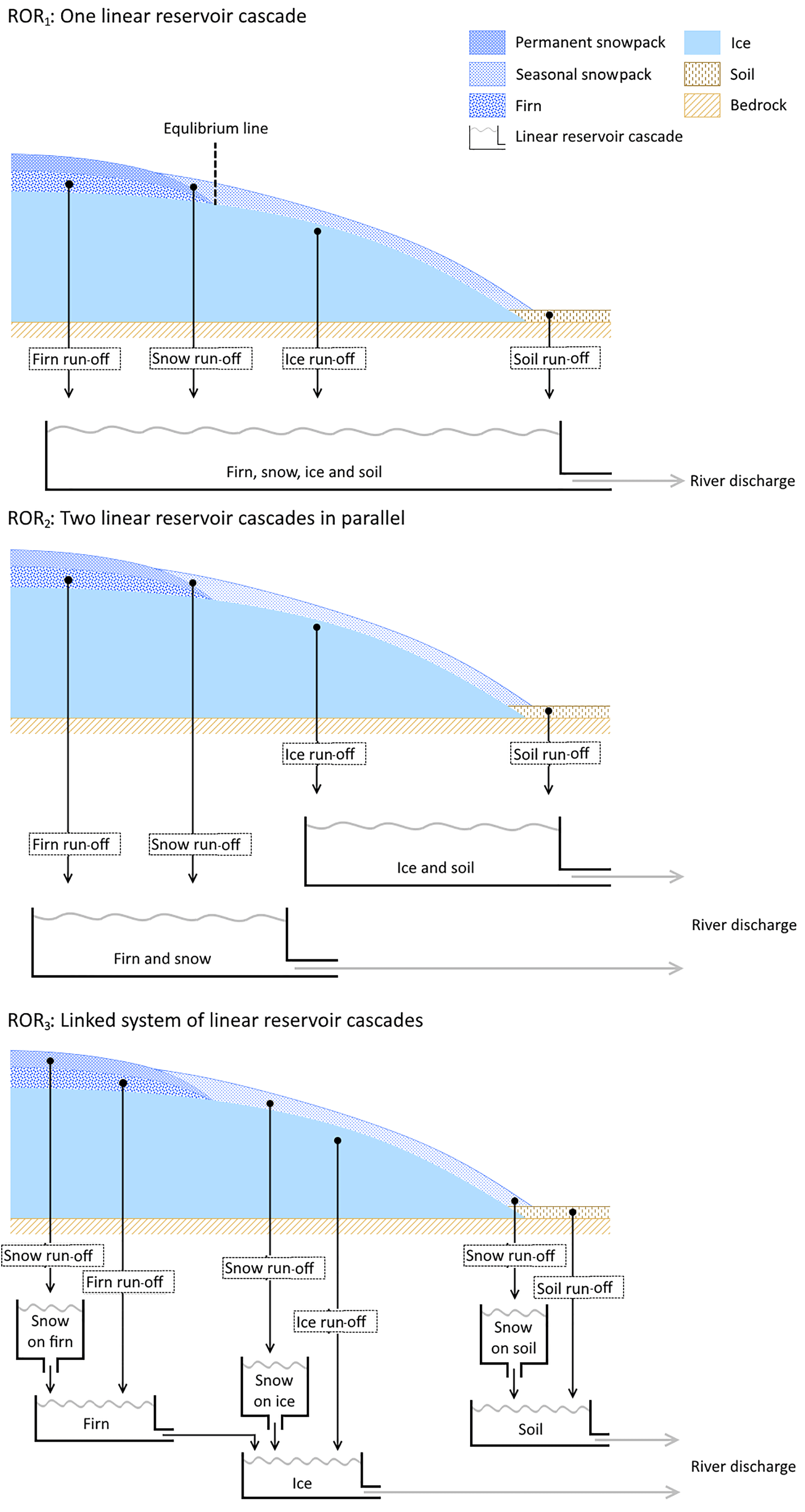
Figure 2 Three run-off-routing model structures which relate the linear reservoir cascade configurations to idealised cross sections of a temperate glacier.

The first and simplest run-off-routing model structure (ROR₁) uses a single linear reservoir cascade (Boscarello et al., 2014) to route the inflow from all run-off sources simultaneously. This structure makes no distinction between the different run-off sources and flow pathways and assumes that all conform to the same storage–discharge relationship.

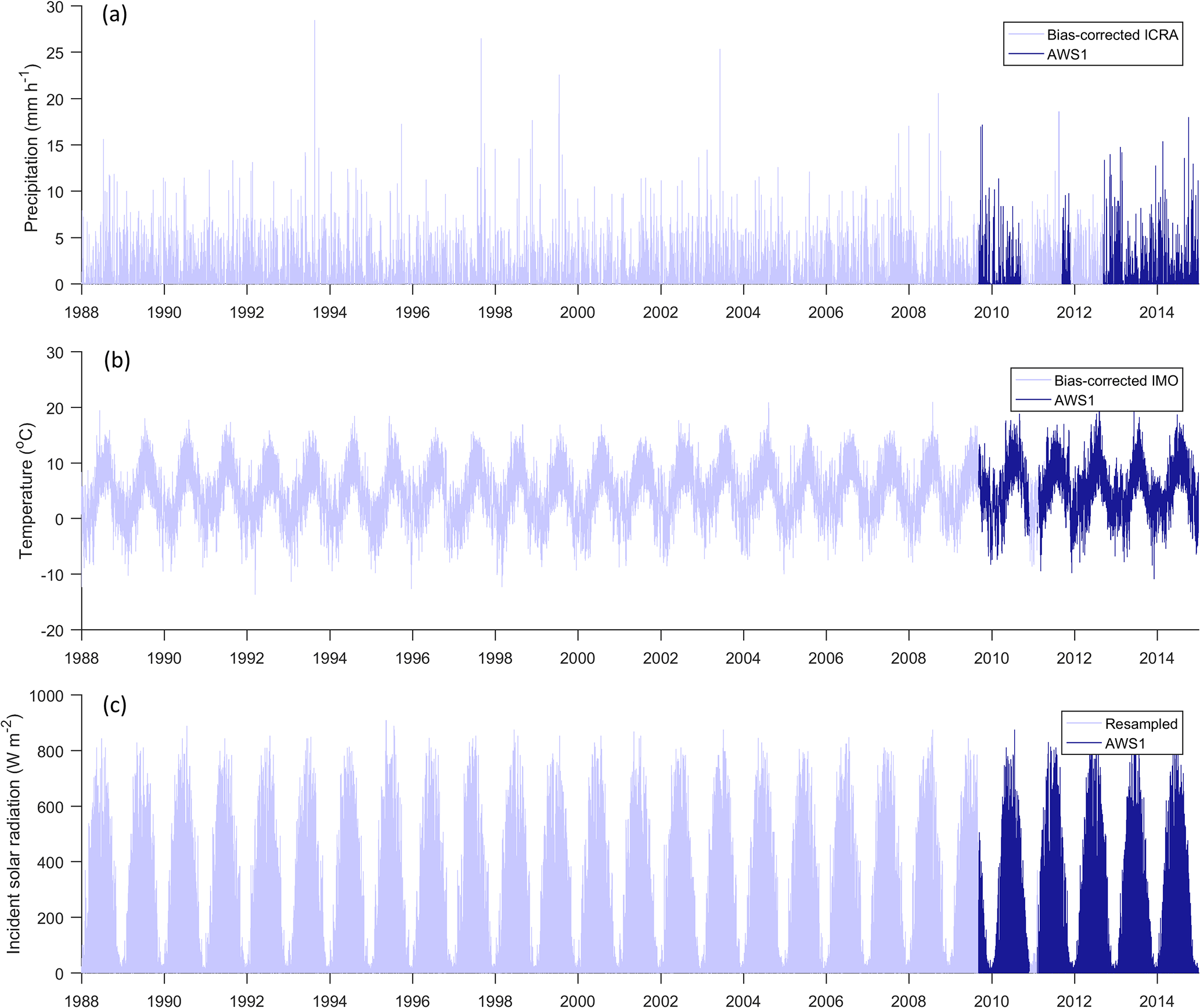
Figure 3 Continuous hourly time series of precipitation (a), temperature (b) and incident solar radiation (c) between 1988 and 2015 at AWS1.

The second model structure (ROR₂), employs two linear reservoir cascades in parallel (Hannah and Gurnell, 2001). The first cascade represents the slow percolation of water through the snow and firn HRUs, while the second cascade represents a faster flow of water through the bare ice and overland. This approach therefore makes some distinction between the different flow pathways and, by conditioning the parameters so that the snow and firn have a more diffuse response function, it introduces a degree of non-linearity in the discharge response to run-off.

The third run-off-routing model structure (ROR₃) has not been used previously. It employs separate linear reservoir cascades to route water from the firn, snow, ice and soil HRUs. Here the parameters are conditioned so that the firn is the most diffuse, slowly responding reservoir, followed by the snow, and then the ice and soil zones are considered to be relatively fast-responding HRUs. This approach also includes some representation of linkages between these various units. Here it is hypothesised that water that flows through the firn must then flow through the downstream bare ice HRU before it reaches the river. Similarly, water that percolates through the snow pack must also flow via the HRU that it overlies before it reaches the river. There are therefore six different flow pathways that run-off may take before reaching the river outlet (see Fig. 2c) and this represents the most complex, non-linear run-off-routing model structure.

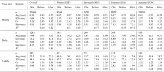
Table 1 Statistics calculated from the observed (Obs) precipitation data at AWS1 and from the corresponding ICRA precipitation data before and after bias correction. Statistics have been calculated at an hourly, daily and 3-daily time step and include n (total number of above-freezing measurements available at AWS1), avg (mean), SD (standard deviation), Cv (coefficient of variation), skewness and R² (coefficient of determination).

2.4 Driving climate data

The GHM was configured to run from the initial ice geometry of 1988 to 2015. It requires continuous measurements of hourly precipitation, near-surface air temperature and incident solar radiation to drive the various model components.

2.4.1 Precipitation

A new gridded precipitation time series was constructed for the GHM, which incorporates the measurements of rainfall from the weather stations in the Virkisá basin and the information on spatial and long-term variations in precipitation from the gridded ICRA reanalysis product. First, the weather station rainfall data were used to correct the ICRA reanalysis product for bias. Given that none of the weather stations are equipped with devices to measure snowfall, and that freezing temperatures can induce erroneous measurements in rainfall, only data with three consecutive preceding above-freezing days were used. This is a major issue when using AWS4, as the majority of days, particularly in the winter, are below freezing at this elevation. Accordingly, the AWS4 rainfall data were not used for the bias-correction procedure. Furthermore, because the AWS1 and AWS3 gauges overlap the same ICRA data pixel, and because the AWS1 time series is the longest and most complete, it was decided that the AWS1 data should be used to correct the overlapping ICRA data pixel. Here, the equidistant quantile mapping (EQM) approach (Li et al., 2010; Sachindra et al., 2014; Srivastav et al., 2014) was employed to correct the ICRA precipitation time series for bias. EQM is an adaptation of the original quantile mapping method that accounts for non-stationarity in the moments of the biased time series and helps to preserve changes in the cumulative distribution function of the precipitation data that may have occurred over time (Cannon et al., 2015; Switanek et al., 2017). To evaluate the effectiveness of the bias-correction procedure, a number of statistics were calculated to compare the observed and ICRA precipitation data before and after bias correction (Table 1). There were a total of 30 460 hourly measurements of precipitation available for above-freezing days at AWS1 of which the majority were during the autumn months (September, October and November) and the least during the winter months (December, January and February). Overall, the procedure corrects for bias in the mean (Avg) and also improves the spread (SD), relative variability (CV) and skewness of the distribution of precipitation data at hourly, daily and 3-daily time steps. On a seasonal scale, these improvements are notable for spring, summer and autumn. However, the bias-correction procedure typically has a slightly negative impact on the winter precipitation statistics, probably because of the limited above-freezing data available for these months. In particular, average hourly winter precipitation is underestimated by 0.11 mm (16 %), while the positive bias in relative variability and skewness are amplified after bias correction. Given that EQM preserves the rank correlation of the time series, it has little effect on the R² correlation score, with a typical reduction of 0.01–0.02 after bias correction. At an hourly timescale, the bias-corrected data only captured 22 % of the observed variance in the AWS1 rainfall record. However, when averaged to a daily time step the R² score increased to 0.49, and for a 3-daily time step the R² increased to 0.72. The limited correlation of the ICRA precipitation data on an hourly timescale could hinder the acceptability of the GHM across some of the signatures (e.g. the river discharge signatures related to the timing of flows). However, the AWS1 rainfall record is complete for the years 2013 and 2014 for which the GHM is compared against observed river discharge signatures. As such, poor replication of the timing of hourly rainfall events should have minimal influence on the GHM's ability to capture the river discharge signatures. Rather, the role of the bias-corrected ICRA precipitation data was primarily to drive the glacier mass balance component of the GHM prior to 2009 for which a reliable 3-daily temporal correlation with observations was deemed adequate.

2.4.2 Near-surface air temperature

The longest record of hourly temperature measurements in the Virkisá River basin are from AWS1, which starts in 2009. To generate a continuous time series of temperature back to 1988, daily measurements of temperature available from the nearby Fagurhólsmýri weather station were used. A comparison of daily average temperatures showed there to be a good linear relationship between the two stations with an R² of 0.92. As such, this linear model was used to correct the daily weather station data for bias so that it could be combined with the AWS1 time series. To downscale the data to an hourly resolution, 24 h temperature anomalies were randomly sampled from the AWS1 record, thereby ensuring the complete time series had a consistent subdaily variability. Of course, diurnal cycles in temperature are dependent on the time of year, in that increased incident solar radiation in the summer enhances subdaily temperature variability. Therefore, the sampling strategy was employed on a month-by-month basis. The complete hourly time series of temperature at AWS1 is shown in Fig. 3b.

As in many glaciated catchments topography controls spatial temperature variations to a large extent. The importance of characterising temperature lapse rates for glacio-hydrological modelling is well known because it strongly controls spatial patterns of melt simulations (Gardner and Sharp, 2009; Heynen et al., 2013; MacDougall et al., 2011). In fact, while many studies employ a fixed temperature lapse rate, in reality seasonal variations in surface characteristics (e.g. albedo and roughness) and atmospheric conditions can bring about strong seasonal and diurnal variations in lapse rates which control melt processes (Gardner et al., 2009; Immerzeel et al., 2014; Minder et al., 2010). Furthermore, local atmospheric phenomena associated with midlatitude glaciers, such as katabatic winds which bring cool dense air over the ice surface, can serve to reduce the temperature gradient (Petersen and Pellicciotti, 2011; Ragettli et al., 2014). Having analysed near-surface air temperature variations both on and away from the Virkisjökull glacier, it was deemed most appropriate to extrapolate temperature across the study catchment using a seasonally variable hourly lapse rate in conjunction with an on-ice temperature correction function based on the work of Shea and Moore (2010) (see Appendix B).

2.4.3 Incident solar radiation

The only source of incident solar radiation is the continuous hourly time series from AWS1. To construct a continuous time series back to 1988, a resampling strategy was employed to generate a complete time series that was statistically consistent with the data at AWS1. It was found that, during the summer months, the daily range in incident solar radiation and temperature are strongly correlated. Therefore, when generating a continuous time series of hourly incident solar radiation from 1988, it was important to maintain this dependence between intra-day solar radiation and temperature variability. To do this, a coordinated (in time) sampling strategy identical to that used for the near-surface air temperature data was employed. More specifically, for each random 24 h temperature anomaly sample from the AWS1 record used to build part of the temperature time series, the corresponding 24 h solar cycle data were extracted and used to build the same part of the incident solar radiation time series. Figure 3c shows the complete time series of incident solar radiation used to drive the model.

2.5 Signatures and limits of acceptability

Observations of ice melt, snow coverage and river discharge were used to derive 33 unique signatures with LOA to characterise the glacio-hydrological behaviour of the Virkisá River basin over different spatio-temporal scales and evaluate the acceptability of the different model structures (Table 2). For convenience, the signatures have also been subdivided into 11 attributes which encapsulate the main aspects of model behaviour that were assessed.

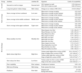
Table 2 Summary of signatures used to evaluate model acceptability. Units with an asterisk (*) are per section of flow duration curve.

2.5.1 Ice melt

The average winter (November 2012–April 2013) and summer (May 2013–September 2013) melt across the ablation stake network were used to characterise the short-term, seasonal ice melt on the glacier tongue. Of course, point measurements of melt are not directly comparable to simulated melt at the GHM nodes as these simulations represent the average melt over the node area. Therefore, the GHM can only be expected to get as close to the stake measurements as the actual spread in melt over the equivalent model node area. To calculate this spread, the high-resolution terrestrial lidar scans taken during the ablation stake campaign were used. The scans were used to estimate the spread of melt deviations from the mean melt across 50 m square regions (Fig. 4). The 95 % confidence bounds (±0.78 m yr⁻¹) were then used to define the LOA around the winter and summer melt signatures where it was assumed that the spread should be proportional to the total melt. This assumption leads to much narrower LOA around the winter melt signature than the summer melt signature.

Figure 4 Histogram of deviation of 1 m melt from 50 m mean derived from terrestrial lidar scans of static ice front between 2012 and 2014.

A signature was also quantified to characterise the long-term change in glacier volume by differencing two 3-D models of the ice from 1988 and 2011. These models were constructed using the two ice surface DEMs in combination with a bedrock model of the Öræfajökull region (Magnússon et al., 2012). Given the potential errors in the 1988 DEM, this data set was assumed to be the main source of uncertainty in the calculation of the ice volume change signature. A comparison with the more accurate 2011 DEM shows that the 1988 DEM captures the gridded elevation data across the non-glaciated portion of the study area with reasonable accuracy (Fig. 5a). The residuals are approximately normally distributed with a mean error of zero (Fig. 5b) and they are largest for those parts of the catchment that are steeply sloped (scatter in Fig. 5c). To account for these errors in the calculation of the ice volume change signature, 1000 unique DEMs of the 1988 ice surface were generated by randomly perturbing each pixel of the original data set with perturbations drawn from a normal distribution with mean zero. Given that the spread of the residuals increases for those areas of the catchment that are steepest, the shape parameter of the error distribution (standard deviation) was varied according to the slope of each pixel of the 1988 DEM (see dark-blue line in Fig. 5c). From these, 1000 equally probable estimates of ice volume change were calculated and the 95 % confidence interval was used to define the LOA. The total change in ice volume over 23 years from 1988 was estimated to be between −0.36 and −0.28 km³.

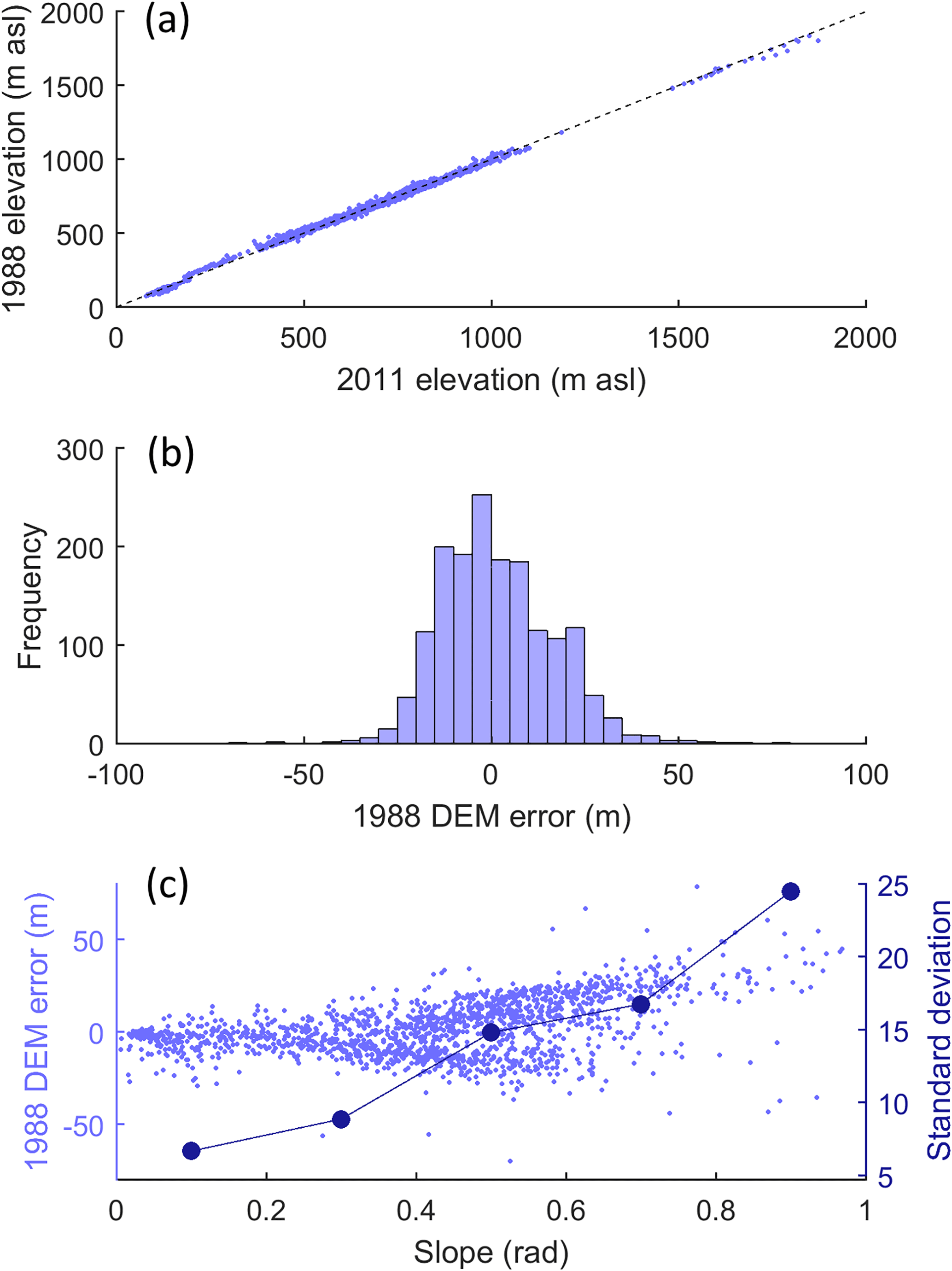
Figure 5 Error model for estimating uncertainty in glacier volume change between 1988 and 2011 including 1988 vs. 2011 off-ice DEM elevations (a), distribution of 1988 DEM errors calculated as the difference between 1988 and 2011 off-ice elevations (b) and estimation of change in standard deviation of errors with the DEM slope (c).

2.5.2 Snow coverage

Having removed the MODIS data that did not pass the QA test including all of the data between September and February, less than 5 % of the remaining data were usable, and therefore, it was decided that these data should be combined to derive three seasonal average snow coverage maps. From these maps, three snow coverage curves were constructed that define the mean catchment snow coverage over an elevation range for three different times of the year: spring (March and April), early summer (May and June) and late summer (July and August) (Fig. 6). The curves provide information on both the spatial and temporal distributions of snowfall in the study catchment. They were constructed by distributing the seasonal average snow distribution maps across the 50 m model grid DEM. For example, for a MODIS pixel value of 0.5, 50 of the corresponding DEM pixels were assumed to be snow covered. The MOD10A1 product cannot distinguish between snow and ice-covered regions, so only data that covered ice-free parts of the catchment were used. This limited the analysis up to a maximum elevation of just under 1200 m a.s.l. While this does not cover the full elevation range of the catchment, Fig. 6 shows that the three curves capture a large amount of variability in seasonal snow cover. From the three snow coverage curves, the mean snow coverage values from the lower, middle and upper terciles of the curves were used as signatures of snow coverage.

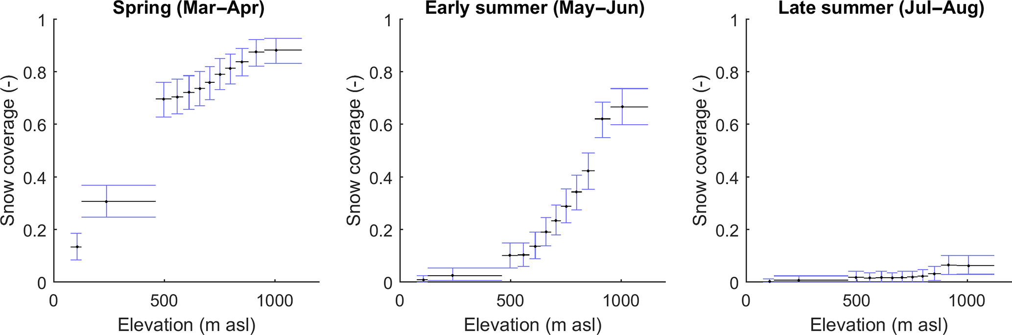
Figure 6 Snow coverage curves defined from the MOD10A1 snow cover product from 2000 to 2015 with 95 % confidence bounds.

There exists no definitive quantification of errors in the MOD10A1 product that can be used to estimate LOA for these signatures. Previous validation of the MODIS data using satellite imagery has shown the data to be relatively robust (Salomonson and Appel, 2004). Accordingly, it was assumed that, as with the ablation stake data, the primary source of uncertainty stems from scale differences between the data and the model simulations. More specifically, because the MODIS data have a coarser resolution (500 m) than the DEM over which the MODIS data were distributed (50 m), a MODIS pixel value of 0.5 only indicates that 50 of the corresponding 100 DEM pixels are snow covered. The construction of a snow distribution curve, therefore necessitates some assumptions about where the snow actually lies which will influence the shape of the snow distribution curve. Accordingly, the LOA were quantified to account for this uncertainty. Here, for each of the seasons, a mean MODIS snow cover map over the study region was derived. Then, for each 500 m pixel, snow was randomly distributed across the corresponding DEM pixels 1000 times. From these, an equal number of snow distribution curves and corresponding snow distribution signatures could be derived, each of which were assumed to be equally probable. The 95 % confidence bounds from this distribution of snow cover signatures were used to define the LOA which are indicated by blue error bars in Fig. 6.

2.5.3 River discharge

The hourly river discharge data for the years 2013 and 2014 measured at ASG1 (Fig. 7a) were used to define 21 different river discharge signatures that cover a range of temporal scales and flow magnitudes. The majority of these signatures were based on previous studies (Schaefli, 2016; Shafii and Tolson, 2015; Yadav et al., 2007; Yilmaz et al., 2008).

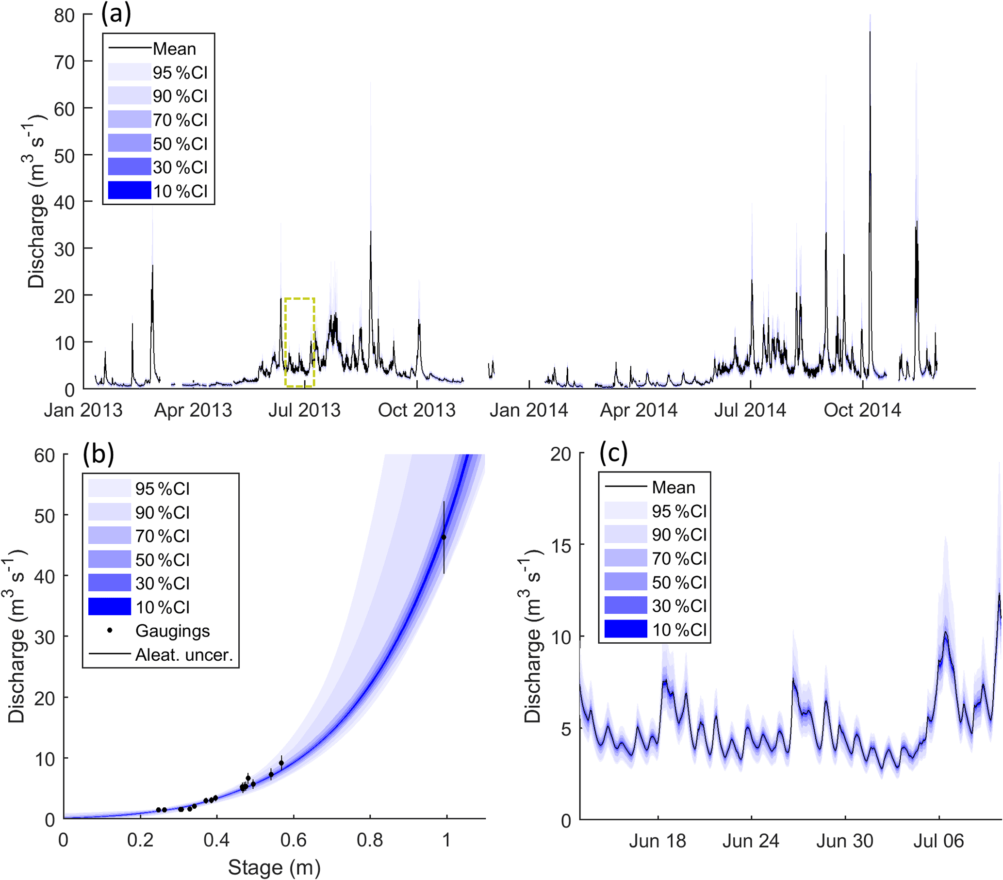
Figure 7 River flow time series from ASG1 with quantified confidence intervals (a), rating curve uncertainty used to quantify confidence intervals (b) and zoomed section of river flow time series (see yellow dashed box in top plot) with confidence intervals (c).

Mean monthly river flows were calculated to characterise the seasonal river flow regime. Signatures were also derived from sections of the flow duration curve to characterise quick-release high flows and slow-release low flows. These include signatures that quantify the volume under the section (flow magnitude) and the slope of section (flow variability) for the low-flow section (99–66 % flow exceedance), high-flow section (15–5 % flow exceedance) and highest-flow section (5–0.5 % flow exceedance). An overall estimate of flow variability, the coefficient of variation, was also calculated. Related to this, two further signatures, the rising limb density and integral scale, provide a measure of flashiness. The rising limb density is the ratio of the number of flow peaks to the total time to peak where a higher number is more flashy. The integral scale measures the lag time at which the autocorrelation function of the flow time series falls below $\frac{\mathrm{1}}{e}$ (diurnal cycles in river flow were removed prior to this using a moving average filter). A higher integral scale therefore indicates a less flashy, slowly responding hydrological system. Finally, the peak summer flow hour of the observed discharge time series was calculated to characterise the intra-day river discharge response to melt.

Estimates of river discharge are inherently uncertain (Pappenberger et al., 2006). McMillan and Westerberg (2015) provide a useful definition of two important sources of uncertainty which they distinguish as either aleatory (random) or epistemic (of an unknown character). The first stems from random measurement errors such as those from the instrument used for periodic river gaugings. These cause gauging points to vary around the “true rating curve”, typically according to some formal statistical definition. Epistemic uncertainty stems from the assumptions hydrologists have to make when constructing rating curves, such as assuming the river bed profile and horizontal flow velocity distribution are relatively stable over time. These errors make fitting a single rating curve to all of the gauging data invalid. Accordingly, McMillan and Westerberg (2015) propose a method to define the rating curve uncertainty which accounts for both sources of error and has been used to estimate uncertainty in river discharge signatures (Westerberg et al., 2016). The random error component was defined from analysis of 27 flow gauging stations in the UK with stable ratings and without obvious epistemic errors (Coxon et al., 2015). They conclude that this source of error is best approximated by a logistical distribution model. To account for the epistemic error, they reject the assumption that the rating curve is fixed in time and instead they fit an ensemble of rating curves to all of the gauging data. Each curve is weighted by a “voting point” likelihood function which scores it based on how many points of the periodic gaugings it is able to intersect (and at what location in the logistical distribution of each measurement).

In this study, the methodology proposed by McMillan and Westerberg (2015) was used to estimate rating curve uncertainty. Markov chain Monte Carlo sampling was used to define 667 unique rating curves which together define the rating curve uncertainty (Fig. 7b). From these an equivalent distribution of each river discharge signature was derived from the ensemble of flow time series (Fig. 7c), from which the 95 % confidence bounds were used as the LOA. Because the voting point method only accounts for uncertainty in the flow magnitude and not the timing, it was not suitable to apply this approach to the three signatures that characterise melt run-off timing and flashiness. For these signatures, Schaefli (2016) proposed that the LOA should be derived by subsampling different periods of the flow time series. For this study a month-by-month subsampling strategy was employed to do this.

2.6 Model calibration procedure

The GHM was configured to run from 1988 to 2015 so that simulations could be compared against all observation signatures. The initial ice surface was set to the 1988 DEM of the ice, while the bedrock and land surface topography were taken from the Öræfajökull bedrock map (Magnússon et al., 2012). Initial snow coverage, soil moisture, linear reservoir storages and ELA were determined by running the model for 3 consecutive years prior to the simulation period using climate data from 1985 to 1988.

In total there were nine possible structural configurations of the GHM including all possible combinations of the three melt and run-off-routing model structures. For each of the nine configurations, the melt and run-off-routing model parameters were calibrated to achieve the closest fit to the observed signatures. To do this, first a set of preliminary runs were undertaken to assess the sensitivity of the simulations to the parameters. Here, it was found that the simulations were insensitive to the firn melt parameters across the range of 33 signatures. Accordingly, these were set to the same values as for snow. Similarly, none of the signatures were sensitive to the threshold above which melt occurs, T^*, and accordingly, this was set to 0 ^∘C throughout the model experiments. Finally, it was also decided to fix the albedo parameter for ice in TIM₃ to 0.3. This was because this parameter directly interacts with the b parameter and therefore provides no extra control over model behaviour.

The remainder of the parameters were kept for calibration (see Table C1). For each GHM configuration, 5000 Monte Carlo simulations with random parameter sets sampled from predefined uniform distributions were undertaken. The prior parameter distributions were defined from a review of previous modelling studies and later refined during the preliminary runs noted above. The quasi-random Sobol sampling strategy (Brately and Fox, 1988) was employed to sample the parameter space as efficiently as possible. The simulated signatures from each model run (parameter set) were then evaluated against the observed signatures using a continuous acceptability score:

$$\begin{array}{}\text{(9)}& s_j=\left\{\begin{array}{ll}\mathrm{0}& {\text{low}}_j\le {\text{sim}}_j\le {\text{upp}}_j\\ \frac{{\text{sim}}_j-{\text{upp}}_j}{{\text{upp}}_j-{\text{obs}}_j}& {\text{sim}}_j>{\text{upp}}_j\\ \frac{{\text{sim}}_j-{\text{low}}_j}{{\text{obs}}_j-{\text{low}}_j}& {\text{sim}}_j<{\text{low}}_j\end{array}\right.,\end{array}$$

where obs_j and sim_j are the observed and simulated values for signature j and upp_j and low_j are the upper and lower LOA. Here, a score of zero indicates that the model captures the observed signature within the LOA. An absolute score greater than 0 is outside of the LOA and therefore unacceptable. The sign of the score indicates the direction of bias, while its magnitude indicates the model's performance relative to the LOA. A score of −3 would indicate that the model underestimates the signature by 3 times the observation uncertainty.

Given that there are 33 different signatures to calibrate to simultaneously, it was important to define a weighting scheme to achieve the best overall performance across the range of signatures. It was decided that, for a given GHM configuration, the 5000 runs should be ranked by a weighted average score where each group, each attribute within each group and each signature within each attribute were given equal weighting so that the scores were not biased to a particular group or attribute. The top 1 % of model runs that achieved the smallest weighted average acceptability scores were then taken as the calibrated models for each GHM configuration and the average acceptability scores of these are reported. A bootstrapping with a replacement resampling scheme was also used to assign 95 % confidence intervals around all reported acceptability scores. While not a formal test of statistical significance, these were used to avoid reporting differences between the GHM configurations where issues such as undersampling of the parameter space would make such conclusions unjustified. Where confidence intervals do not overlap, differences are hereafter referred to as substantial. The different GHM configurations were also compared when calibrated to individual groups of signatures (ice melt, snow coverage and river discharge). In this case the same weighting procedure was applied to a single group only.

3 Results

3.1 Signature discrimination power

As a first step towards evaluating the LOA framework, the discrimination power of the signatures was investigated to determine their relative usefulness for discriminating between acceptable and unacceptable model structures and parameterisations when used individually. A total of 45 000 calibration runs, each with unique model structures and parameterisations (hereafter referred to as model compositions) were undertaken in this study. The signatures with the highest discrimination powers were defined as those that best constrain the range of acceptable model compositions. Here, the total number of acceptable model compositions were calculated for each signature as an indicator of discrimination power (bars in Fig. 8a). The results indicate that the ice melt signatures are the best discriminators. Of these, the winter melt signature from the ablation stake measurements is the best discriminator, while the summer melt signature shows the least discrimination power. The snow coverage signatures generally are shown to be inferior discriminators when compared to the ice melt signatures. The late-summer snow coverage signature for the lower catchment is shown to be the poorest discriminator, presumably because there is negligible snow cover here at this time of the year: an observation that almost all of the model compositions have no difficulty in replicating. In contrast, no model compositions are deemed acceptable for the signatures of the spring and early-summer snow coverage in the upper catchment.

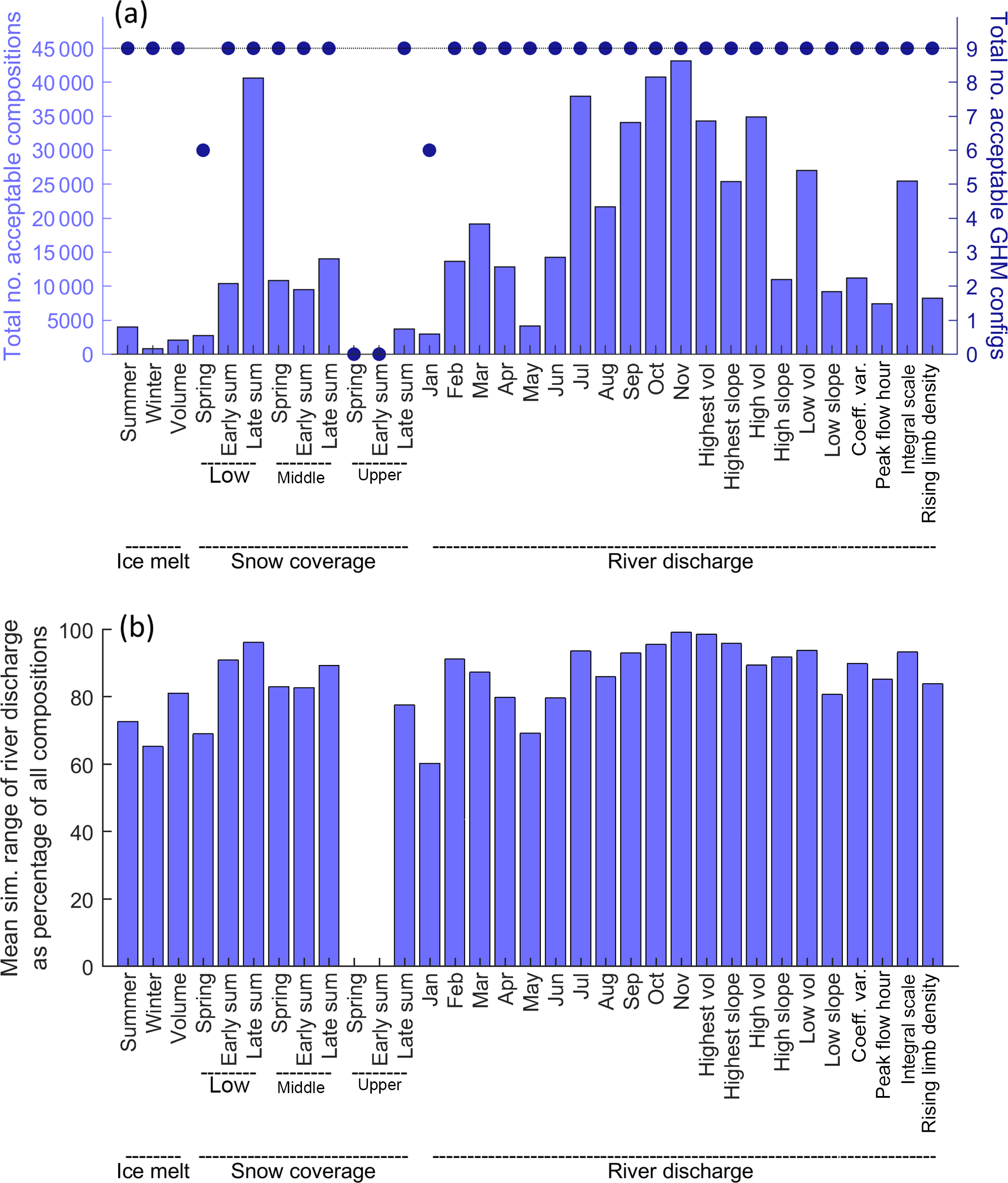
Figure 8 Total number of acceptable model compositions (bars) and configurations (dots) for each signature (a) and mean simulated range in river discharge from the population of acceptable models as a percentage of the simulated range using all of the 45 000 model compositions (b).

The discrimination power of the river discharge signatures is shown to be highly variable, but there are several discernible patterns. Firstly, the mean monthly flow signatures between January and June, when river discharge is low, are shown to be better discriminators than the higher-flow signatures from July to October. The mean monthly January and May flows stand out as being particularly powerful at discriminating between acceptable and unacceptable model compositions, suggesting that these are likely to be focal points for characterising model deficiencies. Those signatures related to the variability of flows such as the coefficient of variation and the flow duration curve slope signatures, as well as peak flow hour (timing) and rising limb density (flashiness) are also shown to be relatively good discriminators.

To determine the structural discrimination power of each signature, the total number of GHM configurations that returned at least one acceptable simulation have also been calculated for each signature (scatter in Fig. 8a). They show that, when used individually, most of the discrimination power stems from constraining the parameter space rather than constraining the structural space. Only the lower-catchment spring snow coverage and mean January river flow signatures discriminate between structures where only six of the nine GHM configurations returned acceptable simulations. In both cases it was the GHM configurations that employed the TIM₃ melt model structure that could not capture these signatures within their LOA.

To indicate how each signature helps to reduce river flow prediction uncertainty, a second measure of discrimination power has also been calculated (Fig. 8b). Here, the mean simulated range in river discharge from the population of acceptable models has been calculated as a percentage of the simulated range using all of the 45 000 model compositions for each signature. These results show that when used individually, all of the signatures help to constrain the river flow prediction uncertainty, although the effectiveness of each is variable. The mean January and May river flow signatures again exhibit good discrimination power, reducing the mean river discharge uncertainty to 60–70 % of that from the full population of model compositions. Similarly, the winter ice melt and spring snow coverage in the lower catchment remain two of the best discriminators. However, some signatures, such as the long-term volumetric change in the glacier, which was a good discriminator of model acceptability, are not as effective at reducing river discharge prediction uncertainty.

3.2 Acceptability of melt model structures

While all signatures clearly demonstrate discrimination power when used individually, it remains to be seen how effective the LOA framework is for discriminating between and diagnosing deficiencies in different model structures when using multiple evaluation criteria. Here, the acceptability scores obtained after calibrating the GHM to the different groups of signatures (ice melt, snow coverage and river discharge) using the three different melt model structures have been calculated (Fig. 9). The light-grey boxes indicate those signatures that have been captured within the LOA, and the dark-grey boxes and their corresponding acceptability scores indicate those signatures which the structures were not able to capture within the LOA. So that the river discharge acceptability scores can be compared fairly, they have all been obtained using the ROR₁ run-off-routing structure.

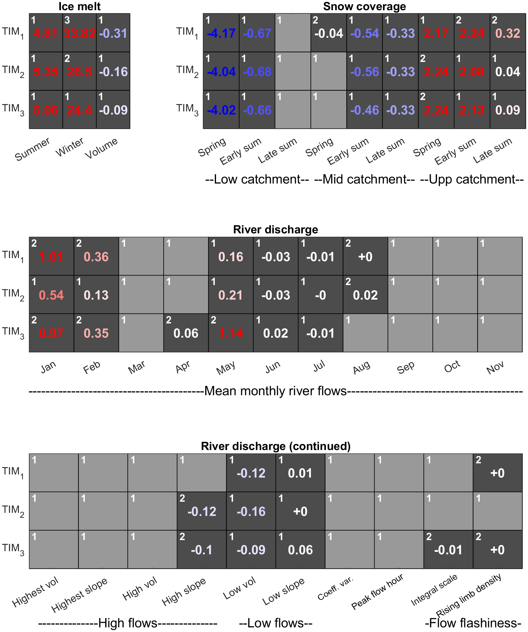
Figure 9 Acceptability scores obtained after calibrating the GHM using the three melt model structures in combination with the ROR₁ run-off-routing model structure. The three GHM configurations were calibrated against ice melt, snow coverage and river discharge signatures separately. Light-grey boxes indicate acceptable simulations (s=0) and numbered, dark-grey boxes indicate unacceptable simulations coloured blue and red to indicate negative and positive biases respectively. Note that all acceptability scores are rounded to two decimal places. Those non-zero scores that round to zero are accompanied by ± to indicate sign of score. White numbers in the top left of each box indicate relative ranking where acceptability scores are substantially different between the GHM configurations.

When calibrated against the ice melt signatures, the GHM is not able to capture them within their LOA, regardless of the melt model structure used. The different GHM configurations show a tendency to overestimate the measured summer and winter melt from the ablation stake data, yet underestimate the long-term change in total ice volume (note underestimation here refers to the simulated loss in ice volume). This highlights a deficiency in the melt model structures as they are unable to reconcile the three melt signatures simultaneously within the observation uncertainty. The winter melt is by far the most unacceptable simulation, particularly when using the TIM₁ structure, which overestimates it by more than 30 times the observation uncertainty.

Each of the GHM configurations using the three melt model structures have been ranked from 1 to 3 in the top left corner of each box where the acceptability scores are substantially different (Fig. 9). While there are clearly differences in the acceptability scores for the summer melt and ice volume signatures, they are not substantially different and therefore it is not possible to say that one structure is more acceptable than another. Indeed, a comparison of the simulated ice thickness change along the Falljökull and Virkisjökull arms of the glacier reveal that all three configurations of the GHM produce almost identical simulations which broadly capture the observed ice thickness change between 1988 and 2011 (Fig. 10).

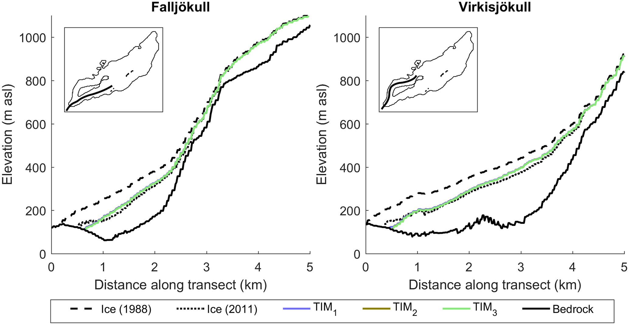
Figure 10 Observed and simulated ice thickness change as measured along the transects of the Falljökull and Virkisjökull glacier arms. Insets show transect locations.

For the winter melt signature, there is a substantial difference in acceptability when using the three melt model structures. Here, the GHM configuration using the TIM₃ structure is the most acceptable, while using the TIM₁ structure is least acceptable, indicating that, while all configurations produce simulations outside of the LOA, there is an improvement in ice melt simulations when implementing the most sophisticated TIM₃ melt model structure.

For the snow coverage signatures, all three of the GHM configurations capture the late-summer snow coverage in the lower portion of the catchment within the LOA. When using the TIM₂ and TIM₃ structures, the mid-catchment spring snow coverage is also captured. The remaining snow coverage signatures are not captured within the LOA, where all configurations show a tendency to underestimate snow coverage in the lower and middle parts of the catchment and overestimate snow coverage in the upper part of the catchment. To investigate why this is, Fig. 11a shows the simulated early-summer mid-catchment and upper-catchment snow coverage signatures for the 5000 calibration parameter sets (blue dots) used with the TIM₁–ROR₁ GHM configuration. Here it can be seen that, regardless of the choice of melt model parameters, this structure is not able to capture both of these signatures within their LOA simultaneously (indicated by yellow area). A similar inconsistency exists when comparing snow coverage over different seasons where the GHM is not able to capture the lower-catchment snow coverage in the early summer and spring simultaneously (Fig. 11b). Indeed, this inconsistency extends across all melt model structures.

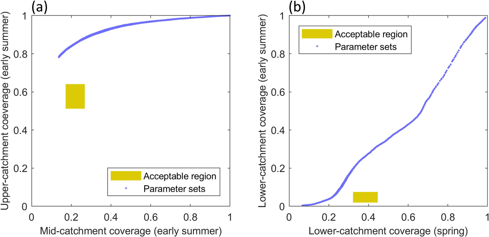
Figure 11 Simulated snow coverage signatures from the 5000 calibration runs (blue dots) for the TIM₁-ROR₁ GHM configuration including early-summer mid-catchment and upper-catchment snow coverage signatures (a), and lower-catchment spring and early-summer snow coverage signatures (b).

A comparison of simulated snow distribution curves from the calibrated models (Fig. 12) reveals that all return similar simulations. The simulation using TIM₁ deviates slightly from the curve produced by the GHM when using the TIM₂ and TIM₃ structures, but overall the choice of melt model structure has a limited influence on the simulated seasonal snow coverage.

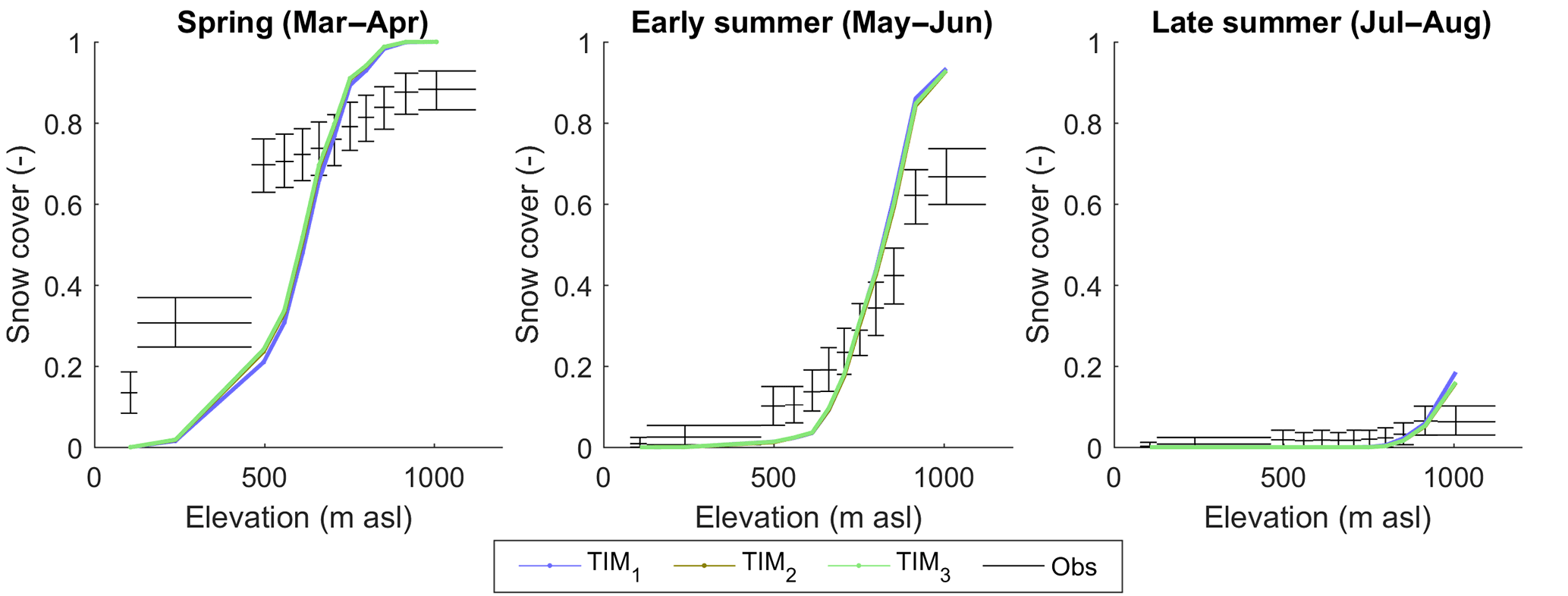
Figure 12 Simulated seasonal snow distribution curves when using the three melt model structure.

The acceptability scores for the river discharge signatures in Fig. 9 show that, regardless of the choice of melt model structure, when used in conjunction with the ROR₁ run-off-routing model structure, all are able to capture a range of river discharge signatures. The simplest GHM configurations using the TIM₁ and TIM₂ model structures capture 12 river discharge signatures simultaneously within the LOA, while the inclusion of the dynamic snow albedo term and re-arrangement of the melt equation in the TIM₃ melt model actually inhibits the GHM performance where only 10 of the 21 river discharge signatures are captured within the LOA.

The mean monthly flow signatures for January, February and May show some of the highest absolute acceptability scores, indicating the models are least efficient at capturing these. For winter flows in January and February, the simulation using the TIM₂ model structure is substantially more acceptable than when using the other melt model structures, although it should be noted that, given that flows are very low here, the absolute error is less than 0.2 m³ s⁻¹. A comparison of the simulated ice melt during May 2013 reveals that the TIM₃ structure simulates the highest ice melt of all three melt model structures (Fig. 13a), which results in a positively biased river flow time series (see Fig. 13b). Note that the full input/output time series over the observation period can be found in Appendix D.

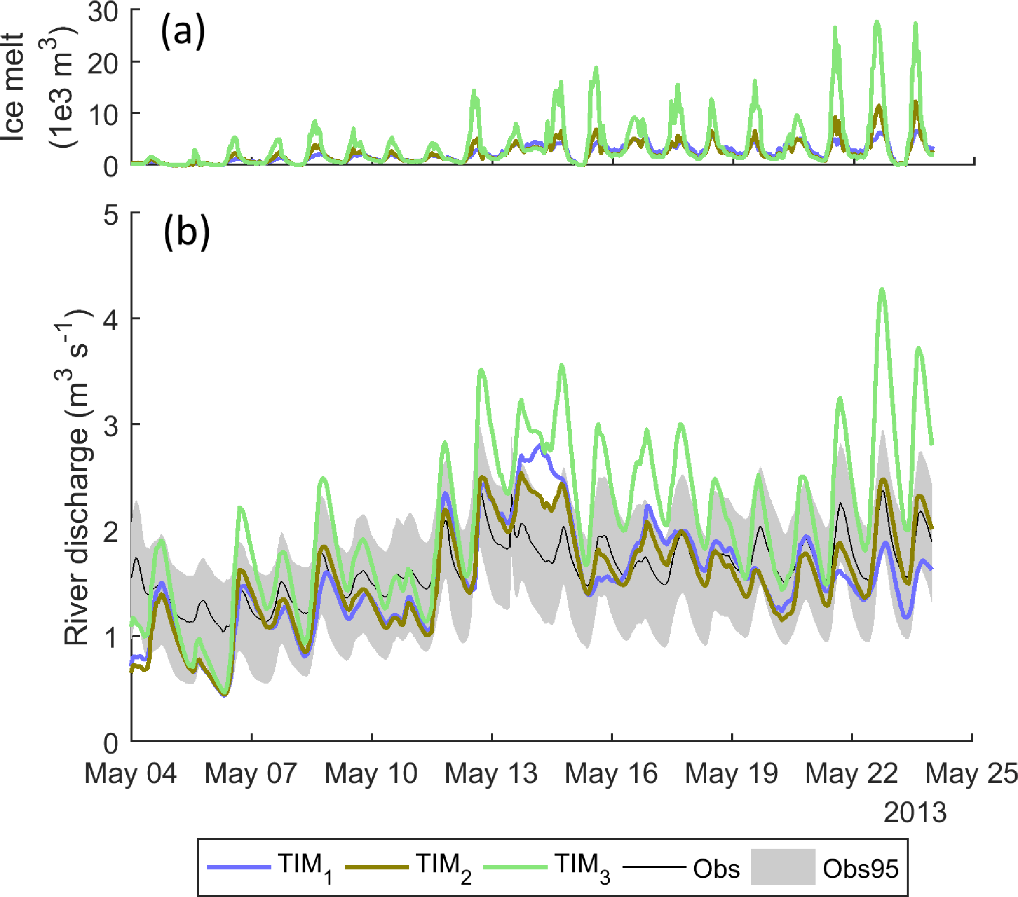
Figure 13 Mean simulated hourly ice melt (a) and river discharge (b) during May 2013 using the top 1 % of models from the three melt model structures in combination with the ROR₁ run-off-routing model structure.

Furthermore, a comparison of the simulated ice melt time series over 2013 with a monthly moving-average filter demonstrates that the positive melt bias from TIM₃ extends between April and June (Fig. 14b), which corresponds to the period in which temperatures are relatively low but incoming solar radiation is relatively high (see Fig. 14a).

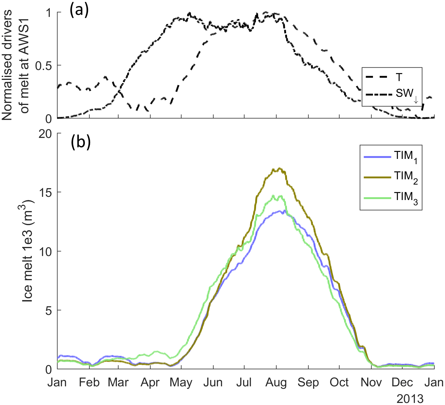
Figure 14 Normalised temperature and incident solar radiation (a) and simulated ice melt from the three calibrated ice melt model structures (b) for the year 2013. All time series use a monthly moving average filter.

Of the remaining river discharge signatures, only a handful show any substantial difference when switching between the melt model structures including the mean April and August discharge and the two flashiness signatures: the integral scale and the rising limb density. However, the differences here are very small. For the high-slope signature, which characterises the variability of high-flow river flows, the simulation using the TIM₁ melt model structure is able to capture it within the LOA, while the simulations using the TIM₂ and TIM₃ model structures both show a negative bias, suggesting they underestimate high-flow variability.

3.3 Acceptability of run-off-routing model structures

To evaluate the run-off-routing model structures, acceptability scores have been calculated for the river discharge signatures only, as these structures do not influence ice melt or snow coverage (Fig. 15). To ensure a fair comparison between the different structures, all scores have been obtained using the simplest TIM₁ melt model structure in the GHM.

It was noted previously that all melt model structures used in combination with ROR₁ resulted in positively biased January and February river flows. It could be that including a more complex non-linear run-off-routing model structure in the GHM could help to mitigate this bias. Indeed, the calibrated simulations do show a substantial reduction in positive bias for the mean February flows when using ROR₂ and ROR₃; however the simulations are still unacceptable. Furthermore, for the mean January river flow there is no substantial change in acceptability score.

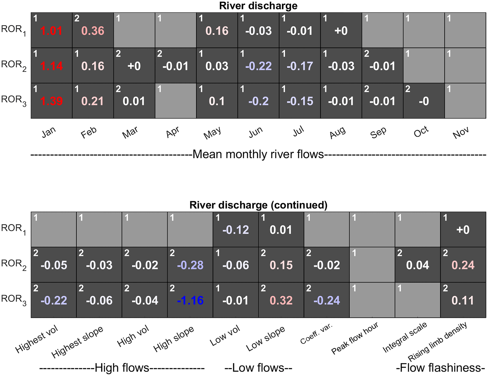
Figure 15 Acceptability scores obtained after calibrating the GHM using the three run-off-routing model structures in combination with the TIM₁ melt model structure. Light-grey boxes indicate acceptable simulations (s=0) and numbered dark-grey boxes indicate unacceptable simulations, coloured blue and red to indicate negative and positive biases respectively. Note that all acceptability scores are rounded to two decimal places. Those non-zero scores that round to zero are accompanied by ± to indicate sign of score. White numbers in top left of each box indicate relative ranking where acceptability scores are substantially different between the GHM configurations.

This indicates that the run-off-routing representation is also not the reason for the overestimation of flows at the beginning of the year. To investigate this positive bias further, Fig. 16c shows the simulated time series from the calibrated models using TIM₁ in combination with ROR₁, ROR₂ and ROR₃ for January and February 2013. Figure 16a shows that input from melt is insignificant during these winter months (green line). Rather it is rainfall (black dash) that dominates the run-off input and this results in two pronounced peaks in the simulated river discharge time series. The different behaviour of the simulations using the three run-off-routing model structures is much more obvious during the rainfall-run-off events. The simulation using the ROR₁ structure is noticeably more flashy in response to the rainfall and overestimates the peak flows, while the ROR₂ and ROR₃ simulations, which include additional, more diffusive representations of the flow of water through snow and firn, result in peak flows that are closer to the observations, but with a recession that is too shallow. Regardless of these deficiencies, however, all result in an almost identical positive bias as shown by the cumulative flow in Fig. 16b.

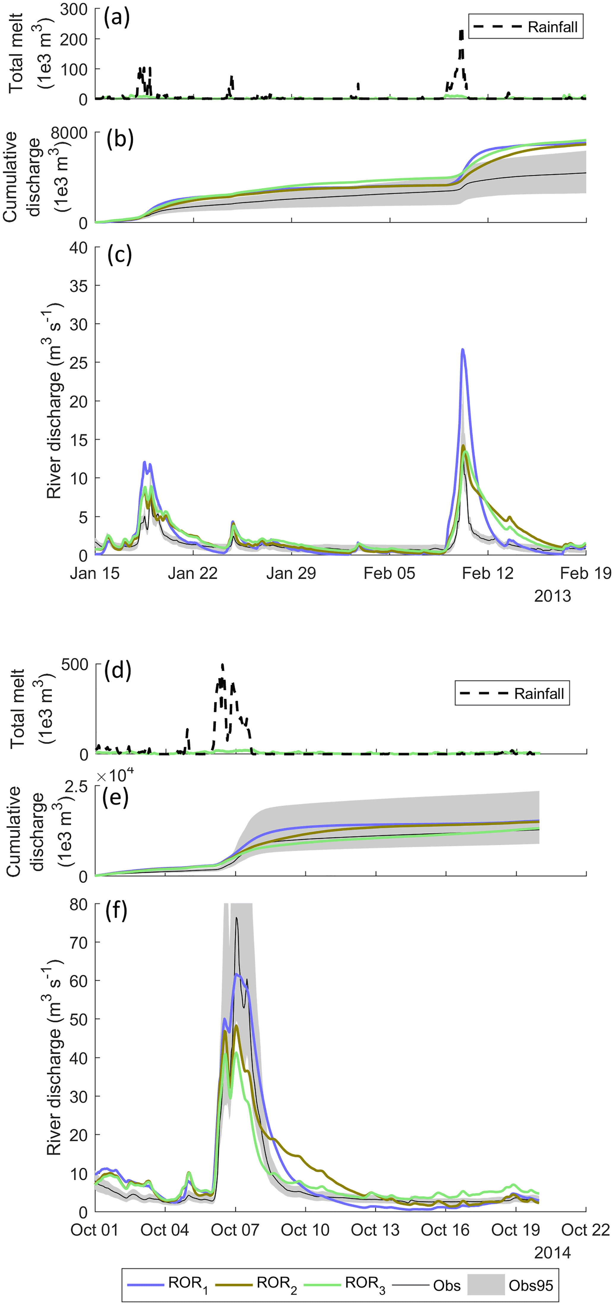
Figure 16 Simulation time series using the three different run-off-routing model structures in combination with the TIM₁ melt model structure including simulated total melt and rainfall (a), cumulative river discharge (middle) and river discharge time series (bottom) for January and February 2013 (a, b, c) and the October 2014 flood (d, e, f).

There are, however, differences when assessing other aspects of the river discharge time series, particularly in the signatures relating to high flows. In Fig. 15, it can be seen that, while the simulation using the ROR₁-routing model structure is able to capture all of the high-flow signatures simultaneously, the ROR₂ and ROR₃ structures show an unacceptable negative bias for these signatures, indicating underestimation of high-flow magnitude and variability. To evaluate this in more detail, Fig. 16f shows the simulated time series for the highest recorded river flow event during October 2014. Here, the flashier and more responsive ROR₁ structure achieves the closest fit to the observed peak flow and within the uncertainty bounds, while the more diffusive, ROR₂ and ROR₃ structures underestimate the peak flow. Note they also underestimate the overall river flow variability as indicated by the coefficient of variation signature.

3.4 Consistency of melt model structures

The results so far have highlighted some inconsistencies in the GHM configurations using the melt and run-off-routing model structures, which are unable to reconcile some combinations of signatures simultaneously. This is important as those inconsistencies could help to further diagnose structural deficiencies in the different model structures. To investigate this, consistency scores have been calculated between pairs of the 33 signatures for each GHM configuration. A model can be deemed consistent across a pair of signatures if it is able to capture them within their LOA simultaneously. The consistency scores are therefore calculated as the minimum sum of the two acceptability scores between a pair of signatures across the 5000 calibration runs for each GHM configuration.

Figure 17 shows the average consistency scores calculated across the signatures for each attribute of ice melt, snow coverage and river discharge using the three melt model structures in combination with the ROR₁ run-off-routing structure. The top panel shows the consistency scores when using the simplest TIM₁ melt model structure. The regions in red highlight the areas where the GHM is inconsistent. The first striking observation is the red band along the upper-catchment snow coverage attribute. It has already been demonstrated that the simulations using the TIM₁ structure cannot reconcile the upper-catchment snow coverage with the remaining snow coverage signatures. This further demonstrates that, when using the TIM₁ structure, the GHM cannot reconcile the upper-catchment snow coverage with any of the other attributes.

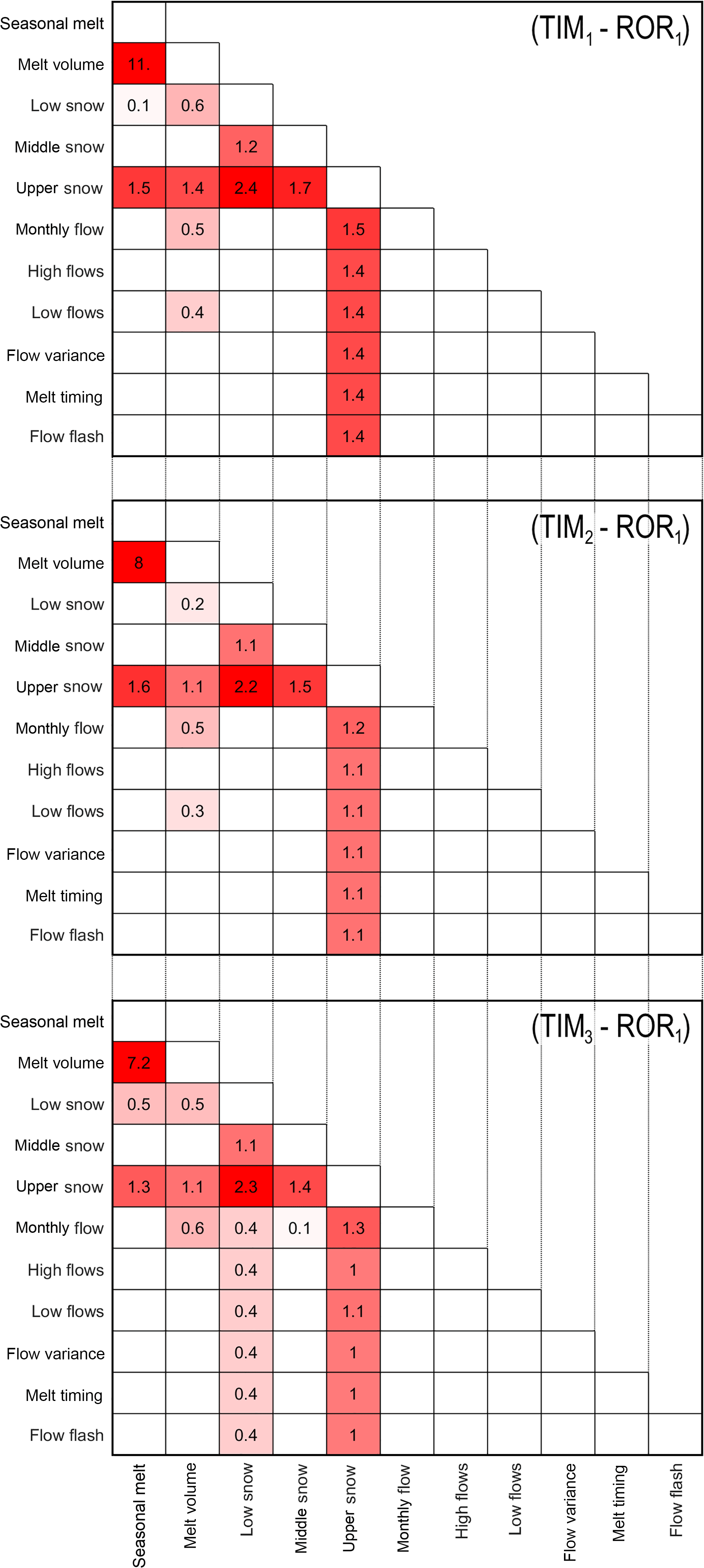
Figure 17 Average consistency scores between attributes using the three melt model structures in combination with the ROR₁ run-off-routing structure. Scores of < 0.1 have not been reported.

The largest inconsistency score obtained was between the short-term, seasonal melt on the glacier tongue and long-term total glacier volume change. It should be noted that the seasonal melt signatures show a small inconsistency with the lower-catchment snow coverage and a larger inconsistency with the upper-catchment snow coverage. The total glacier volume change signature, however, is also inconsistent with the monthly flow and low-flow signatures, indicating that it is the long-term glacier wide mass balance that the model is getting wrong.

The use of the TIM₂ model structure, which includes topographic effects, goes some way to reducing most of the inconsistencies shown using the TIM₁ model structure (Fig. 17). However, all but one of the inconsistencies (between lower-catchment snow coverage and seasonal melt) remain, indicating that the use of the TIM₂ melt model structure only provides a small improvement in model consistency.

Using the TIM₃ model structure also helps to improve model consistency, particularly for the upper snow coverage signatures, but surprisingly it also introduces new inconsistencies in relation to the lower-catchment snow coverage, where the model is not able to reconcile these signatures with any of the other attributes.

3.5 Consistency of run-off-routing model structures

Consistency scores have also been calculated for each pair of river discharge signatures (Fig. 18) using the three run-off-routing structures in combination with the TIM₁ melt model structure. The simulations using the ROR₁ structure (top panel) and next simplest ROR₂ structure (middle panel) show very similar patterns of model inconsistency. Firstly, both sets of simulations do not capture the relatively low flows in February and the relatively high flows in July and August simultaneously. This corroborates the findings from the acceptability analysis which revealed a tendency for the model structures to overestimate low flows in the winter and underestimate high flows in the summer and autumn, particularly with relation to rainfall-induced high flows. Interestingly though, the seasonal flow inconsistency is centred on February and there are not inconsistencies for the other low-flow months from January to April. This provides further evidence that it is particularly the rainfall-induced flows that the model is not able to capture effectively. In fact, February has some of the highest flows in the record of winter flows induced by large rainfall events (see average flow signatures in Table 2). This suggests that this could be the reason that the inconsistencies between winter and summer flows are centred around these months. The inclusion of additional flow pathways in the routing routine only enhances these inconsistencies, particularly when using the ROR₃ model structure where the inconsistencies extend into June (bottom panel).

The ROR₁ simulations show inconsistencies between the February flows and low-flow variability as indicated by the low-slope signature. The reason for this is not clear, but interestingly, the inclusion of an extra, more diffuse, flow pathway in the ROR₂ model appears to remedy this, suggesting that there is some non-linear behaviour that the ROR₁ model structure cannot capture. However, it comes at the cost of inducing an extra inconsistency between the mean flows in January and the overall flow variability as indicated by the coefficient of variation. This new inconsistency is amplified when using the ROR₃ structure.

Interestingly, the consistency scores when using the ROR₁ and ROR₂ structures are relatively similar, with each configuration demonstrating inconsistencies between four and five pairs of river discharge signatures. In contrast, using the most complex ROR₃ structure introduces a number of new inconsistencies with a total of 12 inconsistent pairs of simulated river discharge signatures. These new inconsistencies are centred around the mean monthly flow signatures as well as the signatures relating to high- and low-flow magnitude and variability.

Figure 18 Average consistency scores between river discharge signatures using the three run-off-routing model structures in combination with the TIM₁ melt model structure.

4 Discussion

The first aim of this study was to investigate whether a signature-based approach within a LOA framework could be used to diagnose deficiencies in the different melt and run-off-routing model structures. The comprehensive set of signatures provided a powerful method with which to evaluate the model behaviour. Furthermore, when used within a LOA framework, it was straightforward to identify those aspects of the glacio-hydrological system that the GHM configurations could not capture. A number of the identified model deficiencies are particularly important in the context of future river flow predictions, which will now be discussed.

Regardless of the choice of melt model structure, all GHM configurations were able to capture the three signatures of ice melt individually, but none of them could capture all of the signatures simultaneously. The challenge here was to reconcile three signatures that characterise glacier melt over different spatial and temporal scales. This is not a straightforward task, particularly when using temperature index models that lump a number of spatially and temporally variable terms from the full energy balance equation into a handful of calibration parameters which may lack robustness in space and time (Gabbi et al., 2014; MacDougall et al., 2011; Matthews et al., 2015). The inclusion of solar and topographic effects in the TIM₂ and TIM₃ melt model structures addressed some of these limitations. Indeed, their inclusion in conjunction with the dynamic snow albedo parameterisation returned the most acceptable simulations of the ice melt signatures overall. However, further improvements are required to achieve acceptable model simulations that capture all of the ice melt signatures simultaneously. Certainly, one aspect of the glacier which was not accounted for was debris cover at the glacier terminus, which could be an important control for point scale and overall ice mass balance. Some TIMs that include representations of debris cover do exist (Carenzo et al., 2016) and the signature-based LOA approach would provide the ideal framework for evaluating the added value of further structural modifications like these.

The snow coverage signatures highlighted deficiencies in all of the GHM configurations. None of the prior 45 000 model compositions were able to capture the spring and early-summer snow coverage in the upper catchment and all of the calibrated GHM configurations overestimated snow coverage in the upper catchment while underestimating it in the lower catchment. Interestingly, using the most sophisticated TIM₃ structure with the dynamic snow albedo function had almost no effect on the overall acceptability across these signatures, indicating that the melt model formulation was not the primary source of model deficiencies here. Of course, snow coverage simulations are sensitive to other components of the GHM, such as the snow redistribution model, which itself is sensitive to the resolution of the DEM used to parameterise it; a coarser DEM resolution removes peaks and troughs in the land surface which can bring about more complex patterns of snow coverage. Similarly, the glacier volume change signature will be sensitive to the glacier evolution formulation and parameterisation. It is clear, therefore, that, while the application of a LOA framework here has demonstrated the gains that can be made in capturing some signatures through the inclusion of extra model complexity, the apparent insensitivity of the snow coverage signatures to structural modifications indicates that further gains may also be made by investigating other components of the GHM structure within this framework. Beyond the structural nature of a GHM, the boundary conditions may also contribute to model deficiencies. For this study, the driving precipitation data were relatively well constrained by observations within the catchment during the summer and autumn months of recent years, but there were fewer observations during the winter months and none at all before 2009. Furthermore, while the bias-corrected precipitation time series was well correlated over a 3-day time step, it was not at an hourly time step. It is also important to note that precipitation observations were all collected at the bottom of the catchment and therefore driving precipitation data at the top of the catchment are less certain. Indeed, one could explain the tendency to overestimate snow coverage higher up in the catchment by a positive bias in the driving precipitation data here. Such a bias could also explain the modelled inconsistencies across signatures that characterise ice melt at different spatio-temporal scales. Furthermore, given the strong coupling between snow, ice and river run-off, deficiencies in capturing the snow and ice signatures could also propagate through the hydrological representation of the catchment. For example, one could imagine how errors in the spatial distribution of snow could perturb the timing of run-off through the catchment given that snow distribution influences the behaviour of the semi-distributed run-off-routing routine employed in the GHM. Such perturbations are likely to impact the ability of the GHM to capture the full range of river discharge signatures. Accordingly, it is important to stress the influence that biases in the driving climate data could have on the model acceptability across the different signatures. Of course, for balance, it should be noted that regarding precipitation higher up in the catchment, the limited precipitation collected at the summit of Öræfajökull indicate that mean annual biases in driving precipitation data are small (Guðmundsson, 2000). Even so, the recent melt model comparison by Reveillet et al. (2017) suggest that uncertainties in driving precipitation data can cloud any differences in melt model behaviour.

As a side experiment, we tried increasing the snowmelt parameters for the TIM₃ model to see whether this would help remove some of the inconsistencies across the ice and snow signatures. It was found that using snowmelt parameters equal to or even greater than those used for the ice reduced (improved) the consistency score between the ice melt signatures by more than 50 % when using TIM₃. The physical justification of this is of course questionable, but it does highlight the influence that the prior parameter distributions could have on the results presented here. Accordingly, different specifications of the calibration parameter ranges may also help to improve model consistency.

The main deficiencies noted for all of the GHM configurations when compared to the river discharge signatures were an overestimation of the relatively low winter flows in January and February, and the flows at the start of the melt season in May. It was assumed that the additional slow flow pathways in the ROR₂ and ROR₃ run-off-routing structures would help to correct for any deficiencies in capturing the hydrograph seasonality. Instead, the choice of run-off-routing structure had very little influence on these signatures, indicating that longer-term storages of water do not significantly control the seasonality of the hydrograph. This is probably because of the catchment's small size, which leads to an instantaneous seasonal response to melt on a monthly timescale. We suggest, however, that for larger catchments, the monthly flow signatures are likely to be more sensitive to the choice of run-off-routing structure. Instead, the simulated mean monthly river flow signatures were more sensitive to the choice of melt model structure, particularly in May at the start of the melt season, which is not surprising given the high degree of glaciation of the river basin. Even so, regardless of the melt model structure employed, none of the GHM configurations could correct for the biases in mean monthly flows, indicating that further structural modifications are required. One process that is not represented at all in any of the GHM configurations, but which has been shown to be important in for Icelandic glaciers, is refreezing of meltwater and rainfall (Johannesson et al., 1995). It is estimated that about 7 % of total melt in valley glaciers in Iceland refreezes, and therefore, the inclusion of this process could also help to reduce run-off during the colder months of January and February.

In contrast to the monthly river flow signatures, the choice of run-off-routing structure had by far the dominant influence on those signatures that are controlled by flows operating on much shorter timescales such as the distribution of flows, flow variability and flashiness. This hierarchy of influence between the melt and run-off-routing model structures has important implications for river discharge prediction uncertainty in glaciated basins. For example, if one were interested in future seasonal water resource availability, they would be most reliant on predictions of mean monthly river flows. The results here indicate that, for this catchment at least, uncertainties in these predictions stem primarily from melt model uncertainty. In contrast, if one were interested in future changes in flood frequency, the dominant source of model prediction uncertainty is the run-off-routing approach. Uncertainties in river flow predictions from glacio-hydrological models are therefore dependent on the river flow characteristic of interest.

The results from the simulated river discharge signatures also raised some questions about the added value from introducing extra complexity to conceptual models of glacio-hydrological processes. The most sophisticated TIM₃ melt structure was the most consistent across the ice melt and snow coverage signatures. However, it was also the least acceptable structure for the mean May river flow signature, which showed the highest positive bias. This is interesting, as May coincides with the beginning of the main melt season and therefore this could be some indication of an inability to capture this initialisation properly. It was shown that the simulated snow coverage signatures were almost identical when using the three melt model structures, indicating that this deficiency did not stem from the dynamic snow albedo component of TIM₃. Furthermore, May corresponds to the period in which temperatures are relatively low but incoming solar radiation is relatively high, indicating that it is the additive form of the TIM₃ melt equation and the subsequent increased influence of solar radiation on melt which induced the positive bias in flow simulations in the early melt season.

Similarly, the ROR₃ structure, originally proposed as the most realistic conceptual representation of water storage and transmission in the river basin, was the least acceptable model overall across the river discharge signatures. Certainly, the more diffusive behaviour of the ROR₃ run-off-routing structure was advantageous for capturing peak flows during the winter. However, it also resulted in an underestimation of peak flows at the end of the melt season and an underestimation of overall river flow variability. These results highlight the need to exercise caution before introducing complexity to conceptual models of glacio-hydrological processes. They also illustrate the importance of testing prior assumptions about the system against other possible model hypotheses, for which a signature-based LOA framework is ideally suited.

The second aim of this study was to determine whether the signature-based evaluation within a LOA framework could be used to constrain the prior population of model structures and parameter sets (compositions) to a smaller population of acceptable models. The initial discrimination tests showed that all of the signatures have discrimination power, although for two of the snow signatures, none of the 45 000 model compositions could capture them. The mean January and May river flow signatures were the best discriminators, individually reducing mean river discharge uncertainty to 60–70 % of that from the full population of model compositions, although it should be noted that the majority of this reduction stemmed from constraining the acceptable parameter sets rather than the model structures. These results indicate that a LOA framework could be used to find a population of acceptable model compositions. However, the fact that none of the prior 45 000 compositions were able to capture all of the signatures means that this remains to be seen. At a fundamental level, the results indicate that the structural configurations of the GHM employed in this study are simply not good enough to capture the observation data within their observation uncertainty bounds. To address this, one could implement further structural modifications, some of which have been alluded to, until acceptable simulations are obtained. Indeed, a more thorough exploration of a wider parameter space could also yield acceptable model compositions. There are, of course, other sources of unacceptable behaviour. Of these, boundary conditions including the ice and watershed boundaries, as well as the driving climate data, are all contenders. The initial ice geometry was also uncertain but not explicitly accounted for. It is therefore recommended that, where possible, future applications of a LOA framework should incorporate these additional sources of uncertainty, so that more robust conclusions about model appropriateness can be made. Certainly, it is important to emphasise that these future applications need not adopt the same 33 signatures used in this study. On the contrary, the choice of signatures will always depend somewhat on the availability of data at a given study site as well as the complexity (e.g. spatio-temporal resolution) of the model(s) being interrogated. Indeed, future users should be encouraged to experiment with different signatures (where data permits), particularly if they wish to focus on other process representations within their GHM. Study sites with good observation data and an understanding of data uncertainty would be ideal candidates for these future applications.

5 Conclusions

The signature-based, LOA framework adopted in this study provided a comprehensive evaluation of different GHM melt and run-off-routing model structures. In contrast to traditional model evaluation approaches, which rely on one or several global summary statistics, the adoption of multiple signatures helped to identify those aspects of the glacio-hydrological system that a particular model could or could not capture and the added value of introducing additional complexities to simplified process models. When evaluated against individual signatures, the more complex model formulations did improve model simulations in some cases. However, they were not necessarily more consistent across the full range of signatures, emphasising the need to exercise caution and properly evaluate whether additional complexities are justified. The often conflicting acceptability scores across the signatures highlights the difficulty and inherent uncertainty in model structure selection. It is clear, therefore, that future glaciological and hydrological projection studies that use simplified model structures should take into account these uncertainties, although to date they have rarely been considered. For future river flow predictions in glaciated basins it is likely that the source of model uncertainty depends on the particular river flow characteristic of interest. We found evidence that a hierarchy of influence exists between the melt and run-off-routing model structures across the range of river discharge signatures.

An additional advantage of adopting a LOA framework is that it provides objective criterion for accepting or rejecting particular model structures and parameterisations. While all but two of the signatures demonstrated discrimination power, none of the 45 000 different model compositions tested in this study were able to capture them within their LOA simultaneously. Therefore, it remains to be seen if the framework can be used in this way, although we suggest that applications that go beyond examining the melt and run-off-routing structural uncertainties may prove more fruitful in obtaining a behavioural population of models. These should consider other uncertainties including those associated with snow redistribution, glacier evolution and model boundary conditions. We would therefore encourage future studies, particularly with a broad range of observation data covering different aspects of the glacio-hydrological system, to move away from using traditional global summary statistics for model evaluation and adopt a multi-metric approach within a LOA framework so that their simplified process hypotheses can be rigorously tested and their structural uncertainty better understood.

Appendix A: Glacio-hydrological model

A1 Soil infiltration and evapotranspiration

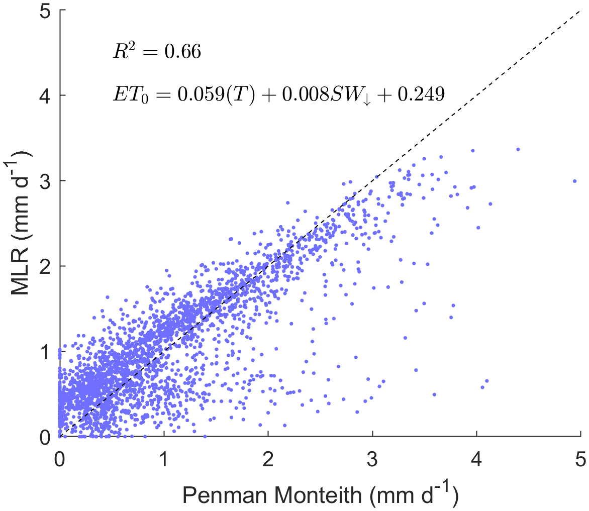
Figure A1 Multiple linear regression model used to convert ambient air temperature and incoming solar radiation into potential evapotranspiration.

The semi-vegetated nature of the catchment coupled with relatively cool temperatures year-round mean that evapotranspiration is generally low (Einarsson, 1972). Even so, to satisfy the water balance, an explicit representation of the soil zone for model nodes that are not ice or snow-covered was included using the method developed by Griffiths et al. (2006), which has been successfully applied to temperate regions in the past (Mackay et al., 2014; Sorensen et al., 2014) and is based on the well-established UN Food and Agricultural Organisation soil water balance method (Allen et al., 1998). For each bare ground node, the soil is represented as a finite storage reservoir with a soil water capacity, termed the total available water, TAW [L], which defines the maximum volume of water available to plants for evapotranspiration after the soil has drained to its field capacity, and can be defined from look-up tables with basic information on vegetation and soil type (Allen et al., 1998). This was parametrised using the Talus soil class and semi-vegetated land surface class, giving an average TAW value of 7 mm. Soil storage is replenished by infiltration from rainfall and melting of residual snow overlying the bare ground and is depleted by evapotranspiration giving a soil water balance:

$$\begin{array}{}\text{(A1)}& {\displaystyle \frac{\mathrm{\Delta }{S}_{\mathrm{soil}}}{\mathrm{\Delta }t}}=I-\mathrm{ET},\end{array}$$

where S_soil [L] is the soil water storage, t is time, I [LT⁻¹] is the infiltration rate and ET [LT⁻¹] is the evapotranspiration rate. Because measured ET is rarely available, Griffiths et al. (2006) propose using the potential evapotranspiration rate, ET₀, instead, which defines the evapotranspiration rate from a reference grass-covered wet soil (see Appendix A2 for calculation of ET₀). Using ET₀ as the maximum possible evapotranspiration rate, they define a separate function which accounts for the fact that as the soil becomes drier, plants find it more difficult to extract moisture from the soil matrix, and therefore ET is typically less than ET₀. While this is conceptually sound, it was decided to not include this function and instead assume that ET = ET₀. There are three reasons for doing this. Firstly, because the inclusion of this function requires an additional parameter which is uncertain and must be calibrated. Secondly, because ET is a relatively small component of the overall water balance in this catchment and it was not the aim of this study to investigate this aspect of the catchment hydrology. Thirdly, because previous studies have shown that this parameter (and therefore the behaviour of this function) is relatively insensitive and unidentifiable (Mackay et al., 2014).

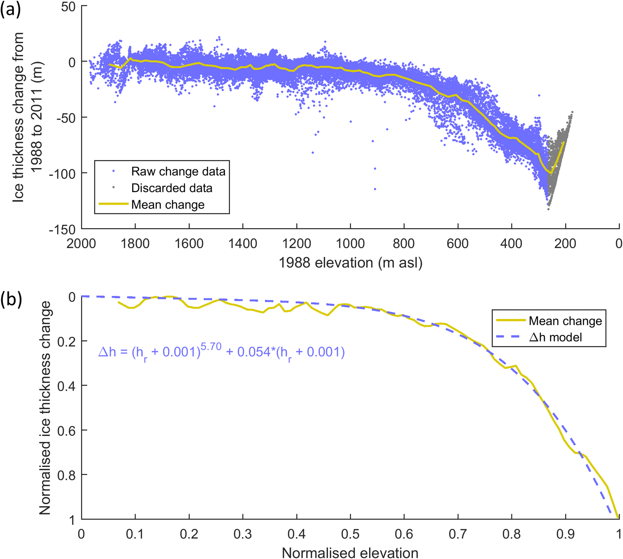
Figure A2 Raw elevation change data from 1988 and 2011 ice DEMs (a) and fitted Δh model to normalised mean elevation change curve following Huss et al. (2010) (b).

In the original formulation by Griffiths et al. (2006), any excess soil water (i.e. when S_soil > TAW) is distributed between overland flow and groundwater recharge pathways. They use a fixed baseflow index (BFI) parameter which defines the proportion of soil water excess that recharges the groundwater. Given the nature of the Virkisá River basin (thin soils overlying impermeable bedrock), it was assumed that soil water migrates to the river outlet only via relatively fast overland flow pathways and so the BFI parameter was set to zero.

A2 Potential evapotranspiration

Potential evapotranspiration can be calculated from measured meteorological data, most simply as a linear function of measured temperature (Blaney and Morin, 1942), or where measurements of wind speed, air pressure and solar radiation exist, the full Penmen–Monteith combination equation can be solved. Given that these additional variables are measured at AWS1 from 2009, the combination equation as defined by Allen et al. (1998) was used to calculate hourly potential evapotranspiration over this period:

$$\begin{array}{}\text{(A2)}& {\mathrm{ET}}_{\mathrm{0}}={\displaystyle \frac{\mathrm{0.408}\mathrm{\Delta }(R_{\mathrm{n}}-G)+\mathit{\gamma }\frac{\mathrm{900}}{T+\mathrm{273}}u(e_{\mathrm{s}}-e_{\mathrm{a}})}{\mathrm{\Delta }+\mathit{\gamma }(\mathrm{1}+\mathrm{0.34}u)}}h,\end{array}$$

where ET₀ is the daily average potential evapotranspiration rate (mm d⁻¹), R_n is the net radiation (MJ m⁻² d⁻¹), G is the soil heat flux (MJ m⁻² d⁻¹), e_s and e_a are the saturation and actual vapour pressure respectively (kPa), Δ is the rate of change in the saturation vapour pressure with temperature (kPa ^∘C⁻¹), γ is the psychrometric constant (kPa ^∘C⁻¹), u is the wind speed (m s⁻¹) and T is the mean daily ambient air temperature (^∘C).

Prior to 2009, the viability of using T as a proxy for ET₀ in a linear regression model framework like Blaney and Morin (1942) was investigated. Similarly, incident solar radiation was also used as the independent variable for this model. In fact, the best fit was achieved using both variables in a multiple linear regression model, which was able to explain 66 % of the ET₀ variance (Fig. A1). This model was used to distribute ET₀ in space and time using the driving temperature and incident solar radiation data.

A3 Glacier geometry evolution

The empirical Δh parametrisation (Huss et al., 2010) requires the availability of at least two digital elevation models of the glacier separated in time. The difference between the two is used to define the Δh polynomial which has the form:

$$\begin{array}{}\text{(A3)}& \mathrm{\Delta }h=(h_{\mathrm{r}}+a{)}^{\mathit{\gamma }}+b(h_{\mathrm{r}}+a)+c,\end{array}$$

where Δh is the normalised surface elevation, h_r is the normalised elevation range and a, b, γ and c are fitted parameters. For this study, the two digital elevation models from 1988 and 2011 were used to define this relationship. Figure A2a shows the raw change data against the 1988 ice elevation. It was decided that the data at the very front of the glacier should not be used, as here the ice has completely melted and as such the bedrock beneath skews the raw change data. Figure A2b shows the Δh model fitted to the normalised mean elevation change curve. Following Huss et al. (2010), the glacier geometry is updated each year by distributing the net glacier mass balance across the glacier according to this relationship.

Appendix B: Temperature lapse rates

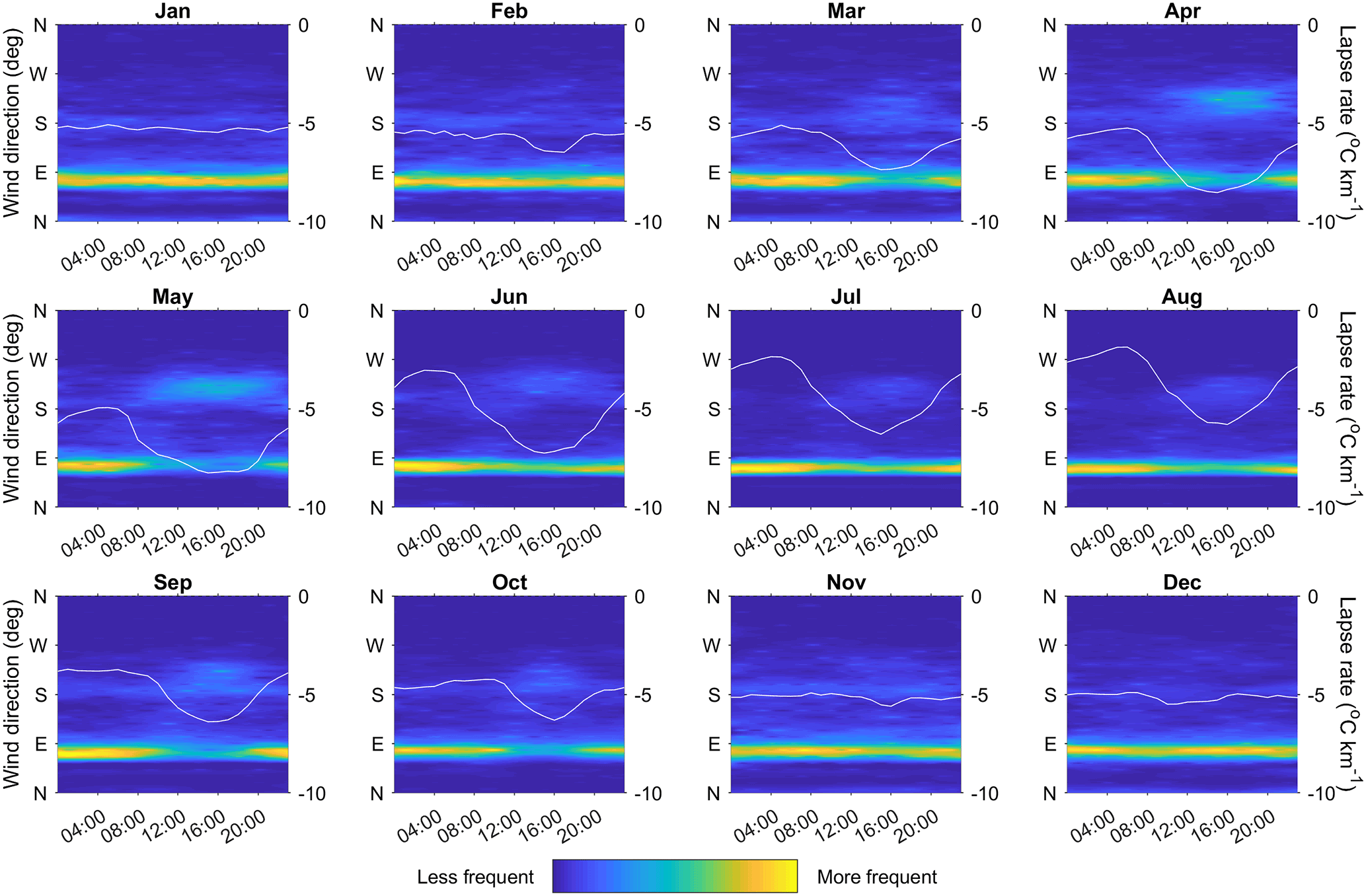
Figure B1 Monthly average hourly temperature lapse rates (white lines, right-hand axis) derived from AWS1 and AWS4 temperature time series overlying heat maps which represent the frequency distribution of hourly wind direction data from AWS4 (left-hand axis).

In order to investigate seasonal variations in lapse rate, the temperature gradient between the lowest (AWS1) and highest (AWS4) weather stations in the Virkisá River basin were analysed. The results showed a remarkable degree of variation in hourly average lapse rate between the months of the year (white lines in Fig. B1). During the winter months between November and February, the lapse rate is relatively stable −5 ^∘C km⁻¹ throughout the day. In contrast, between March and October there is a pronounced diurnal variation in lapse rate that is strongest in the late afternoon and early evening. The heat maps in Fig. B1 represent the frequency distribution of wind direction for each month and show that the development of the strongest lapse rates in the afternoon correspond with a break-up of the prevailing north-easterly winds that flow down from the summit of Öræfajökull and a switch to winds from the south-west. Petersen and Pellicciotti (2011) found a similar phenomenon on the Juncal Norte Glacier in the semi-arid Chilean Andes. They attributed the shallow temperature gradient in the morning to katabatic winds flowing down-glacier, which serve to cool the air over the glacier and weaken the lapse rate. In the afternoon, they showed that a break-up of this layer by valley winds served to increase the temperature gradient by warming the air over the lower glacier. This suggests that winds flowing down from the Öræfajökull summit in the warmer months could serve to cool near-surface air temperatures over the ice, thereby retarding ice melt. To account for this phenomenon, Petersen and Pellicciotti (2011) suggest adopting the Shea and Moore (2010) model to correct on-ice temperatures relative to ambient off-ice weather station measurements. Shea and Moore (2010) found that, for three glaciers on the southern Coast Mountains of British Columbia, Canada, there was a threshold in ambient off-ice air temperature, above which the winds flowing over the glacier served to cool the near-surface on-ice air. They suggest this temperature lies somewhere between 4 and 8 ^∘C but is likely to be site specific.

To investigate whether such a threshold exists on the Virkisjökull glacier, five Gemini Tinytag Aquatic 2 temperature loggers were deployed across the glacier at elevations ranging from 150 to 400 m a.s.l. Each logger was secured at 1.5 m above the ice in a white PVC radiation shield attached to a tripod (Fig. B2). The sensors were deployed for 7 days in late August 2016 and then for a further 7 days in early March 2017 to represent summer and winter on-ice temperatures, respectively. The loggers were synchronised in time with the AWS weather stations and set to measure temperature every 15 min. This allowed for the direct comparison of on- and off-ice near surface temperatures.

Figure B2 Example of Gemini TinyTag housing used for measuring on-ice temperature at one location.

Figure B3 shows the synchronised on- and off-ice temperatures from all of the measurements taken in winter (blue dots) and summer (yellow dots). The off-ice temperatures were derived assuming a linear lapse rate between AWS1 and AWS3 as these are situated at elevations similar to the Tinytag temperature loggers. The results show that there is a temperature threshold above which on-ice temperature falls below off-ice temperature, which was estimated to be 5.27 ^∘C. Following Shea and Moore (2010), Petersen and Pellicciotti (2011), and Ragettli et al. (2014), this cooling effect was interpreted as being due to north-easterly winds which bring cooler air from over the tongue of the glacier, thereby cooling the on-ice air temperature, and the piecewise function derived from Fig. B3 was employed to correct temperatures on the ice during the warmer months when ambient air temperatures exceed this threshold:

$$\begin{array}{}\text{(B1)}& T_{\text{on}}=\left\{\begin{array}{ll}{T}_{\text{off}}& T_{\text{off}}\le \mathrm{5.27}\\ \mathrm{0.74}\cdot T_{\text{off}}+\mathrm{1.38}& T_{\text{off}}>\mathrm{5.27}\end{array}\right.,\end{array}$$

where T_on and T_off are the on- and off-ice near-surface air temperatures (^∘C).

Figure B3 Derived temperature threshold at which on-ice temperature is cooler than the ambient off-ice temperature using the Shea and Moore (2010) model.

Appendix C: Calibration parameters

Table C1 lists all of the calibration parameters for the melt and run-off-routing model structures, which were randomly perturbed during the GHM calibration procedure.

Table C1 Calibration parameters for the melt and run-off-routing model structures.

Appendix D: GHM input/output time series

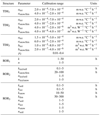
Figure D1 shows the complete GHM input and output time series over the period with observed river discharge data. These include the watershed total precipitation, watershed average temperature and incident solar radiation data used to drive the GHM as well as the simulated watershed total snowmelt, ice melt and river discharge using the TIM₁, TIM₂ and TIM₃ melt model structures in conjunction with the simplest ROR₁ run-off-routing structure. Figure D2 shows the same set of plots when using the ROR₁, ROR₂ and ROR₃ run-off-routing model structures in conjunction with the simplest TIM₁ melt model structure.

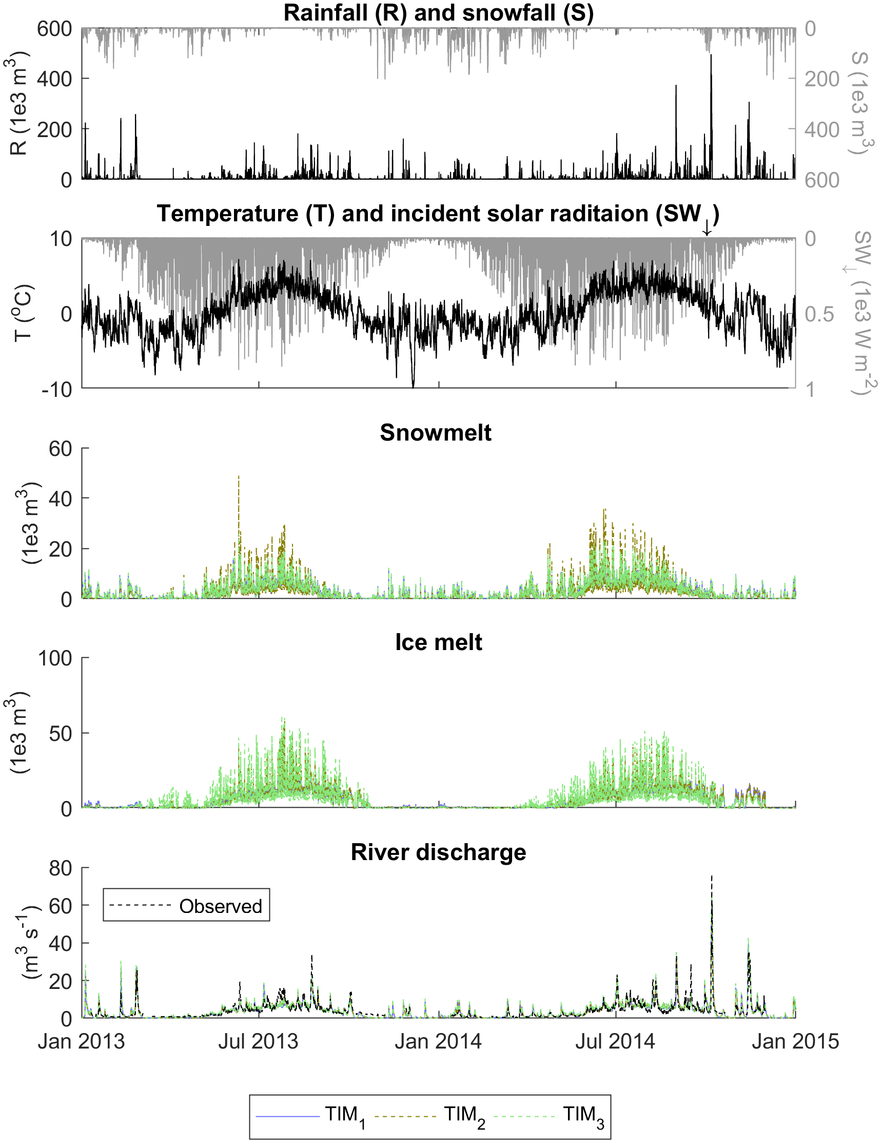
Figure D1 Time series of driving precipitation, temperature and incident solar radiation data and simulated snowmelt, ice melt and river discharge using the TIM₁, TIM₂ and TIM₃ melt model structures in conjunction with the simplest ROR₁ run-off-routing structure. Note that the proportion of rainfall and snowfall is an output from the GHM, which is approximately equal across the different configurations. Ice melt includes melt of bare ice and firn.

Figure D2 Time series of driving precipitation, temperature and incident solar radiation data and simulated snowmelt, ice melt and river discharge using the ROR₁, ROR₂ and ROR₃ run-off-routing model structures in conjunction with the simplest TIM₁ melt model structure. Note that the proportion of rainfall and snowfall is an output from the GHM, which is approximately equal across the different configurations. Also note that ice melt includes melt of bare ice and firn.