Simple analytical–statistical models (ASMs) for mean annual permafrost table temperature and active-layer thickness estimates

A number of models have been developed for estimating the mean annual permafrost table temperature (MAPT) and active-layer thickness (ALT). These tools typically require at least a few ground physical properties as their input parameters in addition to air or ground temperatures. However, ground physical properties are frequently unavailable or unrepresentative and therefore need to be estimated, which introduces uncertainties into model outputs. Hence, we devised two simple analytical–statistical models (ASMs) for MAPT and ALT, which are driven solely by thawing and freezing indices from two depth levels within the active layer, while no ground physical properties are required. ASMs reproduced MAPT and ALT in the Earth's major permafrost regions with the total mean errors of less than 0.05 °C and 9 %, respectively. This is similar or better than other analytical or statistical models, which suggests that ASMs can be useful tools for estimating MAPT and ALT under a wide range of environmental conditions.

1 Introduction

Of ∼ 11 % of the Earth's exposed land surface underlain by permafrost (Obu, 2021), most seasonally thaws from the ground surface to a depth of up to several meters and then completely refreezes, which is mainly controlled by climate conditions and ground physical properties (Bonnaventure and Lamoureux, 2013). This superficial active layer greatly influences the energy and mass transfer between the underlying permafrost, ground surface and the atmosphere, and is therefore critical for the dynamics of hydrological, geomorphic, pedogenic, biological and/or biogeochemical processes including greenhouse gas fluxes, as well as for human infrastructure in permafrost regions (e.g., Grosse et al., 2016; Walvoord and Kurylyk, 2016; Hjort et al., 2022). As climate is a first-order control on ground temperatures and thaw depth (Wang et al., 2019; Smith et al., 2022), the thermal state of permafrost and the thickness of the active layer have attracted a huge interest over recent decades because they are important indicators of how the climate system is evolving (Li et al., 2022; Hrbáček et al., 2023b). Climate change has provoked permafrost warming and active-layer thickening at a global scale (Noetzli et al., 2024; Smith et al., 2024), which can have severe consequences on landscape and ecosystem stability as well as infrastructure integrity. Carbon release due to permafrost degradation is likely to trigger feedback mechanisms with impacts on the Earth's climate system (Lawrence et al., 2015; Schuur et al., 2022). The permafrost and active-layer monitoring is therefore of utmost scientific and societal importance (Brown et al., 2000; Biskaborn et al., 2015).

The thermal state of permafrost and the thickness of the active layer have been investigated by semi-continuous temperature measurements using data loggers with temperature sensors distributed in vertical arrays across the active layer and near-surface permafrost (e.g., Biskaborn et al., 2015; Noetzli et al., 2021), by periodic or semi-continuous geophysical measurements using electric, electromagnetic or seismic methods (e.g., Hauck, 2002; Farzamian et al., 2020), or by periodic thaw-depth measurements using physical probing with rigid rods or thaw-tube readings (e.g., Burn, 1998; Bonnaventure and Lamoureux, 2013). Of these methods, temperature measurements using data loggers are the most convenient in terms of accuracy, temporal resolution and/or logistics, which is well suitable for remote and poorly accessible permafrost regions that have limited or no technical infrastructure (Biskaborn et al., 2015; Streletskiy et al., 2022). However, ground temperatures are frequently measured only in the active layer, and therefore the permafrost temperatures and the active-layer thickness need to be estimated in these situations. This has been done using either statistical methods or numerical and analytical models of various complexity (e.g., Riseborough, 2008; Riseborough et al., 2008; Bonnaventure and Lamoureux, 2013; Aalto et al., 2018).

Of these solutions, analytical models in particular have become popular for estimating the mean annual temperature at the top of permafrost (hereafter referred to as the mean annual permafrost table temperature, MAPT) (Garagulya, 1990; Romanovsky and Osterkamp, 1995; Smith and Riseborough, 1996) and the active-layer thickness (ALT) (Neumann, 1860; Stefan, 1891; Kudryavtsev et al., 1977) because of their simplicity, small number of input parameters, computational efficiency and yet sufficient accuracy, which is advantageous for diverse permafrost regions and environmental settings (e.g., Anisimov et al., 1997; Nelson et al., 1997; Zhao et al., 2017; Obu et al., 2019, 2020). These tools typically require at least a few ground physical properties, such as thermal conductivity, heat capacity, water content or bulk density, as their input parameters in addition to air or ground temperatures. However, ground physical properties are frequently unavailable or unrepresentative and therefore need to be estimated, which introduces uncertainties into model outputs. But even in situ observations of ground physical properties may not guarantee accurate model outputs either, as these properties are usually measured annually or less frequently and are then treated as constants in models, regardless of their temporal variability, which can be considerable (e.g., Gao et al., 2020; Hrbáček et al., 2023a; Li et al., 2023; Kňažková and Hrbáček, 2024; Wenhao et al., 2024).

Here, we devise two novel analytical–statistical models (ASMs) for MAPT and ALT, which are driven solely by thawing and freezing indices from two depth levels within the active layer. ASMs are primarily intended to be used for MAPT or ALT estimates where ground temperature measurements are too shallow and MAPT or ALT therefore cannot be determined directly, while no information on ground physical properties exists. We evaluate ASMs against in situ ground temperature measurements from the Earth's major permafrost regions, and we discuss their performance, advantages and limitations.

2 Model derivation

2.1 Mean annual permafrost table temperature

MAPT [°C] can be calculated using the TTOP model (Romanovsky and Osterkamp, 1995; Smith and Riseborough, 1996), which assumes that the ratio of thawed and frozen thermal conductivity and the effects of latent heat produce the difference between MAPT and the mean annual ground surface temperature (thermal offset). The TTOP formula for permafrost conditions (MAPT ≤ 0 °C) is as follows (Romanovsky and Osterkamp, 1995; Smith and Riseborough, 1996)

$$\begin{array}{}\text{(1)}& \text{MAPT}={\displaystyle \frac{\frac{k_{\mathrm{t}}}{k_{\mathrm{f}}}{I}_{\mathrm{ts}}-I_{\mathrm{fs}}}{P}},\end{array}$$

where k_t [W m⁻¹ K⁻¹] and k_f [W m⁻¹ K⁻¹] is the thawed and frozen thermal conductivity, respectively, that defines the thermal conductivity ratio, I_ts [°C d] and I_fs [°C d] is the ground surface thawing and freezing index, respectively (both assumed in absolute values), and P [365 d] is the length of one year.

However, Eq. (1) can work with thawing and freezing index observed at any depth within the active layer (Riseborough, 2004). This is highly convenient because ground surface temperatures are difficult to measure due to radiative and convective energy fluxes and problematic fixing of temperature sensors exactly at the ground surface (Riseborough, 2003). Using ground temperatures observed at two depth levels within the active layer z₁ and z₂ ($z_{\mathrm{1}}<z_{\mathrm{2}}<$ ALT), MAPT can therefore be expressed as

$$\begin{array}{}\text{(2)}& {\displaystyle }& {\displaystyle }\text{MAPT}={\displaystyle \frac{\frac{k_{\mathrm{t}}}{k_{\mathrm{f}}}{I}_{\mathrm{t}{z}_{\mathrm{1}}}-I_{\mathrm{f}{z}_{\mathrm{1}}}}{P}},\text{(3)}& {\displaystyle }& {\displaystyle }\text{MAPT}={\displaystyle \frac{\frac{k_{\mathrm{t}}}{k_{\mathrm{f}}}{I}_{\mathrm{t}{z}_{\mathrm{2}}}-I_{\mathrm{f}{z}_{\mathrm{2}}}}{P}},\end{array}$$

where $I_{\mathrm{t}{z}_{\mathrm{1}}}$ [°C d] and $I_{\mathrm{f}{z}_{\mathrm{1}}}$ [°C d] is the thawing and freezing index at the depth z₁, and $I_{\mathrm{t}{z}_{\mathrm{2}}}$ [°C d] and $I_{\mathrm{f}{z}_{\mathrm{2}}}$ [°C d] is the thawing and freezing index at the depth z₂. This implies that Eqs. (2) and (3) are equivalent:

$$\begin{array}{}\text{(4)}& {\displaystyle \frac{\frac{k_{\mathrm{t}}}{k_{\mathrm{f}}}{I}_{\mathrm{t}{z}_{\mathrm{1}}}-I_{\mathrm{f}{z}_{\mathrm{1}}}}{P}}={\displaystyle \frac{\frac{k_{\mathrm{t}}}{k_{\mathrm{f}}}{I}_{\mathrm{t}{z}_{\mathrm{2}}}-I_{\mathrm{f}{z}_{\mathrm{2}}}}{P}}.\end{array}$$

Solving Eq. (4) for the thermal conductivity ratio yields

$$\begin{array}{}\text{(5)}& {\displaystyle \frac{k_{\mathrm{t}}}{k_{\mathrm{f}}}}={\displaystyle \frac{I_{\mathrm{f}{z}_{\mathrm{1}}}-I_{\mathrm{f}{z}_{\mathrm{2}}}}{I_{\mathrm{t}{z}_{\mathrm{1}}}-I_{\mathrm{t}{z}_{\mathrm{2}}}}}.\end{array}$$

Equation (5) can be substituted for the thermal conductivity ratio in Eqs. (2) and (3) as follows

$$\begin{array}{}\text{(6)}& {\displaystyle }& {\displaystyle }\text{MAPT}={\displaystyle \frac{\frac{I_{\mathrm{f}{z}_{\mathrm{1}}}-I_{\mathrm{f}{z}_{\mathrm{2}}}}{I_{\mathrm{t}{z}_{\mathrm{1}}}-I_{\mathrm{t}{z}_{\mathrm{2}}}}{I}_{\mathrm{t}{z}_{\mathrm{1}}}-I_{\mathrm{f}{z}_{\mathrm{1}}}}{P}},\text{(7)}& {\displaystyle }& {\displaystyle }\text{MAPT}={\displaystyle \frac{\frac{I_{\mathrm{f}{z}_{\mathrm{1}}}-I_{\mathrm{f}{z}_{\mathrm{2}}}}{I_{\mathrm{t}{z}_{\mathrm{1}}}-I_{\mathrm{t}{z}_{\mathrm{2}}}}{I}_{\mathrm{t}{z}_{\mathrm{2}}}-I_{\mathrm{f}{z}_{\mathrm{2}}}}{P}}.\end{array}$$

Simplifying Eqs. (6) and (7) then produces the same formula for MAPT:

$$\begin{array}{}\text{(8)}& \text{MAPT}={\displaystyle \frac{\frac{I_{\mathrm{f}{z}_{\mathrm{1}}}{I}_{\mathrm{t}{z}_{\mathrm{2}}}-I_{\mathrm{f}{z}_{\mathrm{2}}}{I}_{\mathrm{t}{z}_{\mathrm{1}}}}{I_{\mathrm{t}{z}_{\mathrm{1}}}-I_{\mathrm{t}{z}_{\mathrm{2}}}}}{P}}.\end{array}$$

Substantially, Eq. (8) implies that MAPT can be simply estimated using thawing and freezing indices from two depth levels within the active layer alone, that is, without knowing the thermal conductivity ratio.

Since Eq. (8) was derived from Eq. (1), it has a physical basis (cf. Romanovsky and Osterkamp, 1995). However, it can be shown that it is in principle a linear extrapolation of the freezing index to the depth, where the thawing index becomes zero, and dividing it by the length of one year. Using the same notation as before, this can be expressed as

$$\begin{array}{}\text{(9)}& {\displaystyle }& {\displaystyle \frac{I_{\mathrm{f}{z}_{\mathrm{1}}}-I_{{\mathrm{f}}_{\text{ALT}}}}{I_{\mathrm{t}{z}_{\mathrm{1}}}-I_{{\mathrm{t}}_{\text{ALT}}}}}={\displaystyle \frac{I_{\mathrm{f}{z}_{\mathrm{1}}}-I_{\mathrm{f}{z}_{\mathrm{2}}}}{I_{\mathrm{t}{z}_{\mathrm{1}}}-I_{\mathrm{t}{z}_{\mathrm{2}}}}},\text{(10)}& {\displaystyle }& {\displaystyle \frac{I_{\mathrm{f}{z}_{\mathrm{2}}}-I_{{\mathrm{f}}_{\text{ALT}}}}{I_{\mathrm{t}{z}_{\mathrm{2}}}-I_{{\mathrm{t}}_{\text{ALT}}}}}={\displaystyle \frac{I_{\mathrm{f}{z}_{\mathrm{1}}}-I_{\mathrm{f}{z}_{\mathrm{2}}}}{I_{\mathrm{t}{z}_{\mathrm{1}}}-I_{\mathrm{t}{z}_{\mathrm{2}}}}},\end{array}$$

where $I_{{\mathrm{t}}_{\text{ALT}}}$ [°C d] and $I_{{\mathrm{f}}_{\text{ALT}}}$ [°C d] represents the thawing and freezing index at the base of the active layer. Note that the slope of the relationship is determined by the thermal conductivity ratio. Solving Eqs. (9) and (10) for $I_{{\mathrm{f}}_{\text{ALT}}}$ gives

$$\begin{array}{}\text{(11)}& {\displaystyle }& {\displaystyle }-I_{{\mathrm{f}}_{\text{ALT}}}={\displaystyle \frac{I_{\mathrm{f}{z}_{\mathrm{1}}}-I_{\mathrm{f}{z}_{\mathrm{2}}}}{I_{\mathrm{t}{z}_{\mathrm{1}}}-I_{\mathrm{t}{z}_{\mathrm{2}}}}}\left(I_{\mathrm{t}{z}_{\mathrm{1}}}-I_{{\mathrm{t}}_{\text{ALT}}}\right)-I_{\mathrm{f}{z}_{\mathrm{1}}},\text{(12)}& {\displaystyle }& {\displaystyle }-I_{{\mathrm{f}}_{\text{ALT}}}={\displaystyle \frac{I_{\mathrm{f}{z}_{\mathrm{1}}}-I_{\mathrm{f}{z}_{\mathrm{2}}}}{I_{\mathrm{t}{z}_{\mathrm{1}}}-I_{\mathrm{t}{z}_{\mathrm{2}}}}}\left(I_{\mathrm{t}{z}_{\mathrm{2}}}-I_{{\mathrm{t}}_{\text{ALT}}}\right)-I_{\mathrm{f}{z}_{\mathrm{2}}}.\end{array}$$

Since the thawing index at the base of the active layer is zero, Eqs. (11) and (12) become equivalent to Eqs. (6) and (7), respectively, when divided by the length of one year, and both simplify to Eq. (8). This documents that Eq. (8) can be derived in two alternative manners consisting of analytical and statistical procedures.

2.2 Active-layer thickness

ALT [m] can be calculated using the Stefan (1891) model, which builds on the premise that the conductive heat flux above the thaw front equals to the rate at which latent heat is absorbed as the thaw front propagates downwards. Its simplest form is as follows (Lunardini, 1981)

$$\begin{array}{}\text{(13)}& \text{ALT}=\sqrt{{\displaystyle \frac{\mathrm{2}{k}_{\mathrm{t}}{I}_{\mathrm{ts}}}{L\mathit{\varphi }}}},\end{array}$$

where L [3.34 × 10⁸ J m⁻³] is the volumetric latent heat of fusion of water and ϕ [–] is the volumetric water content. Note that the thawing index must be multiplied by the scaling factor of 86 400 s d⁻¹. As stated previously (Sect. 2.1), ground surface temperatures are difficult to measure (Riseborough, 2003), and therefore the Stefan model has commonly been forced by ground temperatures collected at some depth within the active layer. However, this has rarely been accounted for, although it has been shown to substantially affect the model outputs (Hrbáček and Uxa, 2020; Kaplan Pastíriková et al., 2023). Yet, it can be easily implemented as follows (Riseborough, 2003; Hayashi et al., 2007)

$$\begin{array}{}\text{(14)}& \text{ALT}=z+\sqrt{{\displaystyle \frac{\mathrm{2}{k}_{\mathrm{t}}{I}_{\mathrm{t}z}}{L\mathit{\varphi }}}},\end{array}$$

where z [m] is the depth at which the thawing index I_tz [°C d] is observed. Using ground temperatures observed at two depth levels within the active layer z₁ and z₂ ($z_{\mathrm{1}}<z_{\mathrm{2}}<$ ALT), ALT can therefore be expressed as

$$\begin{array}{}\text{(15)}& {\displaystyle }& {\displaystyle }\text{ALT}=z_{\mathrm{1}}+\sqrt{{\displaystyle \frac{\mathrm{2}{k}_{\mathrm{t}}{I}_{\mathrm{t}{z}_{\mathrm{1}}}}{L\mathit{\varphi }}}},\text{(16)}& {\displaystyle }& {\displaystyle }\text{ALT}=z_{\mathrm{2}}+\sqrt{{\displaystyle \frac{\mathrm{2}{k}_{\mathrm{t}}{I}_{\mathrm{t}{z}_{\mathrm{2}}}}{L\mathit{\varphi }}}}.\end{array}$$

This implies that Eqs. (15) and (16) are equivalent:

$$\begin{array}{}\text{(17)}& z_{\mathrm{1}}+\sqrt{{\displaystyle \frac{\mathrm{2}{k}_{\mathrm{t}}{I}_{\mathrm{t}{z}_{\mathrm{1}}}}{L\mathit{\varphi }}}}=z_{\mathrm{2}}+\sqrt{{\displaystyle \frac{\mathrm{2}{k}_{\mathrm{t}}{I}_{\mathrm{t}{z}_{\mathrm{2}}}}{L\mathit{\varphi }}}}.\end{array}$$

The vertical distance between z₂ and z₁ can be expressed as

$$\begin{array}{}\text{(18)}& z_{\mathrm{2}}-z_{\mathrm{1}}=\sqrt{{\displaystyle \frac{\mathrm{2}{k}_{\mathrm{t}}{I}_{\mathrm{t}{z}_{\mathrm{1}}}}{L\mathit{\varphi }}}}-\sqrt{{\displaystyle \frac{\mathrm{2}{k}_{\mathrm{t}}{I}_{\mathrm{t}{z}_{\mathrm{2}}}}{L\mathit{\varphi }}}},\end{array}$$

which simplifies to

$$\begin{array}{}\text{(19)}& z_{\mathrm{2}}-z_{\mathrm{1}}=\sqrt{{\displaystyle \frac{\mathrm{2}{k}_{\mathrm{t}}}{L\mathit{\varphi }}}}\left(\sqrt{I_{\mathrm{t}{z}_{\mathrm{1}}}}-\sqrt{I_{\mathrm{t}{z}_{\mathrm{2}}}}\right).\end{array}$$

Subsequently rearranging Eq. (19) gives

$$\begin{array}{}\text{(20)}& {\displaystyle \frac{z_{\mathrm{2}}-z_{\mathrm{1}}}{\sqrt{I_{\mathrm{t}{z}_{\mathrm{1}}}}-\sqrt{I_{\mathrm{t}{z}_{\mathrm{2}}}}}}=\sqrt{{\displaystyle \frac{\mathrm{2}{k}_{\mathrm{t}}}{L\mathit{\varphi }}}},\end{array}$$

where the right-hand side corresponds to the so-called edaphic term (Nelson and Outcalt, 1987), which has been used to combine the thawed thermal conductivity and volumetric water content into a single variable in the modified Stefan model:

$$\begin{array}{}\text{(21)}& \text{ALT}=E\sqrt{I_{\mathrm{ts}}},\end{array}$$

where E [m °C^−0.5 d^−0.5] denotes the edaphic term given by

$$\begin{array}{}\text{(22)}& E=\sqrt{{\displaystyle \frac{\mathrm{2}{k}_{\mathrm{t}}}{L\mathit{\varphi }}}}.\end{array}$$

Although Eq. (21) is equivalent to Eq. (13), it has frequently been preferred for estimating ALT because the edaphic term can be calibrated based on the relationship between ALT and thawing index, that is, without knowing the thawed thermal conductivity and volumetric water content (Nelson and Outcalt, 1987; Hinkel and Nicholas, 1995; Nelson et al., 1997; Anisimov et al., 2002; Shiklomanov and Nelson, 2002; Smith et al., 2009; Shiklomanov et al., 2010; Peng et al., 2023). The edaphic term can be implemented in Eqs. (15) and (16) as follows

$$\begin{array}{}\text{(23)}& {\displaystyle }& {\displaystyle }\text{ALT}=z_{\mathrm{1}}+E\sqrt{I_{\mathrm{t}{z}_{\mathrm{1}}}},\text{(24)}& {\displaystyle }& {\displaystyle }\text{ALT}=z_{\mathrm{2}}+E\sqrt{I_{\mathrm{t}{z}_{\mathrm{2}}}}.\end{array}$$

Substituting the left-hand side of Eq. (20) for the edaphic term in Eqs. (23) and (24) yields

$$\begin{array}{}\text{(25)}& {\displaystyle }& {\displaystyle }\text{ALT}=z_{\mathrm{1}}+{\displaystyle \frac{z_{\mathrm{2}}-z_{\mathrm{1}}}{\sqrt{I_{\mathrm{t}{z}_{\mathrm{1}}}}-\sqrt{I_{\mathrm{t}{z}_{\mathrm{2}}}}}}\sqrt{I_{\mathrm{t}{z}_{\mathrm{1}}}},\text{(26)}& {\displaystyle }& {\displaystyle }\text{ALT}=z_{\mathrm{2}}+{\displaystyle \frac{z_{\mathrm{2}}-z_{\mathrm{1}}}{\sqrt{I_{\mathrm{t}{z}_{\mathrm{1}}}}-\sqrt{I_{\mathrm{t}{z}_{\mathrm{2}}}}}}\sqrt{I_{\mathrm{t}{z}_{\mathrm{2}}}}.\end{array}$$

Simplifying Eqs. (25) and (26) then produces the same formula for ALT:

$$\begin{array}{}\text{(27)}& \text{ALT}={\displaystyle \frac{z_{\mathrm{2}}\sqrt{I_{\mathrm{t}{z}_{\mathrm{1}}}}-z_{\mathrm{1}}\sqrt{I_{\mathrm{t}{z}_{\mathrm{2}}}}}{\sqrt{I_{\mathrm{t}{z}_{\mathrm{1}}}}-\sqrt{I_{\mathrm{t}{z}_{\mathrm{2}}}}}}.\end{array}$$

Substantially, Eq. (27) implies that ALT can be simply estimated using thawing indices from two depth levels within the active layer alone, that is, without knowing the thawed thermal conductivity and volumetric water content or the edaphic term.

Since Eq. (27) was derived from Eq. (13), it has a physical basis (cf. Lunardini, 1981). However, it can also be shown that it is in principle a linear extrapolation of the depth where the square root of the thawing index becomes zero (cf. Riseborough, 2003). This can be expressed as

$$\begin{array}{}\text{(28)}& {\displaystyle }& {\displaystyle \frac{\text{ALT}-z_{\mathrm{1}}}{\sqrt{I_{\mathrm{t}{z}_{\mathrm{1}}}}-\sqrt{I_{{\mathrm{t}}_{\text{ALT}}}}}}={\displaystyle \frac{z_{\mathrm{2}}-z_{\mathrm{1}}}{\sqrt{I_{\mathrm{t}{z}_{\mathrm{1}}}}-\sqrt{I_{\mathrm{t}{z}_{\mathrm{2}}}}}},\text{(29)}& {\displaystyle }& {\displaystyle \frac{\text{ALT}-z_{\mathrm{2}}}{\sqrt{I_{\mathrm{t}{z}_{\mathrm{2}}}}-\sqrt{I_{{\mathrm{t}}_{\text{ALT}}}}}}={\displaystyle \frac{z_{\mathrm{2}}-z_{\mathrm{1}}}{\sqrt{I_{\mathrm{t}{z}_{\mathrm{1}}}}-\sqrt{I_{\mathrm{t}{z}_{\mathrm{2}}}}}}.\end{array}$$

Note that the slope of the relationship is determined by the edaphic term. Solving Eqs. (28) and (29) for ALT gives

$$\begin{array}{}\text{(30)}& {\displaystyle }& {\displaystyle }\text{ALT}=z_{\mathrm{1}}+{\displaystyle \frac{z_{\mathrm{2}}-z_{\mathrm{1}}}{\sqrt{I_{\mathrm{t}{z}_{\mathrm{1}}}}-\sqrt{I_{\mathrm{t}{z}_{\mathrm{2}}}}}}\left(\sqrt{I_{\mathrm{t}{z}_{\mathrm{1}}}}-\sqrt{I_{{\mathrm{t}}_{\text{ALT}}}}\right),\text{(31)}& {\displaystyle }& {\displaystyle }\text{ALT}=z_{\mathrm{2}}+{\displaystyle \frac{z_{\mathrm{2}}-z_{\mathrm{1}}}{\sqrt{I_{\mathrm{t}{z}_{\mathrm{1}}}}-\sqrt{I_{\mathrm{t}{z}_{\mathrm{2}}}}}}\left(\sqrt{I_{\mathrm{t}{z}_{\mathrm{2}}}}-\sqrt{I_{{\mathrm{t}}_{\text{ALT}}}}\right).\end{array}$$

Since the thawing index at the base of the active layer is zero, Eqs. (30) and (31) are equivalent to Eqs. (25) and (26), respectively, and both simplify to Eq. (27). As with Eq. (8), this documents that Eq. (27) can also be derived in two alternative manners consisting of analytical and statistical procedures.

3 Model evaluation

ASMs for estimating MAPT and ALT were evaluated using in situ ground temperature measurements from the Earth's major permafrost regions that differ in climate, permafrost zone, ground surface cover and/or ground physical properties and their distribution within the active layer to enhance the robustness of the model evaluation. Unlike manual thaw-depth measurements, such as those from the Circumpolar Active Layer Monitoring (CALM) network (Brown et al., 2000), ground temperature measurements with sensors distributed in vertical arrays across the active layer and near-surface permafrost provide high temporal and depth resolutions, which enable consistent determination of MAPT and ALT using a uniform procedure at all sites and ensure the homogeneity of the validation dataset. Since the accuracy of these MAPT and ALT values depends on the spacing of the ground temperature sensors (Riseborough, 2003, 2008), we attempted to keep their maximum distances at 25 and 50 cm for ALT of <1 and >1 m, respectively. While this requirement excluded numerous sites, it ensured that the benchmark values for MAPT and ALT could be established as accurately as possible.

We collected ground temperature data for a total of 55 sites from monitoring networks and public databases of the Polar-Geo-Lab of the Masaryk University (MU) (e.g., Hrbáček et al., 2017a, b; Hrbáček and Uxa, 2020; Hrbáček et al., 2025), Global Terrestrial Network for Permafrost (GTN-P; http://gtnpdatabase.org, last access: 20 November 2024), Natural Resources Conservation Service of the United States Department of Agriculture (USDA; https://www.nrcs.usda.gov/resources/data-and-reports/soil-climate-research-stations, last access: 19 September 2024), Geophysical Institute Permafrost Laboratory of the University of Alaska Fairbanks (GI-UAF, https://permafrost.gi.alaska.edu, last access: 25 July 2025), Yukon Permafrost Database (YPD, https://service.yukon.ca/permafrost/, last access: 25 July 2025), Nordicana D of the Centre for Northern Studies (ND, https://nordicana.cen.ulaval.ca/en/, last access: 15 July 2025), and National Tibetan Plateau/Third Pole Environment Data Center (NTP/TPEDC; https://data.tpdc.ac.cn/en/disallow/789e838e-16ac-4539-bb7e-906217305a1d, last access: 21 November 2024) (Zhao et al., 2021). The dataset comprised five different ground surface covers and four permafrost zones, spanned variable time periods during 1997–2023, and exhibited a wide range of MAPT and ALT from $\sim -\mathrm{19}$ to ∼ 0 °C and ∼ 40 to ∼ 310 cm, respectively (Table C1).

Ground temperature data were first checked for quality and then daily means were calculated for all available depths before further processing. Thawing and freezing indices were calculated as annual sums of positive and negative mean daily ground temperatures, respectively, which were expressed in absolute values for convenience. Following standard procedures and monitoring guidelines (Streletskiy et al., 2022), ALT was determined as the maximum annual depth of the 0 °C isotherm that was tracked by linear interpolation of mean daily ground temperatures within the measured profile. MAPT was calculated as the mean annual ground temperature, which was linearly interpolated to the depth that corresponds to ALT (e.g., Hrbáček et al., 2020, 2021; Kňažková and Hrbáček, 2024). It is important to note that there is no universal method for interpolating between ground temperature sensors that works best, and therefore we used the linear interpolation, which is generally accepted (e.g., Streletskiy et al., 2022). Hereafter, these values are referred to as the observed MAPT and ALT. They were considered suitable for the model evaluation because ∼ 65 % of the observed MAPT differed by less than 0.1 °C from the temperature of the closest temperature sensor used for the interpolation and ∼ 80 % of the observed ALT were less than 10 cm from the closest temperature sensor, which sets their maximum possible deviations from the actual MAPT and ALT values (Fig. 1).

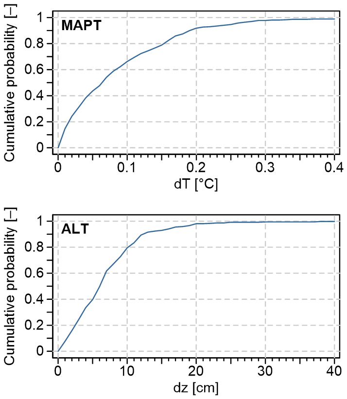
Figure 1 Cumulative distributions of the temperature and depth differences between the observed MAPT and ALT and the closest temperature sensor used for the linear interpolation, which sets their maximum possible deviations from the actual MAPT and ALT values.

Subsequently, MAPT and ALT were also modelled using ASMs given by Eqs. (8) and (27) forced by the observed thawing and freezing indices from the depth intervals of 0–10, 25–35 and 45–55 cm, which were combined into three pairs of $\mathrm{5}/\mathrm{30}$, $\mathrm{5}/\mathrm{50}$ and $\mathrm{30}/\mathrm{50}$ cm so that they were comparable across the validation sites. This provided us with three sets of MAPT and ALT estimates that allowed to determine which depth combinations worked best. The three depth pairs were situated within the active layer in all instances, and therefore differed from the temperature sensors used to determine the observed MAPT and ALT, so this did not invalidate the evaluation.

We compared the modelled MAPT and ALT directly with the observed MAPT and ALT, and evaluated the model accuracy for each site using common error metrics, such as mean error (ME), mean percentage error (MPE), mean absolute error (MAE), mean absolute percentage error (MAPE), and root-mean-square error (RMSE). The evaluation statistics were grouped by depth pairs and surface cover, as the latter also broadly captures the common characteristics of the validation sites in terms of climate and composition of the active layer.

4 Results

4.1 Mean annual permafrost table temperature

The MAPT modelled using ASM given by Eq. (8) based on the observed thawing and freezing indices for the depth pairs of $\mathrm{5}/\mathrm{30}$, $\mathrm{5}/\mathrm{50}$ and $\mathrm{30}/\mathrm{50}$ cm showed the total site-weighted ME from 0.01 °C to 0.05 °C compared to the observed MAPT (Table 1). Since the errors were scattered around zero (Fig. 2), the total site-weighted MAE was somewhat larger and ranged from 0.11 to 0.16 °C, while the total site-weighted RMSE was 0.12 to 0.19 °C (Table 1). The majority of errors were well within ±0.2 °C (Fig. 2).

Table 1 Evaluation statistics of MAPT modelled using ASM given by Eq. (8) based on the observed thawing and freezing indices for the depth pairs of $\mathrm{5}/\mathrm{30}$, $\mathrm{5}/\mathrm{50}$ and $\mathrm{30}/\mathrm{50}$ cm and diverse surface covers.

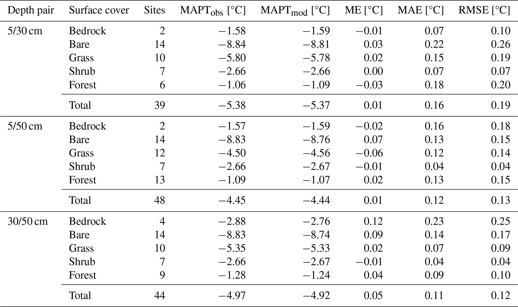
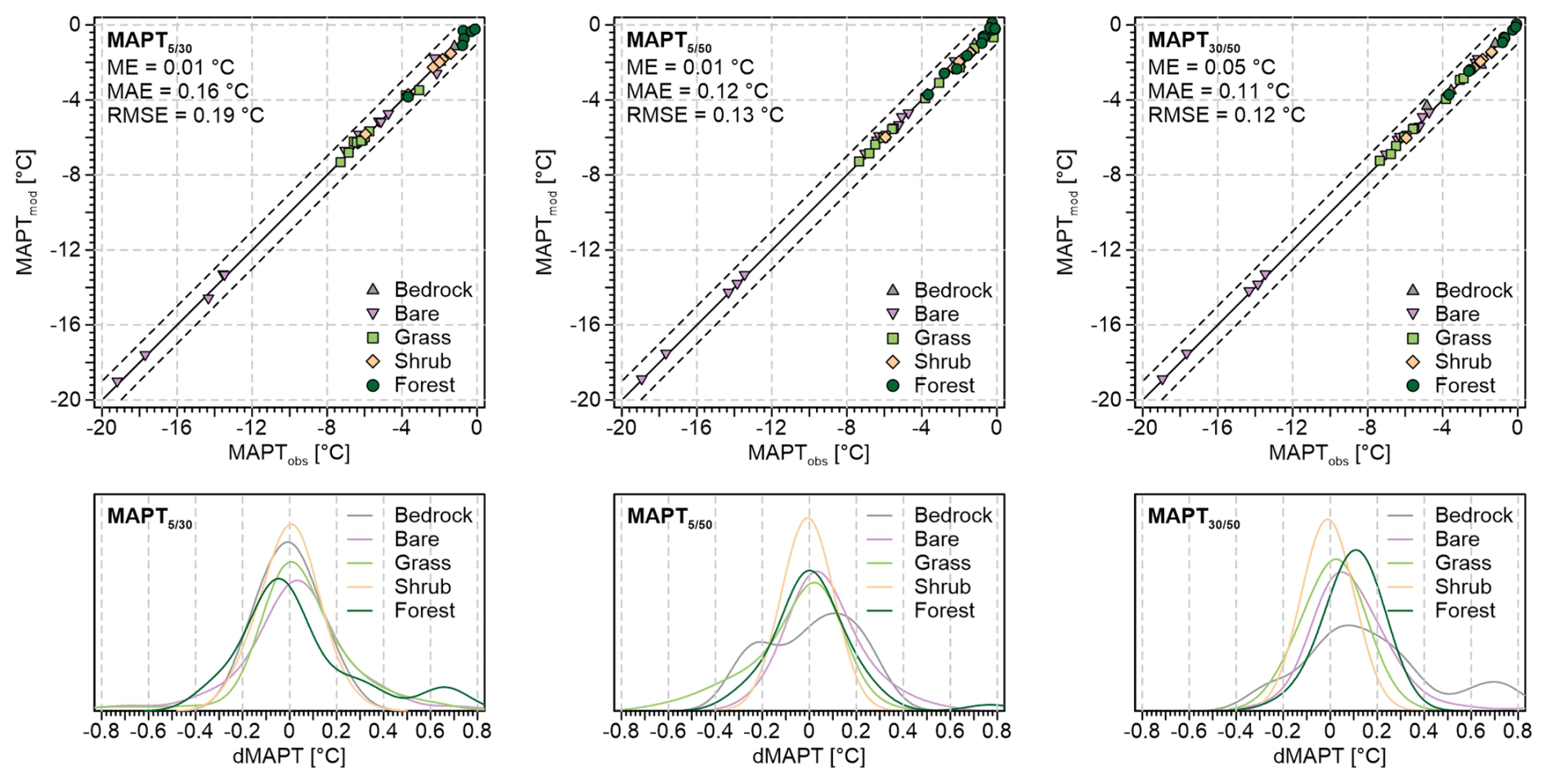
Figure 2 Comparison of the observed MAPT and MAPT modelled using ASM given by Eq. (8) based on the observed thawing and freezing indices for the depth pairs of $\mathrm{5}/\mathrm{30}$, $\mathrm{5}/\mathrm{50}$ and $\mathrm{30}/\mathrm{50}$ cm and diverse surface covers. The black solid and dashed lines in the upper plots represent the line of identity and the deviation of ±1 °C, respectively.

The accuracy of the modelled MAPT was similar for the three depth pairs, although $\mathrm{5}/\mathrm{50}$ and $\mathrm{30}/\mathrm{50}$ cm performed slightly better than 5/30 cm (Table 1). Similarly, there were rather small differences between individual surface covers (Fig. 2) that exhibited the site-weighted ME from −0.06 to 0.12 °C (Table 1). However, the MAPT estimates were somewhat better at the vegetated sites, as the site-weighted MAE and RMSE there were mostly less than ∼ 0.15 °C, while the bedrock and bare-ground sites mostly showed the site-weighted MAE and RMSE greater than ∼ 0.15 °C (Table 1). The site-weighted errors also tended to be somewhat larger at higher MAPT for all three depth pairs.

4.2 Active-layer thickness

The ALT modelled using ASM given by Eq. (27) based on the observed thawing indices for the depth pairs of $\mathrm{5}/\mathrm{30}$, $\mathrm{5}/\mathrm{50}$ and $\mathrm{30}/\mathrm{50}$ cm exhibited the total site-weighted ME from −11.5 cm (−9.3 %) to −1.6 cm (−1.2 %) compared to the observed ALT (Table 2). The total site-weighted MAE was larger (Fig. 3) and reached 13.1 cm (10.2 %) to 17.1 cm (19.8 %), while the total site-weighted RMSE was 14.2 cm to 18.2 cm (Table 2).

Table 2 Evaluation statistics of ALT modelled using ASM given by Eq. (27) based on the observed thawing and freezing indices for the depth pairs of $\mathrm{5}/\mathrm{30}$, $\mathrm{5}/\mathrm{50}$ and $\mathrm{30}/\mathrm{50}$ cm and diverse surface covers.

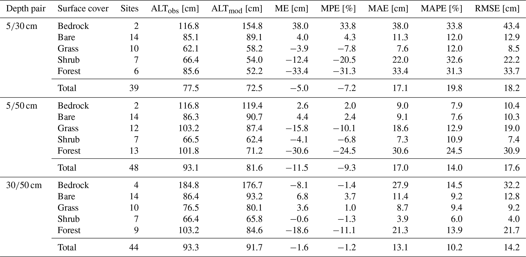
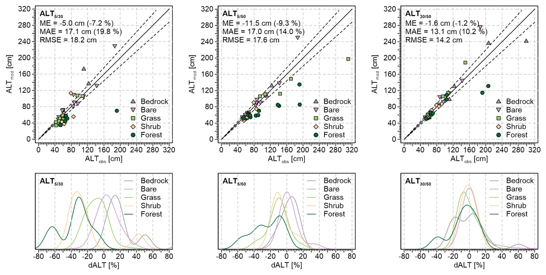
Figure 3 Comparison of the observed ALT and ALT modelled using ASM given by Eq. (27) based on the observed thawing and freezing indices for the depth pairs of $\mathrm{5}/\mathrm{30}$, $\mathrm{5}/\mathrm{50}$ and $\mathrm{30}/\mathrm{50}$ cm and diverse surface covers. The black solid and dashed lines in the upper plots represent the line of identity and the deviation of ±10 %, respectively.

The accuracy of the modelled ALT was higher for the depth pairs of $\mathrm{5}/\mathrm{50}$ and $\mathrm{30}/\mathrm{50}$ cm compared to $\mathrm{5}/\mathrm{30}$ cm, especially at the bedrock, shrub and forest sites (Table 2). Additionally, there were rather large differences between individual surface covers (Fig. 3), among which the site-weighted ME ranged from −33.4 cm (−31.3 %) to 38.0 cm (33.8 %) (Table 2). The most accurate ALT estimates were at the bare-ground sites and those with grass and shrub cover, as their site-weighted MAE ranged from 3.9 cm (6.0 %) to 22.0 cm (32.6 %), and the site-weighted RMSE was from 4.0 cm to 22.2 cm (Table 2). Somewhat worse was the model performance at the bedrock and forest sites, with the site-weighted MAE from 9.0 cm (7.9 %) to 38.0 cm (33.8 %) and the site-weighted RMSE from 10.4 cm to 43.4 cm (Table 2). The site-weighted errors were also larger at thicker ALT for all three depth pairs.

5 Discussion

5.1 Mean annual permafrost table temperature

The modelled MAPT showed a relatively high accuracy for all three depth pairs and surface covers (Fig. 2), with the mean errors close to zero and the majority of them within ±0.2 °C (Table 1), which is similar or better than in most previous studies that used other analytical or statistical models for MAPT (e.g., Romanovsky and Osterkamp, 1995; Sazonova and Romanovsky, 2003; Ferreira et al., 2017; Way and Lewkowicz, 2018; Wang et al., 2020; Kaplan Pastíriková et al., 2023).

Somewhat larger errors in the modelled MAPT arose especially under warmer conditions and within a thicker active layer where MAPT needs to be extrapolated to greater depth. Warmer climates are also dominated by vegetated sites (Table C1) with well-developed soils and therefore a more heterogeneous active layer where MAPT estimates are more difficult. In addition, it may also be associated with increased complexity of the system at permafrost temperatures approaching 0 °C when simple models tend to fail to a greater extent (Riseborough, 2007). The worst MAPT estimates at the bedrock sites were also likely because active layer is thick there (Table 1). Moreover, the boreholes were drilled into vertical rockwalls, and therefore it is possible that lateral flows of heat and moisture occur in the fractured bedrock, which further complicates MAPT estimates.

So far, models for estimating MAPT have typically assumed that the ratio of thawed and frozen thermal conductivity is less than or equal to 1, and that the thermal offset is therefore negative (e.g., Gisnås et al., 2013; Obu et al., 2019, 2020), which would result in invalid MAPT estimates if the actual conditions were reversed. However, although nearly half of the bedrock and bare-ground sites exhibited a positive thermal offset with a thermal conductivity ratio above 1, the MAPT was modelled with similar accuracy at these locations as elsewhere (Table 1, Fig. 2). This is because ASM utilizes thawing and freezing indices within the active layer and can therefore easily capture this behaviour. This is also demonstrated by the thermal conductivity ratios modelled using Eq. (5) for the three depth pairs that are close to those determined for the whole active layer (Fig. 4) based on the relationship between MAPT and thawing and freezing indices (Riseborough, 2004; Way and Lewkowicz, 2018). This is likely because the relationship between the thawing and freezing indices within the active layer is linear (see Sect. 2.1) and its slope varies rather slightly with vertical changes in ground physical properties.

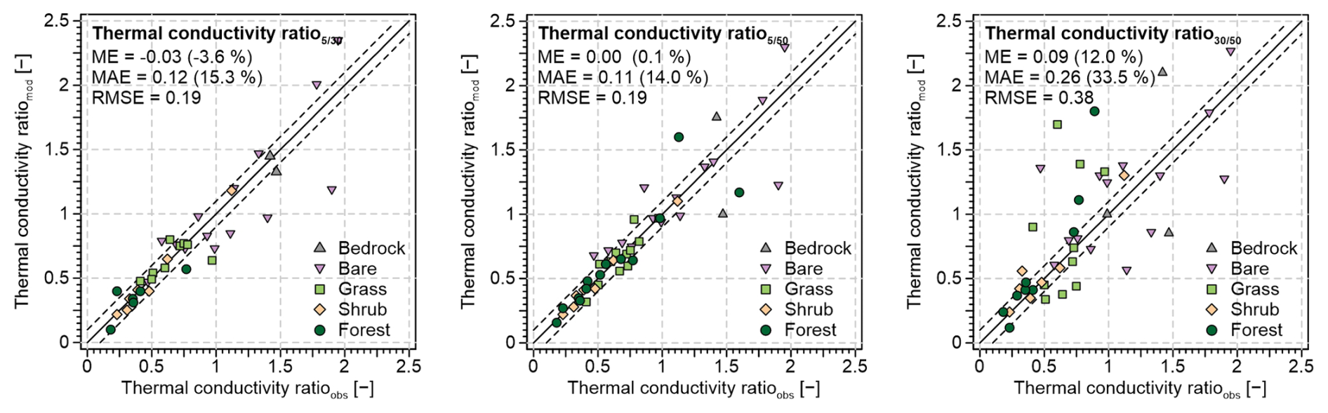
Figure 4 Comparison of the thermal conductivity ratio for the whole active layer determined using the rearranged Eq. (2) based on the observed MAPT and the observed thawing and freezing indices for the uppermost available sensors (Riseborough, 2004; Way and Lewkowicz, 2018) and the thermal conductivity ratio estimated using Eq. (5) based on the observed thawing and freezing indices for the depth pairs of $\mathrm{5}/\mathrm{30}$, $\mathrm{5}/\mathrm{50}$ and $\mathrm{30}/\mathrm{50}$ cm and diverse surface covers. The black solid and dashed lines represent the line of identity and the deviation of ±0.1.

5.2 Active-layer thickness

Unlike MAPT, the modelled ALT showed variable performance for individual depth pairs and surface covers (Fig. 3, Table 2). However, the errors were mostly well within ±20 %, which is also similar or better than in most previous studies that used other analytical or statistical models for ALT (Anisimov et al., 1997; Nelson et al., 1997; Romanovsky and Osterkamp, 1997; Anisimov et al., 2002; Shiklomanov and Nelson, 2002; Sazonova and Romanovsky, 2003; Streletskiy et al., 2012; Yin et al., 2016; Zorigt et al., 2016; Hrbáček and Uxa, 2020; Kaplan Pastíriková et al., 2023).

Notably, the modelled ALT showed variable accuracy for the depth pair of $\mathrm{5}/\mathrm{30}$ cm (Table 2). This is because the active layer is typically more heterogeneous at the vegetated sites and may often comprise a surface organic layer there, the physical properties of which strongly differ from the ground underneath. This alters the temperature gradient within the active layer and results in worse ALT estimates, which can be observed especially at the shrub and forest sites (Fig. 3). By contrast, the ALT estimates showed substantially lower errors for the depth pairs of $\mathrm{5}/\mathrm{50}$ and $\mathrm{30}/\mathrm{50}$ cm (Fig. 3), which largely to completely eliminated the influence of the surface layer. This also explains the consistently high accuracy of the modelled ALT at the bare-ground sites for all three depth pairs (Table 2), as the active layer there is relatively homogeneous in terms of its stratigraphy and physical properties. The ALT estimates were also relatively accurate at the bedrock sites (Table 2), but the same concern exists for them as for MAPT (see Sect. 5.1). Similarly to MAPT, the modelled ALT tended to be less accurate under warmer conditions dominated by vegetated sites with a more heterogeneous and thick active layer (Table C1) where ALT needs to be extrapolated to greater depth.

Previous studies have estimated the edaphic term based on the relationship between ALT and thawing index (Nelson and Outcalt, 1987; Hinkel and Nicholas, 1995; Nelson et al., 1997; Anisimov et al., 2002; Shiklomanov and Nelson, 2002; Smith et al., 2009; Shiklomanov et al., 2010; Strand et al., 2021; Xu and Wu, 2021; Peng et al., 2023), which is restrictive because it requires ALT. However, the edaphic term modelled using Eq. (20) for the three depth levels was close to the edaphic term determined for the whole active layer (Fig. 5) based on the relationship between ALT and thawing index (Nelson and Outcalt, 1987; Hinkel and Nicholas, 1995). As with MAPT, this is because the square root of the thawing index within the active layer is linear (see Sect. 2.2) and its slope varies rather slightly with vertical changes in ground physical properties (Riseborough, 2003).

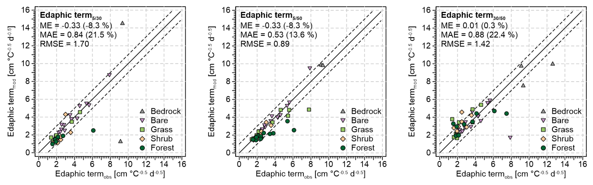
Figure 5 Comparison of the observed edaphic term for the whole active layer determined using the rearranged Eq. (23) based on the observed ALT and the observed thawing index for the uppermost available sensor (Nelson and Outcalt, 1987; Hinkel and Nicholas, 1995) and the edaphic term estimated using Eq. (20) based on the observed thawing indices for the depth pairs of $\mathrm{5}/\mathrm{30}$, $\mathrm{5}/\mathrm{50}$ and $\mathrm{30}/\mathrm{50}$ cm and diverse surface covers. The black solid and dashed lines represent the line of identity and the deviation of ± 1 cm °C^−0.5 d^−0.5.

5.3 Model advantages

Unlike other analytical or statistical models for MAPT (e.g., Garagulya, 1990; Romanovsky and Osterkamp, 1995; Smith and Riseborough, 1996) and ALT (e.g., Neumann, 1860; Stefan, 1891; Kudryavtsev et al., 1977), ASMs given by Eqs. (8) and (27) can work in any grounds where conductive heat transfer prevails without knowing their physical properties.

Although ASMs utilize only thawing and freezing indices from two depth levels within the active layer as inputs, they inherently account for the natural variability of ground physical properties in the intermediate layer between these two depths that is expressed in terms of annual and seasonal means of the thermal conductivity ratio and the edaphic term, respectively. Similarly, ASMs consider latent and sensible heat or other factors that influence the thermal regime between the two depth levels, although these effects are not explicitly accounted for. This is because the relative values of the thawing and freezing indices at the two depth levels reflect the rate of heat transfer in the intermediate layer between them (see Eqs. 5 and 20) that is influenced by seasonal changes in ground physical properties. So in principle it is analogous to, for instance, the calculations of apparent thermal diffusivity, which are based on damping of temperature amplitude or phase lag between two depth levels (Horton et al., 1983).

This is highly convenient because ground physical properties, such as thermal conductivity, heat capacity, water content or bulk density, are frequently unavailable or unrepresentative. Ground physical properties in other models for MAPT and ALT have therefore been estimated empirically or based on published values with unknown validity (e.g., Hinkel and Nicholas, 1995; Nelson et al., 1997; Anisimov et al., 2002; Shiklomanov and Nelson, 2002; Gisnås et al., 2013; Obu et al., 2019, 2020; Garibaldi et al., 2021). Ground physical properties also show more or less variability on seasonal and annual time scales (e.g., Gao et al., 2020; Hrbáček et al., 2023a; Li et al., 2023; Kňažková and Hrbáček, 2024; Wenhao et al., 2024), which most other models cannot handle because they typically treat ground physical properties as constants for whole modelling periods. Of course, ASMs also treat them as constants, but their values are annual or seasonal means that reflect the variations in ground physical properties over time mainly due to changes in water content and as such they are representative for individual years or thawing seasons. This is a major improvement over other analytical or statistical models for MAPT (e.g., Garagulya, 1990; Romanovsky and Osterkamp, 1995; Smith and Riseborough, 1996) and ALT (e.g., Neumann, 1860; Stefan, 1891; Kudryavtsev et al., 1977), which can increase the spatial and/or temporal validity of modelled MAPT and ALT.

Moreover, we believe that, in addition to MAPT and ALT estimates, ASMs can also be useful for investigating the spatial and temporal variations in the thermal conductivity ratio (Fig. 4) and the edaphic term (Fig. 5) regardless of MAPT and ALT (cf. Nelson and Outcalt, 1987; Hinkel and Nicholas, 1995; Riseborough, 2004; Way and Lewkowicz, 2018). This could be done using networks of miniature temperature loggers collecting data only in shallow parts of the active layer because another advantage of ASMs is that their inputs can be any depth combinations from within the active layer. For most accurate outputs, however, we suggest using thawing and freezing indices from depth levels as close as possible to the permafrost table. For instance, this could improve ALT estimates at the bedrock sites where active layer is thick.

In addition to in situ ground temperature measurements, we suppose that ASMs could also be forced by diverse climate reanalyses or Earth system models, if these at least partially account for the physics of ground thawing and freezing. While these products have been widely used for permafrost applications (e.g., Cao et al., 2020; Kaplan Pastíriková et al., 2025; Liu et al., 2025), they typically provide only ground surface and shallow active-layer temperatures with ground physical properties largely unknown, which is frequently insufficient to determine MAPT and ALT directly or using conventional models. If the active layer is thick, MAPT and ALT have therefore usually been confined to the deepest ground temperature level available in these products, which can obviously be misleading (e.g., Cao et al., 2020). However, ASMs are designed so that they should be able to provide MAPT and ALT estimates even under these conditions.

Lastly, ASMs can also be easily reformulated to be used for estimating the mean annual temperature at the base of seasonally frozen ground and frost depth (see Appendices A and B).

5.4 Model limitations

Since ASMs assume that active layer is vertically homogeneous, they can be biased if there are strong vertical changes in ground physical properties and/or higher ground-ice content near the base of the active layer (Riseborough, 2003). For instance, if temperature measurements are used from the topmost layer, whose physical properties differ from the rest of the active layer, ASMs may be inaccurate. Similarly, the modelled MAPT and ALT may be unreliable if only shallow temperature measurements in a thick active layer are used. This is because the estimates would be based on physical properties of a small portion of the active layer, which may be different in its deeper parts. Nevertheless, the natural variability of ground physical properties without sharp changes in their vertical distribution is unlikely to have a major influence on the MAPT and ALT estimates (see Figs. 2 and 3, Tables 1 and 2).

Other downside of ASMs is that they require temperature measurements from two depth levels within the active layer, which may not be available at many sites.

6 Conclusions

We devised two novel analytical–statistical models (ASMs) for estimating MAPT and ALT given by Eqs. (8) and (27), respectively, which are driven solely by thawing and freezing indices from two depth levels within the active layer, while no ground physical properties are required. ASMs reproduced MAPT and ALT in the Earth's major permafrost regions with the total mean errors of less than 0.05 °C and 9 %, respectively, which is very promising because it is similar or better than other analytical or statistical models. ASMs worked best in a homogeneous active layer with small vertical changes in ground physical properties and when permafrost table was close below the temperature sensors considered for MAPT and ALT estimates. By contrast, they performed worst in a heterogeneous and thick active layer when the topmost organic layer influenced the estimates.

We believe that ASMs can find useful applications under a wide range of climates, ground surface covers and ground physical conditions wherever at least two temperature measurements within the active layer are available. They are primarily intended to be used for MAPT or ALT estimates where ground temperature measurements are too shallow and MAPT or ALT therefore cannot be determined directly, but they can also be used to establish typical values of the thermal conductivity ratio and the edaphic term for MAPT and ALT estimates in the past and in the future or for modelling their spatial variations. In addition to in situ measurements, they could utilize diverse climate reanalyses or Earth system models. Lastly, they can be easily reformulated for estimating the mean annual temperature at the base of seasonally frozen ground and frost depth.

Appendix A: Derivation of ASM for mean annual temperature at the base of seasonally frozen ground

Similarly to Eq. (1), the mean annual temperature at the base of seasonally frozen ground (MASFT > 0 °C) is calculated as follows (Romanovsky and Osterkamp, 1995)

$$\begin{array}{}\text{(A1)}& \text{MASFT}={\displaystyle \frac{I_{\mathrm{ts}}-\frac{k_{\mathrm{f}}}{k_{\mathrm{t}}}{I}_{\mathrm{fs}}}{P}}.\end{array}$$

MASFT based on temperatures observed at two distinct depths in the seasonally freezing layer z₁ and z₂ ($z_{\mathrm{1}}<z_{\mathrm{2}}<$ FD) can therefore be expressed as follows

$$\begin{array}{}\text{(A2)}& {\displaystyle }& {\displaystyle }\text{MASFT}={\displaystyle \frac{I_{\mathrm{t}{z}_{\mathrm{1}}}-\frac{k_{\mathrm{f}}}{k_{\mathrm{t}}}{I}_{\mathrm{f}{z}_{\mathrm{1}}}}{P}},\text{(A3)}& {\displaystyle }& {\displaystyle }\text{MASFT}={\displaystyle \frac{I_{\mathrm{t}{z}_{\mathrm{2}}}-\frac{k_{\mathrm{f}}}{k_{\mathrm{t}}}{I}_{\mathrm{f}{z}_{\mathrm{2}}}}{P}}.\end{array}$$

This implies that Eqs. (A2) and (A3) are equivalent:

$$\begin{array}{}\text{(A4)}& {\displaystyle \frac{I_{\mathrm{t}{z}_{\mathrm{1}}}-\frac{k_{\mathrm{f}}}{k_{\mathrm{t}}}{I}_{\mathrm{f}{z}_{\mathrm{1}}}}{P}}={\displaystyle \frac{I_{\mathrm{t}{z}_{\mathrm{2}}}-\frac{k_{\mathrm{f}}}{k_{\mathrm{t}}}{I}_{\mathrm{f}{z}_{\mathrm{2}}}}{P}}.\end{array}$$

Solving Eq. (A4) for the inverse of the thermal conductivity ratio yields

$$\begin{array}{}\text{(A5)}& {\displaystyle \frac{k_{\mathrm{f}}}{k_{\mathrm{t}}}}={\displaystyle \frac{I_{\mathrm{t}{z}_{\mathrm{1}}}-I_{\mathrm{t}{z}_{\mathrm{2}}}}{I_{\mathrm{f}{z}_{\mathrm{1}}}-I_{\mathrm{f}{z}_{\mathrm{2}}}}}.\end{array}$$

Equation (A5) can be then substituted for the thermal conductivity ratio in Eqs. (A2) and (A3) as follows

$$\begin{array}{}\text{(A6)}& {\displaystyle }& {\displaystyle }\text{MASFT}={\displaystyle \frac{I_{\mathrm{t}{z}_{\mathrm{1}}}-\frac{I_{\mathrm{t}{z}_{\mathrm{1}}}-I_{\mathrm{t}{z}_{\mathrm{2}}}}{I_{\mathrm{f}{z}_{\mathrm{1}}}-I_{\mathrm{f}{z}_{\mathrm{2}}}}{I}_{\mathrm{f}{z}_{\mathrm{1}}}}{P}},\text{(A7)}& {\displaystyle }& {\displaystyle }\text{MASFT}={\displaystyle \frac{I_{\mathrm{t}{z}_{\mathrm{2}}}-\frac{I_{\mathrm{t}{z}_{\mathrm{1}}}-I_{\mathrm{t}{z}_{\mathrm{2}}}}{I_{\mathrm{f}{z}_{\mathrm{1}}}-I_{\mathrm{f}{z}_{\mathrm{2}}}}{I}_{\mathrm{f}{z}_{\mathrm{2}}}}{P}}.\end{array}$$

Subsequently, Eqs. (A6) and (A7) both simplify to the same formula for MASFT:

$$\begin{array}{}\text{(A8)}& \text{MASFT}={\displaystyle \frac{\frac{I_{\mathrm{f}{z}_{\mathrm{1}}}{I}_{\mathrm{t}{z}_{\mathrm{2}}}-I_{\mathrm{f}{z}_{\mathrm{2}}}{I}_{\mathrm{t}{z}_{\mathrm{1}}}}{I_{\mathrm{f}{z}_{\mathrm{1}}}-I_{\mathrm{f}{z}_{\mathrm{2}}}}}{P}},\end{array}$$

which only slightly differs from Eq. (8).

Appendix B: Derivation of ASM for frost depth

Similarly to Eq. (13), the frost depth (FD) can be calculated using the Stefan (1891) model as follows

$$\begin{array}{}\text{(B1)}& \text{FD}=\sqrt{{\displaystyle \frac{\mathrm{2}{k}_{\mathrm{f}}{I}_{\mathrm{fs}}}{L\mathit{\varphi }}}}.\end{array}$$

As with Eq. (13), note that the freezing index must be multiplied by the scaling factor of 86 400 s d⁻¹. FD estimated using freezing indices observed at two distinct depths z₁ and z₂ ($z_{\mathrm{1}}<z_{\mathrm{2}}<$ FD) can be expressed as follows

$$\begin{array}{}\text{(B2)}& {\displaystyle }& {\displaystyle }\text{FD}=z_{\mathrm{1}}+\sqrt{{\displaystyle \frac{\mathrm{2}{k}_{\mathrm{f}}{I}_{\mathrm{f}{z}_{\mathrm{1}}}}{L\mathit{\varphi }}}},\text{(B3)}& {\displaystyle }& {\displaystyle }\text{FD}=z_{\mathrm{2}}+\sqrt{{\displaystyle \frac{\mathrm{2}{k}_{\mathrm{f}}{I}_{\mathrm{f}{z}_{\mathrm{2}}}}{L\mathit{\varphi }}}}.\end{array}$$

This implies that Eqs. (B2) and (B3) are equivalent:

$$\begin{array}{}\text{(B4)}& z_{\mathrm{1}}+\sqrt{{\displaystyle \frac{\mathrm{2}{k}_{\mathrm{f}}{I}_{\mathrm{f}{z}_{\mathrm{1}}}}{L\mathit{\varphi }}}}=z_{\mathrm{2}}+\sqrt{{\displaystyle \frac{\mathrm{2}{k}_{\mathrm{f}}{I}_{\mathrm{f}{z}_{\mathrm{2}}}}{L\mathit{\varphi }}}}.\end{array}$$

The vertical distance between z₂ and z₁ can be expressed as

$$\begin{array}{}\text{(B5)}& z_{\mathrm{2}}-z_{\mathrm{1}}=\sqrt{{\displaystyle \frac{\mathrm{2}{k}_{\mathrm{f}}{I}_{\mathrm{f}{z}_{\mathrm{1}}}}{L\mathit{\varphi }}}}-\sqrt{{\displaystyle \frac{\mathrm{2}{k}_{\mathrm{f}}{I}_{\mathrm{f}{z}_{\mathrm{2}}}}{L\mathit{\varphi }}}},\end{array}$$

which simplifies to

$$\begin{array}{}\text{(B6)}& z_{\mathrm{2}}-z_{\mathrm{1}}=\sqrt{{\displaystyle \frac{\mathrm{2}{k}_{\mathrm{f}}}{L\mathit{\varphi }}}}\left(\sqrt{I_{\mathrm{f}{z}_{\mathrm{1}}}}-\sqrt{I_{\mathrm{f}{z}_{\mathrm{2}}}}\right).\end{array}$$

Subsequently rearranging Eq. (B6) gives

$$\begin{array}{}\text{(B7)}& {\displaystyle \frac{z_{\mathrm{2}}-z_{\mathrm{1}}}{\sqrt{I_{\mathrm{f}{z}_{\mathrm{1}}}}-\sqrt{I_{\mathrm{f}{z}_{\mathrm{2}}}}}}=\sqrt{{\displaystyle \frac{\mathrm{2}{k}_{\mathrm{f}}}{L\mathit{\varphi }}}},\end{array}$$

where the right-hand side corresponds to the edaphic term, which combines the ground physical properties in the Stefan model into a single variable. The edaphic term can be implemented in Eqs. (B2) and (B3) as

$$\begin{array}{}\text{(B8)}& {\displaystyle }& {\displaystyle }\text{FD}=z_{\mathrm{1}}+E\sqrt{I_{\mathrm{f}{z}_{\mathrm{1}}}},\text{(B9)}& {\displaystyle }& {\displaystyle }\text{FD}=z_{\mathrm{2}}+E\sqrt{I_{\mathrm{f}{z}_{\mathrm{2}}}}.\end{array}$$

Substituting the left-hand side of Eq. (B7) for the edaphic term in Eqs. (B8) and (B9) yields

$$\begin{array}{}\text{(B10)}& {\displaystyle }& {\displaystyle }\text{FD}=z_{\mathrm{1}}+{\displaystyle \frac{z_{\mathrm{2}}-z_{\mathrm{1}}}{\sqrt{I_{\mathrm{f}{z}_{\mathrm{1}}}}-\sqrt{I_{\mathrm{f}{z}_{\mathrm{2}}}}}}\sqrt{I_{\mathrm{f}{z}_{\mathrm{1}}}},\text{(B11)}& {\displaystyle }& {\displaystyle }\text{FD}=z_{\mathrm{2}}+{\displaystyle \frac{z_{\mathrm{2}}-z_{\mathrm{1}}}{\sqrt{I_{\mathrm{f}{z}_{\mathrm{1}}}}-\sqrt{I_{\mathrm{f}{z}_{\mathrm{2}}}}}}\sqrt{I_{\mathrm{f}{z}_{\mathrm{2}}}}.\end{array}$$

Simplifying Eqs. (B10) and (B11) then produces the same formula for FD:

$$\begin{array}{}\text{(B12)}& \text{FD}={\displaystyle \frac{z_{\mathrm{2}}\sqrt{I_{\mathrm{f}{z}_{\mathrm{1}}}}-z_{\mathrm{1}}\sqrt{I_{\mathrm{f}{z}_{\mathrm{2}}}}}{\sqrt{I_{\mathrm{f}{z}_{\mathrm{1}}}}-\sqrt{I_{\mathrm{f}{z}_{\mathrm{2}}}}}},\end{array}$$

which is the same as Eq. (27), but with the freezing indices instead of the thawing ones.

Appendix C

Table C1 List of sites used for model evaluation.

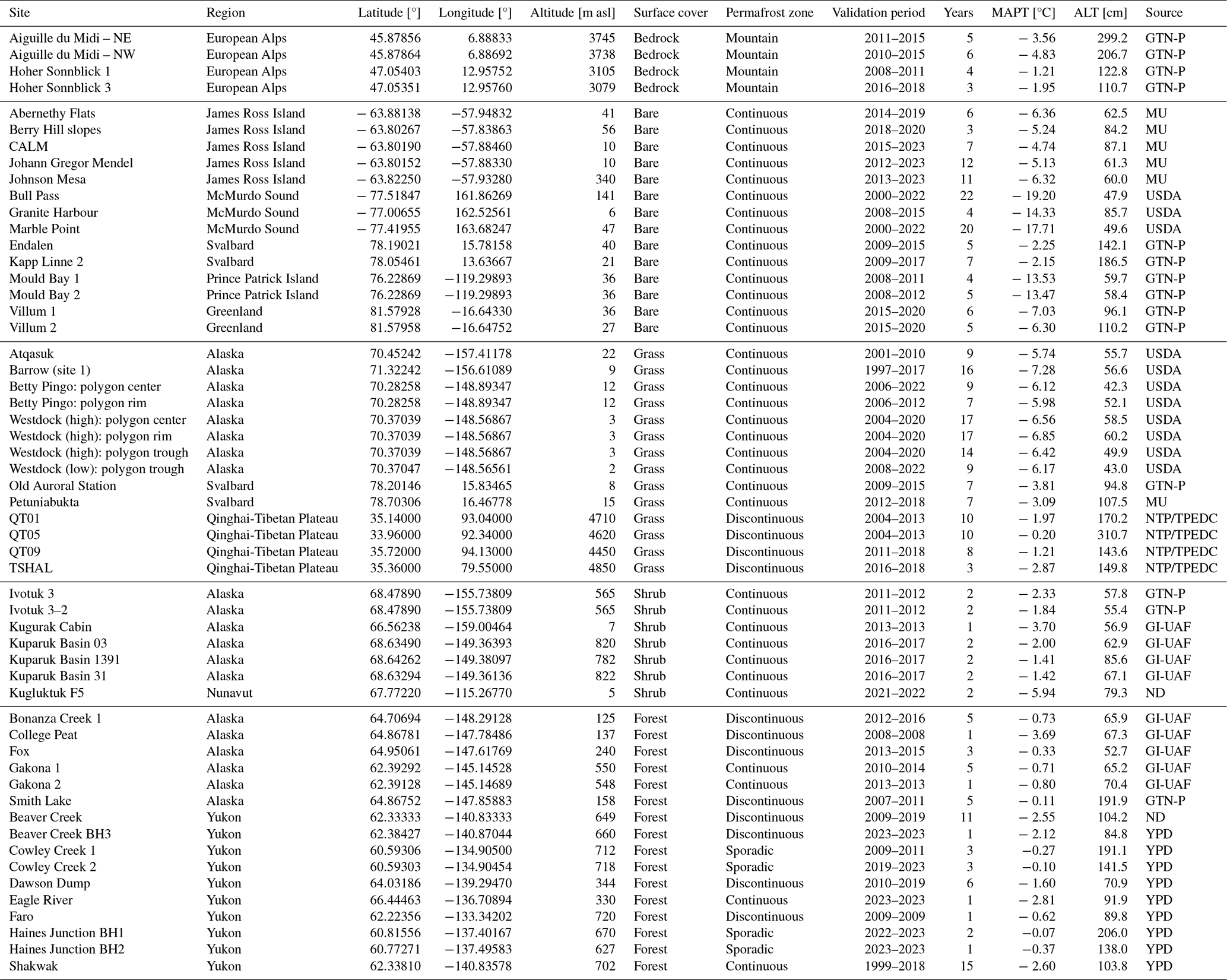
GTN-P = Global Terrestrial Network for Permafrost, MU = Polar-Geo-Lab of the Masaryk University, USDA = Natural Resources Conservation Service of the United States Department of Agriculture, NTP/TPEDC = National Tibetan Plateau/Third Pole Environment Data Center, GI-UAF = Geophysical Institute Permafrost Laboratory of the University of Alaska Fairbanks, ND = Nordicana D of the Centre for Northern Studies, YPD = Yukon Permafrost Database.