Antarctic ice sheet model comparison with uncurated geological constraints shows that higher spatial resolution improves deglacial reconstructions

Accurately reconstructing past changes to the shape and volume of the Antarctic ice sheet relies on the use of physically based and thus internally consistent ice sheet modeling, benchmarked against spatially limited geologic data. The challenge in model benchmarking against geologic data is diagnosing whether model-data misfits are the result of an inadequate model, inherently noisy or biased geologic data, and/or incorrect association between modeled quantities and geologic observations. In this work we address this challenge by (i) the development and use of a new model-data evaluation framework applied to an uncurated data set of geologic constraints, and (ii) nested high-spatial-resolution modeling designed to test the hypothesis that model resolution is an important limitation in matching geologic data. While previous approaches to model benchmarking employed highly curated datasets, our approach applies an automated screening and quality control algorithm to an uncurated public dataset of geochronological observations (specifically, cosmogenic-nuclide exposure-age measurements from glacial deposits in ice-free areas). This optimizes data utilization by including more geological constraints, reduces potential interpretive bias, and allows unsupervised assimilation of new data as they are collected. We also incorporate a nested model framework in which high-resolution domains are downscaled from a continent-wide ice sheet model. We highlight the application of this framework by applying these methods to a small ensemble of deglacial ice-sheet model simulations, and demonstrate that the nested approach improves the ability of model simulations to match exposure age data collected from areas of complex topography and ice flow. We develop a range of diagnostic model-data comparison metrics to provide more insight into model performance than possible from a single-valued misfit statistic, showing that different metrics capture different aspects of ice sheet deflation.

1 Introduction

The overall goal of this study is to improve the ability to benchmark ice sheet model simulations against direct geological constraints of ice sheet behavior during the last ∼ 20 000 years. Broadly, it is important to evaluate the performance and accuracy of ice sheet models using the geologic record because these models are used to project future ice sheet change and consequent sea-level impacts. Because the time period of direct or remotely sensed observations of ice sheet variability is too short to adequately benchmark models of ice sheet processes operating on decadal to millennial timescales, the use of geologic data is necessary. Geologic records from across the Antarctic continent provide critical information about past ice sheet behavior, especially during the last glacial cycle, but are spatially and temporally sparse and discontinuous, so cannot by themselves produce a quantitative estimate of deglacial sea level contribution. Reconstructing past changes in the shape and volume of the entire ice sheet, therefore, relies on the use of physically based ice sheet models to interpolate sparse data and find internally consistent ice sheet change histories that match the data. Used together, models and data can provide a robust and physically based reconstruction of glacial evolution. Geologically validated simulations of the last glacial cycle are necessary for quantifying Antarctica's contribution to deglacial sea level rise in the past, providing a loading history and glacioisotatic boundary conditions for models that aim to predict future ice sheet change and sea-level impacts, and understanding the likely accuracy of these predictions.

Here we develop and implement a model-data comparison framework for deglacial ice-sheet behavior recorded by Antarctic terrestrial geologic data that record ice sheet thinning. Specifically, the majority of geological evidence for LGM-to-present thinning of the Antarctic ice sheet consists of cosmogenic-nuclide exposure-age data from glacially transported clasts collected from ice-free areas throughout Antarctica. These clasts are first exposed to cosmic ray flux when uncovered by ice thinning; thus, a number of clasts collected at a range of elevations across a nunatak site produce an age-elevation array in which clasts at higher elevations were uncovered first and therefore have older exposure ages.

This work follows several previous seminal efforts to benchmark ice sheet models against geological data. Briggs and Tarasov (2013) compiled a relatively small and highly curated dataset consisting of about 200 geologically based constraints on past ice thickness (from cosmogenic-nuclide exposure-dating), past ice sheet extent, and past relative sea level; developed model-data evaluation metrics; and applied their constraint database to score an ensemble of ice sheet model simulations (Briggs et al., 2014). Pollard et al. (2016) took a similar approach, adding more data (from a curated community dataset of geologic constraints binned into 5 kyr timeslices; The RAISED Consortium et al., 2014) and exploring more advanced statistical approaches for evaluating model-data fit. Pittard et al. (2022) build on this existing framework for evaluating Antarctic-wide model simulations using a database of geologic constraints, implementing modern-day elimination sieves and past ice-area metrics with the ultimate goal of producing an ice history to drive models of glacial isostatic adjustment. Lecavalier et al. (2023) further curate and expand the Briggs and Tarasov (2013) constraint dataset, incorporating more recent literature as well as new data types (for example, borehole temperature from ice cores), and then applying this new curated dataset to a large ensemble of model simulations (Lecavalier and Tarasov, 2025). Ely et al. (2019) complement these Antarctic-wide model scoring exercises with a “timing accordance” tool to evaluate ice sheet model output compared to a user-prepared gridded geochronological dataset recording the timing of ice presence/absence across the region of interest.

Overall, these studies provided a foundation for this work by establishing good practices for model-data misfit calculations, but relied extensively on manual inspection, interpretation, and curation of geologic data, which potentially introduces interpretive bias and, more importantly, does not allow for assimilation of new data as the available geologic data set grows rapidly. Furthermore, prior efforts have relied heavily on modern-day misfits for scoring model ensembles. Here we expand on previous model-data comparison efforts by:

Replacing manual data curation with an inclusive automated methodology. Previous work has employed manual curation of geologic datasets to ensure that each model constraint provides a robust metric for comparison. A highly curated approach is effective for eliminating outliers and erroneous or unphysical data points, but it only utilizes a fraction of the extensive (though often imperfect) geologic records that currently exist, and it also can potentially introduce interpretation bias. In addition, assimilation of newly collected data in an internally consistent way requires that the original curator regularly revise the data set, which, in general, has not been feasible in the past. Here we attempt an opposite approach, with algorithms that utilize the ICE-D exposure-age database, an inclusive, publicly available database of terrestrial geologic constraints that is continuously updated as these data are collected.

We develop automated methodologies for data selection and processing to replace manual curation: for example, at a terrestrial site with cosmogenic nuclides, we establish a set of processing steps and consistent criteria for systematically selecting samples that record the last deglaciation rather than previous ones (see Sect. 3.4) or identifying a limit on maximum ice thickness above present (Sect. 4.3).

The advantages of this uncurated, inclusive approach are that (i) all known data can be used to inform our understanding about deglacial ice sheet behavior; and (ii) newly collected data can immediately be assimilated into the constraint data set. The key potential disadvantage is that the processing algorithm has a less than 100 % success rate at identifying samples that would likely be interpreted as outliers or errors by manual curation. It is hard to know the true significance of this effect, because manual curation, even by experts, will also very likely accept some erroneous data. An additional feature of our approach, however, is therefore to accept that some fraction of the constraint data set is spurious or aberrant, and design model-data comparison strategies to prevent a single pathological site from having an outsize impact on model scoring (see Sect. 4.2.4).

Providing publicly available and easily updated geologic model constraint datasets. Our approach is publicly available, allowing user interaction and customization via a GHub tool (https://theghub.org/tools/modeldatathin with open access code and model output). Users can access the static dataset of geologic constraints extracted from the public ICE-D database on 24 April 2024 and used in this paper (see Code and Data Availability statement), or re-query and re-compute updated datasets through the GHub tool (as well as customize the model-data scoring parameters). Our flexible framework allows the geologic model constraint database to evolve with the emergence of new data.

Focusing on paleo geologic data rather than present-day misfits. Here we focus on reconstructing ice sheet dynamics through the last deglaciation as recorded solely by geologic data, deliberately omitting present-day ice thickness and ice extent misfits. Modern ice thickness and velocity fields have high spatial resolution, complete spatial coverage, low measurement uncertainty, and low structural uncertainty; by contrast, paleo data are patchily distributed in space and time, with significant measurement and structural uncertainties. This disproportionality in the extent and quality of present-day vs. paleo data has the tendency to bias model evaluation towards fitting the present-day rather than past data. For example, in Briggs and Tarasov (2013) where model scores are weighted by data type, 83 % of a model score reflects the modern misfit (compared to 2 % from marine grounding line retreat age, 7 % from terrestrial thinning, and 8 % from RSL records). As another approach, Pittard et al. (2022) simulations that do not pass a modern-day ice configuration “sieve” are eliminated even before they are scored against geologic data. Here, we shift the focus to the Holocene behavior of the ice sheet, isolating model fit to only the paleo geologic data in order to specifically investigate ice sheet dynamics through the last deglaciation. Although we do not use the modern ice sheet configuration to directly score model results, we note that model members with patently incorrect modern configurations still score poorly against the paleo-data (discussed below).

Implementing nested ice sheet modeling to achieve unprecedented resolution. Exposure age data are collected from rock outcrops, generally in mountainous regions of steep topography characterized by complex flow evolution and multiple interacting glaciers throughout the last glacial cycle. In these areas with significant topographic variation (e.g., mountainous regions), bed elevation, ice thickness, and ice velocity can vary at much smaller spatial scales than can be represented in coarse-resolution (typically 20 km or larger) continental-scale ice sheet models. In fact, there are many sites where exposure-age data were collected adjacent to very large, 10–20-km-wide glaciers that drain significant portions of the ice sheet, but are not resolved as glaciers at all in continental-scale models with 20 km or larger grid cells.

When glacier systems are below the model grid resolution, dynamic thinning is not captured. In other words, a model grid cell that should be acting like a glacier flowing through topography is instead acting like an isolated icefield sitting on top of a topographic high. In this situation, it is not reasonably possible for the model simulation to match the data. Thus, ice dynamics are often very different between model simulations and reality, which means that coarse-resolution models are most likely simply incapable of matching exposure age reconstructions of local ice thickness variations at many sites, except by accident.

Many sites are located at the transition from streaming ice to interior thinning, and very different thinning rates have been observed across short distances. This complexity cannot be represented by coarser-resolution models (Mas e Braga et al., 2021), where glacier thinning records are generally compared to modeled ice elevation along glacier centerlines or at glacier mouths (Hillebrand et al., 2021), or averaged ice thickness changes across large coastal regions (Lowry et al., 2019). Furthermore, thinning occurs faster along the centerline of glaciers compared to the flanks (Pritchard et al., 2009); thus, exposure age dates may reflect delayed thinning of the ice-marginal areas, which can only be investigated at a high resolution.

Previous work has relied on continental-scale ice sheet models at 40 km (Briggs and Tarasov, 2013; Lecavalier and Tarasov, 2025) or 20 km (Pollard et al., 2016 over West Antarctica only; Pittard et al., 2022) to compare against mountain-side-transect ice thinning measurements. Thus, each of these preceding studies have grappled with the model resolution issue in various ways. For example, Pittard et al. (2022) de-weighted exposure age sites located in complex topography, reducing the constraining value of these datasets. Briggs and Tarasov (2013) apply a vertical uncertainty to each model thinning curve that reflects the ice thickness difference at a site that can be induced by a coarse resolution grid: they compare ice thickness in a modern 5 km gridded ice sheet product versus a downscaled version at 40 km. Lecavalier and Tarasov (2025) widen their spatial consideration to also include thinning profiles in neighboring (40 km) grid cells around a site. Similarly, although Lowry et al. (2019) do not quantitatively score their model simulations against cosmogenic nuclide data, they compare exposure age thinning profiles at various sites against a modeled regional average of ice thickness change across hundreds of km (rather than identifying the precise grid cell registered to each exposure age site).

Here, we implement high-resolution (2 km) nested ice sheet model domains, spanning all locations where exposure age data have been collected across the continent, to better resolve ice sheet thinning and complex flow patterns across high-relief topography. This enables model-data comparison at an order-of-magnitude higher resolution than previous studies.

Quantifying multiple diagnostic metrics for model-data fit. Here we develop and describe multiple model-data evaluation metrics that highlight different aspects of deglacial ice sheet evolution. For example, assessing terrestrial thinning patterns using past ice elevations above modern, a standard approach, blends together a model simulation's ability to reproduce the amplitude, timing, and rate of deglaciation at a site. While all of these aspects are important characteristics of deglaciation, if we wanted to specifically investigate events of rapid ice-sheet change, for example (such as abrupt terrestrial thinning during the mid-Holocene; Jones et al., 2022, and refs therein), we might want to prioritize model fidelity to the rate and/or timing of reconstructed ice sheet thinning while de-emphasizing fit to the absolute magnitude of thickness change. Isolating a particular component of model-data fit provides a targeted strategy for addressing different specific scientific questions and improving understanding of what processes in the model might be responsible for misfits.

In this paper, we describe the development and deployment of our model-data comparison toolkit. We first discuss the modeling techniques that we apply towards this goal, including the underlying choices that shape the simulation and extraction of model deglacial history for comparison with geologic data (Sect. 2). In Sect. 3, we describe the geologic dataset used here – cosmogenic nuclide measurements – and the acquisition and processing of raw data. We then introduce our automated methodology for identifying youngest age-elevation bounding samples and discuss our treatment of sample uncertainty. Having extracted analogous thinning profiles from both geologic datasets and model simulations, we develop and present two key methods to capture different aspects of model-data fit (Sect. 4.1). We investigate the impacts of our methodological choices and describe our formulation of model data fit (Sect. 4.2), formalizing two model-data assessment metrics (Sect. 4.2.2). In addition to the exposure-age dataset of thinning constraints, we also compile an exposure-age dataset of maximum-thickness constraints, comprised of sites where exposure age measurements bracket the local last-glacial-cycle ice thickness change. This secondary dataset also leverages cosmogenic nuclide measurements but applies them to constrain the maximum ice thickness achieved during the last glacial cycle. We correspondingly develop an independent model-data metric to evaluate the modeled amplitude of ice thickness changes (Sect. 4.3).

With these scoring techniques in hand, we apply our model-data framework to the small ensemble of numerical ice-sheet model simulations (Sect. 5). Model scores using our uncurated and automated sample selection methods are compared to model scores using a recent comprehensive curated dataset (Sect. 5.1) to ensure that we have not introduced any systematic failures in our approach by eliminating manual curation. We also investigate the impact of model grid resolution on model-data fit by comparing results from continental simulations to nested high-resolution model domains (Sect. 5.2), showing that these high-resolution nested domains indeed improve model representation of ice thinning patterns across mountainous terrestrial regions where exposure-age data are often collected. In Sect. 6, we synthesize and interpret our multiple metrics for model-data fit across the deglacial model ensemble, providing scaffolding to leverage this suite of model-data evaluation tools in various ways to address different questions about deglacial ice sheet behavior.

While this work focuses on just terrestrial model-data comparison techniques, our aim is to lay the groundwork for future development of a complementary approach using marine radiocarbon data. Our ultimate goal is developing an integrated framework for model scoring that leverages the full geologic record.

2 Modeling tools

2.1 Model description

We use a 3-D ice sheet model (PSU-ISM) that has been widely applied to simulate long-term (multi-thousand-year) Antarctic evolution in the past and future (DeConto et al., 2021; Pollard et al., 2016; Pollard and DeConto, 2012b). The PSU-ISM model iteratively solves for internal ice temperature and ice thickness distributions as the ice sheet slowly deforms under its own weight and responds to mass addition or removal (e.g., precipitation, surface or basal melt, ocean melt, calving of ice shelves). The model uses hybrid shallow ice/shallow shelf ice dynamics and a velocity-based grounding-line parameterization (Schoof, 2007). These simplified physics compare reasonably well to higher-order models (Cornford et al., 2020) and enable computations spanning many thousands of years across glacial cycles. The PSU-ISM includes bedrock rebound in response to changes in ice loading; deformation is modeled as an elastic lithospheric plate above local isostatic relaxation. The model is able to capture marine ice shelf instabilities (Pollard et al., 2015), although these mechanisms are only triggered in warmer-than-present climates and therefore do not significantly impact Last Glacial Maximum (LGM)-to-present simulations (e.g., Pollard et al., 2016). Further details of the model formulation are described in Pollard and DeConto (2012a, b).

As in Pollard et al. (2016), deglacial atmospheric forcing is derived by scaling a modern climatology (ALBMAP: Le Brocq et al., 2010) by a uniform cooling perturbation, calculated at each time step based on deep-sea δ¹⁸O (Lisiecki and Raymo, 2005) and austral summer insolation (using modern anomalies; see equation 35 in Pollard and DeConto, 2012b). Oceanic forcing is provided by a global coupled climate-ocean model simulation of the last 22 kyr (Liu et al., 2009), which is updated in the model every 10 years; ocean temperatures at 400 m water depth are scaled quadratically to compute sub-ice ocean melt rates. Eustatic sea level variation is given by ICE5G (Peltier, 2004), and bed topography is provided by Bedmap2 (Fretwell et al., 2013).

2.2 Initialization

Ensemble simulations begin at 30 ka and run to present. Initial conditions are provided from a continental simulation that begins at the last interglacial (125 ka) from an approximately modern ice sheet configuration, and paused at 30 ka. All continental simulations branch off from these same initial conditions at 30 ka. Continental simulations use a static basal slipperiness field based on an inversion from modern ice velocities (Pollard and DeConto, 2012a).

2.3 Nesting

Nesting permits high-resolution model simulations over restricted domains. To provide spatial context for geologic datasets, we use nesting to downscale our coarse continent-wide simulations across the regions where terrestrial or marine data were collected. We establish 38 nested domains (at 2 km grid resolution) covering every site with at least three post-LGM exposure ages (at the time of publication). We additionally produce 5 nested domains (at 10 km grid resolution, spanning relevant sectors), for assessing the resolution dependency of our results. Nested domains are shown in Fig. 1a.

Time-evolving boundary conditions at domain edges are obtained from the continent-wide simulation to be downscaled. At the beginning of each high-resolution nested simulation, initial conditions are generated by downscaling the continental simulation boundary conditions across a 32–30 ka relaxation period, allowing the model to adjust to the high-resolution domain, before branching off the 30–0 ka ensemble experiments. The nested domains receive 3D ice thickness and ice velocity boundary conditions at the domain edges, provided by the “nestdriving” continental simulations, and updated every 500 years. The basal inversion slipperiness input field is downscaled at a correspondingly high resolution by conducting a new inversion for each nested domain. The nested model domains are designed to encompass data locations as well as any fast-flow regions (e.g., upstream glacial catchment regions) that need to be resolved in order to accurately reproduce thinning or deglacial behavior. We ensure that these domains are accurately downscaling the continental glacial behavior through sensitivity tests of much larger domains (not computationally feasible for the ensemble approach), to verify that modeled thinning patterns and grounding-line behavior are independent of domain size. DeConto et al. (2021) demonstrated convergence with respect to resolution below 10 km for a nested domain of Thwaites Glacier (their Extended Data 5g); here we additionally test different resolutions of the continental simulation boundary conditions used to drive nested runs (i.e., we compare nested model results driven by 40 km continental simulations against those driven by 20 km continental simulations), to ensure that there is no resolution dependence of these “nestdriving” files.

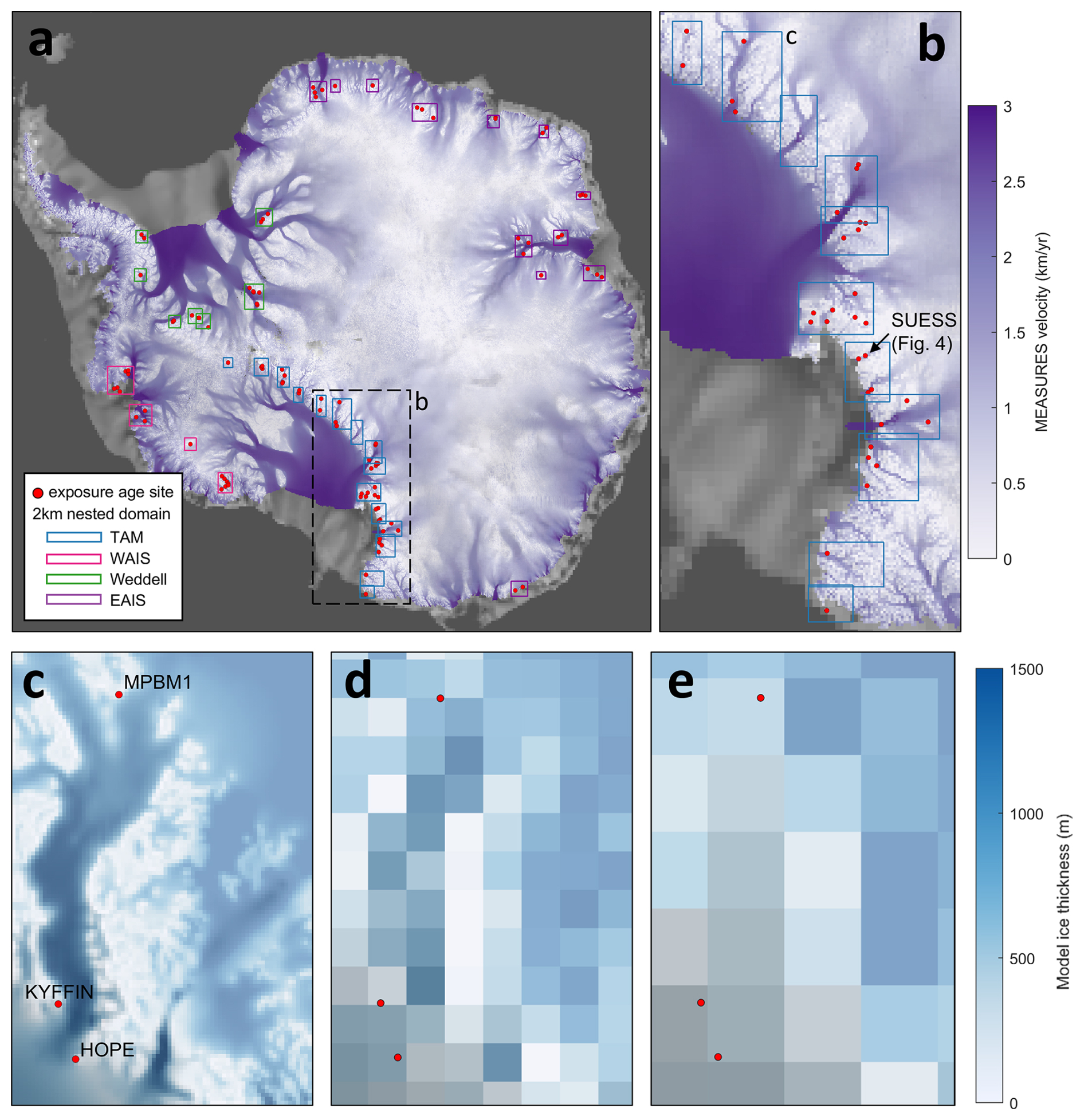
Figure 1 (a) Antarctic velocity map (MEaSUREs; Rignot et al., 2011) with locations of all exposure age sites from ICE-D (24 April 2024). 2 km nested domains are outlined, colored by region (TAM: Transantarctic Mountains; WAIS: West Antarctic Ice Sheet; Weddell: Weddell Sea region; EAIS: East Antarctic Ice Sheet margin). (b) Zoomed-in view to TAM region. (c) 2 km nested domain over Beardmore Glacier, showing higher-resolution features of the glacier trough. Exposure age sites located around the glacier are labeled according to the ICE-D site name (now showing only sites with > 3 youngest-bounding deglacial-age samples). The same domain is shown with a model grid resolution of 20 km (d) and 40 km (e).

2.4 Parameter variation

We generate a small ensemble of deglacial simulations to develop, implement, and analyze our model-data comparison framework. Thus, we focus on three key parameters, with the goal of producing a large spread in deglacial behavior in order to test the resolving power of our model-data comparison methodology (rather than represent the full parameter space). We vary “OCFACMULT”, a sub-ice oceanic melt coefficient, with values 1, 3, and 5 (non-dimensional; corresponds to K in Eq. (17) of Pollard and DeConto, 2012b). This parameter modifies the basal melt rate, which is a quadratic dependence of melt to ocean thermal forcing (Pollard and DeConto, 2012b). The model uses a spatially-varying basal sliding coefficient that is derived by inverting of modern ice velocities; a uniform value, “CSHELF” is applied to modern continental shelves. CHSELF provides a basal sliding coefficient value for regions outside of the modern inversion product (e.g., across the modern seafloor, where ice was grounded during the last glacial cycle, but is no longer present). Here we vary CSHELF from 10⁵, 10⁶, or 10⁷ (m yr⁻¹ Pa⁻², corresponds to C in Eq. 11 of Pollard and DeConto, 2012a). Finally, we vary “TLAPSEPRECIP”, which modifies the scaling of precipitation with temperature; because the model scales a modern climatology by a uniform temperature change through the last glacial cycle, the precipitation should also be scaled correspondingly. The PSU-ISM model employs a power-law relationship where TLAPSEPRECIP modifies this temperature shift to determine the spatial precipitation correction. Our standard value of TLAPSEPRECIP = 10 is analogous to the 7 % K⁻¹ best-fit Clausius-Clapyeron precipitation correction from Albrecht et al. (202b), and results in about 50 % less precipitation at the Last Glacial Maximum; here we also vary TLAPSEPRECIP to be 7 and 35 (corresponding to 2 and 10 % K⁻¹ Clausius-Clapyron rates, and about 20 % and 70 % drier at the Last Glacial Maximum, respectively; this brackets the range of deglacial precipitation changes that have been reconstructed from ice cores by Buizert et al., 2021, and also bounds the Clausius-Clapeyron parameter range explored by Albrecht et al., 2020b).

2.5 Preparing modeled deglaciation histories for data comparison

The ice sheet model accounts for bedrock glacial isostatic adjustment as the ice load distribution changes. Modeled bed elevation and thus ice surface elevation is influenced by these changes, so we extract only the ice thickness (ice surface elevation minus bed elevation) as the quantity to compare with geologic records of ice sheet thinning, following previous work (Briggs and Tarasov, 2013; Pollard et al., 2016; Lecavalier and Tarasov, 2025).

Computational and file-size constraints limit both the model grid size resolution as well as the time frequency that model output is captured. We conducted sensitivity testing to optimize these tradeoffs between model grid resolution and output frequency compared to improvements in capturing ice sheet behavior and the resulting differences in model scores. For nested domains over exposure age sites, the ice thickness field is written to the model output file every 500 years, and the extracted ice thickness curves are linearly interpolated down to a 20-year interval to more accurately identify a model age associated with a given elevation. The model ice thickness curve is isolated to thinning episodes only (in other words, data samples cannot be scored against time periods of model thickening; we assume that geologic deposits always reflect thinning, so only the parts of the model ice surface profile that follow an overall deglaciating trend are considered for model-data scoring). This methodology follows the original approach pioneered by Briggs and Tarasov (2013).

We incorporate a vertical window approach when evaluating the model ice thickness profile, to account for model resolution uncertainty (i.e., sub-grid elevation or thinning variability) and potential non-linear behavior in between model output write frequencies. Previous methodologies have varied approaches to address this issue: for example, Lecavalier and Tarasov (2025) account for modeled thickness change in neighbouring spatial grid cells – i.e., within a 120 km window spanning the exposure age site, also across a ± 500 year time window – in their error scoring method. Briggs and Tarasov (2013) calculate the ice thickness difference between different model resolutions in a modern gridded ice sheet product, with a maximum error of 100 m. Ely et al. (2019) similarly compare the model grid cell elevation and data sample elevation to account for a vertical downscaling uncertainty. Our approach most closely follows Pittard et al. (2022), who apply a blanket vertical tolerance of 250 m to each data point; this value was chosen because it represents a 5 % error on a possible 5000 m ice thickness maximum. Here we simply tailor the vertical error to directly reflect the deglacial ice thickness change at each site. Specifically, we calculate the model vertical window at each site as 10 % of the total modeled ice thickness change from LGM to present (for example, in our hypothetical model-data scoring scenario illustrated in Fig. 5, this vertical window is ± 47 m).

3 Exposure-age reconstruction of ice thinning at a site

In this section we describe a series of steps to access, prepare, and employ exposure age samples from across the continent to evaluate model-data fit. Cosmogenic nuclide measurements (Sect. 3.1) are first extracted from the inclusive and continuously updated ICE-D database (Sect. 3.2), and we develop an automated methodology to preprocess data (Sect. 3.3) and identify the subset of samples recording LGM-to-present deglaciation at a given site (Sect. 3.4). We recalculate sample uncertainties based on Monte Carlo iteration of the algorithm used to identify the post-LGM deglaciation history (Sect. 3.5), as well as explore the concept of a minimum “geologic” error at any given site (Sect. 3.6).

3.1 Measurement of cosmogenic nuclide concentrations

Cosmogenic nuclide measurements from clasts collected at a range of elevations across a nunatak site produce an age-elevation array in which clasts at higher elevations were uncovered first and therefore have older exposure ages. However, several added complications affect this basic relationship.

If a clast was derived not from the base of the ice sheet but from another nunatak where it was exposed previously, inheritance of cosmogenic nuclides produced during the first period of exposure would result in a spuriously old apparent deglaciation age. With the exception of a few sites where clasts are locally transported a short distance, this issue is fairly rare in Antarctica because 99 % of the continent is ice-covered. A much more common situation arises when clasts deposited on an ice-free area are repeatedly covered and uncovered by ice during multiple glacial-interglacial cycles. This is possible because in most locations in Antarctica, ice that covers rock outcrops during glacial periods is frozen to its bed and cannot transport or erode previously deposited material. Thus, many ice-free areas have not only fresh clasts that were first exposed during the most recent deglaciation (and therefore provide the correct age for this deglaciation), but also clasts that were originally emplaced during previous glacial terminations and have been covered and uncovered by ice several times. These multiply-exposed clasts have apparent exposure ages that overestimate the age of the most recent deglaciation. This is also true of bedrock surfaces, which typically display very old exposure ages integrating many periods of exposure. For this reason, bedrock surface exposure ages are not generally used to reconstruct LGM-to-present deglaciation. However, an exception to this is provided by measurements of cosmogenic ¹⁴C in rock surfaces; ¹⁴C has a half-life of 5730 years, so any ¹⁴C produced in previous interglaciations has been lost by decay and therefore ¹⁴C exposure ages on bedrock can be expected to accurately date the most recent deglaciation.

It is also possible for apparent exposure ages of clasts to be younger than the most recent deglaciation, typically because of postdepositional movement or overturning. Although this process is common in temperate environments, it is rare in Antarctica because the lack of liquid water and biota limits the possible processes that could cause postdepositional surface disturbance. Thus, it is likely that there exist more than zero exposure ages on Antarctic clasts that postdate the true deglaciation age due to postdepositional disturbance, but examples are expected to be very rare.

Thus, age-elevation arrays from Antarctic nunataks typically display both (i) exposure ages from “fresh” clasts that form a coherent array becoming older at higher elevation, and (ii) exposure ages from multiply-exposed clasts that are older than the most recent deglaciation.

3.2 The ICE-D exposure age database

This accessible online database contains all known Antarctic exposure-age data (including data published in peer-reviewed publications, and also unpublished data that have been made public due to public release requirements of funding agencies). The ICE-D database is designed to be inclusive (all exposure-age data known to have been collected from Antarctica are present in the database) but uncurated: although known measurement errors are corrected when discovered, all measurements that are believed to be accurate in the sense that the cosmogenic-nuclide concentrations were correctly measured and reported are included, and no effort is made to assess the degree to which exposure ages correctly date LGM-to-present deglaciation. ICE-D is continuously updated as new data are published; the dataset of exposure age measurements used here to develop our model-data comparison framework therefore include many new geochronological data that have not yet been systematically integrated into model reconstructions (for example: Rand et al., 2024; Suganuma et al., 2022 in East Antarctica; Stutz et al., 2023 in the Ross Sea region; Nichols et al., 2023 in the Amundsen Sea). Within the database, raw measurements are collated, and exposure ages are calculated with a consistent production rate scaling method so they are internally consistent (Balco, 2020).

3.3 Raw data preprocessing

Cosmogenic nuclide data are downloaded from ICE-D and preprocessed for model-data comparison. Unpublished sites are removed, along with sites located in the Antarctic Peninsula or sub-Antarctic islands. (We removed the Antarctic Peninsula sites in this study because the glacial dynamics in this highly mountainous and fjord-bisected peninsula region is difficult to meaningfully resolve in a continental-resolution simulation; however, all of the methodologies described here could be easily applied within that region as well.) The dataset is further constrained to LGM-age or younger samples. This preprocessing results in a preliminary dataset of 1276 cosmogenic nuclide measurements from 187 total sites (ICE-D dataset downloaded 11 May 2023).

We lump together sites that are located within the same model grid cell (combining them by sample elevation above the modern ice surface, rather than absolute elevation) in order to compare the model thinning history at a grid cell against all of the appropriate corresponding geologic information. This results in a smaller total number of “lumped sites” for model-data evaluation with the coarser-resolution 40 km continental domains compared to the 2 km nested domains. Subsequently, we refer to a “site” as a model-grid-cell-size area where exposure age data have been collected – i.e., a lumped site.

3.4 Identifying the youngest age/elevation samples at each site for model comparison

Cosmogenic nuclide measurements often result in a scatter of age measurements at the same elevation (for example, Fig. 2a) due to complications described above. Because inheritance issues lead to an old bias, the youngest-bounding age/elevation measurements are most likely to be robust. Therefore, in accordance with our goal of “non-curation”, i.e., eliminating any potential interpretation bias, we develop an automated methodology to identify the youngest age/elevation samples at a given site. This methodology connects a set of input samples with line segments, finding the path of greatest decrease in age in order to identify the youngest boundary in age/elevation space. The samples that are connected by these steepest-descent line segments thus reflect the youngest age/elevation measurements that can be interpreted to reconstruct ice thinning at a site. We apply this youngest-sample selection analysis following a Monte Carlo approach, randomly varying the age of each input sample within the measurement uncertainty range (Fig. 2b) and iterating 10 000 times to identify all potential “youngest” data points to use for our model/data comparison (Fig. 2c). We lump together different nuclide measurements in this youngest-sample selection analysis (i.e., treat them all equally) in accordance with our goal of “data agnosticism”. This procedure is applied only to sites with more than 3 samples that span more than 100m of elevation change, reducing the total number of sites to only those locations where a measurable pattern of significant deflation can be leveraged for model/data comparison (58 sites; 11 May 2023). Note that these 58 sites are further reduced to 50 (44) locations for evaluating 2 km (40 km) model simulations because sites that fall into the same model grid cell are lumped together, as described above.

This automated method for identifying the youngest age/elevation samples to use for model-data comparison aims to replace the manual step of “expert interpretation” that is required for converting exposure age measurements into a curated geologic constraint, e.g., as in Lecavalier et al. (2023). While this automated approach will identify the “true” youngest age/elevation space for most sites, there are edge cases in which this method may fail; namely, (i) rare postdepositionally-disturbed ages, (ii) a case where all or nearly all samples have inheritance, so the youngest age-elevation bounding samples are not statistically identifiable from the surrounding “noise”, and (iii) data with analytical errors. We note that although some of these “edge cases” may be caught by manual curation (most likely iii), many would not. Our approach accepts that some fraction of the constraint data set is spurious, and we therefore prevent a single pathological site from dominating the model score; see Sect. 4.2.4.

Figure 2 (a) Sample illustrative dataset of cosmogenic nuclide measurements collected along an elevation transect, with error bars denoting measurement error. (b) One iteration of our youngest-sample identification scheme (identifying the youngest age/elevation bounding range given randomly varied age/elevation data points within measurement uncertainty). (c) 10 000 Monte Carlo (MC) iterations produce a range of youngest-boundary age/elevation trajectories, and identify all possible youngest data points (green) to use for model/data comparison. Data points shown in orange in (c) are never part of a possible deglaciation trajectory and are therefore considered to be the result of nuclide inheritance and discarded (i.e., not shown in d). (d) Red dashed lines show the 1σ standard deviation of the Monte Carlo youngest age/elevation space; this width (the 1σ range at a given elevation, including a 20 m vertical tolerance range) determines the uncertainty for each data point (red error bar).

3.5 Measurement precision and sample age uncertainty

While each sample has a reported measurement error that is derived from the analytical uncertainty on the nuclide concentration measurement, a number of datasets in which multiple exposure ages are measured at the same elevation show that the measurement errors of each sample are typically smaller than the range of sampled ages at a given elevation (as one example, see Mt. Hope (HOPE) in Spector et al., 2017). In other words, the uncertainty associated with a cosmogenic nuclide measurement is two-fold: the measurement precision error (established through repeat measurements in a laboratory), and the geologic uncertainty (i.e., the spread in ages that would result from repeated sampling at a given elevation at the field site). In general, geologic uncertainty arises because nunataks are not smooth surfaces emerging from a perfectly flat ice surface; both the bed topography and the ice surface topography are variable, so all locations at the same elevation do not deglaciate at exactly the same time. We incorporate both sources of error within our misfit calculations by identifying the age range across the Monte Carlo “cloud” at any given elevation (the 1σ range) to use as the uncertainty associated with each sample (Fig. 2d). We assess Monte-Carlo-derived uncertainties only when a site has more than 3 samples (otherwise, the measurement error is used). This approach considers both the measurement precision error (which is encompassed by the Monte Carlo random variation of sample age within measurement uncertainty) as well as the uncertainty associated with the spread in data points.

Although we consider only age misfits in our model data evaluation framework, we indirectly account for elevation uncertainty here by applying a vertical tolerance range when identifying the Monte-Carlo-derived uncertainty. For each data point, we find the associated Monte Carlo uncertainty by calculating the greatest difference between the ± 1σ MC curves within a 20-meter-high vertical tolerance range. This approach weights misfit calculations to prioritize samples where glacial deflation is occurring; within a vertical tolerance range, uncertainties are greater for samples where the recorded ice surface elevation change is minimal (for example, Fig. 2d samples from ∼ 15–10 ka), which reduces the misfit for these samples compared to samples that record rapid thinning.

3.6 Calculating a minimum geologic error

The ideal site for reconstructing ice sheet thinning has dense samples collected at a range of elevations. At these well-sampled sites, repeated sampling at an elevation often reveals a wider range of uncertainty than the measurement error (geologic uncertainty, as discussed above in Sect. 3.5). Sites with only a few samples, however, can misleadingly appear to have much smaller geologic uncertainties since there are inherently fewer conflicting data points. We therefore identify a “minimum geologic error” reflecting the geologic uncertainty associated with repeated sampling across a site.

We identify a uniform minimum geologic error of 495 years, based on the 95th percentile of all Monte-Carlo-derived sample uncertainties from all sites. Figure 3 shows that a large number of samples have much lower uncertainties – these tend to be from sites with just a few samples, with misleadingly low uncertainty derived from the Monte-Carlo youngest-age-elevation-boundary algorithm. There is also a significant fraction of locations where this uncertainty is around 500 years, but uncertainties tail off after this value (larger uncertainties tend to reflect larger measurement precision errors that drive up the Monte-Carlo-derived errors). Thus, we interpret this value to reflect the smallest reasonable uncertainty we could produce at a site with a large number of samples. This `minimum geologic error' provides a lower bound for the uncertainty for each sample when calculating misfit (e.g., σ_samp in Eq. 3). This is intended to level the playing field between sites with multiple widely distributed samples and sites with only a few (or clustered) samples.

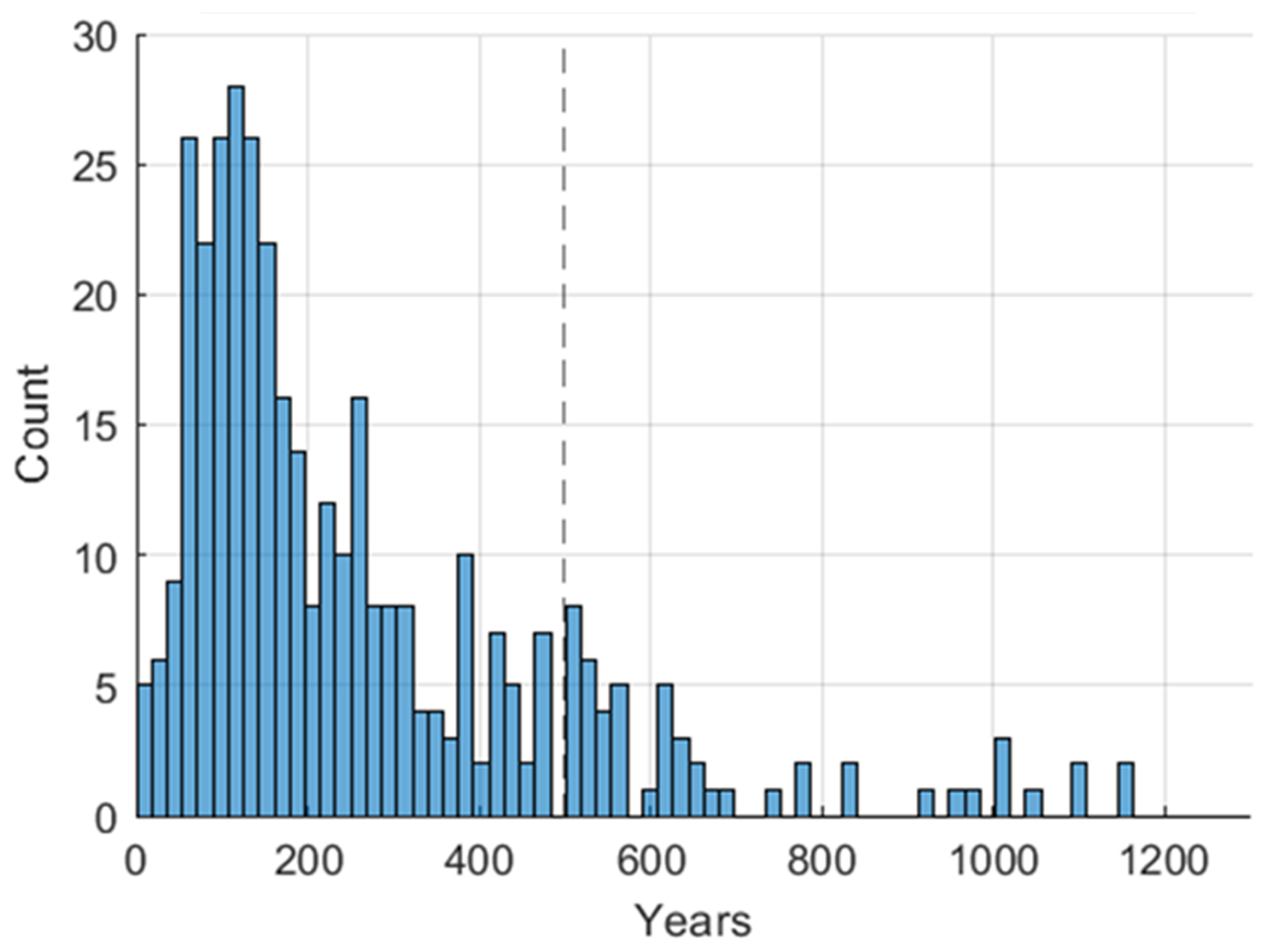
Figure 3 Calculated error for each age/elevation data point across all sites (using the Monte-Carlo-derived youngest age/elevation scheme described above). The “minimum geologic uncertainty” we identified is 495 years (dotted line).

4 Description of model-data comparison techniques

Model resolution presents a challenge for aligning modeled and observed thinning at a site: specifically, that there is no feasible model resolution that will exactly capture all small-scale topography of rock and ice at an ice margin retreating through mountainous terrain. Thus, key quantities that could be compared across models and data – namely, the absolute ice surface elevation, or the absolute magnitude of thickness change – are not necessarily expected to exactly match between models and reality. However, the timing of thinning and the variation in thinning rates through time should not be strongly subject to these issues. We therefore develop two methods to align modelled and measured thinning profiles, that focus on these more robust features of model-data fit (Sect. 4.1). We describe our formulation of model-data misfit and introduce two corresponding metrics for model-data assessment (Sect. 4.2). The “float scoring” approach evaluates ice thickness change unregistered to a vertical datum, allowing the modeled ice history to float vertically to minimize model-data misfit at a site. We also identify a “best time offset” value, the horizontal time adjustment that minimizes site misfit, to specifically isolate timing differences between modeled and measured ice thinning histories. These metrics are applied at every exposure age site with multiple (> 3) samples. Model scores are derived by averaging site misfits across the continent and applying a site-by-site spatial weight based on data density.

In addition to model-data fit with respect to ice thinning patterns at a site, we also investigate model-data fit with respect to the maximum amount of ice sheet thinning during the last deglaciation (i.e., LGM ice surface relative to modern ice surface) in Sect. 4.3. Specifically, we identify a separate dataset of exposure-age sites where a maximum ice thickness change can be estimated from the geologic record. Any exceedance of the modeled maximum thinning at these locations is averaged across the continent (and weighted with respect to the reliability of the geologic constraint); the resulting “ice thickness exceedance” model score provides another metric for evaluating model-data consistency. Table 1 provides a summary of terms for each of our three unique model-data misfit metrics.

These individual metrics are designed to stand alone; each approach addresses different questions about model-data fit, and thus we do not combine these metrics together into one total model score because the optimal weights for combining these various metrics would differ based on the user's interest and motivating question.

Table 1 Description of terms and misfits.

n/a: not applicable.

4.1 Finding quantities in common: aligning modeled and measured ice thinning reconstructions at a site

Here we develop several strategies that attempt to fairly compare modeled and observed thinning, in response to two main categories of obstacles: first, model representation of the correct glacial setting; and second, vertically aligning models and data with respect to an elevation datum.

4.1.1 Model-data alignment with respect to glacial setting

While our high-resolution (2 km) nested simulations are now able to capture most glacier trunks (Fig. 1c), this increased spatial granularity can introduce a mismatch between the glacier thinning that is recorded at an exposure age site and model behavior at the precise sample locations. This mismatch occurs because cosmogenic nuclide measurements at a site are collected along an elevation transect; the progressive exposure of bedrock along this transect is used to infer the surface lowering of an adjacent glacier or ice mass. However, especially at high grid resolutions, the modeled ice thickness history corresponding to the precise sample location(s) does not always capture the full thinning behavior of the adjacent glacier. For example, mountain-side grid cells cease recording glacial deflation once the grid cell becomes ice-free, although ice sheet deflation continues in the adjacent glacial valley.

To identify the model grid cell capturing a comparable quantity to exposure age data reconstructions, we develop an automated methodology for identifying the nearest glacier grid cell (rather than using the precise lat/lon of the site samples to extract a model thinning history). We apply this methodology only for the 2 km resolution nested domains, where glacier valleys and adjacent topographic highs are resolved. Specifically, we identify the nearest adjacent glacier grid cell based on average velocity throughout the simulation. This automated methodology selects the location with maximum velocity within a 4×4-grid-cell (8 km) search radius around the mean site lat/lon (the average location across all samples in the site). This search radius was chosen in order to encompass the spatial spread of individual sample locations for most sites; in other words, to properly reflect the thinning history at a site, the search radius should cover the entire hillside where an elevation transect of samples were collected, and our model/data comparison approach should use a thinning history from the grid cell at the base of that hillside transect of samples.

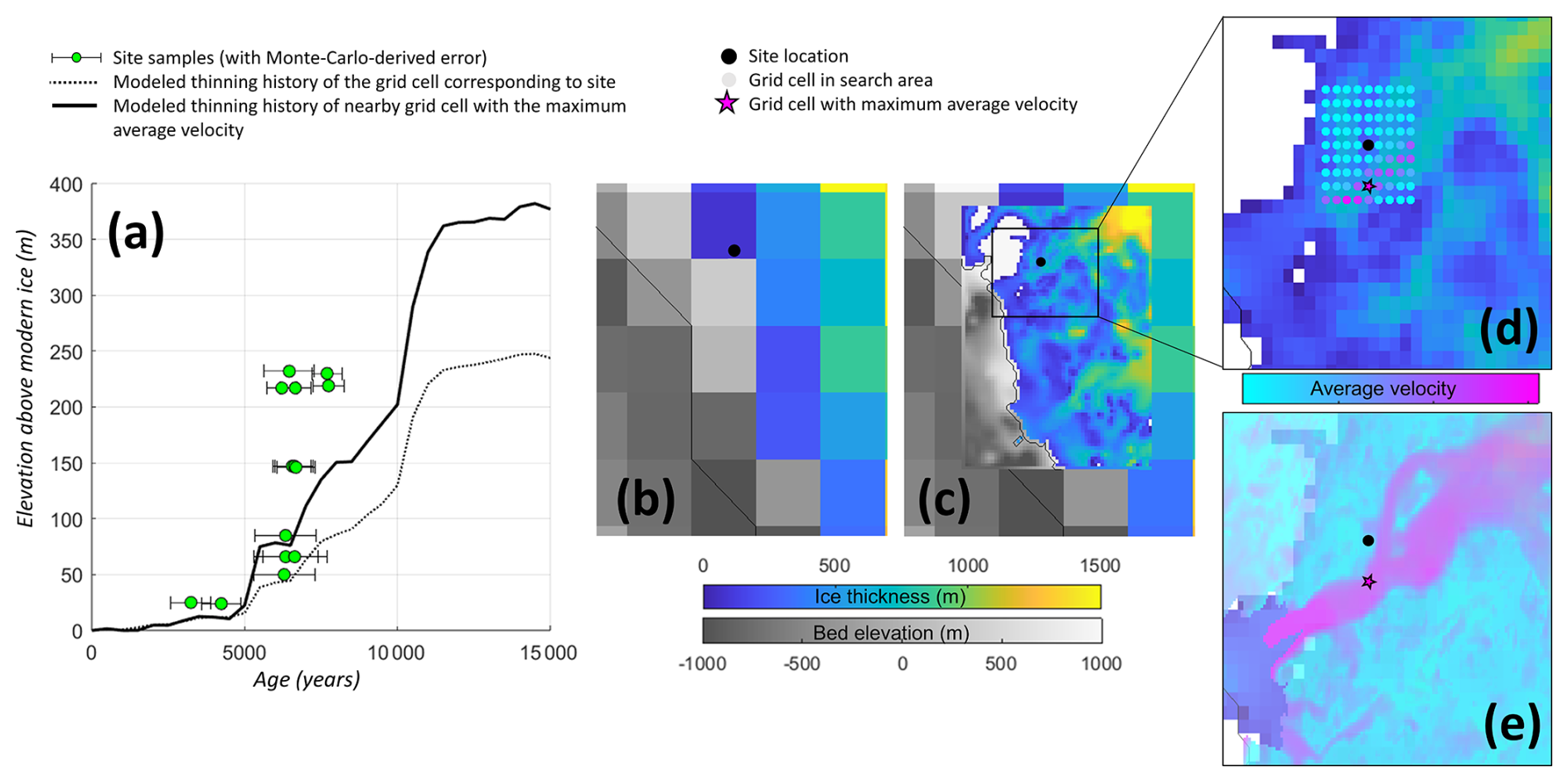
Figure 4 Model-data alignment at SUESS site, located along the Transantarctic Mountains (Mackay Glacier, Mt. Suess; location shown in Fig. 1). (a) Exposure age record of thinning (green dots; original data from Jones et al., 2015) compared to modeled thinning from the 2 km nested domain (dashed black line shows thinning at the grid cell corresponding to the actual sample location; thick solid black line shows thinning at the nearby grid cell with maximum velocity). (b) Site location in a 20 km (intermediate-resolution) model compared to (c) the 2 km nested domain. (b, c, d) The black dot shows the mean location of the site (averaged across all samples at the site). (d) This approach searches for the location of maximum velocity near the site. Dot color shows the average velocity of each grid cell within the search area throughout the run. The black star denotes the location with maximum velocity, which occurs in the adjacent glacier trough; the thinning history at this location is used for model/data comparison. (e) Modern velocity from the MEaSUREs dataset (Rignot et al., 2011) superimposed over the modern model ice thickness for this nested domain.

For our continental (coarser resolution) simulations, we extract modeled thinning history from the grid cell exactly corresponding to the precise sample lat/lon location. If the transect of samples comprising a single site spans different model grid cells, we use the model thickness history corresponding to each sample.

4.1.2 Model-data alignment with respect to a common ice surface baseline

Vertically aligning modeled and measured ice surface elevations at a given site requires a common elevation datum. Comparing the absolute ice surface elevation change between modeled and measured ice sheet reconstructions (even when these quantities are capturing the same glacial setting) is challenging because topography and ice flow vary at spatial scales that are smaller than model grid cells (for example, Fig. 4). Thus, except perhaps in the rare case of an isolated nunatak emerging from a flat interior region of the ice sheet, the ice surface elevation in a model grid cell is unlikely to be exactly the same as the true ice surface elevation at any specific location within that grid cell. In fact, true ice surface elevation variability within a large grid cell in mountainous topography may be much larger than the magnitude of LGM-to-present thinning. This issue is commonly dealt with in model-data comparison endeavors by assuming that while the model does not accurately predict the true ice surface elevation at an exposure-dating site, the rate, timing, and amount of ice thickness change should be similar between model and data. That is, models and data are compared on the basis of thickness change relative to present (registered to the modern ice surface) and not on the basis of absolute surface elevation; all previous model-data comparison efforts (Briggs and Tarasov, 2013; Pollard et al., 2016; Pittard et al., 2022; Lecavalier and Tarasov., 2025) have accordingly aligned modeled and measured thinning profiles with respect to ice thickness above modern. However, identifying a modern ice surface elevation that is common to both models and data is often not straightforward. The true ice surface elevation at a mountainous exposure age site, already highly variable due to topography, is further complicated by local factors such as snow buildup patterns like wind scoops and blue ice areas (e.g., Bintanja, 1999), and ice flow perturbations caused by the nunatak itself (e.g., Mas e Braga et al., 2021). The modeled ice surface elevation is also not always reliable, since (a) many nunatak features are smaller than even the high-resolution 2 km nested model domains, and (b) the model ice sheet configuration in the last timestep (“modern”) will not perfectly reflect the true modern ice sheet configuration. Furthermore, the “modern” ice-sheet state is a rapidly shifting baseline; many sites have deflating ice thicknesses on decadal timescales, and models tend to produce WAIS collapse under modern climatological forcings.

Due to these issues with aligning the modern baseline, neither the absolute ice surface elevation nor the absolute magnitude of thickness changes are necessarily expected to quantitatively match between models and reality. However, the timing of thinning and the spatiotemporal variation in thinning rates are mostly independent of these resolution and alignment issues; we therefore develop two metrics that isolate these deglacial thinning characteristics that can be more robustly compared across models and data (the float scoring metric and best-time-offset metric, described quantitatively in Sect. 4.2.2 below).

4.2 Quantifying model-data misfit

4.2.1 Site misfit calculation

Model-data misfit at a data sample (m_samp) is calculated from the time gap (Δt) between modeled and measured ice thinning histories, relative to the sample uncertainty (σ_samp), as illustrated in Fig. 5. The sample misfit m_samp is then provided as a mean squared error:

$$\begin{array}{}\text{(1)}& m_{\mathrm{samp}}={\left({\displaystyle \frac{\mathrm{\Delta }t}{{\mathit{\sigma }}_{\mathrm{samp}}}}\right)}^{\mathrm{2}}\end{array}$$

This time gap Δt is defined as the difference between D_model, the time that the model reaches the elevation of the sample, and D_samp, the closest time of exposure of the data point (i.e., within the sample age uncertainty). Because we apply a vertical elevation window approach when evaluating the model ice thickness profile (chosen here to be 10 % of the total modeled ice thickness change from LGM to present), Δt is set as the smallest time gap within this vertical elevation window (described in Eq. 2 and graphically illustrated in Fig. 5 inset). Sample uncertainty is either subtracted or added, to produce the smallest Δt.

$$\begin{array}{}\text{(2)}& \mathrm{\Delta }t=\left\{\begin{array}{ll}\left(D_{\mathrm{model}}-[D_{\mathrm{samp}}\pm {\mathit{\sigma }}_{\mathrm{samp}}]\right)& \text{if model and data}\\ & \text{elevations intersect}\\ \left(D_{\mathrm{samp}}-{\mathit{\sigma }}_{\mathrm{samp}}\right)& \text{if model never thins }\\ & \text{to data elevation},\\ & D_{\mathrm{model}}=\mathrm{0}\\ \mathrm{\Delta }{t}_{\mathrm{u}}& \text{if model never}\\ & \text{thickens to data}\\ & \text{elevation}\end{array}\right.\end{array}$$

Δt_u is a uniform time gap, designed to impose a misfit penalty if the modeled ice thickness range fails to encompass the observed range (see “Scoring samples outside of the range of model ice thickness change” below).

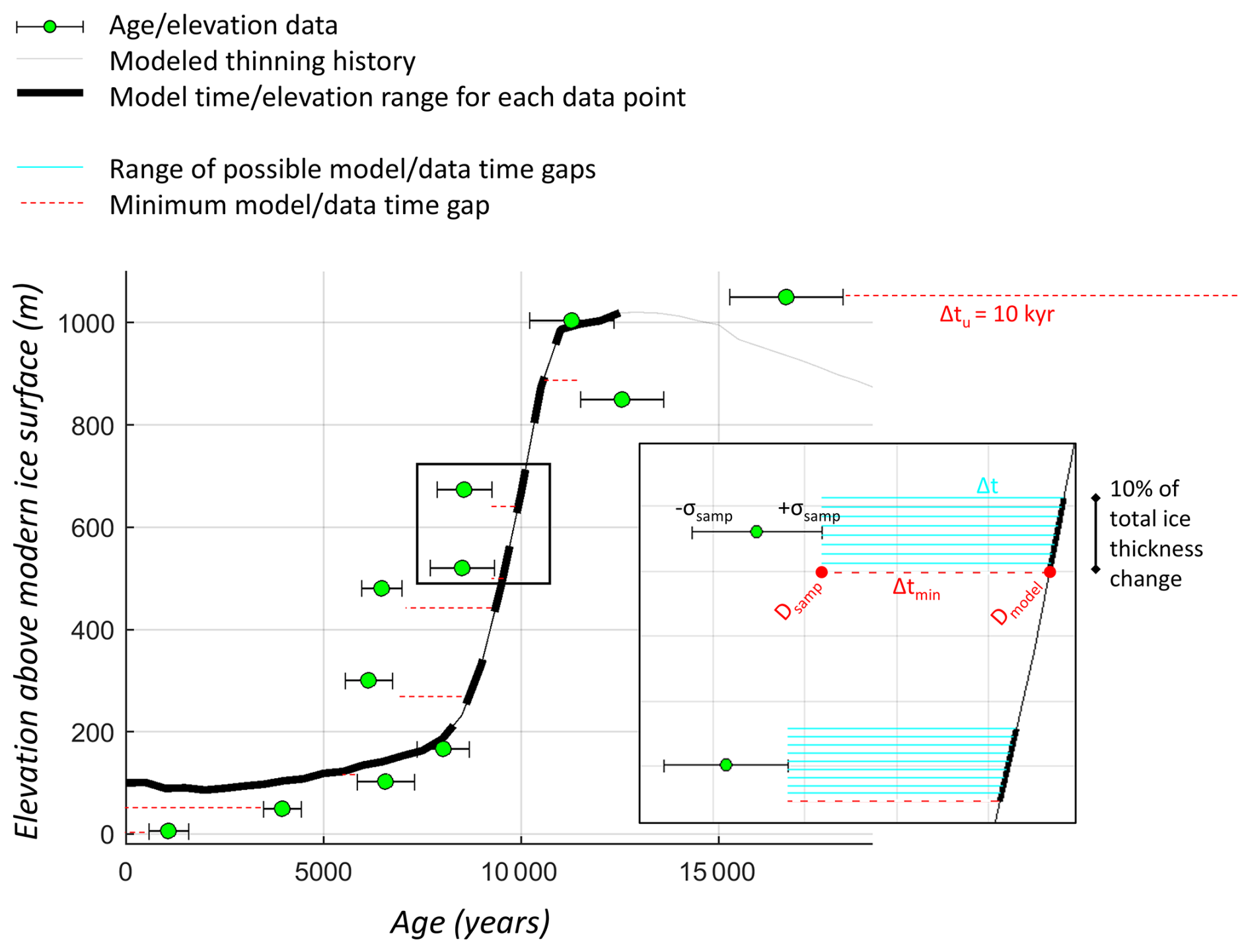
Figure 5 Graphical illustration of model/data misfit components (exposure age samples compared to a “floating” ice thickness history). The thicker lines denote the model vertical window (elevation range for assessing model thickness history against each data sample). The model vertical window is defined as 10 % of LGM-to-present ice thickness change; in this case, ± 47 m. Δt, the smallest time gap for each sample, is identified with a red dashed line.

Sample age uncertainty σ_samp is derived from the 1σ width of the Monte Carlo spread in possible youngest age/elevation thinning histories at each site (Sect. 3.5). The sample uncertainty σ_samp is then constrained by the minimum geologic uncertainty of 495 years (Sect. 3.6).

$$\begin{array}{}\text{(3)}& {\mathit{\sigma }}_{\mathrm{samp}}=max\left({\mathit{\sigma }}_{\mathrm{samp}\mathrm{\_}\mathrm{MC}},\mathrm{495}\right)\end{array}$$

The site misfit m_site is calculated as the average of all (n) sample misfits at a site:

$$\begin{array}{}\text{(4)}& m_{\mathrm{site}}={\displaystyle \frac{\mathrm{1}}{n}}\left(m_{\mathrm{samp}\mathrm{1}}+m_{\mathrm{samp}\mathrm{2}}+\mathrm{\dots }{m}_{\mathrm{samp}n}\right)\end{array}$$

Note that we assess model performance only with respect to time – in other words, misfits are simply the squared error of the time gap between an exposure age at a given elevation and the time that a modeled ice sheet simulation deflates to that thickness above present. Although some earlier literature similarly isolated age misfits (e.g., Ely et al., 2019), preceding comprehensive model-data comparison efforts considered both time and elevation of the ice thickness profile (i.e., sample misfit is calculated based on the time gap as well as the vertical elevation gap; e.g., Briggs and Tarasov, 2013; Pollard et al., 2016). The decision to consider only the time misfit is determined by (i) the fact that exact matches between model and actual ice surface elevations and ice thickness changes are unlikely, due to model resolution limitations as discussed above (even 2 km model grid cells are much larger than spatial variations in ice and rock topography surrounding many sample locations); and (ii) the related observation that models are much more likely to correctly represent the large-scale timing of variations in the ice thinning rate than the exact ice surface elevation at a particular site. This reasoning leads to our strategy of varying the absolute ice thickness change as a nuisance parameter in our “float scoring” metric described above. Nevertheless, our approach indirectly evaluates model ice thickness changes against reality by attempting to match the shape, even if not the absolute elevation, of the thinning curve (e.g., Fig. 6). In addition, the misfit penalty applied when the model thinning history fails to span the magnitude of the actual thinning history recorded at a site (see discussion below) is an indirect assessment of the model performance with respect to observed thickness change.

4.2.2 Metrics for model-data scoring

Float scoring metric (ice thickness change unregistered to a datum). This approach allows the modeled ice history to “float” vertically, by applying a vertical adjustment to modeled ice elevations to minimize site misfit (Table 1). This isolates the model fit to the reconstructed timing and amount of ice sheet thinning. If model thinning occurs at the same amount/same rate/same time as the exposure age dataset, the vertical offset will produce a good misfit. But if model thinning happens at the wrong time, or too slowly, or not enough, this approach will produce a bad misfit even with the best-fit elevation shift (Fig. 6). The “float scoring” metric is applied to sites with > 3 samples (with Monte-Carlo-derived uncertainties) and > 100 m of elevation change recorded at the site (n=49, with 2 km grid resolution lumping, 24 April 2024).

Figure 6 Comparing measured and modeled ice thinning using a best-fit vertical adjustment, using the hypothetical exposure age samples from Fig. 2. Model ice thickness histories are systematically shifted up and down in elevation; the best-fit model profile (cyan) is used to calculate site misfit. The model simulation in (a) produces a good fit to the ice thinning recorded by cosmogenic nuclide samples, while the model in (b) is not able to replicate the timing and amount of measured ice thinning regardless of vertical adjustment.

Best-time-offset metric. Here, a range of time offsets are applied to the model thinning curve at each site, to identify the best-fit time offset (in kyr) that minimizes site misfit (Fig. 7). Specifically, this time-offset analysis is applied to the best-fitting “float” curve obtained via the float scoring approach described above. The resulting best-time-offset metric can be used to assess how well a model represents the timing of ice sheet thinning, and can also potentially provide insights on systematic issues with model forcing datasets. For example, a model run that systematically under- or overestimates the timing of ice sheet change across a specific region or even the entire ice sheet might indicate some persistent offset issue in the atmospheric or ocean climatology model forcings. On the other hand, if model-data offsets are randomly (rather than systematically) distributed among sites in close proximity, this could motivate a reassessment of potential issues with either model resolution or the interpretation of geologic data.

In addition to isolating the model fit to the recorded timing of deglaciation, the best-time-offset analysis can also be used to identify the “minimized” site misfit (the “site best-time-offset misfit”) that eliminates any timing mismatches and reflects only the model-data fit with respect to the shape of the thinning curve. In other words, we can isolate just the rate and pattern of thinning by identifying this best possible misfit at a site (i.e., the minimized site misfit after applying both the best-fit vertical elevation shift as well as the best-time-offset horizontal shift to a model thinning curve). This approach allows us to evaluate model ability to replicate the overall style of deglaciation as recorded by exposure age data, independent of any potential time lag between models and data.

Figure 7 Calculating a best-time-offset value at a site. (a) Exposure age samples and model ice thickness profile (dashed black line) from Fig. 6. The model thickness profile is systematically shifted earlier and later via an imposed “time offset”; time-offset model thickness profiles are colored by the resulting site misfit. The model thinning curve with the best-time-offset value (2 kyr) is shown with a dashed red line. This −2 kyr time-offset model thinning curve results in the minimum site misfit (the “site best-time-offset misfit”). This process is demonstrated graphically in (b), where the original model thickness profile (offset = 0) is shown as a black dot, and the best-time-offset model profile is a red dot.

4.2.3 Scoring misfits for samples outside of the range of model ice thickness change

At some sites, the observed amplitude of deglacial thinning exceeds the range of LGM-to-present ice-sheet deflation simulated by a model at the site location. Samples collected at higher elevations than simulated by a model thus lack a corresponding modeled age to use for determining the sample misfit. In this case, we prescribe a uniform time-gap (Δt_u; Eq. 2; Fig. 5). The absolute value of this imposed time-gap influences the misfit calculations; a relatively large time-gap (e.g., 20 kyr) would amplify site misfits where model thinning is underestimated, heavily penalizing model simulations with suppressed deflation patterns, while a relatively small time-gap (e.g., 5 kyr) would produce model scores that are less influenced by sites where modeled ice thickness change does not exceed the measured thinning amplitude. Our model-data scoring approach here is designed to identify model simulations that reproduce not only the amplitude of deglacial ice thickness change, but also the timing and rate; we therefore select a uniform time gap Δt_u=10 kyr, which inflates misfits for sites where model thinning amount is underestimated but does not over-amplify this particular type of model-data mismatch to dominate the model score.

When we allow the model ice thickness curve to `float' vertically (to find a minimized site misfit), exposure age samples collected from near the present ice margin can be located below the adjusted model thickness curve. To assess a misfit for these samples, a corresponding model age of deglaciation is required; since the model never thins to the data elevation, we impose a modern age of model deglaciation (i.e., D_model=0; Eq (2), Fig. 5). This reflects the need for the model to continue to thin into the future in order to reach the sample elevation.

4.2.4 Synthesizing site misfits into a model score

Capping site misfits. When modeled ice thickness patterns are drastically different from the measured thinning history, extremely large site misfits can be produced. These outliers with significantly large site misfits often dominate the overall model score, which we consider to be a disproportionate and undesirable impact. In this framework, model scores should reflect the cumulative model “fit” to all sites: a model simulation should score lower (better) if it reproduces ice thinning at most sites satisfactorily but completely misses a few sites, compared to a simulation that reproduces thinning measurements poorly across the continent but has a marginally better misfit at outlier site(s). We therefore implement an upper limit on site misfits, to reduce the impact of outliers on the overall model score and reflect more meaningful model improvements that incrementally reduce misfits at the majority of sites. Here we deploy site misfit ceilings (e.g., upper bounds) by empirically determining a maximum information-bearing site misfit – below this value, a lower-scoring model simulation does reflect a physically realistic improvement in model representation, but at higher (worse) values, a smaller site misfit does not reflect meaningful improvement in model representation of the data (and thus does not have resolving power and should not impact the total model simulation score). An example is shown below in Fig. 8. We therefore establish a site misfit cap (m_max=50, in Eq. 5) for the float scoring metric.

Figure 8 Site float misfits at KRING (David Glacier, Mt. Kring) for various model ensemble members (from top to bottom: 7–0.3–35, 7–2–35, 5–5–35, 5–5–10, 5–2–10). Below m_max=50, lower (better) site float misfits indicate a physically realistic improvement in model representation. Above this misfit cap, a lower misfit does not reflect meaningful improvement in model representation of the data. Original exposure-age data from Stutz et al. (2021).

Spatial weighting. We apply a spatial weight S_w to each site to avoid biasing model scores towards well-sampled regions. Site misfits are inversely weighted based on the number of regional sites (Fig. 9). The number of regional sites are identified at each site location within a region size of 10° longitude by 5° latitude (cf. Briggs and Tarasov, 2013; approximately the characteristic scale of viscoelastic response). S_w is calculated by normalizing the number of regional sites around each site location, and taking the inverse, to provide a spatial weight. Our approach deviates from the inter-data-type weighting scheme of Briggs and Tarasov (2013) in that we use the number of regional sites rather than the number of regional data-points (samples) to establish our spatial weights; here we aim to treat every site as equally robust.

Figure 9 Spatial weights at each exposure age site used for scoring (i.e., with more than 3 samples that span more than 100 m of elevation change). Sites are inversely weighted based on the number of nearby sites.

Each model simulation score (M_model) is calculated by taking the mean of all site misfits (n) across the continent after multiplying each site misfit m_site by the spatial weight S_w:

$$\begin{array}{}\text{(5)}& M_{\mathrm{model}}={\displaystyle \frac{\mathrm{1}}{n}}{\sum }_{i=\mathrm{1}}^n\mathrm{mean}(m_{\mathrm{site},i},m_{\max })\cdot S_{\mathrm{w},i}\end{array}$$

4.3 Maximum ice thicknesses: geologic constraints and model exceedances

Here we isolate and evaluate the amplitude of ice sheet deflation as an additional measure of model/data fit. To complement our primary dataset of continent-wide deglacial exposure ages, we compile an additional dataset of last-glacial-cycle maximum ice thickness constraints at sites where the local LGM ice thickness change can be estimated, and correspondingly develop an independent model-data metric to evaluate the modeled amplitude of ice thickness changes.

This metric complements the scoring approaches described above, which do not explicitly penalize vertical misfits (i.e., model thinning amplitudes that are drastically larger than the amplitude of thinning recorded by terrestrial data). We treat this particular challenge as a separate scoring metric because of several characteristics of the exposure-age data that make it difficult to estimate the total LGM-to-present ice thickness change at most sites. First, many exposure-age data sets are collected from nunataks whose exposed height is shorter than the ice thickness change at the LGM (for example, LONEWOLF1 site (Byrd Glacier, Lonewolf Nuntataks, LW1 Nunatak; data collected by Stutz et al., 2023, and shown below in Sect. 6.2). They only became uncovered, and capable of recording ice thinning, partway through deglaciation, so data sets from these sites typically have a highest observed exposure age sometime within the Holocene, when deglaciation is expected to have been well under way. Sites of this type provide a lower limit on LGM ice thickness change (because the ice must have been thicker than the highest postglacial erratic), but no upper limit. Nunataks that are tall enough to have remained exposed at the LGM, on the other hand, typically display a LGM-to-Holocene array of exposure ages up to the LGM ice thickness, with only ages older than the LGM (commonly much older by hundreds of thousands of years) above this elevation (for example, at QZH (Reedy Glacier, Quartz Hills; Todd et al., 2010). We use this diagnostic pattern to identify sites that constrain the LGM ice thickness. However, this relationship is never completely unambiguous because of sampling bias; there is no way to completely disprove the hypothesis that the LGM ice surface elevation was higher but no post-LGM erratics were collected at that elevation. Thus, it is likely that there are some sites where the diagnostic feature that is identified here – pre-LGM ages above a LGM-to-Holocene age array – is misleading.

We also exploit another feature of the exposure-age data set to identify LGM ice thickness constraints: cosmogenic carbon-14 exposure ages, which are a minority of the total exposure-age data set but exist at a number of sites. Where ¹⁴C data exist, a boundary between below-steady-state and at-steady-state ¹⁴C concentrations is unambiguously diagnostic of the LGM ice thickness (Balco et al., 2019; Goehring et al., 2019; Nichols, 2023; see Sect. 3.1 for more information).

We note that LGM moraines with unambiguous weathering contrasts could also be used as LGM ice thickness constraints to complement the exposure-age data. However, we have not attempted to quality-control and compile these observations here, due to difficulties in distinguishing LGM from pre-LGM moraines based on appearance alone (Balco et al., 2016; Bentley et al., 2017), and ambiguous interpretations of weathering contrasts (i.e., as an LGM ice limit or a subglacial thermal boundaries below the ice surface; Sugden et al., 2005).

4.3.1 Identifying maximum ice elevation from a transect of exposure ages at a site

We construct a dataset of LGM maximum ice thickness constraints using two cosmogenic-nuclide-based indicators that can be recognized by simple data-processing algorithms: (1) steady-state ¹⁴C measurements that preclude LGM ice cover above a specific elevation; and (2) transitions between lower-elevation measurements of post-LGM exposure ages and higher-elevation measurements of extremely old ages (i.e., samples that significantly predate the LGM). These elevation constraints are then translated into a maximum ice thickness limit (based on the modern ice surface elevation) to compare with model output. For the present data set, we identify 3 sites where steady-state ¹⁴C concentrations provide a maximum LGM ice thickness constraint, and 29 sites where measurements reveal a transition between post-LGM and pre-LGM ages, resulting in an LGM thickness constraint dataset of 32 sites. (Data were extracted from ICE-D and analyzed on 14 March 2024, see Code and Data Availability statement)

To obtain a maximum thickness constraint from ¹⁴C data, we identify sites that have at least one sample with a ¹⁴C concentration at or above the steady-state value that was collected at a higher elevation than at least one sample with a concentration below the steady-state value. We therefore assume that measurements at this site span across the maximum LGM ice elevation. ¹⁴C saturation marks samples that remained uncovered by ice throughout the last glacial cycle; we therefore interpret the minimum elevation of saturated ¹⁴C samples to be a maximum elevation limit of the ice sheet at that site.

When no steady-state ¹⁴C concentrations are observed at a site, we identify LGM ice thickness constraints by recognizing the characteristic pattern of a cluster of very old (pre-LGM) ages at higher elevations, and a record of post-LGM ice thinning at lower elevations (an example is shown in Fig. 10). We first require that the site includes more than one pre-LGM age sample that is located higher than all of the post-LGM ages. We then calculate the average youngest age-elevation boundary for all samples (following the same Monte Carlo procedure as in Sect. 3.4) to identify the elevation at which this youngest age-elevation boundary intersects the LGM (conservatively defined here as 30 ka). We interpret this intersection elevation as a minimum estimate of the LGM limit (rather than the highest post-LGM-age sample, since it is unlikely that the highest young erratic is the true LGM limit). Finally, we identify the next-highest sample above this intersection elevation where old (pre-LGM) ages are measured, as a constraint on the maximum thickness.

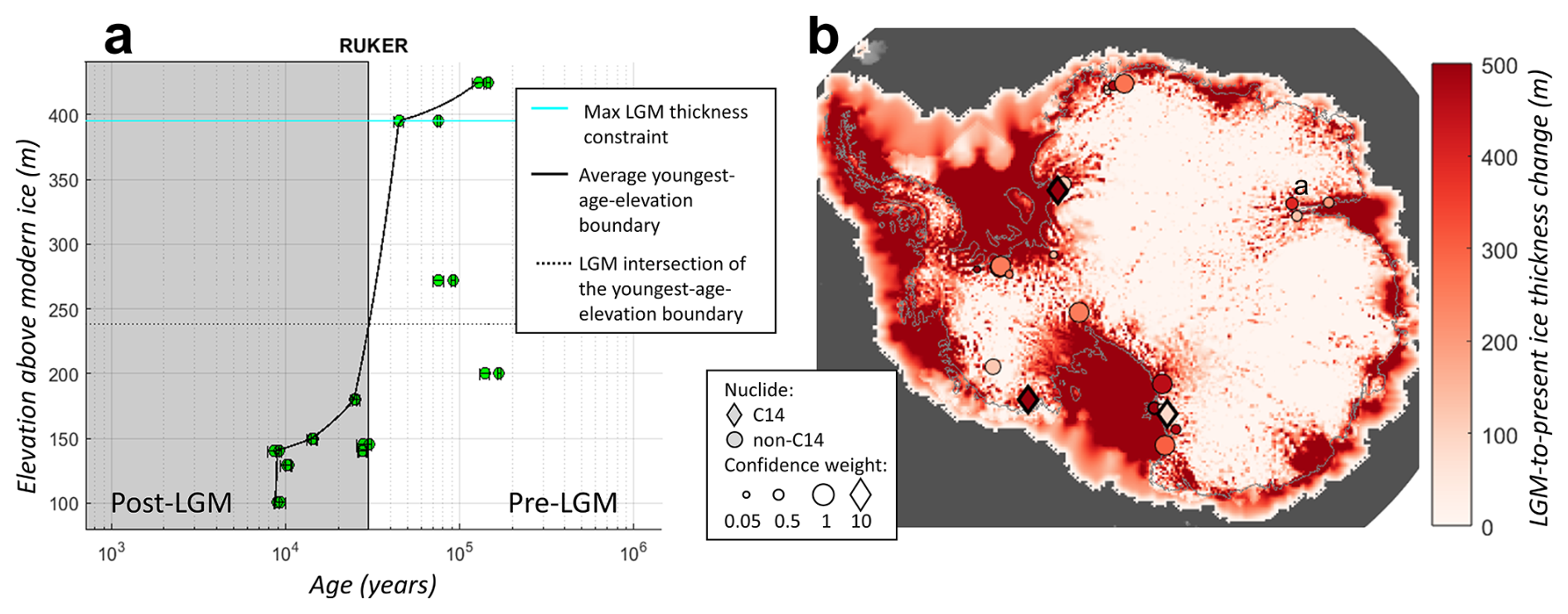
Figure 10 (a) Identifying an LGM maximum ice-thickness-above-present constraint (395 m; cyan line) from a gap between pre- and post-LGM ages at RUKER (Prince Charles Mountains, Mt. Ruker; original data from White et al., 2011). The confidence weighting, based on the total number of samples at the site, is 0.4. (b) Maximum ice thickness constraint data are compared to a model prediction of the same quantity (ice thickness change since the Last Glacial Maximum; shown here from model member 5–0.3–7). Maximum ice thickness constraints are differentiated between ¹⁴C data (diamonds; 3 samples) and non-¹⁴C nuclides (circles; 29 samples). The size of the circle indicates the confidence weighting, described below, from 0–1. Grey contour denotes the modern grounding line.

Both of these methods are more likely to underestimate than overestimate maximum ice thicknesses, because it is theoretically possible that the local LGM ice sheet could have thickened past the identified elevation limit, but neither removed old erratics nor deposited new erratics. Also, short-duration ice thickening events would, presumably, be less likely to deposit erratics. Thus, this methodology is predicated on the assumption that if a post-LGM erratic was present, it was sampled, which of course is not likely to always be true. However, sites with numerous samples are more likely to capture any young erratics that exist, so we therefore assign each site a weight (S_lgm, calculated as the number of samples at the site and then normalized across all sites in the dataset to range from 0 to 1). This assigns a site a higher confidence where there are more samples and thus a greater likelihood that all young erratics at the site were sampled.

Steady-state ¹⁴C concentrations provide clearer and more robust evidence for LGM ice-free conditions. Although ice thickening events of very short duration (hundreds of years) could theoretically have occurred and displaced the ¹⁴C concentration from steady state only at the level of measurement error, the ¹⁴C data provide more reliable constraints on LGM ice thickness compared to other nuclide data (from which we infer LGM exposure simply based on an absence of young ages). Thus, maximum thickness constraints based on ¹⁴C saturation are given a weighting factor S_lgm of 10, an order of magnitude greater confidence compared to the non-¹⁴C constraints.

4.3.2 Quantifying model ice thickness exceedances

At each constraint site, for a given model simulation (both continental and nested domains), we identify the difference between the maximum ice-thickness change over the simulation time, max(H_model), and the identified maximum ice thickness limit above present from exposure age measurements, H_lgm. Thus, the “max thickness exceedance” at a site, m_site,exceed is computed as:

$$\begin{array}{}\text{(6)}& m_{\mathrm{site},\mathrm{exceed}}=max\left(\mathrm{0},\left[\max \left(H_{\mathrm{model}}\right)-H_{\mathrm{lgm}}\right]\right)\end{array}$$

If the model ice thickness never exceeds the maximum ice thickness limit, the site max thickness exceedance is zero. The max thickness exceedance model score is calculated as the mean of the site exceedances multiplied by the site weight S_lgm. Both H_lgm and S_lgm are defined differently across the ¹⁴C and non-¹⁴C thickness constraints.

$$\begin{array}{}\text{(7)}& {\displaystyle }{M}_{\mathrm{exceed}}={\displaystyle \frac{\mathrm{1}}{n}}{\sum }_{i=\mathrm{1}}^n{m}_{\mathrm{site},\mathrm{exceed},i}\ast S_{\mathrm{lgm}}\text{(8)}& {\displaystyle }{H}_{\mathrm{lgm}}=\left\{\begin{array}{ll}{H}_{\mathrm{oldest}\mathrm{samp}}& {}^{\mathrm{14}}\mathrm{C}\\ H_{\mathrm{oldest}\mathrm{samp}\mathrm{above}\mathrm{LGM}\mathrm{intersection}}& \mathrm{non}{-}^{\mathrm{14}}\mathrm{C}\end{array}\right.\text{(9)}& {\displaystyle }{S}_{\mathrm{lgm}}=\left\{\begin{array}{ll}\mathrm{10}& {}^{\mathrm{14}}\mathrm{C}\mathrm{4}\\ \mathrm{0}-\mathrm{1}& \mathrm{non}{-}^{\mathrm{14}}\mathrm{C}\end{array}\right.\end{array}$$

We avoid conflating the model float score with the model exceedance score into one parseable metric (i.e., a “best” model score) for a number of reasons: (1) this masks the complexity of different characteristics of deglaciation that models can replicate (e.g., timing versus amplitude versus rate of thinning), and requires us to impose a static and arbitrary weighting on the importance of thinning amplitude relative to other aspects of deglaciation; (2) model thinning amplitude is more susceptible than other metrics to grid resolution (for example, a grid cell covering more high-elevation mountain-top areas should thin less than a smaller grid cell that excludes mountain peaks surrounding a glacier, for the same regional surface deflation history); and (3) the interpretation of a maximum LGM ice surface elevation from cosmogenic nuclide datasets requires even more uncertain assumptions than reconstructing the pattern of ice surface lowering from a transect of exposure ages (in other words, the ice thickness exceedance misfits are underpinned by different, more uncertain, assumptions, compared to float misfits).

5 Results

In this section we investigate the impact of our methodological choices, specifically, the use of uncurated datasets and the unprecedented high-resolution nested model domains. By implementing the scoring techniques described above for a small ensemble of deglacial ice sheet model simulations, we show that our use of an uncurated data set does not create systematic biases in relation to existing, highly curated, constraint data sets. Therefore, we detect no penalty in taking advantage of an uncurated approach.

We compare model scores between continental simulations and the downscaled high-resolution nested simulations: high-resolution models improve model-data fit, better capturing the thinning patterns across topographically complex regions compared to continental simulations.

5.1 Comparison with a curated dataset

Our model-data evaluation approach is designed to incorporate all available geologic data, with two main aims: to easily assimilate new datasets as they are collected; and to avoid potential interpretation bias. While the interpretation of cosmogenic nuclide measurements can potentially introduce bias, many studies rely on expert assessment to understand individual samples and their geologic context, and removing manual curation will also entail the loss of this expert judgment. It is likely, therefore, this uncurated approach entrains a number of spurious or erroneous data that might have been removed by manual curation but not by automated processing, or misses elements of a complex site. For example, the exposure-age record at DIAMOND (Darwin and Hatherton Glaciers, Diamond Hill) is complex, with multiple nuclides and sample types, and our automated methodology generates a greatly simplified thinning history (Fig. 16a) compared to the in-depth analysis by Hillebrand et al. (2021). Thus, we endeavor to assess whether there is any significant large-scale impact of curation on model scoring and evaluation.

To assess the impact of data curation, we compare model float scores using our uncurated and inclusive ICE-D collection compared to a curated dataset of geologic constraints (Lecavalier et al., 2023). We apply the same preprocessing steps to both our ICE-D dataset and the Levacalier et al. (2023) dataset (i.e., identify sites with > 3 samples spanning > 100 m of elevation change; see Sect. 3.4), and then calculate model float scores for each continental (40-km-resolution) model simulation in our ensemble (Fig. 11). Thus, the only difference in model scores shown in Fig. 11 is therefore the strategy in selecting sites for model/data comparison: our automated preprocessing approach results in 44 sites, whereas the curated Lecavalier et al. (2023) Tier 1 and Tier 2 dataset comprises only 30 of these sites.

While the curated-dataset model scores are overall lower, the overall “ranking” of model simulations remains similar. In other words, both datasets implicate the same best- and worst-scoring simulations. We thus conclude that, although it is not possible to determine whether the curated or uncurated dataset is a priori “better” for model-data comparison, the use of automated data processing rather than manual curation does not appear to introduce a new systematic bias or lead to fundamentally different results. This result is promising for future implementation of a flexible preprocessing approach to assimilate new data as it is collected.

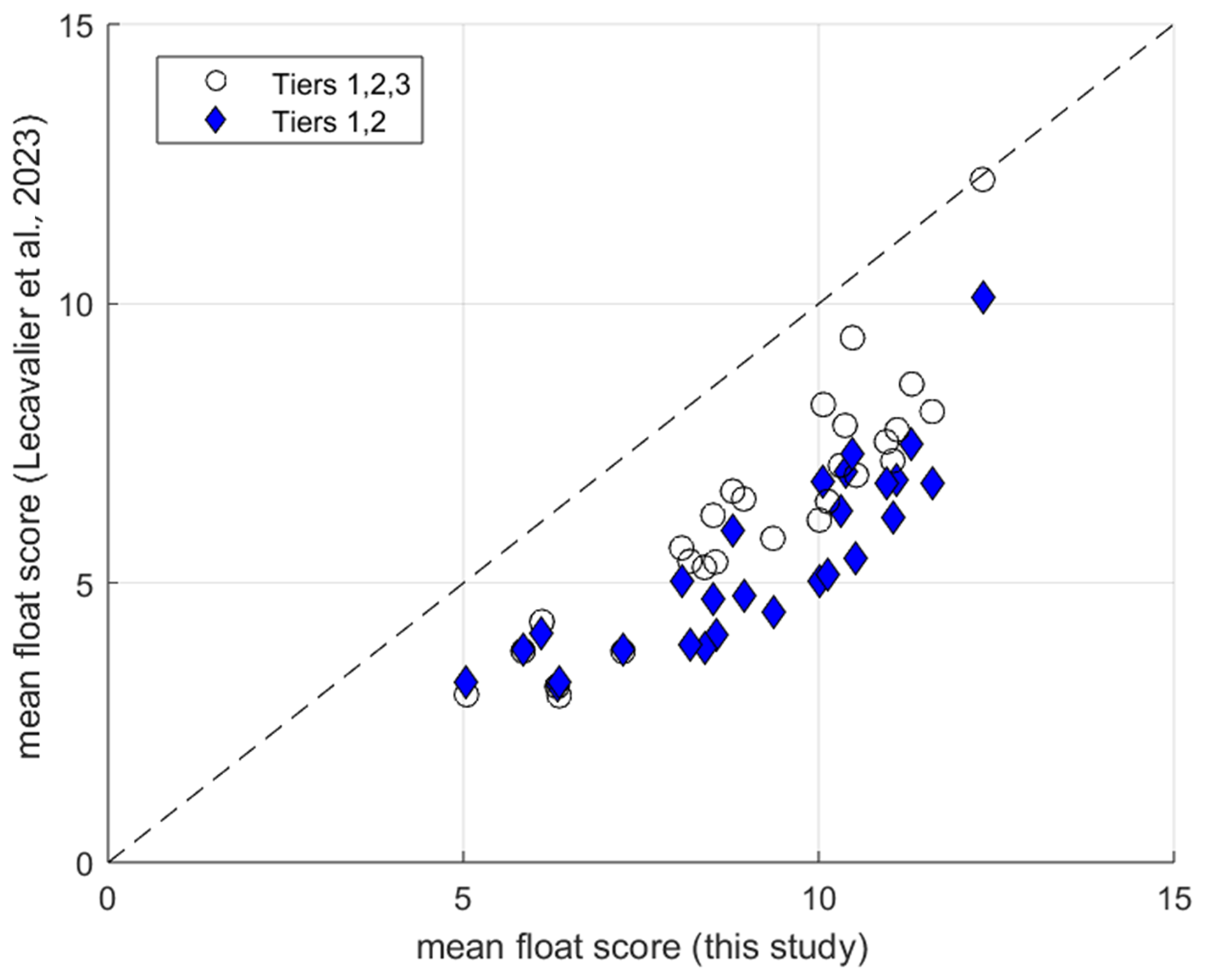
Figure 11 Model float scores for each simulation using either the Lecavalier et al. (2023) curated dataset (y-axis) or the ICE-D all-inclusive dataset (x-axis; this study). Blue diamonds indicate model scores calculated using the Lecavalier et al. dataset with both Tier 1 and Tier 2 constraints, following their methodology (30 sites). We also show the impact of scoring models with all three tiers (38 sites).

5.2 Improvements with high-resolution nested model domains

Continental-scale modeling on millennial timescales requires a relatively coarse model resolution due to computational limitations; at these grid resolutions (20–40 km), nunataks and even entire glaciers that host exposure age measurements are not resolved (Fig. 1), and thus are not well represented by the thinning patterns in our continental-scale model simulations. We performed nested modelling at 2 km grid resolution over smaller domains to investigate the potential improvement in model representation of local deglacial thinning patterns.

We find that the higher-resolution domains better represent local deglacial thinning patterns. This finding is supported by two key observations: (a) the 2 km nested domains are less wrong compared to continental simulations (the 2 km domains improve both model exceedance scores and model float scores for most parameter combinations, Fig. 12); and (b) they are wrong more consistently (have a more consistent time bias, i.e., Fig. 13b compared to Fig. 13a). In other words, applying the best-time-offset shift improves more site misfits across the board.

First, using nested 2 km domains improves model scores (both model float score and model exceedance score) compared to the same simulation at a continental scale resolution (Fig. 12). The overall timing of regional thinning is consistent across model resolution, because the 2 km nested domains are simply downscaling the continental-resolution simulation; thus, the improvement in model performance mainly derives from the improved spatial targeting of glacier thinning. In other words, the higher-resolution domains are revealing differential thinning patterns across glacier troughs and mountains not resolved in the continental scale simulations.

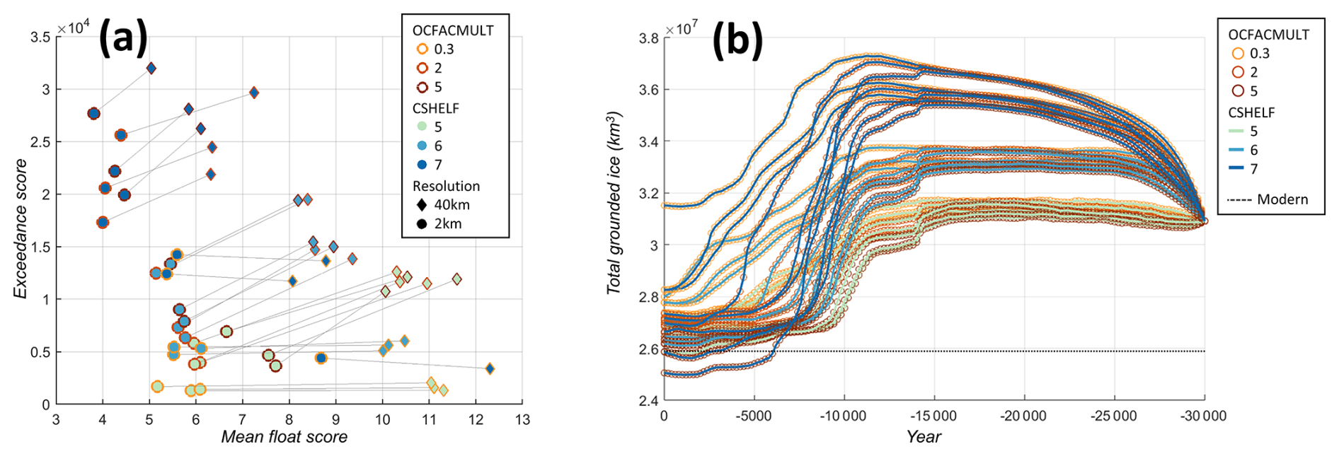
Figure 12 (a) Model exceedance score and model float score for each simulation. Model exceedance scores are summed across 32 sites with geologic max ice thickness constraints. Model float scores are averaged across 49 sites (lumped at a 2 km resolution) or 43 sites (lumped at a 40 km resolution). Marker color and outline color indicate parameter value, and shape/size indicate model grid resolution, connected by a line. TLAPSEPRECIP variation is not denoted; this parameter did not have a systematic trend with respect to model-data fit. (b) Total (40 km resolution continent-wide) grounded ice volume across the ensemble. Modern grounded ice volume is denoted by the black dashed line.

Second, site-by-site model-data discrepancies with the 2 km domains are more consistent compared to the continental simulation, regardless of parameter value. We demonstrate this observation using the best-fit time-offset metric. This metric quantifies how much of an imposed time lag or lead minimizes model-data misfit at any given site. The variation in best-time-offset values across all sites for a given model simulation (i.e., how consistently the model timing is wrong compared to the data) can be represented by the distribution (histogram) of best-time-offsets for all sites (Fig. 13a, b). A numerical simulation where the modeled timing of thinning has to be shifted by a different amount at each site to minimize model/data mismatch within a catchment is a poor representation of the geologic record; this would produce a histogram with a wide ranging distribution of best-time-offsets, reflecting an inconsistent best-time-offset value that varies between sites. A simulation where model/data mismatch at each site can be minimized by shifting the modeled timing of thinning by the same value everywhere within a catchment is a good representation of the geologic record. This suggests that the model is doing a good job at capturing the relative timing of thinning across sites, but is systematically deglaciating too early or too late, likely due to incorrect climatological forcings or parameterizations. This scenario would produce a histogram with a narrow distribution, indicating that the same best-time-offset value improves misfits for most sites in a region. We therefore interpret a tightly distributed histogram of best-time-offset values to indicate a more robust model-data match, because it suggests that model-data misfits are reflecting systematic differences in model parameterizations rather than an incomplete representation of ice dynamics across exposure age sites.

We find that the best-time-offset histograms from the 2 km nested model simulations tend to be more narrowly distributed, as indicated by smaller standard deviations of the best-time-offset distributions (an example of one model ensemble member, Fig. 13a versus b). The 2 km nested models also produce significantly less “best-time-offset outliers” – sites where the best-time-offset value is an end-member value (± 15 kyr) which indicates that model-data fit at a site is so poor that a best-time-offset assessment is not meaningful (outlined in red, in Fig. 13a, b). Figure 13 illustrates the improved ability of these 2 km high-resolution nested simulations to represent deglacial behavior; for all model parameter combinations, the 2 km nested domains produce less best-time-offset “outlier” sites (Fig. 13c), and tighter histograms (more consistent best-time-offset values across sites; Fig. 13d), while maintaining about the same mean best-time-offset compared to the 40 km continental simulation (Fig. 13e). The consistency of mean best-time-offsets across model resolutions simply provides a sanity check that the regional modeled timing of deglaciation is preserved (which we would expect from our downscaling approach, since the 2 km simulations are directly nested within the 40 km continental simulations).

These best-time-offset outliers generally occur at the most interior sites. At these locations, the continental scale model isn't capturing upstream dynamic thinning because (a) if the model does not resolve the glacier system, it cannot represent the resulting dynamic drawdown at that location; and (b) the spatial scale of dynamic drawdown is often subgrid at the 40 km resolution (i.e., a coarse model grid cell averages out the surrounding area and thus produces either too much or too little thinning). At 2 km resolution, the improvements with these two issues result in far fewer best-time-offset outliers.

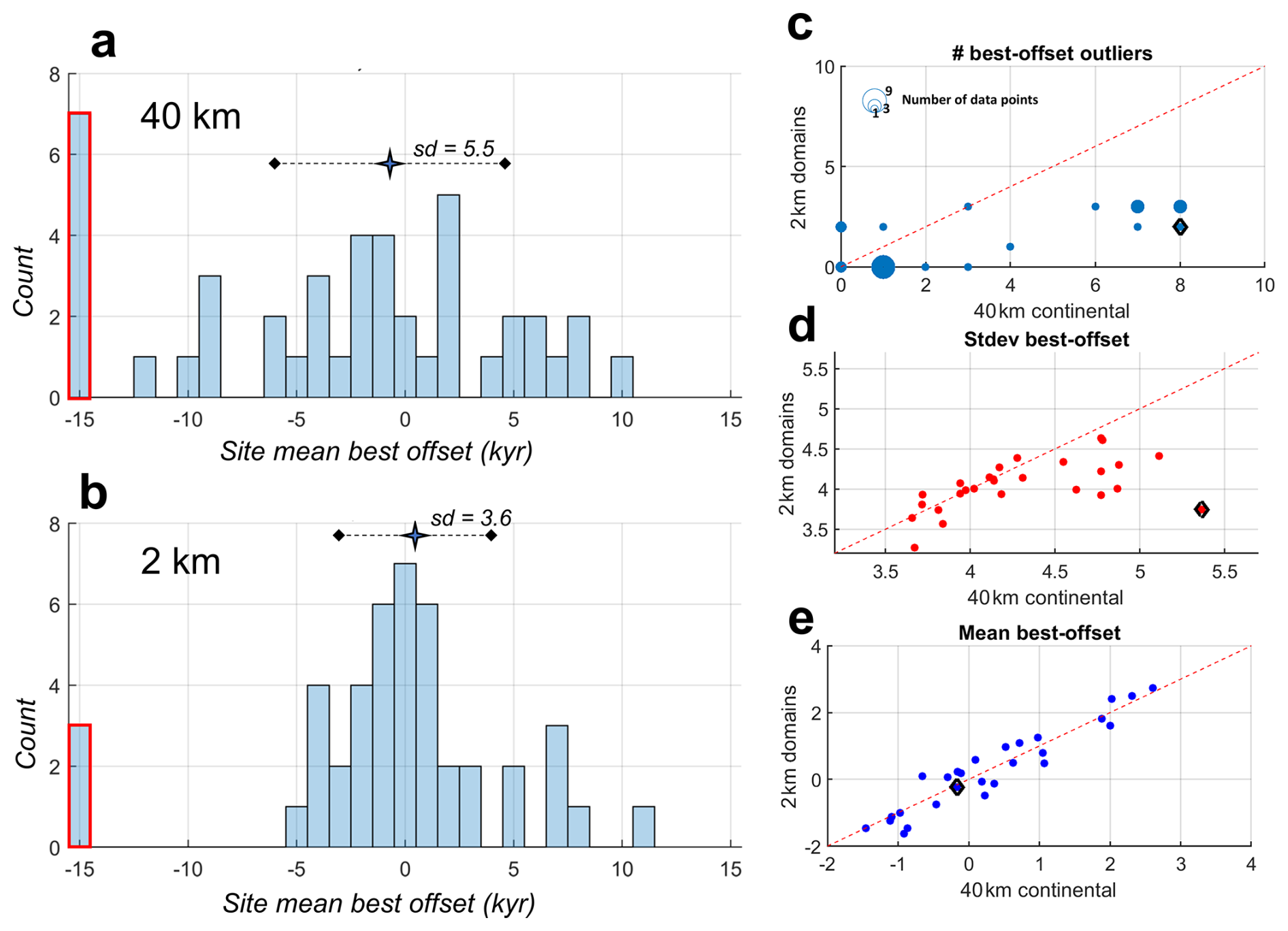
Figure 13 (a, b) Best-time-offset histograms for one ensemble member (5–0.3–7) at both a continental scale (a; 40 km) and nested domain (b; 2 km) grid resolutions. Across the entire model ensemble, using 2 km nested domains over 40 km continental simulations results in (c) fewer outliers, (d) lower standard deviations, while still maintaining (e) similar mean best-time-offset values for each model ensemble member. Standard deviations are calculated after removing outlier sites. This highlights the improvements with 2 km domains: less pathological best-time-offset outliers, which are highlighted in red, and more consistent best-time-offset values as indicated by a tighter histogram distribution and smaller standard deviation). The “5–0.3–7” model member is denoted by a black diamond on the right-hand-side plots (c)–(e).

This analysis of best-time-offset distributions indicates that higher-resolution models provide better context for capturing the heterogeneity in exposure age geologic records. These nested models take the same overall timing of deglaciation across a region and downscale this thinning behavior across discrete glacier troughs and mountains to better resolve the differential thinning patterns that are captured by the existing geologic record. This improvement in representing site-by-site heterogeneity, as well as the overall lower (better) site float misfits and site exceedance misfits, suggest that our 2 km nested model domains provide significant improvements in representing ice dynamics.

6 Discussion

After investigating the application and effectiveness of our new methodology in Sect. 5, here we proceed with interpretations of our model-data evaluation results across the deglacial model ensemble. Based on the demonstrated improvements with higher resolution (Sect. 5.2), we use the 2 km nested domains for model scoring. We explore model/data fit by synthesizing and interpreting our three distinct misfit metrics: the float scoring approach, the ice thickness exceedance approach, and the best-time-offset approach (summarized in Table 1). As presented in Sect. 4, float scoring evaluates the overall shape of the modeled versus measured thinning curves at a site; this shape is determined by a combination of thinning timing, rate, as well as amplitude. Although the model float score reflects poorly on model simulations where model ice sheets do not grow sufficiently thick, it does not explicitly penalize sites where model thinning amplitudes are larger than the amplitude of thinning recorded by terrestrial data. Thus, the ice thickness exceedance score uses a separate dataset of deglacial ice thickness constraints to evaluate the “over-thickening” of each model simulation. Finally, the best-time-offset metric indicates the amount by which a model thinning curve at each site must be horizontally shifted in order to minimize the site float misfit.

Section 6.1 describes a tradeoff between the model float score and model exceedance score: the model simulations that best match the overall shape of the thinning curve at a site (i.e., produce the lowest site float misfit) are not the simulations that best match the amplitude of ice sheet deflation across the last deglaciation (i.e., produce the lowest exceedance score). Section 6.2 leverages the best-time-offset metric to contextualize this timing vs. thickness tradeoff: we find that models with smaller thinning amplitudes (i.e., low exceedance scores) often deglaciate too early, and those with excess ice thickness (i.e., high exceedance scores) persist longer. We also use the best-time-offset approach (i.e., capturing the lingering misfits after applying the best-time-offset value to each site's float misfit approach; Table 1) to eliminate the effect of model-data timing mismatches and evaluate just the modeled rate and pattern of deglaciation. This allows us to investigate whether the timing vs. thickness tradeoff is attributable to a timing mismatch (an issue that could be addressed by improving the climatologies that are used to force the model through time). We interpret the persistence of a residual tradeoff, even after removing timing mismatches, to indicate the presence of lingering challenges associated with modeling the complex patterns of deglaciation as recorded by exposure age data (such as adequate grid resolution).

6.1 No unique “best fit” simulation: tradeoffs between “how fast” and “how thick”

When model simulations are compared to the pattern of thinning revealed by exposure age thinning data (model float score) and the maximum amount of ice thickening during the last glacial cycle recorded by geologic constraints (model exceedance score), a notable gap appears at the bottom left of the plot (e.g., Fig. 12). In other words, no individual model simulation produces both the lowest float score and the lowest exceedance score. While varying additional parameters may result in slightly improved scores, the existing parameter variation here has already produced a wide range of model deglacial behaviors and aligns with existing literature (for example, the range of LGM-to-present ice thickness change simulated in this small ensemble spans the same general range as Albrecht et al., 2020a, in their Fig. 9).

When our higher-resolution nested model domains are implemented, this tradeoff between ice thickness buildup and deglacial thinning rate/timing is diminished yet still persists (Fig. 12). The high-resolution domains result in greater improvements to model float scores compared to model exceedance scores, indicating that the model exceedance scores have lesser sensitivity to model resolution. In other words, nesting improves the ability of the model to match the general shape of exposure-age thinning deglacial curves more than it improves the model ability to represent the amplitude of thinning at our LGM max-thickness constraint sites. We interpret this observation as impetus for future work to improve our understanding of Antarctic LGM thickness constraints, either through adding spatial coverage for exposure age datasets, or including other data types (e.g., geomorphic mapping).

Models with the best (lowest) float scores tend to produce a greater amplitude of ice thickness change than indicated by the geologic record (e.g., OCFACMULT = 5 and CSHELF = 7, top left in Fig. 12). Visual inspection of model results reveals that these large amplitudes of model ice thickness change often improve model-data fit by producing delayed and more rapid deglaciation (compared to models with smaller-amplitude ice thickness change), but these simulations tend to “over-thicken” relative to the maximum ice thickness constraints (i.e., have higher exceedance scores). This modeled ice sheet behavior can be attributed to the impact of stiffer sliding parameter on the continental shelf (CSHELF = 7), supporting larger LGM ice thicknesses, along with heightened sensitivity to ocean melt (OCFACMULT = 5), driving rapid ocean-driven grounding-line retreat. We note that using a different basal friction parameterization with plastic bed rheology (compared to our PSU-ISM power-law treatment) may also produce similar deglacial behavior as lowering the CSHELF value (i.e., smaller LGM ice thicknesses and less abrupt deglacial thinning rates).

Conversely, models with low exceedance scores (e.g., OCFACMULT = 0.3 and CSHELF = 5, bottom right in Fig. 12) have worse float scores; modeled ice thicknesses generally fall short of the thinning amplitudes recorded by the data (and thus the highest-elevation samples are assigned a uniform time gap, specified here as 10 kyr, for calculating site misfit). The third varied parameter TLAPSEPRECIP influences upstream ice thicknesses but had an inconsistent impact on model-data fit. While constraining paleo accumulation patterns is key for robustly reconstructing deglacial ice sheet dynamics, the TLAPSEPRECIP parameter only scales the precipitation field input to the ice sheet model relative to temperature; future work will explore whether alternate time-evolving precipitation histories can generate a more consistent impact on model-data fit.

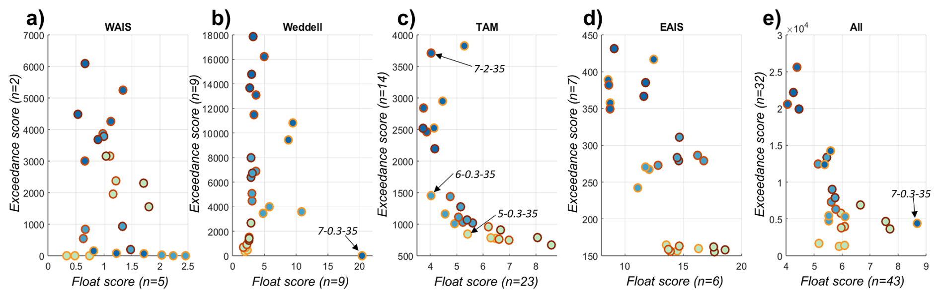
Figure 14 Model float scores and model exceedance scores by region (WAIS: West Antarctic Ice Sheet; Weddell: Weddell Sea region; TAM: Transantarctic Mountains; EAIS: East Antarctic Ice Sheet margin; regions shown in Fig. 1a). Axis labels indicate the number of sites in each region for both model float score and model exceedance score metrics. When all regions are considered (e), scores are identical to the results with 2 km nested domains shown in Fig. 12. Model simulations referred to in the text are labeled here. Circle color and outline color correspond to parameter value, as in Fig. 12.

Given the large differences between regions that might be more or less well-represented in a numerical model across spatial scales – i.e., bathymetry, ocean circulation, and catchment size – we would expect to see different styles of model-data misfit in different sectors. Thus, we further investigate this tradeoff between model float scores and model exceedance scores by partitioning our analysis into different sectors of the Antarctic ice sheet (Fig. 14; see Fig. 1a for region boundaries).

This regional analysis reveals that the timing vs. thickness tradeoff (i.e., tradeoff between model float scores and model exceedance scores) is prominent in East Antarctica (i.e., the Transantarctic Mountain region, as well as the East Antarctic margin though this large region has only a limited number of sites) rather than West Antarctica. In the Transantarctic region, we have acquired the most exposure age data, but it is a highly topographically variable area where the complexity in ice thinning patterns may be subgrid to even the 2 km nested model domains. Systematic mapping of LGM geomorphic limits, or refining and adding exposure age transects across LGM ice thickness extents, may improve our understanding of model performance in this complex region.

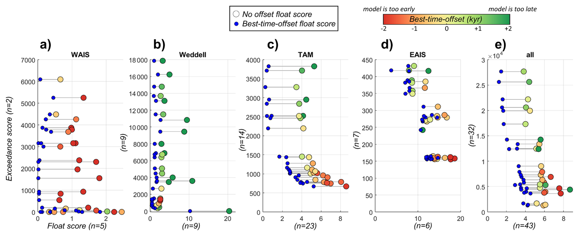
Figure 15 Model float scores with no time offset (same as in Fig. 14), compared to the model best-time-offset scores (the minimum possible float score achieved by shifting the model thinning curves by the best-time-offset value). Each regional model float score is colored with respect to the best-time-offset value (kyr; averaged across all sites in the region) that produces the minimized model best-time-offset score plotted in blue.

Partitioning our analysis by sector, as in Fig. 14, can also highlight major outliers. These outliers are generally associated with large-scale model mismatches to the modern ice sheet configuration. For example, the simulation in Fig. 14b that produces an order-of-magnitude higher model float score than the rest of the ensemble in Weddell Sea (7–0.3–35) never deglaciates to an approximately modern extent, remaining expanded out halfway across the Weddell Sea continental shelf at the modern model time. Thus, although we do not explicitly score model results with respect to the modern ice sheet configuration (see description of our paleo focus in Introduction), model members that produce patently incorrect modern configurations still score poorly against the paleo-data. This is likely due to the many “paleo” data samples with ages of only a few thousand years, which nudge model scores towards realistic present-day configurations. This observation provides reassurance that our scoring approach is able to identify the model runs that best match the deglacial thinning history without sacrificing a reasonable modern configuration.

6.2 Aligning deglacial timing between models and data

The timing of model deglaciation is closely tied to the spatial and temporal evolution of ocean and air temperatures that are input into the model, which, unfortunately, remain highly unconstrained. In this section, we therefore investigate whether the timing vs. thickness tradeoff described above could be attributed to potential systematic errors in the model input climatology. For example, one region may be well-represented by the input climatology if, say, ocean warming in the model climatology co-occurs with the timing of exposure age thinning; whereas another region may require a systematic model/data time offset to best explain thinning patterns.

To address this issue, we leverage the best-time-offset metric. This approach gives the model as many degrees of freedom as possible – allowing the model thinning curve to float in space and time – to see if we can reasonably simulate the general characteristics of deglaciation (rate and pattern of thinning) as recorded by the data. In other words, if we account for some possible model resolution error (e.g., allow the model thinning curve to float vertically), and further “correct” for some hypothetical systematic error in the climatology forcings (allowing the model thinning curve to float horizontally), do any of our models consistently replicate the data-reconstructed shape of ice sheet thinning across all sites?

We can use this analysis to contribute two added layers of information about model/data timing of deglacial thinning. In Fig. 15, we contextualize the patterns revealed by the model float score/model exceedance score plots using information from the best-time-offset metric. We take the regional model float scores from Fig. 14, and additionally plot the regional model best-time-offset scores for each model ensemble (i.e., the minimum possible score – the best score – achieved by vertically and horizontally shifting each model thinning curve). These model best-time-offset scores for each simulation are colored according to the identified best-time-offset value (averaged across the sites in that region) that produced this model best-time-offset score. A best-time-offset close to zero indicates that the model simulation is well-matched to the observed timing of thinning (regardless of the simulation fit to thinning amplitude or rate).

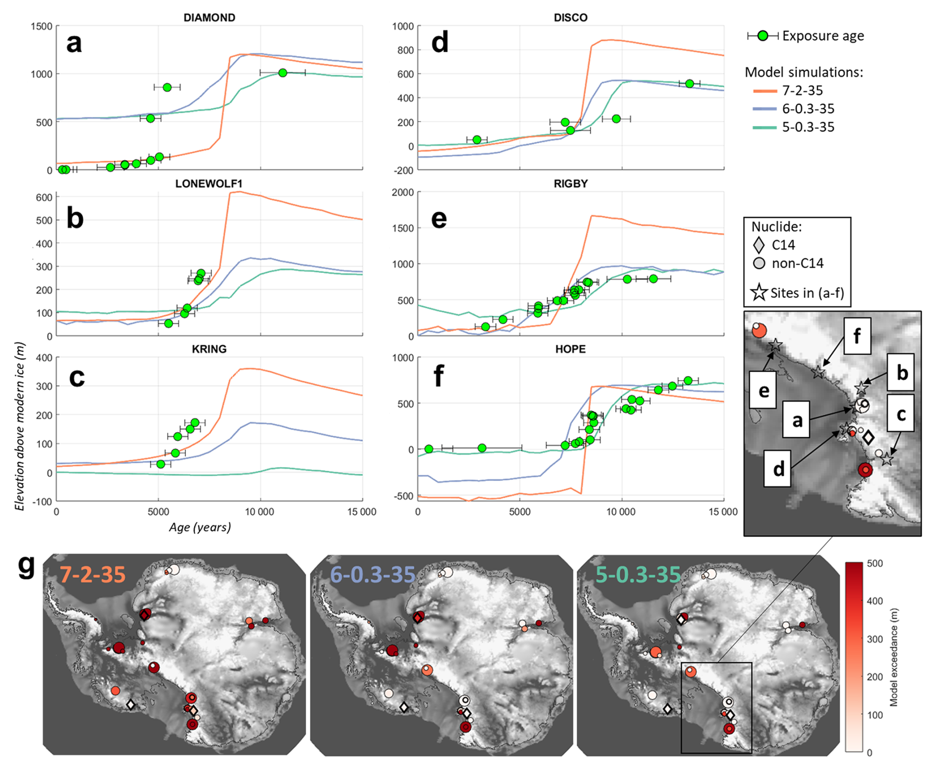
Figure 16 (a–f) At select sites along the Transantarctic Mountains, exposure age thinning histories are compared to model output from three representative ensemble members (model thinning profiles are vertically “floated” to minimize misfit). Original exposure-age data are from Hillebrand et al. (2021) (DIAMOND); Stutz et al. (2023) (LONEWOLF1); Stutz et al. (2021) (KRING); Anderson et al. (2017) (DISCO); and Spector et al. (2017) (RIGBY, HOPE). Sites (a)–(c) show relatively rapid thinning patterns, while sites (d)–(f) record slower thinning. (g) Maximum ice thickness exceedances are plotted spatially for each model simulation (the color indicates the model over-thickening, in elevation (m), compared to each maximum-ice-thickness geologic constraint. As in Fig. 10b, diamonds denote ¹⁴C constraints, and the size of the scatter plot indicates confidence weight. The dark grey contour denotes the modern grounding line, and greyscale bed elevation shown as the final timestep of each model simulation. Site locations for thinning profiles in (a)–(f) are shown in the inset panel of the Transantarctic Mountains (alongside locations and values of maximum ice thickness exceedances for model simulation 5–0.3–35). These three model simulations are labeled in Fig. 14c.

First, we observe an overall trend, mostly in the Transantarctic and EAIS regions, where the model simulations that tend to deglaciate too early (reds in Fig. 15) also have better (lower) exceedance scores. Modeled ice sheets that build up ice thickness in excess of geologic constraints, with worse (higher) exceedance scores, tend to persist for longer into the deglacial period. Thinning curves at these sites must be offset by a few kyr to maximize model fit to the data (positive best-time-offset values; greens in Fig. 15). Thus, combining these three metrics for model/data fit reveals that models with smaller thinning amplitudes often deglaciate too early compared to the exposure age records, while those with excess ice thickness persist longer but better match the measured thinning patterns (lower model float scores).

This behavior can also be visualized in Fig. 16, which shows three simulated thinning curves for select Transantarctic sites; model member 7–2–35 overthickens, simulating a delayed timing of thinning compared to the 5–0.3–35 model which shows a smaller amplitude change and an earlier onset of thinning.

However, we find that this timing difference does not fully explain the observed tradeoff between model float scores and model exceedance scores. When we eliminate the effect of model/data timing mismatches (by considering just the minimized model float scores), the issue persists: no individual model simulation produces the model best-time-offset score and the best model exceedance score for the entire continent (Fig. 15). Therefore, this tradeoff stems from model-data mismatches with respect to just the slope and shape of the thinning curve. In some Antarctic regions (e.g., WAIS, and Weddell, although there are limited data in these areas), model simulations can approach a perfect model best-time-offset score without over-thickening; but in the Transantarctic Mountains, no one model simulation is able to produce both a low float score and a low exceedance score (even after eliminating any impact of a timing mismatch). This reflects an inherent gap in realistic model representation of ice thinning at the spatial scales recorded by exposure age data.

In the TAM region, models that accurately replicate the steep thinning patterns that occur at some sites, correspondingly produce too-steep thinning curves at sites where data indicate slower or lower-amplitude thinning (for example, model simulation 7–2–35 matches the steepness of thinning at DIAMOND, LONEWOLF1, KRING sites in Fig. 16a, but correspondingly produces steep thinning at sites where slower thinning is recorded, e.g., DISCO, RIGBY, HOPE sites in Fig. 16b). This model member that replicates the steep thinning patterns also exceeds almost all of the compiled geologic max-ice-thickness constraints (7–2–35 in Fig. 16d). Conversely, models can better match the flatter thinning curves at some sites but not produce sufficient amplitude of change recorded at other sites (for example, model simulation 5–0.3–35 in Fig. 16a and b). This simulation provides a much better match to the total amplitude of deglacial thinning (5–0.3–35 in Fig. 16d) and thus a much lower (better) exceedance score.

The lingering disconnect between models and data in the TAM region suggests that, despite the significant improvements in model representation of complex ice dynamics using our 2-km-resolution domains (Sect. 5.2), some impactful glacial processes may be sub-grid even at this resolution. This disconnect may also reflect other sources of uncertainty such as poorly represented model physics or model spatial input fields (such as basal friction or climatic forcings), or any large-scale inaccuracy in the continental-scale ice dynamics that provide boundary conditions for the high-resolution nested domains. Because no single model simulation can reproduce the thinning patterns across all sites, even given key parameter variation and two degrees of freedom (vertically and temporally; Fig. 15), this remaining model-data misfit reflects an inherent gap in realistic model representation of ice thinning at the spatial scales recorded in exposure age data. Future work on improving LGM max-thickness constraints may resolve this lingering tradeoff.

7 Conclusions

We present a model-data evaluation framework for benchmarking numerical model simulations with exposure age measurements of ice sheet deflation. We draw on publicly available geologic databases and develop automated methodologies, rather than manual curation, to establish comprehensive geologic constraints for model evaluation. We find that a programmatic approach to data identification and analysis does not create a systematic bias in model evaluation compared to existing manually curated datasets, which is important because the use of uncurated datasets improves data utilization and facilitates rapid and efficient assimilation of newly collected geologic data.

Implementing high-resolution model domains, nested within continental simulations, provides improved representation of differential thinning patterns across glacier troughs and mountains that are not resolved in continental scale simulations. Modeled ice sheet thinning histories from these 2-km-resolution nested model domains reveal a marked improvement in model fit to the observed terrestrial exposure age records compared to the continent-wide simulations. This innovation closes the spatial gap between continental scale model output and mountain-side geologic information, which has challenged previous efforts at model-data comparison.

We further develop model-data alignment techniques to isolate and extract the same specific quantities that are consistent across both numerical simulations and exposure age reconstructions. This improved alignment allows us to build a suite of model-data evaluation metrics built on direct comparisons of thinning behavior.

By exploring a range of model diagnostics derived from the model-data comparison exercise, instead of considering only a single misfit statistic, we demonstrate that no single metric for model-data evaluation satisfactorily produces a best-fit result. Different metrics capture different aspects of ice sheet deflation; an attempt to define a single best-fit model simulation based on a combined misfit statistic loses important diagnostic information. A combination of metrics – assessing the timing, rate, and amplitude of ice sheet thinning – sheds light on different aspects of model ability to reconstruct deglacial ice sheet behavior.

Appendix A: Code and data availability

A1 Access and interface with model-data scoring methodology via a GHub tool

A model-data evaluation toolkit is publicly available via the GHub server (https://theghub.org/tools/modeldatathin; Halberstadt et al., 2025). This tool provides hands-on, interactive access for evaluating model performance at specific sites around Antarctica, especially where exposure-age data have been collected. The tool extracts modeled ice thinning histories at any given site around Antarctica, spanning the last deglaciation. If the specified site contains cosmogenic nuclide exposure-age measurements of ice surface deflation, the tool plots and calculates a site misfit for each selected model based on the methodologies described in this work. Users specify the site location where the model ice sheet history is extracted (ICE-D site, or a lat/lon value anywhere over Antarctica), and select which model simulation(s) to plot and score, as well as model grid resolution (nested or continental-scale).

Below we present an example of using this tool to investigate which model simulation best matches a site of interest (say, RIGBY). For each model simulation selected by the user, model-data misfits are summed across each sample at the site, and the total model score is tabulated. Model thickness profiles, extracted at the specified site location, are plotted for all selected model simulations (colors randomly assigned). The model output file at the specified resolution (the continental domain, or the 2 km nested domain over the specified site of interest) can be directly downloaded by clicking “Download netcdfs” shown in the image below.

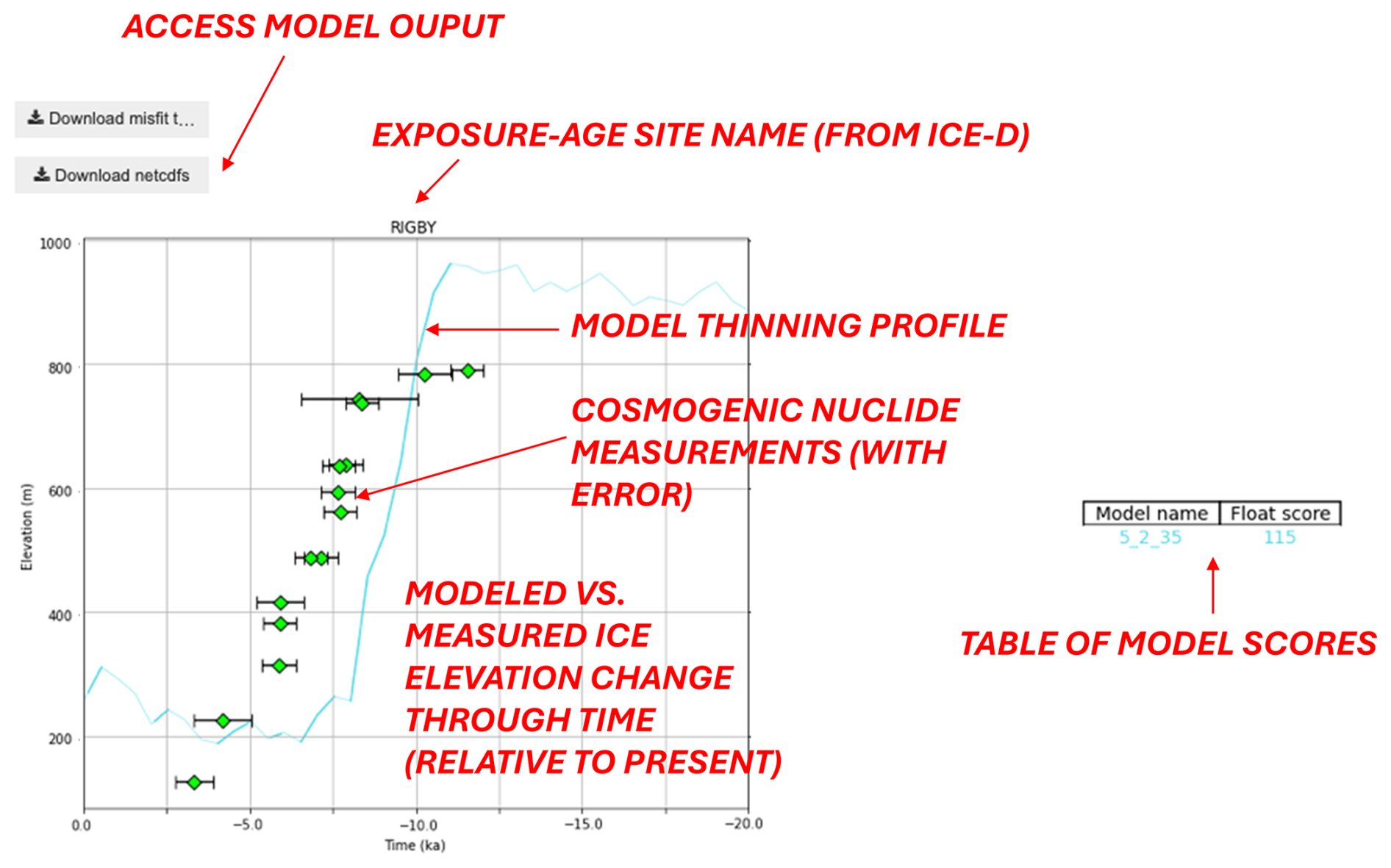
Figure A1 Model thinning at a selected site RIGBY (original data from Spector et al., 2017), compared to the profile of youngest-age-elevation samples at that site. Error bar width denotes the 1σ standard deviation of the Monte Carlo youngest age/elevation space. Model-data misfit at each sample is calculated and the sum is tabulated.

When multiple model simulations are assessed, the user can easily identify which model best fits the thinning pattern recorded at the site of interest.

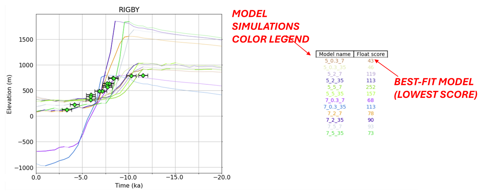
Figure A2 As in Fig. A1, but with multiple model simulations of thinning at the selected site.

Model simulations are, by default, evaluated using the “float scoring metric”, where the model ice thickness curve is vertically offset (“floats”) to minimize model-data misfit. This approach is motivated by issues with aligning model thickness change to a modern baseline, due to model resolution issues (Sect. 4.1.2). A more traditionally used “height scoring metric” (where model ice thickness changes are registered to the modern model ice surface, and the model thinning curve is not permitted to “float” vertically) can be selected in the dropdown menu under “Misfit calculations”. Users can also optionally specify the “uniform time gap” value (Sect. 4.2.3; set at 10 kyr as a default) which allows users to adjust the impact of outlier samples where the measured thinning curve is higher-amplitude than the modeled thinning curve.

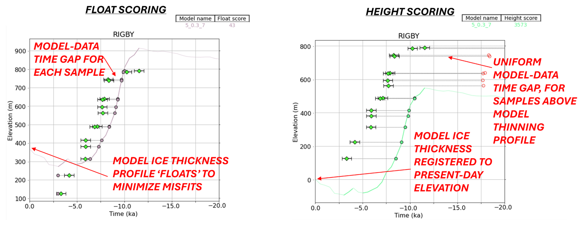
Figure A3 The model-data time gap which is used to calculate sample misfit (Sect. 4.2.1) is plotted as a horizontal bar for a float scoring (left) or height scoring (right) approach. Samples that fall above the model thinning curve are assigned a uniform time gap Δt_u of 10 kyr.

Note that when an ICE-D site is selected, all samples are queried from the database. However, cosmogenic nuclide datasets are often plagued by an old bias. Models should be scored using only the youngest age-elevation samples (Sect. 3.4), which theoretically reflect the progressive exposure of the site as the ice sheet deglaciated. Selecting the option “Calculate and use only the youngest age-elevation-bounding samples” will apply an automated script to identify these youngest samples (though this process can take up to about 15 min to compute).

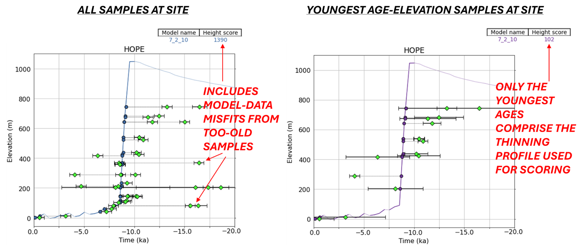
Figure A4 Site misfits are calculated by summing the sample misfits; therefore, using every measured sample at a selected site (left) produces a worse and less representative model score than selecting and proceeding with model-data comparison using just the youngest-age-elevation-bounding samples (right). Original data from HOPE are also from Spector et al. (2017).

A2 Archived geologic constraint datasets

Although the data selection and analysis procedure is implemented as a code that can be applied to the current state of the ICE-D database (as in the publicly accessible GHub tool, see section above), we archive several intermediate steps from the data extraction we performed on 24 April 2024 that was used for the analyses in the paper (Supplement).

During our data preprocessing, as described in Sect. 3.3, we lumped together sites that located within the same model grid cell (combining sample elevation above the modern ice surface, rather than absolute elevation) in order to compare the model thinning history at a grid cell against all of the appropriate corresponding geologic information. This produces a geochronological constraint dataset unique to each model grid resolution. We therefore archive two constraint datasets here (in MATLAB “structure” file format), one for each model resolution (2 km or 40 km), tabulating the youngest age/elevation samples at each site that were used to score model simulations with the specified grid resolution. For each sample, the uncertainty is given as the age range across the Monte Carlo “cloud” at any given elevation (the 1σ range; Fig. 2d), or the minimum geologic uncertainty, whichever is larger, as described in the main text.

We also archive the last-glacial-cycle maximum-thickness constraint dataset (Sect. 4.3), based on data extracted from ICE-D and analyzed on 14 March 2024.

A3 Accessing model output

Both continental-scale and nested model output files can be plotted, queried, and downloaded via the publicly available GHub tool (see above). This allows a user to not only identify the best-fit model simulation to a site of interest, but also to directly leverage model output to explore the regional context that is associated with the thinning at their site of interest. Model output can also be accessed and downloaded in bulk through the Zenodo data record (https://zenodo.org/records/15284166, Halberstadt et al., 2025).