Effects of snow redistribution parameterization on simulated snow thickness validated by MOSAiC observations

Snow plays a critical role in the mass and energy balance of sea ice through its insulating properties and high albedo. Based on observations from the Multidisciplinary Drifting Observatory for the Study of Arctic Climate (MOSAiC) campaign, we assess the influence of two Icepack snow redistribution parameterizations, bulk redistribution and blowing snow redistribution, on snow thickness simulations using the Icepack column model. Our results show that, without snow redistribution, snow thickness is overestimated in winter and spring. The bulk redistribution scheme slightly reduces snow accumulation, while the blowing snow scheme further increases agreement with observations but still overestimates snow accumulation during major snowfall events. Sensitivity experiments indicate that setting p=4, corresponding to a ridged-to-level snow mass ratio of 5, in the bulk redistribution scheme yields the best agreement with snow observations (mean absolute error (MAE) reduced by approximately 73 % relative to the baseline bulk experiment). In the blowing snow scheme, the snow erosion coefficient is treated as an effective tuning parameter. When observed sea ice concentration is prescribed, setting the snow erosion coefficient to $\mathrm{2.4}\times {\mathrm{10}}^{-\mathrm{5}}$ produces simulated accumulated snow loss to leads consistent with observations and improves the simulated snow thickness (MAE reduced by approximately 51 % relative to the original blowing snow experiment). This study provides new insights into snow thickness simulation and the parameterization of snow redistribution, offering valuable guidance for improving modeling of snow thickness on Arctic sea ice.

1 Introduction

Snow cover on sea ice exerts a critical influence on the mass and energy balance of the ice through its high albedo and strong insulating properties (Callaghan et al., 2011; Maykut and Untersteiner, 1971; Webster et al., 2018). Its impact, however, is multifaceted and seasonally variable. In winter, snow insulates sea ice from the atmosphere, suppressing ice growth. In summer, the presence of snow generally increases surface albedo and can delay the onset of surface melt; once melting begins, snowmelt can contribute to meltwater production and melt-pond formation, enhancing solar energy absorption (Eicken et al., 2004; Perovich et al., 2002; Polashenski et al., 2012). Snow accumulation can also lead to flooding and the formation of snow-ice, a process well documented on Antarctic first-year ice (Jeffries et al., 2001; Leppäranta, 1983; Maksym and Jeffries, 2000; Massom et al., 2001) and occasionally observed in the Arctic with the ongoing thinning of sea ice (Kwok, 2018; Granskog et al., 2017; Merkouriadi et al., 2017, 2020). Additionally, summer snow meltwater can percolate into the snowpack and refreeze as superimposed ice, further contributing to sea ice mass (Cheng et al., 2003; Eicken et al., 2004; Wang et al., 2015). Therefore, an accurate representation of snow thickness is essential for improving sea ice modeling and evolution.

The spatial distribution of snow thickness on sea ice is primarily controlled by snowfall (Wagner et al., 2022), but it is also strongly shaped by wind-driven snow redistribution. Strong winds can lift snow particles from the surface, and a portion of these suspended particles fall into open leads (Lecomte et al., 2015; Leonard and Maksym, 2011; Petty et al., 2018), while the remaining particles are redistributed on the snow surface, thereby altering the spatial distribution of snow thickness and affecting the mass and energy balance of the snow (Luo and Zhang, 2022). Blowing snow can also facilitate the sublimation of suspended snow particles (Déry and Yau, 2002; Liston et al., 2020), and studies have shown that under the same atmospheric conditions, the sublimation rate of blowing snow is two orders of magnitude higher than that of a stationary snow surface (Schmidt, 1982). Previous modeling studies have shown that wind-driven redistribution and blowing-snow processes can substantially modify the snow mass budget on polar sea ice through snow transport, sublimation, and redistribution among different ice surface types (Déry and Tremblay, 2004; Chung et al., 2011; Lecomte et al., 2015). Recent satellite-based studies during MOSAiC further indicate that blowing snow was active over Arctic sea ice and may represent an important sink in the snow-on-sea-ice budget (Robinson et al., 2025, 2026).

Observational studies highlight the importance of these processes for the snow mass budget. In the Southern Ocean, Leonard and Maksym (2011) suggested that approximately half of the precipitation over sea ice could be lost to leads under the observed conditions. During the MOSAiC expedition, observations indicate that under typical winter conditions, leads have a minimal impact on the snow mass balance, but when snowfall occurs alongside strong winds and high temperatures, 65 %–100 % of the recent snowfall can fall into open leads (Clemens-Sewall et al., 2023), as strong winds promote snow redistribution and higher temperatures prevent rapid lead refreezing. Recent work has also emphasized that snow sinks on level sea ice can vary strongly with atmospheric forcing, surface state, and ice conditions (Merkouriadi et al., 2025). Parameterizations of snow redistribution by wind have been applied in climate models (Lecomte et al., 2015) and reanalysis-forced reconstruction models of snow evolution on sea ice, such as NESOSIM (Petty et al., 2018). However, these approaches typically rely on simplified assumptions or tuning parameters and have not been extensively evaluated against detailed observations.

In Icepack 1.3.2, the empirical coefficients in the snow redistribution parameterization remain uncertain and have not been systematically constrained using recent MOSAiC observations. Although newer versions of Icepack have since been released, we used Icepack 1.3.2 to maintain consistency with the model configuration used in this study and focused on evaluating the snow redistribution parameterizations implemented in that version. Previous studies using the Icepack model have examined the performance of snow redistribution processes in simulating snow thickness (Hao et al., 2025; Zhao et al., 2025). In particular, Zhao et al. (2025) evaluated snow evolution along the MOSAiC drift trajectory using Icepack configurations with no redistribution, bulk redistribution, and blowing-snow redistribution, highlighting the importance of snow redistribution and melt-pond schemes for simulated sea ice thickness. However, the lack of accurate snowfall observations and measurements of snow blown into open leads introduces uncertainty in snow thickness simulations. In this study, we use atmospheric, oceanic and sea ice observations from the MOSAiC expedition to evaluate Icepack's snow redistribution, examine its impact on simulated Arctic snow thickness and explore avenues for further optimization. Section 2 describes the data and methods. Section 3 presents the performance of different snow redistribution processes on snow thickness simulation (Sect. 3.1) and proposes improvements to the snow redistribution parameterization (Sect. 3.2). Sections 4 and 5 provide the discussion and conclusions.

2 Data and methods

2.1 Icepack

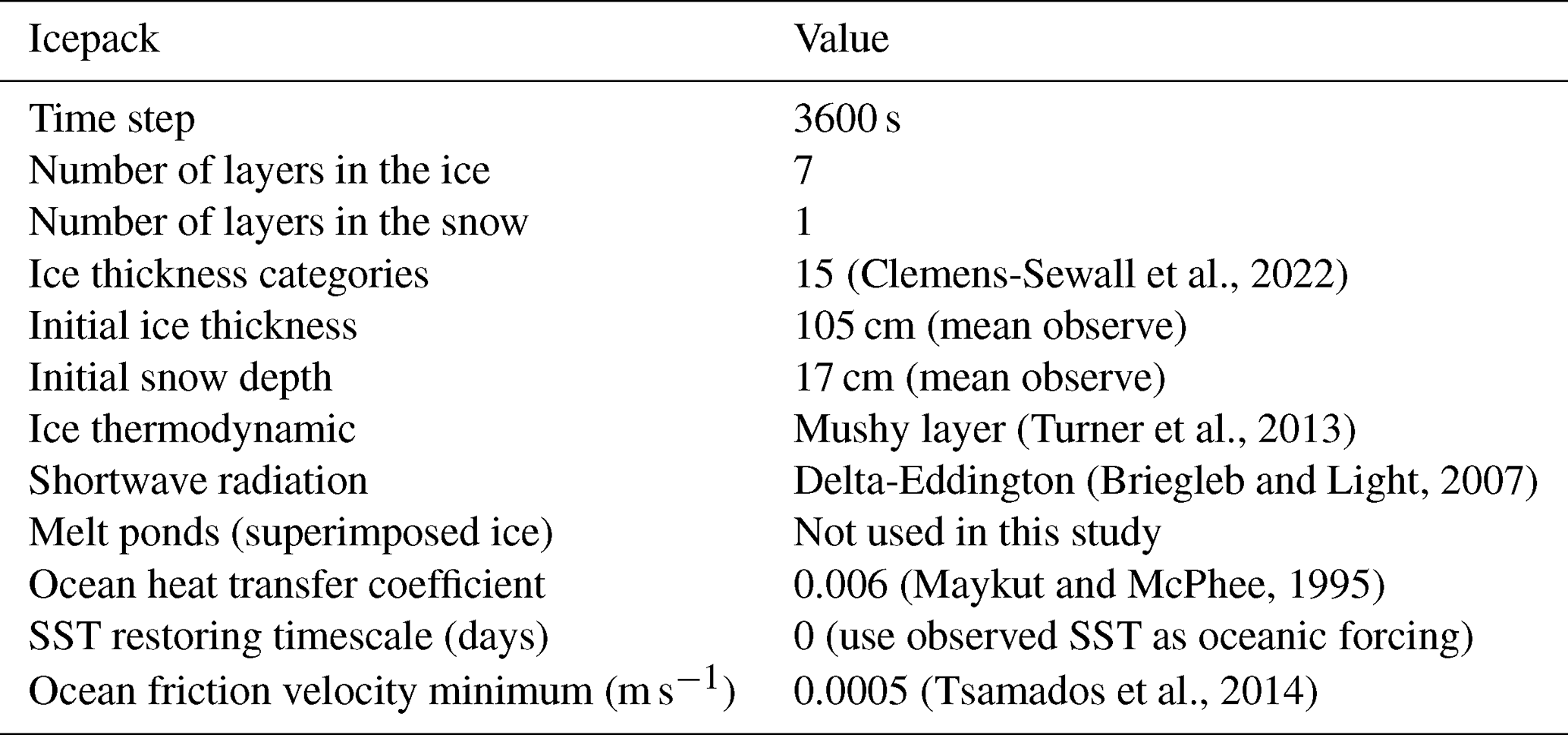
The Icepack single-column model is a state-of-the-art numerical model managed by the CICE consortium. It contains physical processes that affect sea ice thickness within a single grid cell without reference to adjacent grid cells. Subgrid ice classes are described by dividing the ice area fraction into discrete thickness categories within the single Icepack column. The model solves a set of equations that represent ice dynamics, thermodynamics, and mechanical redistribution (ridging). In this single-column configuration, lateral interactions with adjacent grid cells are not represented; changes in the ridged-ice fraction are handled through the prescribed ice thickness distribution and the mechanical redistribution scheme within the column. This study used Icepack version 1.3.2 (Hunke et al., 2022). The focus is on the effects of snow redistribution parameterization on snow thickness simulation. The Icepack simulation was conducted December 2019 to July 2020. The key model settings and physical parameterizations are summarized in Table 1 (Gu et al., 2022, 2024). In this single-column Icepack configuration, ocean temperature, salinity, and current forcing are prescribed from observations and used as external forcing for the ice column. Snow deposited into leads is treated as an immediate snow mass flux from the ice-snow column to the ocean; however, the resulting freshwater input is not allowed to feed back onto ocean salinity, ocean stratification, or ocean-to-ice heat fluxes. Following Clemens-Sewall et al. (2022), the Icepack ice thickness distribution is divided into 15 categories to more accurately represent the distribution of snow thickness.

Table 1 Detailed options of physical parameterizations and model settings for Icepack. SST signifies sea surface temperature.

2.2 Observational data

For this study, we used a comprehensive set of observational data encompassing atmospheric, oceanic, sea ice and snow thickness measurements collected during the MOSAiC expedition, which took place from October 2019 to September 2020. All observations were obtained within an area of approximately 15 km (Bliss et al., 2023). The atmospheric data included the Met City monitoring station and three Atmospheric Surface Flux Stations (Shupe et al., 2022). We used averaged atmospheric data from Met City and three ASFS sites as forcing for Icepack. The variables include downward shortwave and longwave radiation, 2 m air temperature, 2 m specific humidity, and 10 m wind speed. The ASFS 2 m wind speed was extrapolated to 10 m using a power-law relationship with a sea-ice surface roughness length of $\mathrm{1.0}\times {\mathrm{10}}^{-\mathrm{3}}$ m, following the ECMWF-IFS model (Ruti et al., 2008).

Oceanographic data comprised 10 m sea temperature and salinity measurements from eight Conductivity, Temperature, and Depth (CTD) buoys, as well as 3 m sea temperature, salinity, and current velocity data from four autonomous ocean flux buoys. Because all ocean temperature and salinity observations were located within the mixed layer depth (Rabe et al., 2022), the 10 and 3 m measurements were combined to obtain mixed-layer representative time series and then spatially averaged across the buoys. These time-dependent temperature and salinity series were prescribed as external ocean forcing in the Icepack simulations. The observed relative velocities between sea ice and the ocean surface current from the four autonomous ocean flux buoys were used to calculate the friction velocity, which was then used to estimate ocean–ice heat exchange. Although Icepack prescribes friction velocity as a fixed constant by default, we implemented a quadratic drag law following Jenkins et al. (2010), ${u_{*}}^{\mathrm{2}}=c_w{U}^{\mathrm{2}}$, where c_w is the dimensionless ice–ocean drag coefficient and U is the ice velocity relative to the ocean surface current.

The ice opening and closing rates (s⁻¹) are derived from SAR-based sea ice divergence in the Transpolar Drift during MOSAiC 2019/2020 (von Albedyll, 2024), following the method described by Bitz (2026). In addition, precipitation data from the present weather detector (PWD) on the deck of the Polarstern and from the ERA5 reanalysis (Wagner et al., 2022) were used. Precipitation forcing is an important source of uncertainty in the snow-thickness simulations. Following Wagner et al. (2022), we used the average of precipitation from the PWD and ERA5 reanalysis as the model precipitation forcing, because MOSAiC precipitation estimates differ substantially among products and the actual precipitation likely lies between the PWD and ERA5 estimates. The resulting cumulative precipitation from 31 October 2019 to 26 April 2020 is 91 mm, within the observationally constrained range reported by Wagner et al. (2022). Nevertheless, uncertainties in precipitation timing, frequency, and magnitude may contribute to biases in simulated snow accumulation, especially during individual snowfall events.

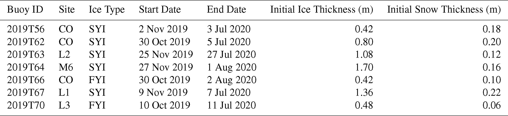
The Icepack was initialized using MOSAiC observations of initial snow thickness and ice thickness from the Snow and Ice Mass Balance (SIMBA) array (Lei et al., 2022). In this study, seven buoys were selected according to their operational periods (Table 2), and their mean snow thickness and mean ice thickness were used to evaluate the simulated snow and ice thickness. According to the site descriptions summarized by Perovich et al. (2023), these buoys were deployed over both first-year ice and second-year ice. Because the Icepack simulations used a fixed snow density of 330 kg m⁻³, whereas the observed snow density varied from approximately 250 to 400 kg m⁻³ (Macfarlane et al., 2023), a direct comparison based only on snow depth would not account for variations in snow mass. Therefore, the observed snow thickness were converted to snow water equivalent (SWE) using fitted SnowMicroPen (SMP) density–SWE relationships (Wagner et al., 2022), allowing the observations and simulations to be compared in terms of snow mass. Although this empirical conversion may introduce additional uncertainty, it provides a more physically consistent basis for evaluating the simulated snow mass. Daily sea ice concentration data were obtained from the Advanced Microwave Scanning Radiometer 2 (AMSR2) using the Arctic Sea Ice (ASI) algorithm (Spreen et al., 2008) developed at the University of Bremen, at a spatial resolution of 3.125 km.

Table 2 Characteristics of the seven MOSAiC Snow and Ice Mass Balance Array (SIMBA) buoys used in this study, including deployment site, sea-ice type, observation period, and initial snow and ice conditions. The selected buoys were deployed over both first-year ice (FYI) and second-year ice (SYI) during the MOSAiC expedition (Perovich et al., 2023; Salganik et al., 2023). CO refers to the Central Observatory, L1–L3 are Local Scale Distributed Network sites located within a few kilometers of the Central Observatory, and M6 is a Mesoscale Distributed Network site located tens of kilometers from the Central Observatory.

2.3 Snow redistribution physical process

In Icepack, snow mass evolves through snowfall, condensation, melting, sublimation, snow-ice formation, and wind-driven processes (Hunke et al., 2022). Icepack includes two snow redistribution processes: bulk redistribution and snwITDrdg redistribution. In the bulk redistribution scheme, the parameterization is motivated by SHEBA observations showing that snow in the vicinity of ice ridges was approximately 30 % greater than that on level ice (Sturm et al., 2002). This observed contrast may result from several physical processes, including wind-driven redistribution of snow from level ice toward ridged areas, snow loss into leads, sublimation, and snow incorporation during ridging. In Icepack, these unresolved processes are represented in a simplified way by assuming that a fraction of incoming snowfall over level ice is instantaneously diverted into the ocean through leads, thereby reducing the effective snowfall contributing to snow accumulation on level ice (Hunke et al., 2022). Mathematically, the amount of snow entering the leads is given by:

$$\begin{array}{}\text{(1)}& s_{\mathrm{f}}^{\prime }=s_{\mathrm{f}}\left[a_{\mathrm{lvl}}\left({\displaystyle \frac{p}{\mathrm{1}+p}}\right)\right]\end{array}$$

where s_f is the snowfall rate, a_lvl is the area of the level ice within a grid cell, and 1+p represents the ratio of snow mass on ridged ice to that on level ice, while p represents the excess snow mass on ridged ice relative to level ice.

In the processes of snwITDrdg redistribution, the erosion rate of the snow is expressed as:

$$\begin{array}{}\text{(2)}& {\mathrm{\Phi }}_{\mathrm{local}}^T={\left({\displaystyle \frac{\partial m}{\partial t}}\right)}_{\mathrm{erosion}}=-{\displaystyle \frac{\mathit{\gamma }}{\mathit{\sigma }\text{ITD}}}\left(V-V^{*}\right){\displaystyle \frac{{\mathit{\rho }}_{\max }-{\mathit{\rho }}_{\mathrm{s}}}{{\mathit{\rho }}_{\max }}}\end{array}$$

where ρ_max and ρ_s are the maximum snow density and the effective snow density in Icepack, respectively. The value of ρ_max is set to 400 kg m⁻³ (Macfarlane et al., 2023). When erosion begins, snow particles start to suspend when the instantaneous wind speed V exceeds a threshold (V^*). σITD is the standard deviation of the sea ice thickness distribution within a grid cell (Hunke et al., 2022). γ is a tuning coefficient that modulates the snow erosion rate, set to $\mathrm{1}\times {\mathrm{10}}^{-\mathrm{5}}$ kg m⁻² (Lecomte et al., 2015). In Icepack, the default/background snow density is 330 kg m⁻³, but the snwITDrdg scheme can also account for wind-induced compaction of the upper snow layer into denser wind slabs. The threshold V^* is calculated from the effective snow density following Lecomte et al. (2013), using ${\mathit{\rho }}_{\mathrm{s}}=\mathrm{174}+\mathrm{44.6}{V}^{*}$. Therefore, when ρ_s=330 kg m⁻³, V^* is approximately 3.5 m s⁻¹. This V^* represents the wind speed associated with compacting snow to the effective density used in the parameterization. Further details are provided in the Icepack technical documentation (Hunke et al., 2022).

The remaining suspended snow particles are redistributed over the ice surface as:

$$\begin{array}{}\text{(3)}& {\mathrm{\Phi }}_{\mathrm{local}}^R\mathrm{\Delta }t=a_{\mathrm{i}}\left(\mathrm{1}-f\right){\mathrm{\Phi }}_{\mathrm{local}}^T\mathrm{\Delta }t\end{array}$$

Where f represents the fraction of suspended snow particles lost within the leads (Lecomte et al., 2013):

$$\begin{array}{}\text{(4)}& f=\left(\mathrm{1}-a_{\mathrm{i}}\right)\exp \left({\displaystyle \frac{-{\mathit{\sigma }}_{\mathrm{ITD}}}{{\mathit{\sigma }}_{\mathrm{ref}}}}\right)\end{array}$$

Where σ_ref=1 m, and a_i is the area of the ice within a grid cell. Here σ_ref is a reference scale for the standard deviation of the ice thickness distribution. The exponential term indicates that snow loss to leads decreases as σ_ITD increases. Physically, a larger σ_ITD reflects more ridged or deformed ice, which can shelter drifting snow and promote snow accumulation near ridges, thereby reducing the fraction of suspended snow transported into leads. The remaining suspended snow is redistributed locally among the ice thickness categories, preferentially increasing snow accumulation over ridged/deformed ice while reducing snow over more exposed level ice.

In addition to the redistribution mechanisms described above, the snwITDrdg scheme relies on several simplifying assumptions that influence the representation of blowing-snow processes in Icepack. Snow loss to leads therefore occurs both through direct snowfall onto open water when sea ice concentration is below unity and through wind-driven snow erosion when wind speed exceeds a threshold. Icepack assumes local conservation of snow mass during blowing-snow redistribution, neglecting non-local transport between grid cells (Lecomte et al., 2015). Snow redistribution directly modifies the snow thickness associated with each ice thickness category and therefore affects the thermodynamic evolution of snow and ice. However, because Icepack assumes a uniform snow thickness within each category, subgrid-scale spatial heterogeneity in snow redistribution is not explicitly resolved. The uniform snow-thickness assumption applies to the thermodynamic calculation within each ice thickness category, whereas the redistribution and radiation calculations account for the effects of level and ridged ice fractions. Although snow thickness directly affects the thermodynamic mass balance, the effects of its spatial variability are primarily represented through the surface radiation scheme, which responds to changes in effective surface fractions (Hunke et al., 2022).

3 Results

3.1 Snow Thickness Simulation Based on Different Snow Redistribution Processes

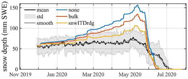
To simulate snow thickness during the MOSAiC period, we force the Icepack sea ice column model with mean atmospheric and oceanic observations. We assess the impact of the snow redistribution parameterization by comparing three Icepack configurations: no-redistribution experiment, bulk redistribution (bulk), and blowing-snow redistribution (snwITDrdg). All snow thickness values are converted to SWE for consistency with observations. Figure 1d shows that observed SWE increased from ∼55 mm in December 2019 to ∼ 65 mm by March 2020, then slightly decreased in April, peaked at 75 mm in May, and rapidly melted as temperatures rose (Fig. 1a), with complete melt by July. The observed ice thickness increased from about 1.0 m in December 2019 to a maximum of about 1.9 m in early June, followed by rapid summer melt, decreasing to ∼1.3 m by the end of July (Fig. 1e).

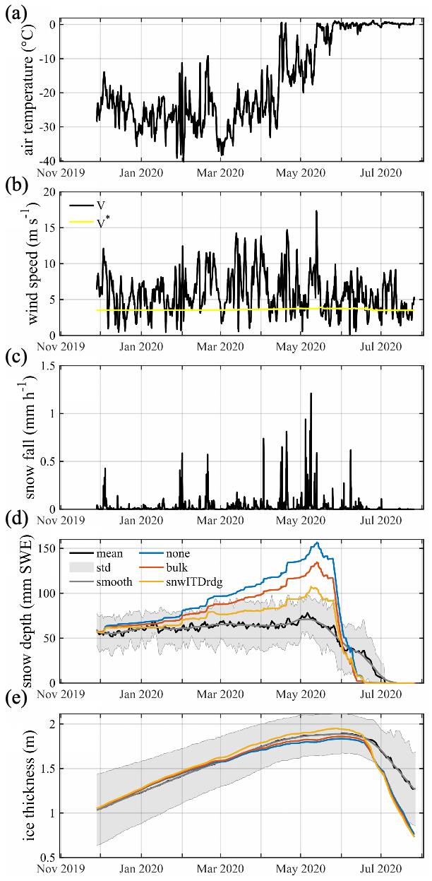
Figure 1 Simulation time series of (a) 2 m air temperature, (b) 10 m wind speed, (c) snowfall, (d) snow thickness, and (e) ice thickness. The black line represents the observation, and the yellow line in (b) represents the wind speed threshold (V^*) for snow erosion and suspension in the snwITDrdg scheme. In (d) and (e), the thick black line and grey shading represent the multi-site mean observations and their standard deviation, respectively, while the gray line indicates the 20 d moving average of the mean observations. The blue, red, and yellow lines represent the snow thickness simulations with no redistribution, bulk redistribution, and snwITDrdg redistribution, respectively.

For the no-redistribution experiment, simulated SWE is overestimated relative to observations starting in mid-January, particularly during periods of snowfall. The simulation peaks at 155 mm on 13 May, compared with the observed corresponding to an overestimation of about 80 mm SWE. It then rapidly melts, with complete melt occurring by 17 June. The bulk scheme reduces snow thickness slightly, but the seasonal trend remains similar, with a peak SWE of approximately 130 mm and a mean absolute error (MAE) of approximately 23 mm SWE before June. In contrast, the snwITDrdg scheme significantly reduces SWE compared with the no-redistribution experiment and bulk scheme, lowering the peak SWE to approximately 105 mm and reducing the MAE to approximately 13 mm SWE before June. According to the parameterization described in Sect. 2.3, snow redistribution is activated when the wind speed exceeds the threshold for snow erosion (∼3.5 m s⁻¹; Fig. 1b). Under these conditions, suspended snow particles are redistributed over the ice surface or deposited into open leads (Lecomte et al., 2013, 2015; Hunke et al., 2022), thereby reducing snow accumulation and bringing the simulated temporal evolution of SWE closer to the observations. However, even with blowing-snow redistribution, simulated snow thickness remains overestimated in winter and spring and melts too rapidly in summer (Fig. 1d), indicating that none of the three default snow redistribution schemes fully reproduces the observed SWE evolution. This remaining bias motivates the parameter optimization of the snow redistribution parameterization presented in the following section.

Compared with the snow thickness simulations, the ice thickness simulations show better agreement with the observations before the onset of summer melt. The spread in simulated ice thickness among experiments is much smaller than the spread in snow thickness. The no-redistribution and bulk redistribution experiments slightly underestimate ice thickness during April to mid-June, while the snwITDrdg experiment exhibits a modest overestimation during this period. After mid-June, all simulations tend to underestimate the observed ice thickness. This bias is likely attributable to the rapid melt of simulated snow thickness during summer, which leads to increased exposure of sea ice to the warm atmosphere (Fig. 1e).

3.2 Optimization of the Snow Redistribution Parameterization

We conduct a series of parameter optimization experiments aimed at improving the performance of the bulk and snwITDrdg snow redistribution schemes. Specifically, we focus on optimizing P, which represents the excess snow mass on ridged ice relative to level ice in the bulk redistribution scheme, as well as the sea ice concentration and the tuning coefficient γ in the snwITDrdg redistribution scheme.

In the bulk redistribution scheme, p is set to 0.3 based on estimates from SHEBA observations conducted during 1997–1998, which suggest that snow thickness on ice ridges is approximately 30 % greater than that on level ice. However, observations during the MOSAiC campaign indicate that large ridges accumulated nearly five times the snow depth of level ice (Itkin et al., 2023). Because this estimate does not include small ridges, which constitute a large fraction of ridged ice, it should be interpreted as an upper-end observational constraint. Therefore, to investigate the sensitivity of the model over an observationally supported range, we increased p from 0.3 to 4.0 to examine its impact on simulated snow and ice thickness. Based on Eq. (1), this range corresponds to $p/(\mathrm{1}+p)$ values from approximately 0.23 to 0.80, so the fraction of snowfall passed to leads is $a_{\mathrm{lvl}}p/(\mathrm{1}+p)$. The mean absolute error was used to evaluate the agreement between simulated and observed SWE before June: $\text{MAE}=\mathrm{1}/n\sum |{\mathrm{SWE}}_{\mathrm{sim}}-{\mathrm{SWE}}_{\mathrm{obs}}|$, where n is the number of data points over the period prior to June. SWE_sim and SWE_obs the simulated and observed SWE, respectively. Therefore, the snow MAE is reported in mm SWE. The same MAE formulation was applied separately to ice thickness, with ice-thickness errors reported in m. The results show that increasing p leads to more snow being redistributed into open leads, thereby reducing the simulated snow thickness (Fig. 2a). The minimum snow thickness MAE (∼6.2 mm) is achieved when p=4 (hereafter referred to as bulkm, Fig. 3b). The simulations with model-simulated and prescribed AMSR2 sea ice concentration show similar sensitivity trends as p increases, with only small differences in accumulated snow loss and SWE MAE. These differences arise because prescribing AMSR2 sea ice concentration slightly modifies the level-ice and lead area fractions used in the bulk redistribution calculation.

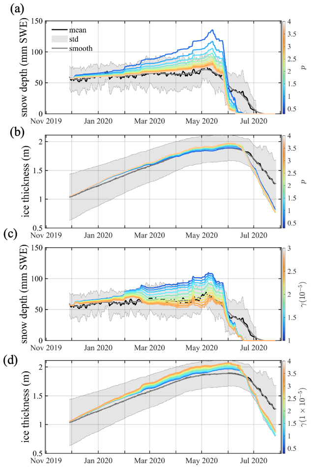
Figure 2 Time series of (a) snow thickness and (b) ice thickness from sensitivity experiments under the bulk redistribution scheme with varying p, where p is the excess snow mass on ridged ice relative to level ice, and (c) snow thickness and (d) ice thickness show the snwITDrdg sensitivity experiments with prescribed AMSR2 sea ice concentration. γ is the tuning coefficient controlling the snow erosion rate. In panels (a) and (b), the 10 colored lines represent sensitivity experiments with p ranging from 0.3 to 4.0. In panels (c) and (d), the 11 colored lines correspond to sensitivity experiments with the γ tuning coefficient ranging from $\mathrm{1}\times {\mathrm{10}}^{-\mathrm{5}}$ to $\mathrm{3}\times {\mathrm{10}}^{-\mathrm{5}}$.

In the snwITDrdg redistribution simulation, an increase in γ represents an increase in the parameterized amount of suspended snow, while a decrease in sea ice concentration enlarges the leads, which provide more open-water area to receive drifting snow. As a result, more snow particles are transported and deposited into these leads. There is a significant bias between the simulated and observed sea ice concentration (Fig. 3a). The simulated sea ice concentration gradually decreased from 0.98 to 0.92 by the end of July, after which it decreases rapidly. The observed sea ice concentration experiences significant reductions both at the end of April and July, reaching as low as 0.7. This increases leads, thereby increasing the amount of snow blown into the leads during the snwITDrdg redistribution. We conducted 11 sensitivity experiments, varying the γ value from $\mathrm{1}\times {\mathrm{10}}^{-\mathrm{5}}$ to $\mathrm{3}\times {\mathrm{10}}^{-\mathrm{5}}$, which increased the snow erosion rate and consequently reduced the simulated snow thickness (Fig. 2c). It should be noted that γ cannot be uniquely constrained by snow depth observations alone, because its influence is strongly coupled with uncertainties in snow density (observations: 250–400 kg m⁻³; model value: 330 kg m⁻³) and the subgrid-scale ice thickness distribution (σ_ITD; observations: 0.03–0.8 m; model range: 0.4–0.8 m). Therefore, in this study, γ is interpreted as an effective parameter within the default Icepack configuration rather than as a physically universal constant.

Furthermore, using isotope-based observations from the MOSAiC expedition, Clemens-Sewall et al. (2023) found that snowfall into a lead during warmer and windier events with prolonged lead openings (19–28 April 2020) corresponded to an accumulated snow loss of approximately 7–11 mm SWE averaged over the entire surface. These observations were also used to evaluate the simulations (Fig. 3b and c). When the snow thickness simulation is conducted without prescribing sea ice concentration, adjusting the γ coefficient does not result in accumulated snow loss to leads within the 7–11 mm range (Fig. 3c). However, when the AMSR2 sea ice concentration is prescribed in the snow thickness simulation, adjusting the γ coefficient between $\mathrm{1.6}\times {\mathrm{10}}^{-\mathrm{5}}$ and $\mathrm{2.4}\times {\mathrm{10}}^{-\mathrm{5}}$ yields accumulated snow loss to leads within the 7–11 mm area-averaged SWE range. When γ is set to $\mathrm{2.4}\times {\mathrm{10}}^{-\mathrm{5}}$ (hereafter referred to as snwITDrdgm), the simulated snow thickness generally agrees well with the observations, resulting in a minimum MAE of 6.4 mm, with slight overestimations in February and May, and continued rapid melting in June compared to the observations (Fig. 2c). Figure 2b and d show that the sensitivity of ice thickness to p and γ is smaller than the sensitivity of snow thickness, indicating that the redistribution parameters primarily affect the snowpack while exerting a weaker indirect influence on sea ice thermodynamics.

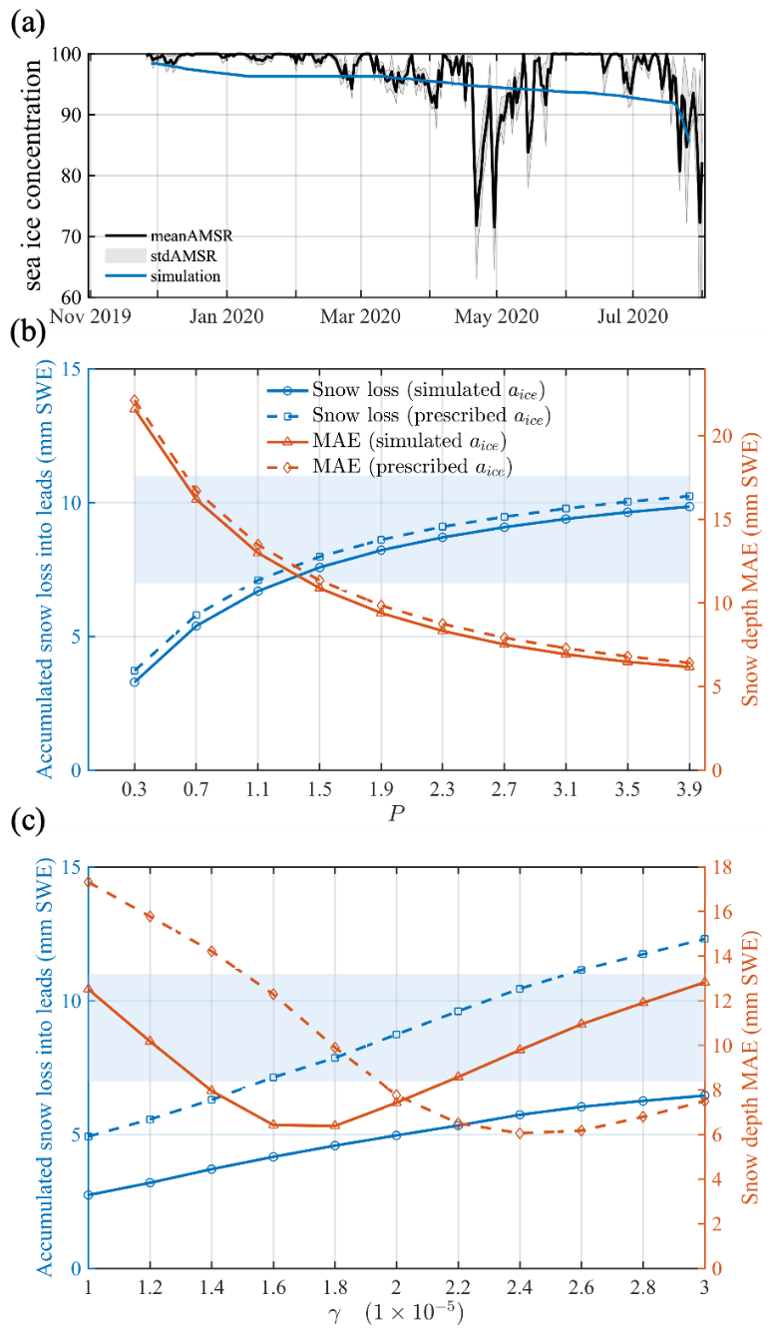
Figure 3 (a) Time series of sea ice concentration from AMSR2 observations and Icepack simulations. (b) and (c) show the statistical results for sensitivity experiments for two snow redistribution parameterizations: bulk redistribution with varying p, and blowing-snow redistribution with varying γ, respectively. The blue line and the left blue y axis represent the accumulated snow loss into open leads during the period from 19–28 April, while the orange line and the right orange y axis indicate the mean absolute error (MAE, in mm SWE) between simulated and observed snow thickness. The blue shaded area denotes the observed range of accumulated snow loss into open leads (∼7–11 mm area-averaged SWE) based on Clemens-Sewall et al. (2023). Solid lines denote simulations with model-simulated sea ice concentration, whereas dashed lines denote simulations with prescribed observed sea ice concentration. a_ice denotes AMSR2 sea ice concentration.

In the snow mass balance, snow thickness is influenced by snowfall (S_f), snowmelt (S_m), snow sublimation (S_su), snow-ice formation (S_i), and snow loss into open leads (S_lo). In reality, snow can also be lost during sea ice ridging when part of the snow cover becomes subducted and submerged; however, this process is not explicitly represented in the Icepack configuration used in this study. This study investigates the impact of different snow redistribution schemes, with and without prescribing sea ice concentration, on the snow mass balance. The results (Fig. 4) show that, compared to the no-redistribution experiment, the bulk scheme increases the amount of snow entering the leads by reducing the snowfall reaching the ice layer. Additionally, model diagnostics indicate enhanced snow-ice formation in the snwITDrdg scheme relative to the bulk scheme. In addition to depositing a portion of snow mass into open leads, the snwITDrdg scheme diagnostically redistributes snow among ice thickness categories. This redistribution, modulated by the ridged-ice fraction and surface type within each category, results in increased snow thickness over thinner ice categories, making the ice more susceptible to surface flooding and subsequent snow-ice formation. However, enhanced snow-ice formation is not evident in the averaged SIMBA observations used in this study. Furthermore, previous studies have suggested that Icepack may overestimate snow-ice formation (Gu et al., 2022). Therefore, this category-dependent redistribution should be interpreted as a model-diagnostic mechanism rather than as a directly validated observational feature.

Compared to the bulk scheme, the bulkm configuration removes a larger fraction of precipitation, resulting in reduced overall snow accumulation. Meanwhile, the snwITDrdgm configuration increases snow loss into leads relative to snwITDrdg, thereby reducing snowmelt at the end of the simulation. The sublimation losses are relatively consistent across all snow redistribution schemes. Prescribing sea ice concentration has minimal effect on the no-redistribution experiment and bulk schemes. However, within the snwITDrdg and snwITDrdgm scheme, prescribing sea ice concentration leads to a significant reduction in snow loss into leads and a corresponding increase in snowmelt. This difference arises because the bulk redistribution scheme primarily reduces incoming snowfall through a prescribed level-ice-dependent fraction, making it less sensitive to changes in sea ice concentration. In contrast, the snwITDrdg scheme redistributes wind-eroded snow into open leads, so its snow-loss term depends more directly on the open-water fraction. Prescribing AMSR2 sea ice concentration therefore modifies the amount of snow lost to leads and changes the remaining snow available for subsequent melt.

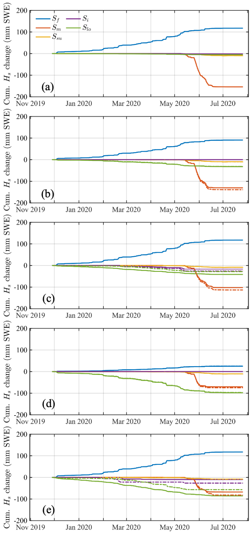
Figure 4 Time series of cumulative snow mass changes in (a) no-redistribution, (b) bulk, (c) snwITDrdg, (d) bulkm and (e) snwITDrdgm redistribution configurations. Different colored lines represent snowfall (S_f), snowmelt (S_m), snow sublimation (S_su), snow-ice formation (S_i), and snow loss into open leads (S_lo), respectively. Solid lines denote simulations without prescribed AMSR2 sea ice concentration, while dashed lines indicate simulations with prescribed AMSR2 sea ice concentration.

4 Discussions

Despite improvements in the optimized bulk redistribution and blowing-snow redistribution configurations, several limitations remain. The simulated snow thickness still peaks approximately 7 d later than observed and melts too quickly in summer. This discrepancy may partly stem from uncertainties in snowfall forcing. Wagner et al. (2022) showed that MOSAiC snowfall estimates differ among products, and we used the PWD–ERA5 average to reduce product-dependent uncertainty. However, event-scale biases in snowfall timing, frequency, or magnitude may remain. For example, between 6 and 13 May, the PWD–ERA5 average shows increased snowfall (Fig. 1c), whereas the observed snow thickness declined. We interpret this mismatch as a possible overestimate of snowfall during this event. However, this discrepancy may also reflect unresolved snow-loss processes, including sublimation of drifting and blowing snow, non-local snow transport, and limitations in the model representation of snow compaction and density evolution. Rapid summer melt may also result from missing melt-pond physics or inaccurate snow thermal conductivity, leading to excessive surface heat fluxes (Yin et al., 2021). In addition, Icepack estimates a constant snow density of 330 kg m⁻³, whereas actual snow density evolves with wind compaction, temperature fluctuations, moisture content, and sublimation (Liston et al., 2020; Macfarlane et al., 2023), contributing to mass and thickness biases. The treatment of suspended snow particles is simplified in Icepack: the fraction of suspended snow that is passed directly to the ocean through leads. While sublimation of suspended snow represents an important loss pathway in the Arctic (Liston et al., 2020; Robinson et al., 2025), it is not explicitly represented in the present model configuration. As a result, the optimized p and γ values should be interpreted as effective parameters that may compensate for multiple unresolved snow-loss processes, including lead trapping, wind-driven redistribution, and blowing-snow sublimation, as well as possible biases in snowfall forcing.

Previous studies have shown that snow accumulation and redistribution vary among different sea-ice regimes because of differences in ice age, ice type, deformation state, and surface roughness (Clemens-Sewall et al., 2022). Field observations have also demonstrated pronounced subgrid-scale spatial variability in snow thickness (Huang et al., 2026; Mallett et al., 2022). However, Icepack assumes a spatially uniform snow thickness within each ice-thickness category and therefore does not explicitly resolve this subgrid-scale heterogeneity, which may introduce uncertainty into the simulated snow distribution and its thermodynamic influence on sea ice. Consequently, the parameter p and the performance of snow redistribution parameterizations may vary under different sea-ice conditions. The observational dataset used in this study includes both first-year ice and second-year ice conditions. However, the limited number of available SIMBA buoy sites does not allow a robust evaluation of individual parameterization schemes for specific ice regimes or subgrid-scale snow variability. Therefore, the evaluation presented here is based on the mean snow thickness over the observational region, and the optimized parameter values and conclusions should be interpreted as representing the average snow redistribution behaviour across the range of sea-ice conditions sampled during MOSAiC. Since the same model assumption is adopted consistently in all simulations, it is unlikely to affect the relative comparison among the snow redistribution parameterizations examined in this study. Future work incorporating more realistic representations of subgrid-scale snow heterogeneity together with expanded observational datasets will help further quantify these uncertainties and improve the representation of snow redistribution processes under different sea-ice conditions.

Our study is complementary to Zhao et al. (2025), who evaluated Icepack simulations along the MOSAiC drift trajectory using no-redistribution, bulk redistribution, and snwITDrdg configurations. Zhao et al. (2025) focused mainly on sea ice thickness and the combined influence of snow redistribution and melt-pond schemes. In contrast, the present study focuses on snow thickness/SWE and the snow mass budget, especially the sensitivity of simulated snow loss to leads to the bulk redistribution parameter p, the blowing-snow erosion coefficient γ, and prescribed AMSR2 sea ice concentration. Therefore, while both studies show that snow redistribution strongly affects Icepack simulations during MOSAiC, our analysis provides a more direct evaluation of snow redistribution parameterizations against MOSAiC snow observations and observed lead-related snow loss. Differences between the results of the two studies likely arise from differences in forcing data, model version and configuration, sea ice concentration treatment, observational constraints, and the specific target variable used for evaluation.

Although the representativeness of the MOSAiC observations should be considered, they constitute one of the most comprehensive datasets for examining snow and sea ice processes in the central Arctic. The findings of this study provide new insights into snow thickness simulation and the parameterization of snow redistribution, contributing to improved modeling of Arctic snow conditions.

5 Conclusions

Snow plays a vital role in sea ice thermodynamics, yet snow accumulation remains a key uncertainty in sea ice modeling. Using the Icepack column model, we simulated snow thickness during the MOSAiC campaign under two snow redistribution parameterizations and multiple model configurations, and further explored both bulk and blowing snow redistribution parameterizations to enhance the agreement with observations. Our results show that without snow redistribution, simulated snow thickness is significantly overestimated in winter and spring. The bulk redistribution scheme slightly reduces snow accumulation, but does not substantially change the timing of the seasonal peak or melt onset. The snwITDrdg redistribution scheme further reduces snow thickness and improves the magnitude of the simulated seasonal evolution, though biases persist, especially during snowfall events and around the seasonal peak.

To address this issue, we conducted sensitivity experiments for both snow redistribution schemes. In the bulk scheme, we varied the parameter p from 0.3 to 4 based on MOSAiC observations. When p=4, the simulated snow thickness shows the best agreement with observations, with a mean absolute error (MAE) of 6.2 mm. In the snwITDrdg scheme, given the large observational uncertainties in snow density and subgrid-scale ice thickness distribution (ITD), the coefficient γ is treated as an effective tuning parameter that accounts for unresolved uncertainties in snow physical properties and ice thickness heterogeneity. We varied γ from $\mathrm{1}\times {\mathrm{10}}^{-\mathrm{5}}$ to $\mathrm{3}\times {\mathrm{10}}^{-\mathrm{5}}$, with and without prescribing AMSR2 sea ice concentration. When sea ice concentration is not prescribed, adjusting γ does not lead to accumulated snow loss to leads within the observed range of 7–11 mm area-averaged SWE. In contrast, when AMSR2 sea ice concentration is prescribed, the simulated accumulated snow loss to leads falls within the observed range. Specifically, when $\mathit{\gamma }=\mathrm{2.4}\times {\mathrm{10}}^{-\mathrm{5}}$, the simulated snow thickness generally agrees well with observations, yielding a mean absolute error of 6.4 mm. These results indicate that the parameter p in the bulk scheme and the effective tuning coefficient γ in the snwITDrdg scheme both have a significant influence on simulated snow thickness. Moreover, accurate sea ice concentration is crucial for realistic snow thickness simulations in the snwITDrdg scheme.