Multi-sensor satellite analysis reveals latitudinal and morphometric controls on ice phenology across 31 000 lakes on the Alaska North Slope

Thermokarst lakes are critical components of Arctic carbon cycling, yet their ice phenology remains poorly characterized at regional scales. We present the first comprehensive analysis of ice-on and ice-off timing across 30 774 lakes on the Alaska North Slope using Sentinel-1 synthetic aperture radar (SAR) classified by a Random Forest (RF) model trained using labels derived from Sentinel-2 optical imagery and ERA5 temperature data for the period 2019–2023. Our RF classifier achieved 94 % accuracy for ice state detection, enabling phenology retrieval for 97 % of lake-years. Results revealed a mean ice-free period of 114 d (standard deviation = 25 d), with ice-off occurring at day-of-year 159 (8 June) and ice-on at day-of-year 273 (30 September). Spatial analysis demonstrated strong latitudinal control on ice phenology, with ice-free duration decreasing by 23 d per degree northward. Lake morphology (area, circularity, convexity, and shoreline development index) showed modest but significant effects on ice timing after controlling for latitude effects, with shoreline development index and convexity each contributing ∼ 3 d variation across typical lake ranges. Comparison of the RF model and simplistic accumulated degree-day (ADD) model-detected ice phenology yielded a convincing match, where the offsets in ice phenology between the models fell within twice the per-detection observation gap for approximately 80 % of the lakes. Furthermore, these offsets exhibited the same strong latitudinal control and negligible effects of lake morphology. These lake-specific phenology dates provide timing and duration constraints for future methane studies using high-resolution sensors and provide baseline phenology data essential for understanding how continued Arctic warming will affect thermokarst lake dynamics and associated carbon cycle feedbacks.

1 Introduction

The Arctic is warming at nearly two to four times the global average rate (Rantanen et al., 2022), with profound implications for thaw on permafrost landscapes. This Arctic Amplification (Serreze and Barry, 2011) impacts Arctic landscapes through processes such as the permafrost carbon feedback (Schuur et al., 2015), alteration of surface hydrology (Lafrenière and Lamoureux, 2019), landscape changes (Bryant et al., 2025) and ground subsidence (Streletskiy et al., 2025). Formed by ground subsidence following permafrost thaw, thermokarst lakes cover more than 20 % of the Alaskan Arctic Coastal Plain (Arp et al., 2011) and approximately 17 % of Arctic lowland terrain globally (Muster et al., 2017). The majority of North Slope lakes are thermokarst in origin (Farquharson et al., 2016; Jones et al., 2022), with aeolian processes also playing an important role in lake origin and thermokarst lake evolution and orientation (Carson and Hussey, 1962). Additionally, glacial processes are another likely source of lake origin, specifically in the foothills of the Brooks Range (Detterman et al., 1958).

Thermokarst lakes represent dynamic components of high-latitude carbon cycling, where permafrost thaw surrounding these lakes mobilizes stored soil organic material (in 't Zandt et al., 2020). These lakes emit substantial quantities of methane (CH₄) and carbon dioxide (CO₂) to the atmosphere (Walter Anthony et al., 2018), where current estimates for yearly CH₄ emissions from thermokarst lakes larger than 0.1 km² are 24.0 ± 8.4 Tg CH₄ yr⁻¹ (Zhuang et al., 2023). Emissions are strongly modulated by lake area and depth (Heslop et al., 2020; Manasypov et al., 2023; Matthews et al., 2020; West et al., 2016) and the duration of ice melt and seasonal ice cover (Mu et al., 2025; Wik et al., 2016; Guo et al., 2020). However, the influence of lake morphometrics on ice condition and timing (i.e., duration of ice melt and seasonal ice cover) is relatively understudied.

Ice phenology – the timing of ice formation (ice-on) and breakup (ice-off) – controls the duration of open-water conditions during which gas exchange with the atmosphere occurs. Despite the importance of ice timing for understanding carbon fluxes, comprehensive regional-scale phenology data remain scarce at high spatiotemporal resolution (< 0.25 km px⁻¹ per week) (Matthews et al., 2020). Previous studies have either focused on direct observation of ice phenology for individual lakes using in situ observations (Arp et al., 2015) or use single-sensor/single-modality satellite approaches for lake populations with a relatively limited number of lakes (< 1000; Latifovic and Pouliot, 2007; Surdu et al., 2014, 2016; Tom et al., 2020). The challenge of monitoring hundreds of thousands of thermokarst lakes across the remote Arctic terrain, combined with persistent cloud cover and polar night conditions, has hindered systematic phenology characterization. This technical challenge limits our ability to resolve the timing and duration of freeze-thaw transitions and detect climate-driven shifts in ice phenology, constraining efforts to quantify lake-atmosphere carbon exchange and accurately represent thermokarst lake processes in regional and global Earth system models.

Current direct methods for constraining lake ice phenology typically utilize simplistic thermal diffusion metrics such as the modified Stefan equation for accumulating degree days (ADD) (°C × days; Arp et al., 2015; Stefan, 1890). ADD metrics are determined from air temperature records and do not account for lake-specific morphology (USACE, 2004). More complex models may incorporate lake depth, which captures ice thickness, but do not generally account for other morphologic parameters such as area, circularity, convexity, or shoreline properties, as these features are difficult to estimate without in situ measurements (Duguay et al., 2003). As a result, the degree to which thermokarst lake morphology may influence ice phenology relative to estimates based on ADD metrics, which do not account for morphology, remains largely unknown. Previous studies suggest that lake morphology, especially area and depth, play an important role in modulating ice phenology (Basu et al., 2024; Higgins et al., 2021; Smits et al., 2021). Specifically, the relationship between lake depth and ice thickness – which dictates whether lake ice is bedfast or floating – exerts a strong control on ice-off timing, occurring on average 17 d earlier for bedfast ice lakes than floating ice lakes in Northern Alaska (Arp et al., 2015). Recent advances in satellite remote sensing offer new opportunities for large-scale ice monitoring (Bartsch et al., 2023). The Sentinel-1 synthetic aperture radar (SAR) operates independently of solar illumination and cloud cover, providing year-round observations at ∼ 10–20 m spatial resolution. The distinct microwave radar backscatter signatures of ice versus open water enable automated ice detection for thermokarst lakes (Bartsch et al., 2017; Tom et al., 2020), though interpretation can be complicated by factors including ice thickness and structure, snow cover, bulk water content, and surface roughness that all impact radar scattering properties (Hall et al., 1994; Jeffries et al., 1994). However, Sentinel-2 optical imagery provides complementary information through spectral indices such as the Normalized Difference Snow Index (NDSI), which discriminates ice from water under sun-lit, clear-sky conditions (Riggs et al., 2017). NDSI can aid in SAR interpretation and fill in dates within the Sentinel-1 6 d repeat time when using both polar orbiting ascending and descending tracks. By combining these observations with temperature data from atmospheric reanalysis products, robust ice classification can be achieved across the full annual cycle, allowing for a regional-scale exploration of the morphologic controls on lake ice phenology.

In this contribution, we present a multi-sensor fusion approach to characterize ice phenology and its relationship to morphological parameters across 30 774 thermokarst lakes on the Alaska North Slope. Our objectives are to: (1) develop and validate an automated ice detection algorithm combining SAR, optical, and temperature data; (2) quantify spatiotemporal patterns in ice-on and ice-off timing across the study region relative to ADD-predicted timing; (3) examine relationships between lake morphometry and ice phenology. This analysis provides the most comprehensive characterization of regional-scale thermokarst lake ice phenology to date, establishing baseline conditions against which future changes can be assessed.

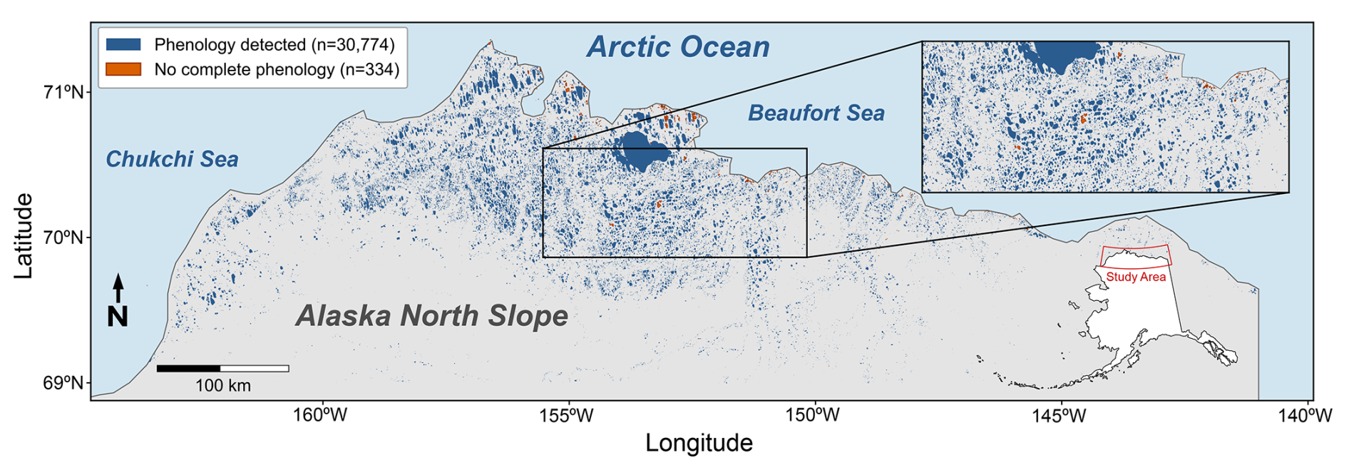
Figure 1 Study area (69–71.36° N, 163.85–141.02° W) showing the 31 108 lakes with area ≥ 0.02 km² selected for analysis, of which 30 774 (blue) yielded ice phenology. Lakes for which phenology was not successfully detected are shown in bronze. Inset depicts lake details within the study region. Sources: ALPOD and the Natural Earth.

2 Methods

2.1 Study area and lake dataset

The study area encompasses the Arctic Coastal Plain (ACP) of the North Slope of Alaska (∼ 69–71.36° N), a ∼ 200 000 km² region of continuous permafrost extending from the Brooks Range foothills to the Arctic Ocean (Fig. 1). This low-relief coastal plain is characterized by hundreds of thousands of 2–4 m deep thermokarst lakes formed in ice-rich permafrost deposits (Hinkel et al., 2012). The region experiences a polar climate with mean annual temperatures of −10 to −12 °C, though summer temperatures regularly exceed 15 °C.

We obtained lake boundaries from the Alaska Lake and Pond Occurrence Dataset (ALPOD; Levenson et al., 2025), which provides high-resolution (10 m px⁻¹) lake polygons derived from a U-Net lake detection model (Mullen et al., 2023) applied to multi-temporal Sentinel-2 imagery across Alaska that totals in 801 895 lakes. The selected study region (69-71.36° N, 163.85–141.02° W) contains 128 197 ALPOD lakes. We selected all lakes ≥ 0.02 km² (2 ha) to ensure each lake had a large enough number of pixels (200 for 10 m px⁻¹ imagery) for reliable Sentinel-1/2 detection. This selection yielded 31 108 total lakes for analysis, which encompasses the upper ∼ 25th percentile of lake area distribution prior to area filtering (Fig. S10 in the Supplement). From this, we were able to retrieve phenology from 30 774 lakes (98.9 %), where lake morphometrics could be extracted using lake polygons from the ALPOD database.

For the subpopulation of lakes used in this study, lake area spans five orders of magnitude from 0.02 to 859 km² (median = 0.065 km²), with the upper bound corresponding to Teshekpuk Lake. Study lakes had a range of circularity, defined as C = $\mathrm{4}\mathit{\pi }A/P^{\mathrm{2}}$, where P is lake perimeter (m), from 0.01–0.78, with smaller values indicative of more oblong lakes. Lake shoreline development indices, (SDI = $P/\mathrm{2}\sqrt{\mathit{\pi }A}$; Hutchinson, 1957), which quantifies shoreline complexity, range from 1.13–10.02, with larger values indicating more complex shorelines. Measures of lake convexity range from 0.11–0.998, where values of 1.0 indicate more convex shorelines and values closer to zero signify higher concavity or shoreline irregularity (Bozeman and Pilling, 2013). Calculating both SDI and convexity allows for a better understanding of both shoreline complexity and irregularity, where SDI is more impacted by fractal dimensionality from higher resolution data and increases with increasing area of lakes (Seekell et al., 2022). Lake circularity, convexity, and SDI for the subpopulation of lakes used in this study were consistent with metrics from the full ALPOD database (Fig. S10).

2.2 Satellite data acquisition and preprocessing

We acquired Sentinel-1 Ground Range Detected (GRD) imagery from Google Earth Engine (GEE) (Gorelick et al., 2017) for the period January 2019 through December 2023. We selected this time scale based on the availability of the Harmonized Sentinel-2 MSI: MultiSpectral Instrument, Level-2A (SR) collection from Google Earth Engine. 2019 was selected as the start year, as the 2017–2018 data does not have global coverage in this collection. Using 2023 as the final year for this data date range ensured that there were at least five years of data to retrieve lake ice phenology from, where we sought to define a nominal five-year time span over which to perform this analysis. The loss of Sentinel-1B on 23 December 2021, affected our analysis in increasing the repeat time (from 6 to 12 d) between acquisitions over our study area, thereby effectively decreasing the density of measurements after data transmission failure of the satellite.

We used images from both ascending and descending track satellite orbits acquired in Interferometric Wide Swath mode, providing both vertical transmit/receive (VV) and vertical transmit/horizontal receive (VH) polarizations at 10 m resolution. Images were accessed from the GEE Sentinel-1 GRD collection, which provides data pre-processed using the standard Sentinel-1 Toolbox workflow including thermal noise removal, radiometric calibration, and orthorectification terrain correction (Mullissa et al., 2021). We additionally applied an incidence angle mask (25–50°) to reduce edge effects, and we subtracted VH from VV images to generate $\mathrm{VV}/\mathrm{VH}$ images. We generated standard falsecolor RGB composites of backscatter (i.e., red: VV, green: VH, blue: $\mathrm{VV}/\mathrm{VH}$) (see Fig. S1 in the Supplement for the entire workflow). To account for typical Arctic lake backscatter ranges, we scaled each band (in order) for open water to rough ice (−20 to −5 dB; VV), volumetric scattering cross-polarization range (−28 to −12 dB; VH), and the polarization ratio (8 to 18 dB; $\mathrm{VV}/\mathrm{VH}$). We scaled each band to target specific dB ranges that aid in differentiation between ice and water as well as potential ice type/thickness. By scaling the data, we target these specific dynamic ranges to maximize differentiation between the expected minimum and maximum expected backscatter values for the ice/water distinction for a given band. Additionally, scaling the data reduces the impact of extraneous outliers outside of the expected backscatter ranges for each band (Surdu et al., 2015; Murfitt and Duguay, 2020).

We obtained Sentinel-2 Level-2A surface reflectance imagery for the same time period between 2019–2023, where our study period date range is limited by Sentinel-2 Level-2A products being unavailable for 2017–2018. We then filtered to acquisitions with < 80 % scene cloud cover and pixel-level cloud and cloud shadow masking using the s2cloudless algorithm with a 20 % cloud probability threshold (Sentinel-Hub, 2025; Skakun et al., 2022). Sentinel-2 coverage varies spatially across the study area due to orbital geometry at ∼ 70° N, with reduced coverage between 153 and 157° W longitude; consequently, S2 observations serve as high-confidence training labels where available rather than as the primary detection method. We calculated the Normalized Difference Snow Index (NDSI) as NDSI = (Green − SWIR) $/$ (Green + SWIR) using bands B3 (560 nm) and B11 (1610 nm) (Hall et al., 1995), and we classified NDSI values > 0.4 as snow/ice following established thresholds (Riggs et al., 2017). The output of the NDSI is a binarized classification that is later used to calculate ice fraction, as explained in Sect. 2.3.

We obtained ERA5 hourly 2 m air temperature data at 0.25° (∼ 28 km px⁻¹) resolution from the Google Cloud Analysis-Ready, Cloud-Optimized (ARCO) ERA5 archive (Carver and Merose, 2023; Hersbach et al., 2017, 2020) and aggregated to daily means for each lake centroid location. Prior work has demonstrated excellent agreement between ERA5 and in situ weather stations across the Arctic (Clelland et al., 2024; Ibebuchi et al., 2024; Tarek et al., 2020; Pernov et al., 2024). For example, Clelland et al. (2024) has shown agreeance of ERA5 with in-situ data in Siberia, Ibebuchi et al. (2024) find ERA5 outperforms other reanalysis products for comparison with in-situ data across the contiguous United States, Tarek et al. (2020) found ERA5 hydrological modeling was comparable to in-situ data across North America, and Pernov et al. (2024) found a 0.94 R² for temperature when comparing ERA5 to 17 weather stations across the Arctic. Given the agreement of prior work of validating ERA5 in the Arctic, we use ERA5 2 m air temperature data for this study over the ACP.

2.3 Ice detection algorithm

Our ice detection approach uses a Random Forest (RF) classifier (Breiman, 2001) to predict ice state from Sentinel-1 SAR backscatter features. This approach follows machine learning methods developed for lake ice classification from SAR imagery (Hoekstra et al., 2020; Tom et al., 2020), adapted for regional-scale application. Due to variations in liquid water content, and therefore dielectric permittivity and radar backscatter (Unterschultz et al., 2009), during phase changes, it is particularly difficult to classify SAR imagery for phenology during the shoulder season (Posch et al., 2024). To mitigate the effects of these factors on ice detection, we introduce a series of temperature-based thresholds, consistency checks, and consecutive occurrences. First, we derived training labels from two sources: ERA5 temperature reanalysis and Sentinel-2 optical imagery. Sustained temperature periods (10+ consecutive days below −20 °C or above +10 °C) provided high-confidence labels during winter months and polar night when optical data were unavailable, comprising approximately 62 % of training labels. Sentinel-2 NDSI classifications provided the remaining labels during cloud-free conditions (30 % cloud threshold), with temperature-based quality control to exclude potentially erroneous detections (e.g., S2 labels flagged as water when air temperature was below −5 °C, or as ice when temperature exceeded +5 °C, were excluded to filter algal bloom misclassifications). This dual-source approach maximizes temporal coverage across the full annual cycle while maintaining label reliability.

We trained the RF model on six Sentinel-1-derived features: VV and VH backscatter (dB) measured over the lake interior (extracted from removing a 10 m interior buffer applied to each lake feature perimeter), VV and VH backscatter over a 100 m marginal landscape surrounding each lake (extracted from adding a 100 m exterior buffer applied to each lake feature perimeter), and the $\mathrm{VV}/\mathrm{VH}$ polarization ratio for both lake and landscape zones. The classifier was trained using mean ice fraction values (0–1) from both the interior and exterior lake buffers, applied to the Sentinel-2 NDSI-derived ice labels and the corresponding Sentinel-1 training data. A given lake-date is labeled as either ice or water using a threshold of ice fraction > 80 % being ice, and an ice fraction < 20 % being water. As a result, the approach does not explicitly capture spatial variations in ice growth or melt within a lake, except to the degree that they are reflected in the buffer-averaged values. High values of VV co-polarization record rough ice, whereas low values record smooth ice and water. VH cross-polarization is sensitive to volumetric scattering from vegetation, and the ratio between co- and cross-polarizations aids in determination between types of ice. Furthermore, the landscape features encapsulated through the exterior buffer capture contextual information about surrounding terrain conditions that may aid in distinguishing ice from open water (e.g., freeze/thaw state of the landscape).

Training data comprised 1.09 million lake-date observations from 24 886 lakes. An additional 274 079 observations from 6222 held-out (validation) lakes were reserved for testing. This lake-based splitting strategy, implemented using grouped cross-validation, ensures no lake appears in both training and test sets, preventing data leakage from temporal autocorrelation within individual lake time series. We implemented the RF model using scikit-learn (Pedregosa et al., 2011) with 100 trees, a maximum depth of 15, a minimum split of 20 samples, and a minimum of 10 samples for leaves.

2.4 Phenology extraction

Using the RF model predictions, we output the probability that an individual lake-date is covered with ice, P(ice). We determined the ice-on and ice-off dates from this classified ice probability time series, P(ice), for each lake-year. To avoid detecting spurious mid-winter thaws or brief summer re-freezing events, we constrained transition detection using hysteresis logic, where a lake-date with P(ice) > 0.7 was labeled as ice and P(ice) < 0.3 as water. Lake-dates that have P(ice) greater than 0.3 but less than 0.7 are determined ambiguous.

We then use the date prior to transition with the first date post-transition to interpolate the day in which the bimodally-distributed P(ice) crosses 0.5 (as determined by the symmetric distribution around the consistently global trough at 0.5). To prevent logical inconsistencies in the detected phenology (e.g. negative ice free and ice-covered periods), we only defined ice-off if it started and is observed for a given year. This is implemented in the case that ice-off for an individual lake may have been detected as open throughout the prior winter season, where we remove that given lake-year's phenology for the current year's ice-off. Functionally, ice-off is the first date when the lake transitioned from frozen to open water state and remained classified as water for at least two consecutive observations and satisfies the imposed hysteresis logic. Similarly, we defined ice-on for a lake as long as it started and is observed for a given year. Otherwise, the lake will have frozen into the next year's late winter/early spring outside of that given year. In such cases, as for ice-off, we remove and exclude that lake-year's relevant phenological event. Likewise, ice-on is the first date of the subsequent freeze-up when the lake transitioned to frozen state and remained classified as ice for at least two consecutive observations. With both ascending and descending Sentinel-1 orbits providing a median observation gap of 4 d at this latitude, this criterion typically requires sustained state persistence of approximately 8–16 d, filtering transient events while preserving sensitivity to true phenological transitions.

We then calculated the ice-free period as the number of days between ice-off and ice-on for each lake-year. We assigned null values to lakes lacking clear transitions due to data gaps, persistent cloud cover, or ambiguous classifications and excluded them from phenology statistics. We computed summary statistics including mean, median, standard deviation, and interquartile range across all valid lake-years, as well as stratified by geographic subregion and lake size class.

2.5 Phenology model comparison

To compare the SAR RF model with other methods for ice phenological timings, we used ERA5 daily average 2 m temperatures (Carver and Merose, 2023; Hersbach et al., 2017; Hersbach et al., 2020) to calculate a continuous time series of both the accumulated degree day of thaw (ADDT) and accumulated degree day of freezing (ADDF) for ice thickness (Arp et al., 2015; Stefan, 1890).Accumulated Degree Days of Thaw (ADDT) and Accumulated Degree Days of Freeze (ADDF) were calculated from daily mean air temperatures (T_i) on day i as cumulative sums of positive and negative temperatures, using Eqs. (1) and (2), respectively:

$$\begin{array}{}\text{(1)}& {\displaystyle }& {\displaystyle }\text{ADDT}=\sum _{i=\mathrm{1}}^n\left\{\begin{array}{c}{T}_i,T_i>\mathrm{0}\\ \mathrm{0},T_i\le \mathrm{0}\end{array}\right\}\text{(2)}& {\displaystyle }& {\displaystyle }\text{ADDF}=\sum _{i=\mathrm{1}}^n\left\{\begin{array}{c}-T_i,T_i<\mathrm{0}\\ \mathrm{0},T_i\ge \mathrm{0}\end{array}\right\}\end{array}$$

We calculated both of these metrics for each lake-year combination and used a seven-day switch window between freeze-thaw/thaw-freeze to ensure a sufficient duration for cumulative ice growth/melt before switching between ADDF and ADDT. We then converted from the accumulating degree days of freeze to ice thickness, h_ice (cm), using Eq. (3):

$$\begin{array}{}\text{(3)}& h_{\text{ice}}=\mathit{\alpha }\sqrt{\text{ADDF}}\end{array}$$

Where α is the Stefan equation coefficient, with a chosen value of 2. During the seven-day switch window, ice thickness was estimated using Eq. (4):

$$\begin{array}{}\text{(4)}& h_{\text{ice}}=\mathit{\alpha }(\sqrt{\text{ADDF}}-\sqrt{\text{ADDT}})\end{array}$$

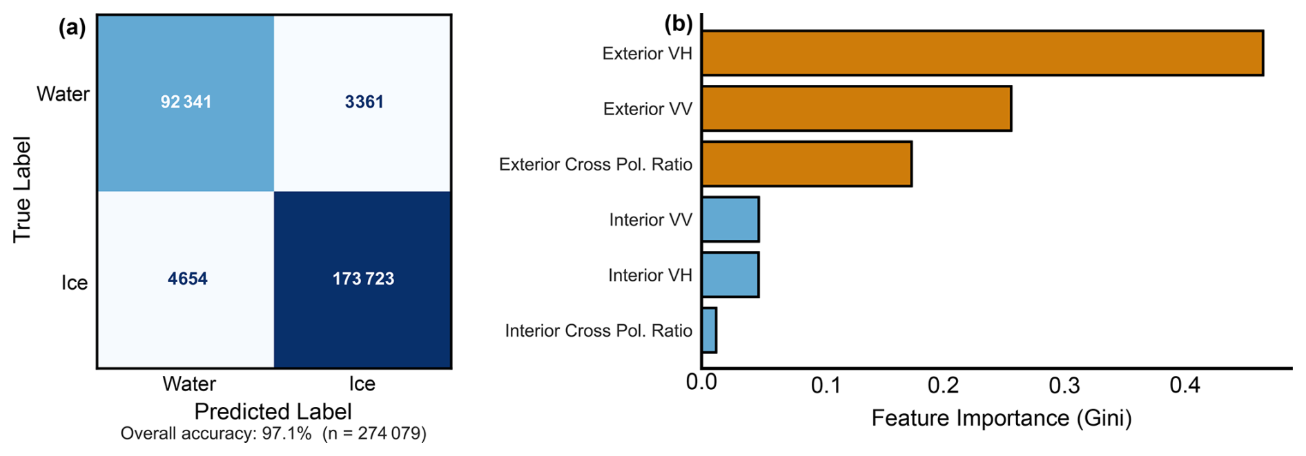
Figure 2 (a) Random forest classification confusion matrix, where numbers within each box represent number of samples falling within each category. The boxes with darker saturation indicate where the RF model predicted the correct label based on the true label, where correct water and ice predictions are represented by medium blue and dark blue, respectively. The light blue/gray boxes indicate where the RF model predicted incorrectly. (b) Random forest feature importance using Gini, where land and lake refer to the exterior and interior lake buffers, respectively. VV, VH, and $\mathrm{VV}/\mathrm{VH}$ ratio refer to the polarimetric SAR band, and db represents decibels.

During the seven-day switch, ice thickness values were used if positive, if h_ice≤0, ice thickness was set to zero to avoid negative ice thicknesses. For similar reasons, ice thickness was set to 0 for the ADDT period. We utilize this method because ADD metrics only require daily air temperatures and the empirically derived α coefficient. This approach is advantageous across our large study where many of the variables utilized in more complex thermodynamic models are simply unavailable or poorly constrained given the limited in-situ data that exists across the North Slope. This method also allows us to capture first order patterns while remaining computationally efficient, which is the primary objective of this study. Consequently, the model provides robust first-order estimates of spatial and temporal variability in ice thickness while avoiding the substantial uncertainties associated with poorly constrained thermodynamic parameters. For inter-model comparison, we used the SAR ice-off and ice-on dates from the transition-based detection described in Sect. 2.4, and defined the ADD thaw and freeze onsets as the start and end of the longest contiguous thawing interval of each year (the principal warm season). Because neither estimate relies on a fixed calendar window, the SAR–ADD comparison is independent of the SAR detection method. We then computed the offsets between the SAR and ADD models by subtracting the ADD from the SAR dates, where positive offsets indicate the SAR model predicting later than the ADD model and vice versa. Finally, we employ the Kruskal–Wallis H-test, Mann–Whitney U-test, and Cliff's Delta (δ) to statistically evaluate any potential controls of latitude and lake morphometry on discrepancies with the RF model and ADD model estimates of ice-off and ice-off dates

3 Results

3.1 Random-forest-derived ice phenology across the Arctic Coastal Plain

The RF classifier achieved 94 % overall accuracy when evaluated against Sentinel-2 NDSI labels from the held-out/validation lakes not used in training (n = 106 527 observations from 2322 lakes). Performance was higher for the ice class (precision = 0.97 recall = 0.95) than the water class (precision = 0.86, recall = 0.93), reflecting both the class imbalance in training data (65 % ice, 35 % water owing to the shorter ice-free season) and the greater difficulty of detecting open water conditions (Fig. 2a). The cross-validated F1 score was 0.977 ± 0.001. Feature importance for the RF model was consistently higher for the land buffers surrounding the lakes for VH (green), VV (red), and $\mathrm{VV}/\mathrm{VH}$ ratio (blue), respectively, compared to the lake interiors (VV, VH, and $\mathrm{VV}/\mathrm{VH}$ ratio), which may indicate true importance or potential bias in the number of pixels used in the land vs lake buffers (Fig. 2b). Accuracy estimates reflect agreement with optical classifications; no independent validation against field observations was performed. During inference, ice state is determined solely by the RF classifier applied to Sentinel-1 features; temperature is not used as a classification input, preserving independence for subsequent analysis of temperature-phenology relationships.

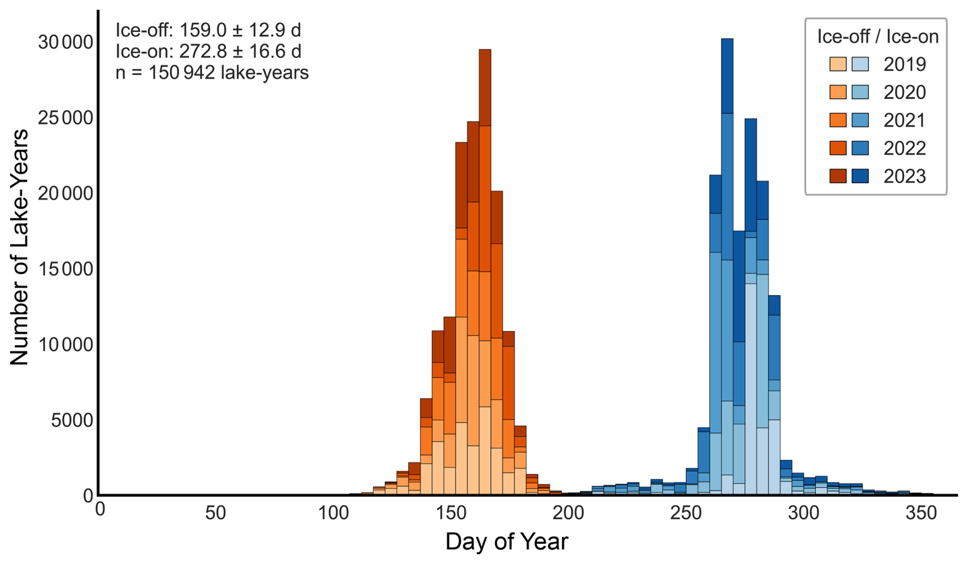
Figure 3 Distribution of SAR RF model-detected ice phenology metrics across all lake-years (2019–2023), where increasing saturation corresponds to more-recent years. The red histogram indicates ice-off date, and the blue histogram indicates ice-on date.

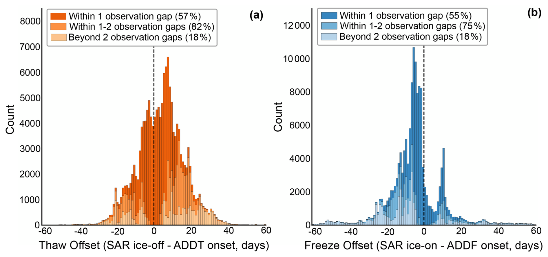
Figure 4 Histograms of the offset between ice phenology timings from SAR detection and the ADDT (a) and ADDF (b) algorithm. Negative values indicate SAR detects dates before ADDT/F, while positive values indicate SAR detects dates after the ADD metric. The histograms are shaded by the per-detection observation gap (i.e., % within 1 observation gap, within 2 observation gaps), where increasing saturation indicates data within shorter periods. The dashed vertical line is at zero which indicates where there is zero offset between the SAR and ADD phenology.

Ice phenology was successfully retrieved for 30 774 lakes (98.9 % of the study population) for at least one year, with 94.17 % having complete five-year records. For the 1.1 % of lakes that do not have detected phenology for at least one year, their overall area probability density distribution and median exhibit no discernible difference between the total population beyond the large difference in the number of samples (Fig. S12 in the Supplement). However, the probability density of SDI and convexity for these lakes without phenology have a medium degree of separability (Cohen's d of 0.57 and 0.52, respectively) compared to the total population (Fig. S12). Furthermore, the lakes without phenology have a higher median SDI value of 2.1 compared to the total lake population of 1.68 which indicates the lakes lacking phenology estimates are comparatively more complex. Across all lakes and years, mean ice-off occurred on day-of-year (DOY) 159 (8 June; standard deviation = 13 d), where the 2σ range is DOY 132 to DOY 185. Mean ice-on occurred on DOY 273 (30 September; standard deviation = 17 d), where the 2σ range is DOY 237 to DOY 308. The resulting ice-free period averaged 114 d (standard deviation = 25 d), with individual lake-years spanning 3 to 331 d (Fig. S2 in the Supplement). Interannual variability in ice timing was substantial (Figs. 3 and S3 in the Supplement). The earliest regional mean ice-off occurred in 2019 (DOY 157), while the latest occurred in 2022 (DOY 164) (Fig. S4 in the Supplement). Likewise, the earliest regional mean ice-on occurred in 2021 (DOY 266), while the latest occurred in 2019 (DOY 278). Ice-free duration ranged from a mean of 105 d in 2022 to 122 d in 2019 (Fig. S4). Across all lake-years, ice-off and ice-on timing were moderately negatively correlated (r = −0.49) across complete paired lake-dates (n = 150 942), largely reflecting latitudinal gradients in both variables (Fig. 5).

Comparison of the ice phenology events derived from the RF model with the ADD metric shows relatively strong correspondence (Fig. 4). There were an identical number of detections valid for comparison for both thaw and freeze. Likewise, the median gap between phenology derived from the RF model and ADD metric was the same at roughly 10 d, varying spatially and after the loss of Sentinel-1B. For ice-off dates, 82 % of lakes align with ADD estimates within twice the per-detection observation gap, and for ice-on dates, 75 % of lakes align within twice the observation gap (roughly 12 d, but varying spatially and after loss of Sentinel-1 B) (Fig. 4). The median gap between the SAR detected ice-on or ice–off date and corresponding ADD metric was 4 d for thaws and 6 d for freezes (Fig. S5 in the Supplement). For ice-off dates, the RF model was earlier than the ADD estimate for 37 % of the lake-years, later than the ADD estimate for 60 % of the lake-years and selected within 6 d for 40 % of the lake-years, suggesting a modest tendency toward delayed thaw detection relative to cumulative degree-day predictions (Fig. S7 in the Supplement). For ice-on dates, the RF model was earlier than the ADD estimate for 77 % of the lake-years, later than the ADD estimate for 21 % of lake-years and selected within 6 d for 38 % of lake-years, reflecting predominately earlier calls from the SAR model during lake freeze-up compared to the ADD model (Fig. S7). See Fig. S13 in the Supplement for a visual representation of the SAR RF model ice phenology performance of a randomly-selected lake.

For all lake-years, for ice-off dates, although statistically significant differences exist in lake morphometrics between cases where the RF model was earlier versus later than the ADD metric (H- and U-test p ≪ 0.05), the effect sizes are very small (δ < 0.15). This indicates that lake morphology does not play a significant role in explaining the observed offset between RF and ADD ice-off estimates. In contrast, latitude has a more significant effect size (H- and U-test p ≪ 0.05; δ = −0.3105), indicating that latitudinal effects likely explain some of the observed mismatch between RF and ADD ice-off timing. Lakes that the RF model identifies as ice-free earlier than the ADD estimate are generally found at lower latitudes while lakes where the RF model identifies the ice-free date later than the ADD estimate are generally located at higher latitudes. Similarly, for ice-on dates across all lake-years, morphology again exhibits statistically significant differences between groups, but with very weak effect sizes (H- and U-test p ≪ 0.05; δ < 0.15), while latitude has a stronger effect (δ = 0.557).

Lakes identified by the RF model as ice-on earlier than the ADD estimate occur at higher latitudes, whereas those identified as ice-on later tend to lie farther south within the study region. Consistently, lakes classified as ice-on earlier by the RF model are substantially farther north than lakes classified as ice-off earlier (δ = −0.3164), and lakes classified as ice-on later are located at higher latitudes than lakes classified as ice-off later (δ = 0.5517).

For lake-years where the offset between the RF model ice-on and ice-off dates and the ADD estimates is greater than 2 revisit gaps, the results are very similar. Within ice-off and ice-on dates, and comparisons between the two dates, morphometrics variables feature statistically significant differences between the groups but weak effect sizes (H- and U-test p ≪ 0.05; δ < 0.18) for differences between the RF model and ADD estimate dates. Latitude, however, continues to be an important variable for offsets between the RF model and ADD estimates. Within ice-off dates, the latitudinal statistical significance and large effect size between groups (H- and U-test p ≪ 0.05; δ = −0.5687) indicates that the RF model selects ice-off dates earlier than the ADD estimates at lower latitudes while selecting ice-off dates later than ADD estimates at higher latitudes. For ice-on dates, the RF model detects ice later than the ADD estimates (δ = 0.6378) at lower latitudes and detects ice earlier than the ADD estimates at higher latitudes. Lakes where the RF detects ice-off earlier than the ADD estimates occur at lower latitudes (δ = −0.5182) while lakes where the RF model detects ice-on earlier than the ADD occur at higher latitudes. Lakes where the RF detects ice-off later than the ADD estimates occur at higher latitudes (δ = 0.6813) and lakes where the RF model detects ice-on later than the ADD estimates occur at lower latitudes.

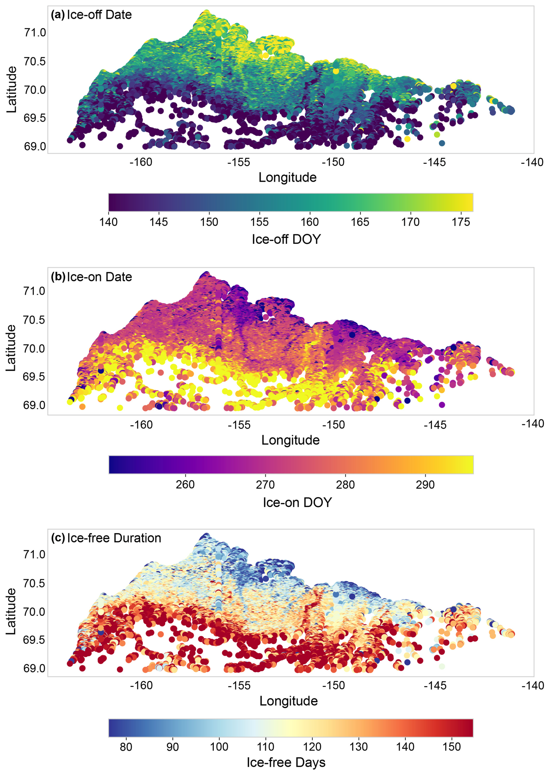
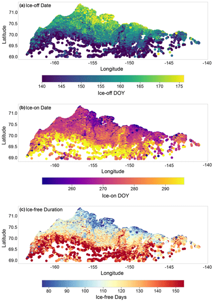
Figure 5 Spatial patterns in mean SAR RF model-detected ice phenology (2019–2023): (a) ice-off date (day of year), (b) ice-on date, and (c) ice-free duration. Each point represents one lake.

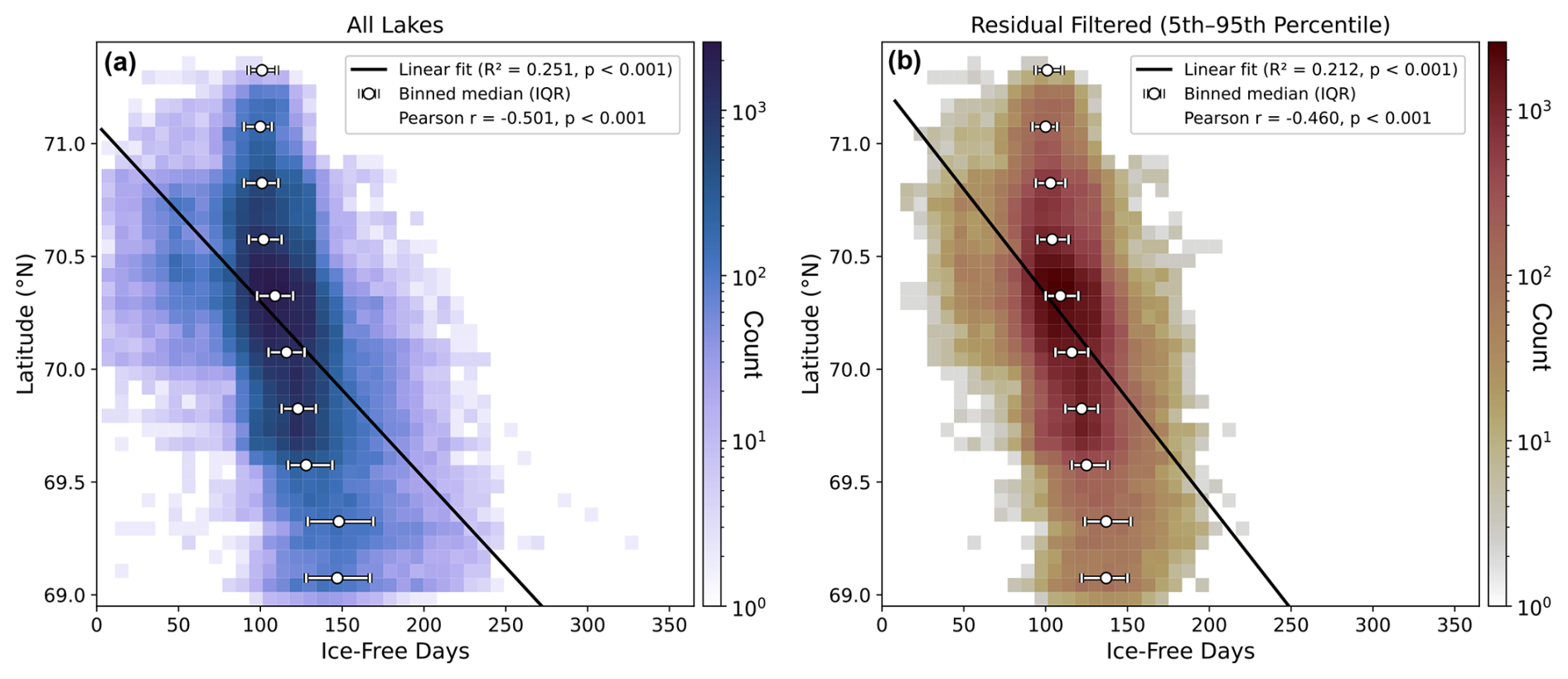
Figure 6 Relationship between latitude and ice-free duration, as determined by the SAR RF model. The black line shows the linear regression best-fit on the raw data. White circles mark the median ice-free days within 0.25° latitude bins, and horizontal bars show the interquartile range (25th–75th percentile); bins with fewer than 30 observations are omitted. Shading shows the number of lake-year observations in each cell of a 40 × 40 grid spanning the range of ice-free days and latitude. (a) All lakes for which phenology was extracted and (b) all lakes with residuals in the 5th–95th percentile. Latitude is displayed on the y-axis for a map view of ice-free duration and is the independent variable in this regression.

3.2 Spatial patterns and latitudinal gradients in lake phenology

Ice phenology exhibited strong spatial structure across the study region (Fig. 5). Latitude was a dominant control on ice timing, with ice-free period decreasing by roughly 30 d per degree northward across all lakes (r = −0.50, p < 0.001; Figs. 5c and 6a); after excluding lakes with residuals outside the 5th–95th percentile, this gradient is 23 d per degree (r = −0.46; see below). This gradient reflects the combined effects of decreasing summer temperatures and shorter warm seasons with increasing latitude. Latitude correlations were strongest for ice-off timing (r = 0.52) and ice-free duration (r = −0.50), and weaker for ice-on timing (r = −0.36) (Fig. S10). Diagnostic tests indicated significant residual spatial autocorrelation (Moran's I = 0.35–0.45) reflecting unmeasured spatially-varying factors such as elevation, microclimate, permafrost properties, surface/subsurface hydrology, and topographic shading (Fig. S6a in the Supplement). Spatial Error Models (SEM) were therefore fit using generalized moments estimation with K-nearest neighbour spatial weights (k=8). The spatial error parameter λ≈ 0.59–0.66 confirmed strong spatial autocorrelation from unmeasured regional factors, and filtered residuals showed negligible spatial autocorrelation (Moran's I ≈ −0.004 to −0.02), indicating adequate model specification (Fig. S6b). Further, the residuals feature a unimodal normal distribution centered around 0, with no additional peak present for lakes in the foothills of the Brooks Range (Fig. 5c). Nonetheless, we also exclude all lakes with residuals outside of the 5th–95th percentile in our analysis, which serves to remove residuals greater than 35 d primarily found in the foothills of the Brooks Range (Fig. S6d). Latitude remains a key control on ice timing even after this exclusion, with the ice-free period decreasing by 23 d per degree northward (r = −0.46, p < 0.001; Fig. 5b).

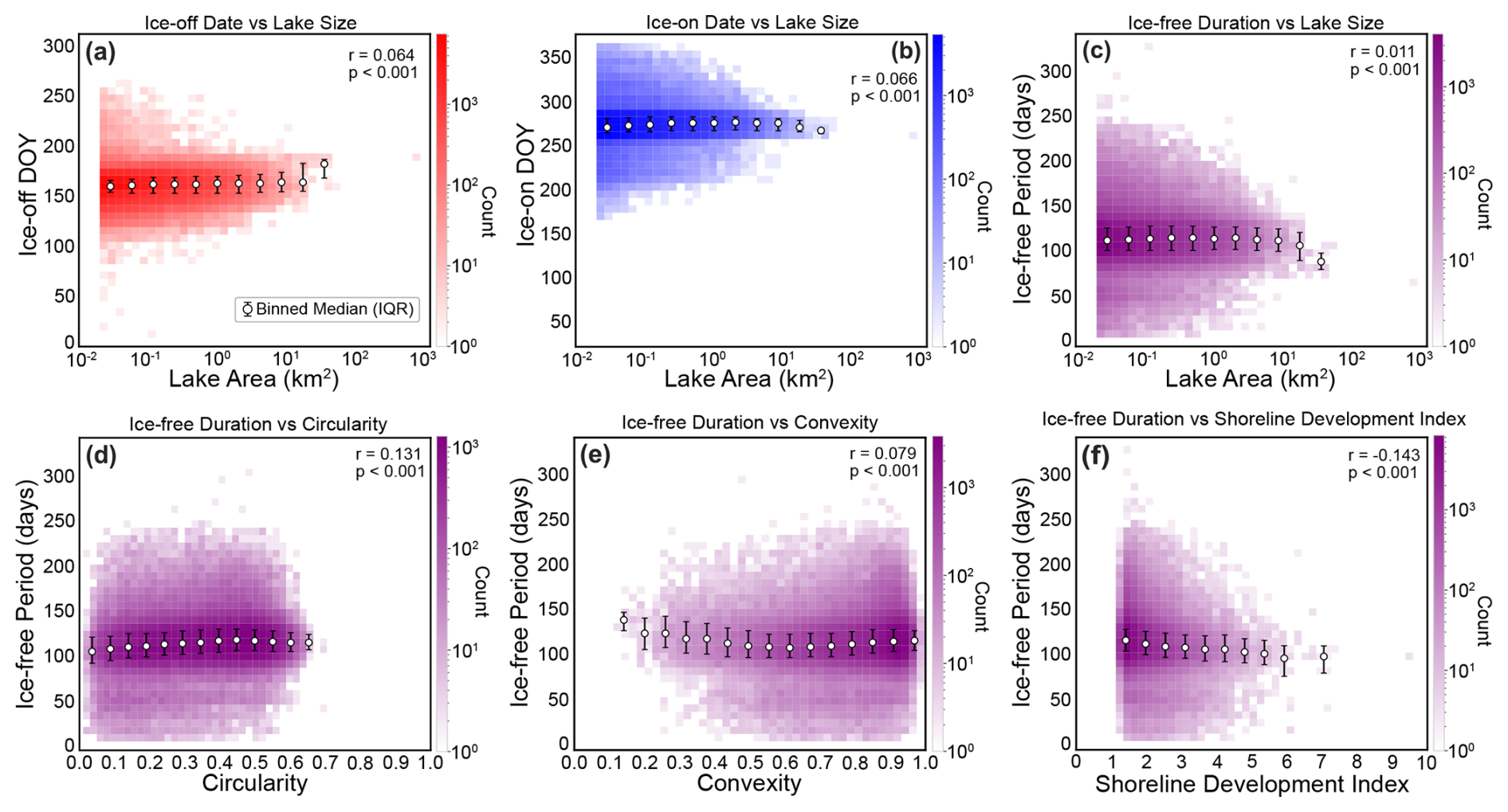
Figure 7 (A) Ice-off dates vs lake area (km²) for all lake-years. (B) Ice-on dates vs lake area for all lake-years. (C) Ice-free duration vs lake area for all lake-years. (D) Ice-free period (days) vs lake circularity for all lake-years. (E) Ice-free period vs lake convexity for all lake-years. (F) Ice-free period vs lake SDI for all lake-years. Ice phenology data here is determined by the SAR RF model. White circles denote the binned median metric and horizontal bars show the interquartile range (25th–75th percentile); bins with fewer than 30 observations are omitted.

3.3 Morphometric relationships

Morphometric variables showed negligible correlations with mean spring temperature ($\left|r\right|$ ≤ 0.11 for circularity, convexity, SDI, and log-transformed area), confirming that morphometry is not confounded with spatial climate gradients. To assess the strength of morphometric controls on ice phenology, we modelled ice-off date, ice-on date, and ice-free duration as functions of mean spring temperature (April–June) and morphometric parameters using ordinary least squares regression. Lake area shows a statistically significant, but negligible correlation with ice-off and ice-on dates and ice-free duration (Fig. 7a–c), indicating that although the relationship is detectable given the large sample size, it explains minimal variation in phenology. Lake circularity, convexity, and SDI exhibit very weak but statistically significant correlations with ice-free duration. Overall, morphometric correlation (area, circularity, convexity, and SDI) with ice phenology (ice-off date, ice-on date, and ice-free duration) is weak (< ± 0.17) (Fig. 8). Morphometry coefficients attenuated by approximately 20 %–25 % under spatial correction but remained highly significant (p < 0.001), confirming that morphometric effects on ice phenology are robust to spatial confounding. Multiple regression with temperature as a covariate showed that morphometric parameters explained an additional 1.5 %–2 % of variance in ice phenology beyond temperature alone. OLS residuals showed significant spatial autocorrelation, so SEMs were used; all morphometric predictors remained significant after this correction, with shoreline development index (SDI) and convexity showing the largest effects.

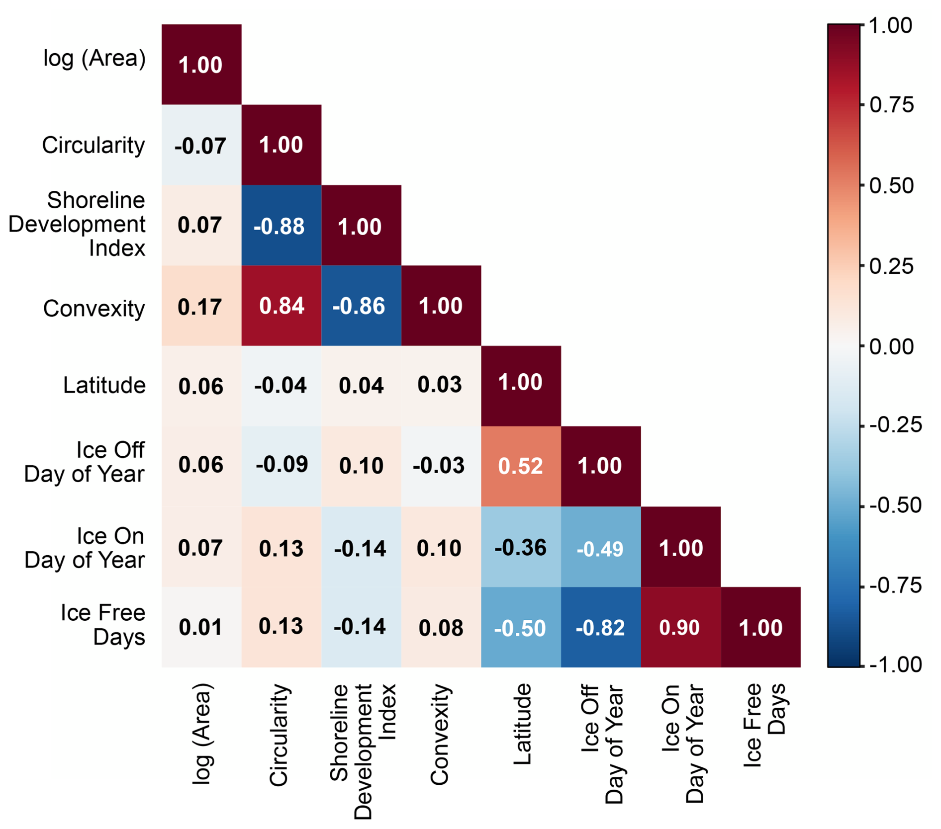
Figure 8 Correlation matrix between lake morphometric variables (log transformed area, circularity, SDI, convexity), latitude (centroid latitude), and SAR RF model-detected ice phenology (ice-off dates, ice-on dates, ice-free days).

Effect sizes using the SEM coefficients were modest relative to temperature and interannual variability. Lakes with more complex shorelines (higher SDI) experienced shorter ice-free seasons (−4.3 d across the interquartile range), as did lakes with higher convexity (−3.5 d). We note that the signs for correlation between morphometric variables and phenology retrievals all stayed the same apart from convexity and ice-free period, where the correlation coefficient is positive (Fig. 7e) prior to using the SEM and negative after accounting for spatial autocorrelation. Lake area and circularity showed smaller effects (+2.7 and +2.4 d, respectively) (Fig. 9). Using the entire data distribution, increasing shoreline complexity and decreasing lake convexity shortens the ice-free period; while increasing lake area and circularity lengthens the ice-free period (Fig. 7).

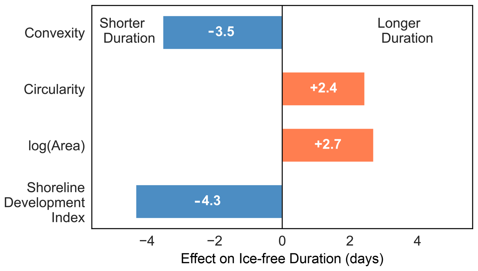
Figure 9 Spatially corrected effect of morphometric variables on SAR RF model-detected ice-free duration, calculated across the interquartile range.

Overall, morphometry plays a subordinate role to temperature in determining ice phenology at the regional scale, with temperature explaining 13 %–19 % of variance compared to 1.5 %–2 % for morphometric parameters. The relatively modest variance explained by temperature reflects the spatial autocorrelation structure in the data: much of the temperature signal is captured by latitude, which is implicitly included through the spatial error model. The spatial error parameter confirms that regional factors beyond point-level temperature such as coastal proximity, local topography, and regional weather patterns contribute substantially to ice timing variability.

4 Discussion

4.1 Model Performance

While previous studies achieved high accuracy (95.8 %) using sophisticated segmentation algorithms and extensive texture features on individual lakes (Hoekstra et al., 2020), such approaches are computationally prohibitive for analysis of tens of thousands of water bodies. Our simplified RF framework using six backscatter features achieves 94 % accuracy while enabling consistent classification of ∼ 30 000 lakes across multiple years, including during polar night and cloudy conditions when optical data are unavailable, demonstrating the feasibility of regional-scale ice phenology monitoring from satellite observations. Previous single-sensor SAR studies typically achieved accuracies on the order of ∼ 80 %–85 % (Surdu et al., 2014). The use of Sentinel-2 optical data to generate training labels for the RF classifier, combined with temperature-based quality control, enabled reliable classification even during the challenging transition seasons. The RF model feature importance (Fig. 2B) further shows that using additional contextual information, such as land buffers surrounding the lakes, increased overall RF model accuracy compared to solely relying on lake pixels for ice-state determination (Tom et al., 2020).

The separability of the probability density functions for lakes without ice phenology compared the total population for SDI and convexity, but not area (Fig. S12), is likely reflective of complex shorelines negatively impacting our ice phenology detection. For example, our algorithm relies on interior buffers that may not perform as well when shorelines are increasingly complex. However, convexity and SDI are likely not the sole reason nor explanation for the phenology not being detected for these lakes, where there are other plausible mechanisms that could explain our algorithm failing for these lakes. The mean ice-free period of 114 d is consistent with limited in situ observations available for the region. Arp et al. (2015) reported ice-free periods of 80–110 d for instrumented lakes on the Arctic Coastal Plain during 2004–2013. Our results extend these findings across the full thermokarst lake population of roughly 30 000 lakes. We do note that there are a small number of statistical outlier lakes (outside ± 2σ) that exhibit phenological events that are physically improbable compared to climate data. For the ice-off metrics, we find that there are 6325 lake-date outliers (4.17 % of total lake-dates). Likewise for ice-on, there are 8641 lake-date outliers (5.27 % of total lake-dates). Here, we note that these outliers comprise approximately 5 % of data and are not representative of the total aggregate population of lake-dates.

The bias in offsets we observe in the ice-off and ice-on dates between the RF model and the ADD estimates are likely due to inherent assumptions made in the RF and ADD models, as well as spatial scale differences in data resolutions (∼ 10 m px⁻¹ for Sentinel-1 vs ∼ 30 km px⁻¹ for ERA5). Additionally, the loss of Sentinel-1B on 23 December 2021 reduced the density of repeat passes and coarsened the granularity of the ice-on/off day-of-year estimates following its failure. However, the RF and ADD models have fair agreeance, but they also exhibit inter-model biases that manifest differently during thaw and freeze. We do not necessarily interpret the offsets between the RF and ADD models as errors, but rather as the expected lag between the onset of freezing or thawing and the lake reaching a fully ice-covered or ice-free state and inherent differences between the accuracy of both models.

The accuracy of the RF model implicitly depends upon the assumed polarimetric scattering model, wherein changes in radar backscatter within and between polarization channels are assumed to be driven by the systematic difference in polarized backscatter between ice and liquid water (Jeffries et al., 1994; Beaven, 1995). In reality, dielectric permittivity changes due to partial surface melting, the presence of snow, changes in snow water equivalent, and ice metamorphism can all introduce changes to SAR backscatter that can complicate the interpretation of a simple water phase transition (Paul et al., 2015; Marin et al., 2020; Lund et al., 2022; Veijola et al., 2024). These confounding effects can be particularly apparent during the shoulder seasons making satellite observation of ice phenology difficult (Posch et al., 2024). Additionally, it is possible that the Sentinel-1 descending track (∼ 61 % of scenes) images, which are acquired between 07:00–09:00 AM AKST, may also introduce variability in predicted ice phenology with the RF model due to diurnal freeze/thaw processes during the shoulder seasons, as compared to the ascending track images acquired between 06:00–08:00 PM AKST (Fig. S8 in the Supplement).

Likewise, the use of ADD to model thermal diffusion through the ice cover implicitly assumes a purely one-dimensional diffusive heat transfer at the air-water surface interface, neglecting lateral heat transfer or wind-driven thermal advection. Additionally, the ADD model does not account for thermal mixing that occurs before ice formation begins. Larger and deeper lakes take longer to mix, which delays ice formation. We expect that the ADD model would likely estimate earlier ice-on dates than when ice formation may actually begin as a result. We further do not consider the effect of snowpack cover, which serves to delay ice-off timing, due to the lack of sufficiently accurate, high spatial resolution snow depth and snow water equivalent products. The 40 cm mean snowpack on the Arctic Coastal Plain reported in Stuefer et al. (2025) is significant enough to insulate the soil and delay ice-off timing.

Consequently, the RF model may be capturing this thermal insulation and relative delay in ice-off timing compared to the ADD model, which is consistent with the observed lag in RF model timing compared to the ADD model for 60 % of lake-year combinations. Our deliberate choice of a relatively simple empirical model might explain some of the observed offset between RF and ADD model ice-on and ice-off calls, particularly during ice thaw when the presence of snowpack can considerably impact the timing of ice-off (Pouw et al., 2023). This epistemic uncertainty propagates into both models' abilities to predict exact dates for ice phenology.

To minimize the potential for an early ice-off bias, our analysis relies on observations from the lake interior rather than the shoreline, where ice loss is expected to occur first because adjacent land surfaces warm more rapidly than the frozen lake. Although ice drifting toward the shore is possible, the interior edge buffer used in this study is only 10 m wide, corresponding to a single Sentinel-1/2 pixel. Given this spatial limitation, we cannot reliably quantify uncertainty or bias associated with potential ice drift within this single-pixel boundary zone. Nonetheless, any remaining risk of an early ice-off bias is further reduced by the temperature-based labelling criterion described in the methodology, which provides an additional constraint on ice-off classification.

The observed offset between the RF and ADD model phenology dates is likely also due to differences between the onset of freezing or thawing and when a lake becomes fully ice free or ice covered. The fact that 60 % of ice-off dates are predicted later by the RF model than by the ADD model may reflect the effects of thermal inertia during spring, where higher air temperatures and ADDT suggest faster ice thinning than is captured by the RF model analyzing lake backscatter. Despite the simple radar scattering and thermodynamic models employed here, each model exhibits decent predictive power for ice phenology and timing, and the inter-model biases are physically consistent.

4.2 Latitudinal and morphometric effects on ice phenology

The primary control on thermokarst lake ice phenology on the Alaska North Slope is latitude, which implicitly includes temperature. Latitude also incorporates other factors such as coastal proximity, elevation, topography, and local weather patterns. As a result, these likely also contribute to ice timing variability in addition to temperature. Even after excluding the high residual lakes primarily associated with the Brooks Range foothills, latitude continues to inform the regression predictor variables (mean spring temperature and morphometric properties). The weak but non-zero latitudinal correlation with residuals (ρ = −0.24) suggests there are still processes that covary with latitude but are not represented in the regression, such as elevation, which may explain the remaining correlation. The strong latitudinal gradient in ice-free duration (23 d per degree northward for lakes with residuals within the 5th–95th percentile of the distribution; Fig. 5) is consistent with the heightened climate sensitivity of lakes near the northern limits of the seasonal ice zone. This sensitivity implies that continued Arctic warming could produce disproportionately large changes in ice phenology for these northernmost lakes, with consequently disproportionate effects on future green-house gas emissions (Walter Anthony et al., 2018).

Our statistical analysis suggests that the offset between the RF and ADD model ice-on and ice-off dates is due in part to latitudinal effects. This is particularly so for lakes for which the RF-ADD model offset is greater than 2 revisit gaps (> 12 d). Lakes at lower latitudes are more likely to have ice-off detected by the RF model earlier than the ADD estimates and ice-on detected later relative to the ADD estimates. Lakes at higher latitudes have ice-off detected by the RF model later than the ADD estimates and ice-on earlier relative to the ADD estimates. This indicates that the RF model detects a longer ice-free period for lower latitude lakes and a shorter ice-free period for higher latitudes relative to the ADD estimates, suggesting that the ADD model is more conservative in predicting ice-free duration at lower latitudes whereas at higher latitudes, the RF model is more conservative.

The latitudinal gradient in offsets between the models may be explained through ice thickness variation as a function of latitude, the RF model not accounting for ice thickness, topography and microclimate, and differences in the spatial resolution of data. Given that lower latitudes have higher temperatures and are located further inland, they may have thinner ice overall and more complex freezing and thawing dynamics than lakes at higher latitudes. Meanwhile, these higher latitude lakes experience cooler temperatures and are more exposed to the Arctic Ocean thus freezing more rapidly. Furthermore, it is likely that the topographic gradient from the Brooks Range in the south to the low-elevation ACP in the north of our study area has an effect on the thermal budgeting of the lakes, owing to high-relief, radiation shadowing, and aspect differences that affect SAR backscatter through the imaging geometry (e.g. layover and shadowing). Additionally, the higher resolution of the SAR observations (∼ 10 m px⁻¹) compared to the ERA5 temperature data (∼ 30 km px⁻¹) may cause the RF model to capture thawing and freezing more precisely than the lower resolution ADD estimates of ice thickness by accounting for other thermal effects around lakes and the local microclimate and topography that are beyond the resolution capabilities of the ERA5 data.

The morphometric relationships we identified provide insight into the physical controls on ice phenology beyond geographic location. Morphology regulates heat transfer from a lake's surroundings to the lake itself (Basu et al., 2024; Brown and Duguay, 2010) ultimately modulating the coupled effects of air temperature and latitude for an individual lake.

Shoreline development index (SDI) and convexity showed the largest effects after spatial correction (∼ 3 d across typical ranges), while lake area and circularity showed smaller but significant effects (∼ 1–2 d) (Fig. 9). Higher SDI, indicating a more complex shoreline, generally suggests shorter ice-free periods, with the onset of freezing occurring earlier in the year and onset of thaw beginning later. Similarly, lower convexity, associated with higher boundary concavity or irregularity (Bozeman and Pilling, 2013), shortens the ice-free period due to ice-on occurring at an earlier date. However, this trend with lower convexity and shorter ice-free periods holds true for the full distribution of lakes in the dataset not accounting for spatial autocorrelation. Conversely, higher circularity lakes tend to remain ice-free longer because they freeze later and thaw earlier in the year.

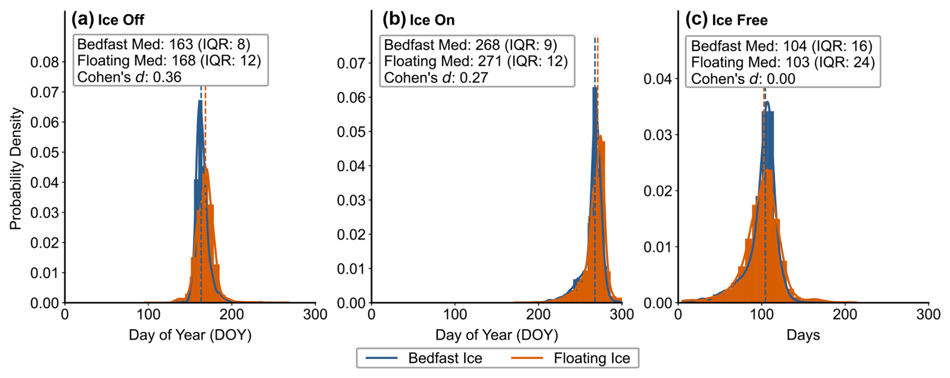
Figure 10 Bedfast and floating ice regime data (Engram 2018; Bergstedt and Jones 2025) histograms and kernel density estimations for (a) ice off, (b) ice on, and (c) total ice-free days across 6797 spatially overlapping lakes with our SAR RF-detected ice phenology events.

These patterns may reflect thermal sheltering in inlets and reduced fetch, which promotes ice growth earlier in the year (Basu et al., 2024). Smaller fetch results in reduced wind speeds, which facilitates the growth of ice crystals, while higher wind speeds can break up the initially forming ice layer. (Brown and Duguay, 2010). Ice growth typically begins along sheltered parts of the lakes and along the shore (Ashton, 1986), due in part to the wind-effect but also because of the shallower depths, which are more sensitive to temperature changes (Kirillin, et al., 2012). Irregular lakes have more shoreline per area, helping to initiate ice growth earlier than more circular or compact lakes. Lower convexity may also be related to overall shallower depths (Zhan et al., 2023), suggesting that deeper lakes have longer ice-free periods than shallower lakes. This likely corresponds to the patterns we identify with lake area, where ice free period increases with lake area. Lake depths tend to scale with area (Cael and Seekell, 2022); thus, these larger and deeper lakes remain ice-free longer because they begin freezing later in the year likely due to a combination of longer periods of thermal mixing within the water column and their greater thermal inertia. Indeed, lake depth has been found to be a significant control on the timing of ice-off conditions for thermokarst lakes in this region (Arp et al., 2015).

Lake depth also serves as a control on which lakes have bedfast or floating ice, which may also influence ice-out timing (Grunblatt and Atwood, 2014; Sellmann et al., 1975). We combined SAR-based lake classifications of bedfast and floating ice regimes (Engram 2018; Bergstedt and Jones 2025) with our SAR RF-detected ice phenology across 6797 lakes overlapping between the combined datasets. We observe that the difference between bedfast and floating ice regime has little effect on ice phenology over this large geographic extent encompassing seven thousand lakes as shown by the relatively small values of Cohen's d separability (Fig. 10). However, we do observe that bedfast ice lakes in the aggregate thaw prior to floating ice lakes in the aggregate; we see a modest five-day difference in median values between bedfast and floating ice for ice off compared to the larger 16 d difference found in Arp et al. (2015).

While a highly correlated scaling between lake depth, area and ice-free uration remains outstanding – potentially due to the limited range of thermokarst lake depths, and the importance of the underlying substrate (Hinkel et al., 2012) – some studies have shown moderate correlations between lake depth and area (Arp et al., 2011), with modelling suggesting physical mechanisms by which lake deepening and enlargement can occur (Ohara et al., 2022). We therefore suggest a very general correspondence between these morphometric properties, which allows for the observed variability we identify.

Overall, morphometry explained only 1.5 %–2 % of variance beyond temperature, indicating that climate remains the dominant control on regional ice phenology. Nonetheless, morphology plays a significant role in regulating the climatic impact for thermokarst lakes on the Alaska North Slope.

4.3 Implications for GHG emissions and Arctic change

Based on our results, Arctic thermokarst lakes are likely to experience pronounced effects on ice phenology due to global climate change. The strong latitudinal-temperature dependence suggests that increased warming will likely increase the ice free-period, which will further contribute to greenhouse gas emissions (Guo et al., 2020; Zhuang et al., 2023). Because larger lakes have longer ice-free durations, their potential contribution to GHG emissions may increase. However, these effects may be dwarfed by the sheer number of smaller lakes, which likely have a higher potential contribution. Furthermore, if larger lakes are indeed deeper, than they may also be less efficient emitters of methane due to increased oxidation that occurs in deeper water columns. Recent work (Levenson et al., 2025) found that thermokarst lakes in previously unglaciated landscapes underlain with continuous permafrost, including our study area, are projected to decrease in overall total area under projected climate scenarios. This reduction in total area may have direct effects on average lake depth and consequently emission potential, as shallower lakes and ponds exhibit higher methane emissions than deeper lakes (Manasypov et al., 2023).

Other climatic processes that depend upon the timing of ice formation and breakup may also be affected by a changing global climate. Evaporative fluxes from ice-free lakes increase substantially following ice-out, enhancing the exchange of moisture and heat between lakes and the atmosphere. As demonstrated by Arp et al. (2015), variations in lake depth, ice thickness, and ice-out timing can lead to divergent hydrologic responses among lakes in this region, further highlighting the potential importance of lake morphology in modulating lake ice phenology and its impact of climate processes.

The phenology baseline established here provides a foundation for detecting future changes in thermokarst lake ice regimes that can be incorporated with other Arctic remote sensing studies of methane emissions from thermokarst lakes (Elder et al., 2020; Engram and Walter Anthony, 2024; Kyzivat and Smith, 2023). Future monitoring efforts can be leveraged in conjunction with these results to assess whether ice-free periods increase as predicted by climate models. Lastly, upcoming higher-resolution spaceborne methane measurements (e.g., MethaneSAT, Carbon Mapper, GHGSat; McLinden et al., 2024) could be leveraged in conjunction with this ice phenology and timing observational method to directly observe the ice-phenology-emission relationship from the individual lake-scale to the regional-scale and determine the relative importance of numerous small lakes vs. fewer larger lakes in consideration of GHG emission budgeting.

5 Conclusion

This study presents the first comprehensive analysis of ice phenology across the Alaska North Slope thermokarst lake population. Using a RF classifier trained using labels derived from Sentinel-2 optical imagery and ERA5 temperature data and applied to Sentinel-1 SAR imagery, we achieved 94 % accuracy for ice state classification and retrieved phenology for 30 774 lakes over five years (2019–2023).

The mean ice-free period is 114 d, with ice-off occurring in mid-June (DOY 159) and ice-on in late September (DOY 273). Latitude exerts dominant control on ice timing, with ice-free duration decreasing by 23 d per degree northward. Morphometric predictors showed modest but significant effects after spatial correction, with shoreline development index and convexity each contributing ∼ 3 d variation across typical lake ranges.

These results provide essential baseline data for monitoring how thermokarst lake dynamics respond to continued Arctic warming, with implications for regional carbon cycling and climate feedbacks. The lake-specific ice phenology dates also provide critical timing constraints for methane emission models and for planning targeted high-resolution observation campaigns.