The implementation and effectiveness of Calving Algorithms in numerical ice models (CalvingMIP)

Ice calving plays a significant role in ice sheet mass loss. Predictions of future ice sheet mass balance require accurate representations of the calving process in numerical ice models to determine rates of future global mean sea level rise. Whilst calving has recently begun to be implemented in numerical models there has not yet been a systematic investigation into how this implementation compares between different ice flow models. The Calving Model Intercomparison Project (CalvingMIP) has been established to address this question by providing a framework of experiments to investigate the accuracy of simulated calving rates and how simulated properties at the calving front evolve over time. Our initial focus has been on how calving is implemented in models, therefore focusing on calving algorithms, rather than on how much ice should be calved at a particular time via a calving law. Our results, from thirteen different numerical modelling groups, show that the majority of calving algorithms implemented are able to accurately implement a given calving rate with an ice front that evolves smoothly throughout the calving process, albeit with slightly more variation of results in a more complex domain. These results show that we can have confidence in the models capacity to accurately implement calving laws in the future.

1 Introduction

Ice sheets lose mass via two primary processes, melting and calving. For the Greenland and Antarctic ice sheets, calving represents approximately two thirds and one half of ice loss, respectively (Mouginot et al., 2019; Greene et al., 2022). Despite its importance and potential for destabilisation of ice flow via its impact on ice shelf buttressing and extent, calving remains poorly represented in current state-of-the-art ice sheet models. Whilst parameterised ice shelf melting has been a widely used feature in ice shelf models (e.g. Beckmann and Goosse, 2003; Lazeroms et al., 2018; Reese et al., 2018) as well as direct ice-ocean coupling to generate melt rates (e.g. De Rydt and Gudmundsson, 2016; Jordan et al., 2018; Favier et al., 2019) for decades, ice-shelf calving is only now becoming a feature widely used in numerical ice models. Many large scale models often consider the calving rate to be equal to the ice velocity at the calving front, which means that the calving front remains fixed over time (Seroussi et al., 2020). One main reason for this simplification is that implementing ice-shelf calving in numerical models is a non-trivial problem due to processes operating at widely varying spatial and temporal scales, with a step change moving boundary between ice and ocean combined with observed individual calving events occurring in a semi-stochastic fashion. Correctly implementing them in large scale models requires a significant amount of time and additional computational resources.

Efforts are further hampered for Antarctic ice shelves by the lack of long term observational data sets to calibrate and validate numerical models of calving, with calving cycles tending to a period of slow advance over potential decades followed by a large calving event inducing rapid retreat (e.g. Cook Glacier; Miles et al., 2018). The satellite observational record operates on a similar time scale, giving a distinct lack of observations spanning numerous calving cycles at the same location, though more detailed time series of recent years are now available (Baumhoer et al., 2023). Despite these obstacles, developing an accurate framework for representing calving in numerical ice models is of critical importance for making accurate and reliable predictions of the ice sheets' contributions to sea level rise.

In a stand-alone ice sheet model, the sensitivity to changing rates of calving front retreat can be comparable to that of changing ocean-induced basal melt (Barnes et al., 2026), but to date far less progress has been made towards achieving representation of realistic calving in models. In the ISMIP6 experiments (Seroussi et al., 2020), 6 out of 17 models maintained a fixed calving front position, whilst the rest implemented some form of calving law. The most commonly used calving laws are von Mises calving (Morlighem et al., 2016), eigencalving (Levermann et al., 2012), or calving based on crevasse depth (e.g. Benn et al., 2007; Nick et al., 2010) or cliff heights (e.g. Pollard et al., 2015; Crawford et al., 2021). Some existing calving laws have been evaluated across glaciers in Greenland (Choi et al., 2018) and Antarctica (Wilner et al., 2023) in a single model and, although no particular law was seen to consistently reproduce observed calving fronts, eigencalving and von Mises were found to be the best performing calving laws (Wilner et al., 2023). These approaches remain marginal, and have never been clearly evaluated in a multi-model environment with an investigation of their impact on sea level rise contribution. As calving is a stochastic process, there remains debate about how best to evaluate model performance when compared to the observational record.

The Calving Model Intercomparison Project (CalvingMIP) is a community driven effort to address these issues. It is the first attempt to assess the current state of calving in numerical ice sheet models and set a baseline to accurately simulate this critical process. Whilst the initial driving force behind CalvingMIP came from the European Union funded Horizon 2020 project PROTECT, it has grown to incorporate members from across the wider cryospheric modelling community, with thirteen participating modelling frameworks. Further information on CalvingMIP can be found on the project's web page (https://github.com/JRowanJordan/CalvingMIP/wiki, last access: 1 November 2026).

Throughout this work we find it helpful to define some key terms regarding the numerical implementation of calving within ice models. We make a clear distinction between a calving law and a calving algorithm. The term calving law is well established in the field and refers to the amount of ice that should be calved based on the physical properties of the ice, with the calving law producing a calving rate or prescribing a calving front position. This could be as simple as removing all ice below a certain critical thickness threshold at daily intervals or a more complex process based on stress and strain rates within the ice itself and how they interact with a separate damage model that evolves over centuries. We define a calving algorithm to be the process by which a numerical model implements a calving law and removes the required amount of ice. The term calving is often used to cover a range of temporal and spatial scales, from an individual calving event on a single tidewater glacier in Greenland to the long term evolution of the calving front position over several centuries for the entire Antarctic Ice Sheet. We hereby define discontinuous calving to be primarily focussed on high resolution simulations of individual calving events whilst continuous calving is primarily focussed on large scale simulations that lack the resolution in both space and time to simulate individual calving events. Continuous calving may be thought of as the long term average of a series of discontinuous calving events.

The first phase of CalvingMIP experiments, which we present the results of here, are focused on continuous calving over hundreds of years on large scale domains. We do not see continuous calving as the optimal way of representing calving, but given current model limitations and understanding of the physical processes behind calving it is likely to be the dominant method used in large scale predictions of future ice sheet mass balance for the foreseeable future. An increased awareness of its capabilities and limitations are desirable, both in its own right and as a stepping stone to more sophisticated calving algorithms. As such, we focus here on the technical challenge of implementing a continuously evolving calving front.

The results of CalvingMIP experiments are not intended to show a “best” or “worst” participating model but are instead intended to accurately showcase the current state of the science in regards to implementing calving in numerical models. To this end, when comparing results between participating models, we have four key principles that we believe models should strive to adhere to if they seek to accurately apply a calving rate derived from a calving law to their particular calving algorithm. These are;

• Models should be able to accurately apply a given rate of ice-shelf calving. As a fundamental principle, we believe that confidence is needed in a models ability to calve the correct amount of ice and remove it from the model domain. Until we have this confidence, then there is limited benefit in improving existing calving laws. Additionally, front position should be accurately tracked across the subgrid scale, as a calving front's rate of retreat in reality is unlikely to neatly line up on model grid boundaries.

• Ice properties at the calving front should evolve smoothly in time. Calving rates generated by a calving law simulating continuous calving are likely to be highly dependent on ice properties at or near the calving front. If these change rapidly in response to shifting the calving front position, then there is the possibility of oscillating calving rates driven by model numerics rather than physical processes. Note that in simulations of discontinuous calving, we would expect there to be more abrupt changes in calving front properties following an individual large calving event.

• The effect of calving should be independent of model orientation. All else being equal, the effect of calving on the front position should be independent of orientation in respect to the model grid or mesh.

• The impact of calving upon overall ice extent, grounding line position and the ratio between floating and grounded ice is of key importance. Whilst it is impossible to define a correct answer as to how models should behave in this regard a priori (unlike our other principles) this is of crucial interest when determining future ice sheet mass balance and contribution to sea level rise, and so is an important point of comparison between model outputs.

Here we show results for 13 different numerical ice-model configurations performing the first phase of CalvingMIP experiments. Models are compared on their ability to implement a calving algorithm applying a given calving rate in both a highly simplified circular domain (with an exact, analytical solution for calving front position in time) as well as an idealised, synthetic ice sheet with more complex bathymetry. We show how calving front position as well as ice properties at the front evolve over time as well as the impact of calving on model symmetry and ratio of floating to grounded ice. This is the first comprehensive analysis of a large number of numerical ice models that have implemented calving in the same prescribed experiments. It is our hope that as well as serving as a useful reference in and of itself, this work will be a vital first step towards future efforts to numerically simulate calving.

2 Experimental Design

Our experiments encompass two domains. The first has minimal variations in bedrock bathymetry and is intended to be a pure test of the calving process, with variations from other factors such as bedrock bathymetry minimised. The second domain introduces some variation in the bedrock bathymetry which will promote the formation of different types of ice shelf within the same domain and is intended to test models' responses in a more complex domain.

Prior to undertaking the experiments, each model is initialised from an ice free state by applying a constant and uniform positive surface mass balance of 0.3 m a⁻¹ over the entire domain. A fixed, unmoving, circular calving front with a radius of 750 km from the centre of the domain is imposed, and the model is then required to be run until a steady state is achieved. Note that, in these particular experiments, we are not interested in the exact means by which this steady state condition is achieved but instead are concerned with all models having a comparable steady state. Participants were free to spin up their ice model without a calving front, subsequently impose a calving front, and then run their model to a steady state if they preferred. The main experiments use this steady state initialisation for each domain as the initial conditions. In the main experiments, the models are allowed to evolve over 1000 years with the rate of retreat of the calving front specified by a given calving rate. For the first 500 years of the experiment the calving front will be made to retreat, before advancing for the second 500 years.

2.1 Circular Domain

The first domain, hereafter referred to as the Circular Domain, has a circular symmetry with a smoothly rising dome of bedrock in the centre of the domain (Fig. 1). The bedrock elevation, B, is defined as a function of radius, r, from the origin, such that;

$$\begin{array}{}\text{(1)}& B=B_c-\left(B_c-B_l\right){\left({\displaystyle \frac{r-r_c}{R-r_c}}\right)}^{\mathrm{2}}\end{array}$$

where R = 800 km, B_c = 900 m, B_l = −2000 m, and r_c = 0 m. The domain's total area is approximately a quarter of the size of the Antarctic Ice Sheet providing a good scale for the intended use of the numerical models and types of calving we are investigating.

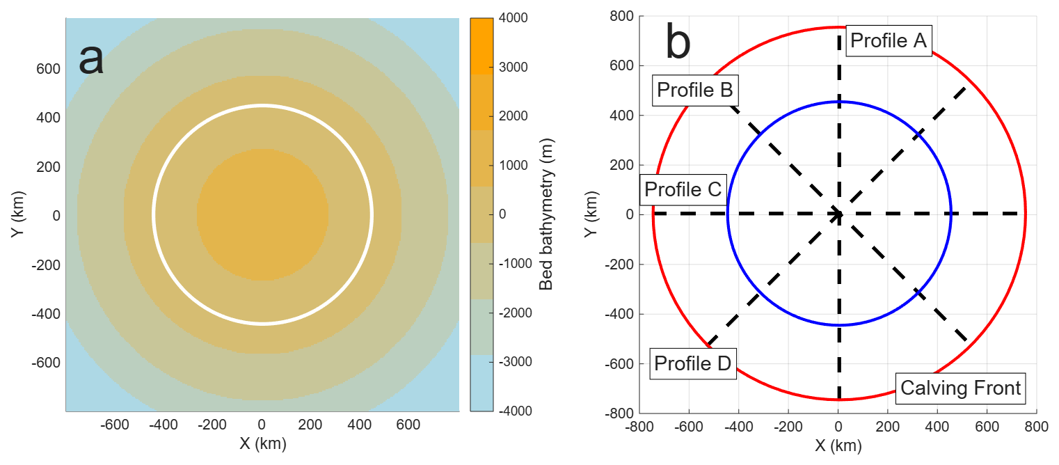
Figure 1 Circular Domain. (a) Bedrock bathymetry (with the sea level contour shown in white) and (b) schematic diagram of results profiles (with initial calving front position shown in red, sea level contour in blue, and line profiles in black) of the Circular domain.

This domain is intended to test a number of aspects of implementing a calving algorithm within a setup where the simulated calving front position can be directly compared to the exact solution. This experiment will test models' capabilities to not only retreat a calving front but also allow it to advance again. The calving rate to be imposed, and hence ice front position, has also been deliberately chosen to vary in time and thus not be a neat multiple of model grid resolution. This will require participating models to utilise a method for tracking the position of the calving front at the sub-grid scale to accurately track its position over time. The rate of advance has also been chosen to be less than the simulated ice velocity at the calving front, as having an imposed calving front advancing more rapidly than the ice velocity at the calving front would be unphysical. By specifying a perfect circle that contracts and expands in time as the calving front boundary we also enable easy testing of model symmetry when utilising discrete grids or meshes. As the ice shelf is a perfect circle with no obstructing bathymetry, and we specify the precise amount of ice front position change at any given time, it is possible to have a “known” solution of ice front position to compare models performance to.

2.2 Thule domain

The second domain for CalvingMIP uses a synthetic ice sheet with a mathematically defined bedrock bathymetry which we refer to as Thule. Thule's bathymetry is designed to promote the formation of a range of ice shelves, both heavily confined and more open, allowing experiments to cover different styles of ice shelf within a single model domain. The bedrock elevation, B, is defined as a function of the polar coordinates, r and θ, as

$$\begin{array}{}\text{(2)}& B=B_a\cos \left({\displaystyle \frac{\mathrm{3}\mathit{\pi }r}{l}}\right)+a\end{array}$$

where

$$\begin{array}{c}{\displaystyle }l=R\left(\mathrm{1}-{\displaystyle \frac{\cos \left(\mathrm{2}\mathit{\theta }\right)}{\mathrm{2}}}\right)\\ {\displaystyle }a=B_c-\left(B_c-B_l\left({\displaystyle \frac{r-r_c}{R-r_c}}\right)\right)\end{array}$$

and R = 800 km, B_c = 900 m, B_l = −2000 m, B_a = 1100 m, and r_c = 0 m.

The model domain is similar in size to the Circular domain, representing an area a quarter that of the Antarctic Ice Sheet. Unlike the circular domain, the Thule domain has at least two possible steady states depending on whether the simulation spins up from zero initial ice thickness or has a large initial ice thickness. For our experiments, the intended steady state is that which is achieved from zero initial ice thickness, with the ice ungrounded from the Benett underwater ridges located under the North and South Tsalal ice shelves (see Fig. 2). Whilst none of the participating models encountered issues with this, if different models attempt to carry out our experiments in future it may be necessary to tune the suggested experimental parameters (bed slipperiness, etc.) to achieve a comparable steady state.

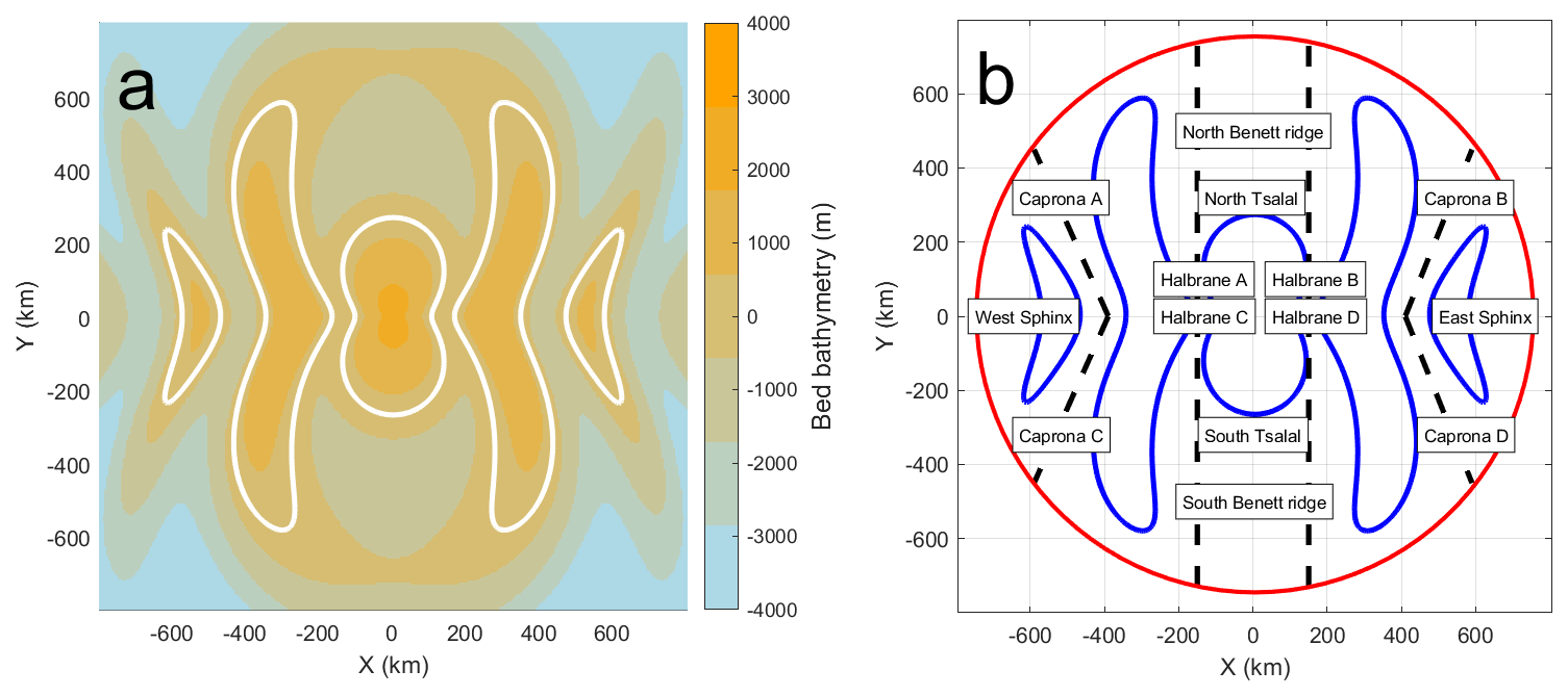
Figure 2 Thule Domain. (a) Bedrock bathymetry (with the sea level contour shown in white) and (b) schematic diagram of results profiles (with initial calving front position shown in red, sea level contour in blue, and line profiles in black) of the Thule domain. Names of the various geographical features of Thule are also shown.

The Thule domain experiment is intended to investigate the effect of an imposed rate of calving front retreat and advance with more complex, but still idealised, bedrock geometry. The extent of calving front retreat is such that we would expect to see a corresponding change in grounding line position due to changes in ice shelf buttressing. Knowing if different models experience a difference in the rate or extent of grounding line retreat will be of importance for putting future CalvingMIP experiments in their proper context. This experiment is also intended to test the symmetry of model results, with profiles of results over geometrically identical bathymetry. We specifically do not allow grounded ice to calve in this domain. This will result in a more complex velocity field, with the choice of where exactly the velocity is considered to be “at the calving front” likely to have an impact on the exact pattern of calving front retreat.

2.3 Ice-shelf calving

Our intent for this first phase of CalvingMIP is to compare different models' calving algorithms, with a focus on continuous calving. To that end, we are not focused on discrete calving events but are instead interested in the longer term trends that arise from a series of individual calving events. In the absence of any calving, the position of the calving front would be expected to evolve in time in line with the ice velocity at the calving front. If this long term average calving rate is expressed in terms of meters of ice calved per unit time (in other words, as a velocity), then we would expect the rate of change of the calving front position in time to be given by:

$$\begin{array}{}\text{(3)}& {\dot{W}}_{\mathrm{v}}=I_{\mathrm{v}}-C_{\mathrm{r}}\end{array}$$

where ${\dot{W}}_{\mathrm{v}}$ is the rate of change of the front position in time, I_v the ice velocity at the calving front and C_r the calving rate. Note that C_r is always positive, with a minimum value of 0. A few interesting points arise from Eq. (3). Firstly, if I_v is equal to C_r then W_v will be zero; the ice front is not moving and is in steady state. Secondly, if I_v is less than C_r then W_v is negative and the calving front is retreating. Thirdly, if I_v is greater than C_r then W_v is positive and the calving front is advancing. Note that the maximum rate of front advance occurs when the calving rate is equal to zero and is the same as the ice velocity at the calving front. Our experiments will encompass both a phase where the calving front retreats and also when it advances to cover the full range of calving processes. Finally, we have been deliberately ambiguous as to the exact direction the calving rate is to be applied. Two valid interpretations of this would be to either apply a calving rate that is perpendicular to the ice front position or to apply a calving rate that is parallel to the ice velocity at the calving front. We leave it up to individual models to define precisely how they have applied the specified calving rate. Note that in the circular domain this has minimal impact, as the ice velocity at the calving front is always perpendicular to the ice geometry at the calving front. In the Thule domain, however, this is not the case and ice velocity is not always perpendicular to the ice front geometry.

In regards to ice-shelf calving used in CalvingMIP, the only requirement we impose upon participants is that they are able to implement calving in the above fashion, representing long term trends in calving front position in terms of meters per year advanced or retreated. We deliberately do not impose further restrictions and limitations to allow as wide a participation as possible.

2.4 Imposition of calving front position

To achieve a particular rate of position change in the calving front we impose a calving rate such that the difference between this imposed calving rate and the ice velocity at the calving front is equal to the desired rate of change in calving front position. This means that if two participating models have different ice velocities at the calving front they will need to impose a different calving rate from each other to achieve the same rate of position change. For both experiments we seek to simulate a calving front rate of change of position varying in a sinusoidal fashion for the 1000 years of the simulation. For the first 500 years the calving front position retreats before advancing in the second 500 years of the simulation.

In the case of the Circular Domain the retreat rate reaches a maximum of 300 m a⁻¹ after 250 years, is zero at 500 years and then reaches a maximum advance rate of 300 m a⁻¹ after 750 years. The rate of calving front position change (${\dot{W}}_{\mathrm{v}}$) at a given year (t) is therefore given by;

$$\begin{array}{}\text{(4)}& {\dot{W}}_{\mathrm{v}}=-\mathrm{300}\times \sin \left({\displaystyle \frac{\mathrm{2}t}{\mathrm{1000}}}\right)\end{array}$$

with ${\dot{W}}_{\mathrm{v}}$ positive for an advancing calving front, negative for a retreating. The calving rate required to achieve this value of W_v can then be calculated using Eq. (3).

Similarly, for the Thule domain the imposed rate of calving position change varies in a sinusoidal fashion for the first 500 years. The retreat rate reaches a maximum of 750 m a⁻¹ after 250 years before reducing to zero at 500 years. The rate of calving front position change (${\dot{W}}_{\mathrm{v}}$) at a given year (t) is given by;

$$\begin{array}{}\text{(5)}& {\dot{W}}_{\mathrm{v}}=-\mathrm{750}\times \sin \left({\displaystyle \frac{\mathrm{2}t}{\mathrm{1000}}}\right)\end{array}$$

The calving front position is not allowed to retreat over the grounded ice, therefore imposing a limit on the calving rate at the grounding line. This condition was imposed to allow for the greatest participation amongst models, even if it does result in some potentially unphysical conditions, with thick sheer ice cliffs right at the grounding line in some locations.

For the second half of the experiment the ice front is allowed to freely advance, with a calving rate of 0 m a⁻¹ imposed. This is intended to sidestep any potential issues that may occur if the ice velocity were to be less than the rate of calving position advance if it followed a sinusoidal rate of advance like the circular domain. We also recommend that the calving front does not advance past its initial position to prevent any issues arising from ice advancing past the initial model domain boundary. Some models have chosen to allow this as they encountered no such problems.

2.5 Physical constants and model parameters

Whilst our intention is to specify as little as possible to allow greater participation, some amount of specificity is unavoidable. To that end, we recommend that all participants use a Weertman style sliding law in their ice model, such that the basal sliding velocity, u_b, is given by:

$$\begin{array}{}\text{(6)}& u_{\mathrm{b}}=C{\mathit{\tau }}_{\mathrm{b}}^m\end{array}$$

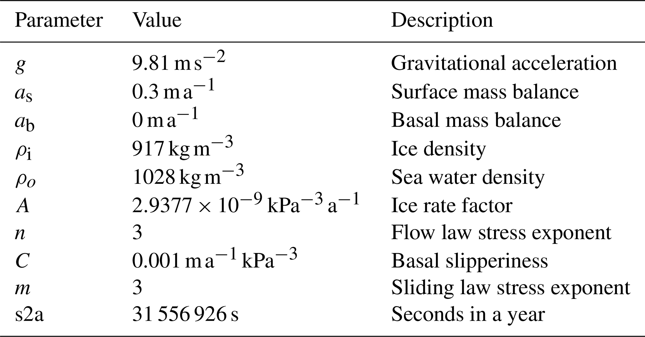
where C is the basal slipperiness and τ_b the basal shear stress with its corresponding exponent, m. We specify that no basal melting be applied at any point of the experiments alongside a uniform and constant, positive surface mass balance. There are no requirements on model resolution or time step beyond the fact that participants should be convinced that their results have converged with both. Models may be two or three dimensional, finite element or finite difference. All results are interpolated onto a regular, 5 km resolution results grid to allow for ease of comparison no matter what there native grid is. A summary of specified parameters can be found in Table 1.

Table 1 Specified parameters for both the circular and Thule domain experiments.

3 Description of participating models

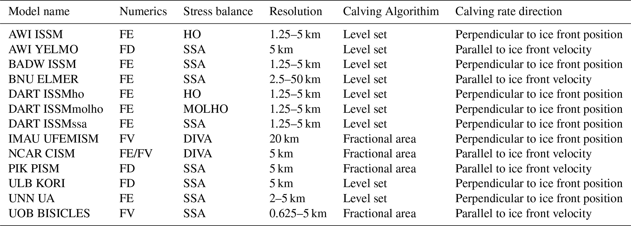
A summary of the participating model groups and contributors is given in Table 2 with an overview of the model properties given in Table 3. More in depth descriptions are given below in individual model sections. Two main approaches have been taken towards calving algorithms, either a level set method or a fractional area method. The level set method utilises a two dimensional field with a specified contour line representing the calving front. The position of this contour line is advected in time based on the ice front rate of change (Eq. 3) with ice removed from cells as calving once the contour moves over them. In the fractional area method a horizontal calving rate is scaled by the ice thickness of a model cell at the calving front to define a negative volume flux (Albrecht et al., 2011). This rate of ice loss can then be tracked by a value representing the fraction of a “full” cell that ice in the model cell at the calving front would fill, removing ice when the fraction falls below a critical value. Both approaches will typically remove ice during the update ice thickness part of a time step, similarly to how ice melting and precipitation are applied. As previously discussed, some models apply their calving rates perpendicular to the ice front position whilst others apply a calving rate parallel to the ice velocity at the calving front. In the circular domain these are the same, but in the Thule domain they will differ.

Table 2 List of participating models, research institutions and contributors.

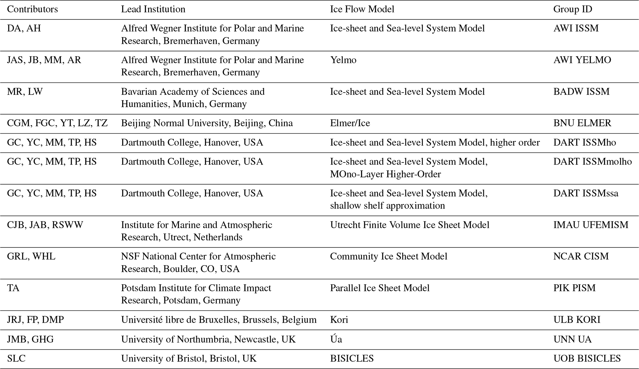
Table 3 Summary of model properties. Numerics are defined as finite element (FE), finite difference (FD) and finite volume (FV). Stress balance is defined as shallow shelf approximation (SSA), higher order (HO), mono layer higher order (MOLHO) or depth integrated viscosity approximation (DIVA).

3.1 BISICLES

BISICLES (Cornford et al., 2013) is a finite-volume adaptive-mesh model. For CalvingMIP, ice velocities are computed according to the shallow-shelf approximation. The computational mesh comprises square cells with resolution varying from 5 km in the interior to 0.625 km around the grounding line and calving front. All quantities are defined at cell centres, and where CalvingMIP analysis requires data located elsewhere, data from the nearest cell centre are provided.

A pseudo-volume-of-fluid (pseudo-VOF) method is used to capture the location of the calving front. VOF methods (Hirt and Nichols, 1981) store a cell-centered volume fraction (in this case an ice area fraction) f in addition to the typical fluid quantities (e.g. ice thickness). A cell is considered ice filled when f = 1, empty when f = 0, and partly ice filled when 0 < f < 1. The area fraction evolves over time according to the non-conservative advection equation

$$\begin{array}{}\text{(7)}& {\displaystyle \frac{\partial f}{\partial t}}+\left(\mathit{u}-\mathit{c}\right)\cdot \mathbf{\nabla }f=\mathrm{0}\end{array}$$

where u is the horizontal ice velocity, c is the calving vector and ∇ is the horizontal gradient operator. The higher-order numerical method (Colella and Woodward, 1984) used to solve the advection equation leads to some front broadening, resulting in a psuedo-VOF treatment rather than a true VOF treatment. For the CalvingMIP submission, c is set antiparallel to u but it can also be set parallel to ∇f.

Models that employ level set methods solve the same equation: the difference is in the assumed meaning of f. The VOF approach works well for BISICLES because it allows the model to define two key quantities. The first is a cell-centered ice loss rate, based on the difference in f between free advance (c=0) and advance/retreat with calving (c≠0). The second is an effective calving front ice thickness $h/f$ for use in calving laws, where h, the mean ice thickness in a cell, is the conserved quantity representing ice thickness.

3.2 CISM

The Community Ice Sheet Model (CISM; Lipscomb et al., 2019) runs on a structured horizontal grid with ice thickness H and other scalars located at cell centers, and ice velocity v at cell corners. For CalvingMIP, CISM solves for velocity based on the Depth-Integrated Viscosity Approximation (DIVA; Goldberg, 2011), and ice is transported using the incremental remapping scheme described by Lipscomb and Hunke (2004). The subgrid grounding-line position is based on a flotation criterion (Leguy et al., 2021).

In CISM's subgrid calving front (CF) parameterization, floating cells adjacent to one or more ice-free ocean cells are identified as CF cells. The effective ice thickness H_eff in a CF cell is computed as the maximum thickness in adjacent floating interior cells, similar to Albrecht et al. (2011). If $H/H_{\text{eff}}$ exceeds a prescribed ratio close to 1.0, the CF cell is labeled as full, and ice in the cell is allowed to advance downstream. Otherwise, the cell is labeled as partly full with area fraction f = $H/H_{\mathrm{eff}}$, and ice cannot advance until the cell is full. The lateral calving rate C_r (positive by definition) is computed as the difference I_v−W_v, where I_v is the ice velocity at the CF, and W−v is the prescribed rate of change of CF position (see Sect. 2.3). The lateral rate C_r is converted to a rate of thickness change $\mathrm{d}H/\mathrm{d}t=-H_{\text{eff}}L{C}_{\mathrm{r}}/A$, where L is the calving front length (e.g. the length of a cell edge) and A is the cell area. The calving front location is not tracked explicitly. Instead, it is estimated by computing f at each cell center and interpolating to find the point along a given axis where f = 0.5.

3.3 Elmer/Ice

Elmer/Ice (Gagliardini et al., 2013) contributed with a vertically integrated model using the SSA approximation to the Stokes equations (MacAyeal et al., 2015). This implies that the grounding-line position is simply a consequence of the floatation criterion. The mesh for both domains was created with Gmsh (Geuzaine and Remacle, 2009) using a quadratic bounding box of 1600 km side-length with a circular region of higher mesh resolution of 2.5 km stretching from 300 to 760 km radius from its centre. This covers the calving-front as well as the grounding-line position in all experiments. Outside this region, the resolution is linearly increased to 20 km towards the bounding box corners and up to 50 km to its centre. The hybrid mesh consists of quadrilaterals in the highly resolved part and triangles outside. Elmer/Ice applies the Finite Element Method, using standard Galerkin formulation with linear functions. In CalvingMIP a level-set method based on the signed distance to the calving front – indicated by the zero-value of the level-set – is used, accompanied by an algorithm that switches elements for both, the solver computing the velocities and the one computing the thickness evolution, to passive at positive and active at negative values of the level-set function. In this application, Elmer/Ice utilized a shared memory parallel computation paradigm (OpenMP threads), resulting in runtimes of a few hours (using a time-step size of 1 year) on a single node of a supercomputer employing 64 cores at a time. Time-steps are taken implicitly and discretized using a backward Euler method. The solution of the linear system is achieved by the Bi-Conjugate Gradient stabilized (BiCGStab, van der Vorst, 1992) method – in the case of SSA preconditioned using an Incomplete LU-factorization (ILU). The non-linear problem is iterated using a Newton method.

3.4 ISSM

Six model configurations based on Ice-sheet and Sea-level System Model (ISSM, Larour et al., 2012) participated in CalvingMIP. The setup of each ISSM submission is summarized in Table 4. Two types of domain geometries were used: circular domains with a radius of 800 km for EXP1 and EXP2 (ISSM Dart), and square domains with a side length of 1600 km for all other experiments. All simulations utilized ISSM's built-in triangle mesh generator (Shewchuk, 1996) to create unstructured, isotropic meshes, with horizontal resolutions ranging from 1.25 to 5 km depending on the specific experiment.

Table 4 Configurations of ISSM submissions.

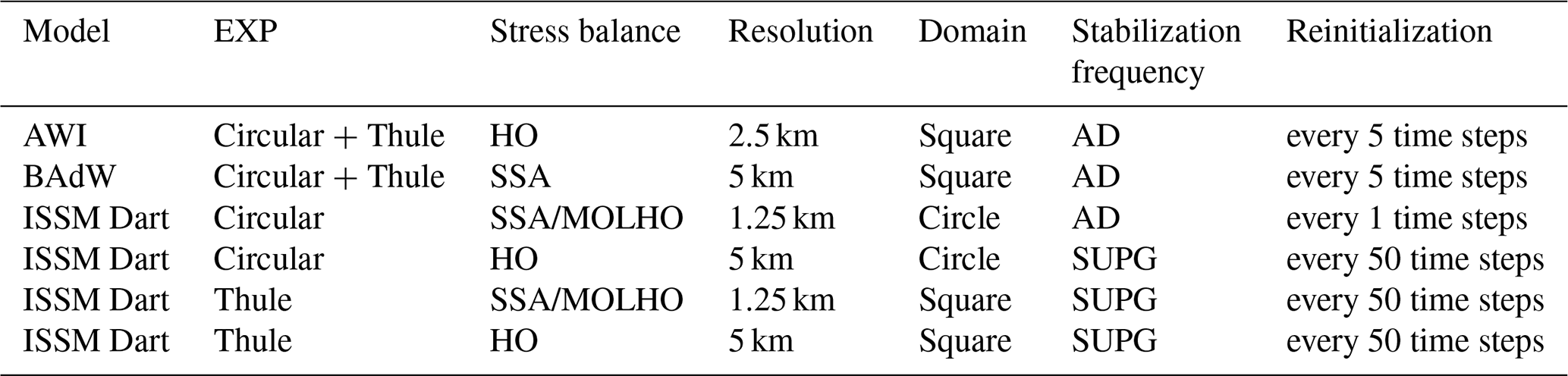
Of the six ISSM configurations, two employ the SSA, two employ MOno-Layer Higher-Order (MOLHO, Dias dos Santos et al., 2022), while the other two use Blatter–Pattyn (HO, Pattyn, 2003) model. SSA and MOLHO simulations are based on 2D meshes with horizontal velocities, whereas HO simulations employ 3D meshes with seven vertical extruded layers in the ISSM Dart configuration and ten layers in the AWI submission. Notably, the horizontal velocities in SSA are depth averaged velocities, whereas in MOLHO, these are the basal and shear velocities.

Ice front migration is implemented in ISSM using a level-set method (Bondzio et al., 2016). All ISSM submissions use numerical stabilization method based on either Artificial Diffusion (AD) or Streamline Upwind Petrov Galerkin (SUPG) method (Cheng et al., 2024). As discussed in Cheng et al. (2024) the level-set function must be periodically reinitialized to maintain its signed-distance property (i.e. a unit gradient magnitude). ISSM employs a geometric reinitialization scheme to accomplish this, with the reinitialization frequency varying between simulations. With the signed-distance level-set formulation, ISSM is capable of representing both the ice front and the grounding line at sub-element scales. Consequently, the positions of the ice front and grounding line reported in this intercomparison reflect the precise locations defined by the level-set function, rather than being constrained to nodal positions within the mesh.

3.5 Kori

Kori is a vertically-integrated, hybrid ice-sheet/ice-shelf model that combines the shallow ice (SIA) and shallow shelf (SSA) approximations for grounded ice, and the shallow shelf approximation for floating ice shelves (Pattyn, 2017; Coulon et al., 2024). The equations are solved on a regular finite-difference grid with a grid spacing of 5 km. The dynamical evolution of the calving front position is defined using the level-set method (Osher and Fedkiw, 2001; Bondzio et al., 2016). This level-set function evolves according to the balance between the ice velocity perpendicular to the ice boundary and the lateral ablation rate, which is the sum of the frontal melting rate and a calving rate. This level-set function (LSF) is treated as a scalar field advected by the difference between ice velocity and calving rate. The LSF is normalised and takes values from −1 to 1, thus defining the calving front as the boundary where the LSF becomes negative. Numerically, the advection scheme is fully implicit in time, and the spatial derivatives are represented by a two-point stencil. A small numerical diffusivity term is further included to account for stability.

The ice sheet initial state is obtained by letting the model grow from a thin layer of 10 m of ice. Kori is then run for 20 kyr to reach equilibrium. Next, the calving front is imposed by setting the corresponding level-set function, and the model is run for another 20 kyr to ensure steady-state.

3.6 PISM

In the CalvingMIP experiments the Parallel Ice Sheet Model (PISM, https://www.pism.io, last access: 5 November 2026) solves for the vertically integrated Shallow Shelf Approximation (SSA, MacAyeal, 1989), while generally it combines the SSA with the Shallow Ice Approximation (SIA, Bueler and Brown, 2009) or uses a higher order scheme (Blatter, 1995; Pattyn, 2003). Calving front motion on a regular grid (here with 5 km spacing) is treated in PISM on a sub-grid scale (Albrecht et al., 2011; Winkelmann et al., 2011), where ice thickness (volumes) in partially filled grid cells adjacent to floating or grounded ice is results from a balance of terminal ice flux and applied calving fluxes. Ice thickness evolution and calving are generally treated as independent and isolated processes in PISM, which is different from the assumptions of the level-set method. But similarly, this scheme avoids numerical diffusion of the steep calving front over time. The first-order upwind transport scheme can be considered to be mass conserving, where velocity components are defined on a staggered grid. In order to cover the rotationally symmetric experiments adequately, the prescribed calving rate is applied in opposite direction of the model-calculated terminal velocity vector, which can be considered as negative horizontal mass flux (which scales with the terminal velocity). A reference ice thickness for the partially filled cell is defined as mean over floating ice cell neighbours, ice thickness vanishes with no connection to ice shelf cells (no icebergs and no minimum ice thickness). The SSA boundary condition at the calving front applies only to ice shelf or grounded ice cells, it ignores the partially filled cells.

For the diagnostics along the transects, we find the last ice shelf cell, through which the transects intersects and calculate the mean coverage together with the eight neighbour cells (including the sub-grid information). With the direction vector of the transect, hence a mean distance of the actual calving front along the transect can be estimated. Also for the terminal thickness and the terminal velocity mean values over the same nine neighbour cells are estimated, if they exist (here sub-grid or ice free cells are excluded). For the integrated areas of the four quadrants, double-accounting of cells that cross a quadrant boundary was avoided by assigning a weighted fraction of each cells area to the respective quadrant.

3.7 Úa

Úa (Gudmundsson et al., 2012) implements the vertically-integrated Shallow Shelf Approximation (MacAyeal, 1989) and solves simultaneously for the transient changes in ice thickness and ice velocities using a fully implicit time integration. The calving rate is defined as the difference between the retreat rate and the ice velocity normal to the calving front. In the current version of the model (v2025b: Gudmundsson, 2025), calving is implemented via a level-set method which defines the calving front as the zero-contour of a level-set function, where negative values indicate that ice is beyond the front and should be calved. The function is evolved at every time step using the Newton–Raphson method with consistent Streamline Upwind Petrov–Galerkin (SUPG) weighting. Details of the method and numerical implementation can be found in the Úa Compendium which is included when downloading the model.

The initial mesh covers the domain with elements of edge lengths up to 5 km, but an adaptive meshing scheme is used to refine the mesh down to 2 km edge lengths based on proximity to the grounding line and calving front as these move throughout the simulation.

The ice downstream of the calving front is removed using an additional basal melt rate prescribed implicitly as a function of the ice thickness. We use

$$\begin{array}{}\text{(8)}& a_c=\left(\mathrm{1}-\mathcal{H}\left(\mathit{\phi }\right)\right)a_{\mathrm{1}}\left(h-h_{min}\right),\end{array}$$

where a_c is the additional melt rate, ℋ is the Heaviside step function, φ is the level-set function, h is ice thickness and h_min is the desired minimum ice thickness (1 m). a₁ is a constant such that the full thickness of the ice is removed within the time $\mathrm{1}/\left|a_{\mathrm{1}}\right|$, for a₁ < 0. We set a₁ = −1.

For velocities at the calving front, values are taken along each profile at the closest point to the calving front where the level set is positive (i.e. upstream of the calving front). For front thickness, the value is taken 10 km upstream of this point to avoid large fluctuations which are otherwise seen as a result of numerically approximating a discontinuity with continuous functions (Gibbs, 1898). This – or some other correction – would have to be done if using front thickness as an input for a calving law, with the exact distance being dependent on the resolution and scale of the domain.

3.8 UFEMISM

The Utrecht Finite Volume Ice-Sheet Model (UFEMISM; Berends et al., 2021, 2025) solves the depth-integrated viscosity approximation (DIVA; Goldberg, 2011) on an irregular triangular grid, which is adapted to the ice-geometry to achieve a higher resolution for the ice sheet and shelf than elsewhere (20 km for the ice sheet and shelf, 200 km in the open ocean). Due to a lack of time and available resources, higher resolution simulations were not able to be performed. Since the experiments in this study involve very little grounding-line migration, UFEMISM's mesh-updating capabilities were not used. In the experiments presented here, UFEMISM calculates the ice-covered fraction and effective ice thickness of grid cells at the ice front using a scheme inspired by Winkelmann et al. (2011). However, due to a lack of time and resources satisfactory results were not able to be obtained for ice thickness at the calving result, and as such no results are shown for IMAU UFEMISM in Figs. 5 and 11.

3.9 Yelmo

Yelmo is a finite difference thermomechanical ice-sheet-shelf model (Robinson et al., 2019, 2022) configured for CalvingMIP with a domain of 321×321 grid cells at 5 km×5 km resolution and 21 vertical layers. The stress balance is simulated using the Shallow-Shelf Approximation, and the grounding-line position is determined using the flotation criterion. The calving front position is tracked using a Level-Set Function (LSF), where ocean points are represented as positive values, ice points as negative values, and the calving front corresponds to the boundary between positive and negative domains (Bondzio et al., 2016). The model first computes ice advection with all corresponding mass balance components, then applies the same advection scheme to the LSF using velocities calculated as the ice front velocity minus the calving rate.

Ice points reaching the ocean domain (positive LSF values) are removed using a melt rate equal to the local ice thickness, removing all ice over one model time step. Since Yelmo does not compute ice velocities over the entire domain, extrapolation into the oceanic domain is performed to allow the LSF mask to advance and retreat. The ice front is defined as the last grid point with ice. This coincides with the LSF mask border between positive and negative numbers, except for if the LSF mask were to advance faster than ice velocity. Ice-front thickness is defined as the ice thickness divided by a fraction that represents the ice cover in the grid cell. Ice-front velocities, which are staggered on AC-nodes, are obtained upstream from the ice front point when the grid cell is not fully ice covered (when the ice fraction is less than 1).

Initial steady states are obtained by prescribing a calving rate equal to the ice-front velocity beyond a radius of 750 km, while no calving is applied within this radius. Simulations start from an ice-free configuration and the ice sheet is allowed to evolve freely until equilibrium is reached. In the readvancing experiments, ice is permitted to extend outside of the 750 km radius.

The configuration of Yelmo used in CalvingMIP was developed as a collaboration between research groups located at the Alfred Wegener Institute, Helmholtz Centre for Polar and Marine Research (AWI), the Complutense University of Madrid (UCM), and the Geosciences Institute in Madrid (IGEO).

4 Results

Here we present results for the 13 participating models for both the Circular and Thule domain setup. We are primarily interested in how the implementation of a calving algorithm within a model impacts its ability to accurately reproduce a calving rate whilst maintaining a smooth transition of ice front properties.

4.1 Circular Domain

4.1.1 Evolution of calving front position

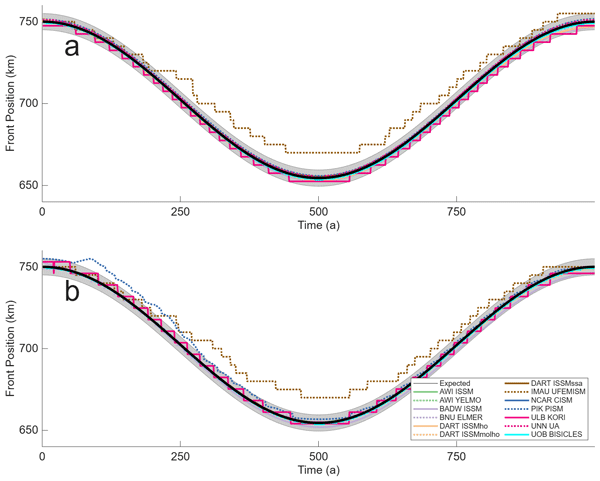
The evolution of the calving front position in time for the Circular domain is shown in Fig. 3 along with a target envelope of 5 km (one grid cell on the common results grid) deviation from the expected position. Out of 13 models, 12 are within the target envelope for the full duration of the run for Profile A (Orthogonal to results grid orientation) whilst 11 are within the envelope for Profile B (Diagonal to results grid orientation). IMAU UFEMISM falls short of the expected amount of total retreat, approximately 10 km outside the target envelope after 500 years and approaching 100 km of expected total retreat. IMAU UFEMISM is symmetric with this offset in both the retreat and advance stage, finishing the simulation with a position very similar to their initial position. A possible explanation for this discrepancy with the expected results is the comparatively low resolution of 20 km used in the IMAU UFEMISM simulations combined with estimating the front position via the fractional area of calving front elements. PIK PISM shows a reduced rate of retreat for Profile B falling outside the envelope for the first 250 years of simulation whilst for the remaining 750 years of the simulation the front position falls within the envelope (Fig. 3b). In the case of PIK PISM, this is most likely a result from interpolating the results onto the common results grid, or from the used analysis method of estimating the calving front position along the diagonal by using mean fractional area coverage. Despite KORI ULB providing its front position only to the nearest grid cell on the results grid, and as such its results appear step like, it is able to consistently match the long term target position. There is some evidence for a drift in calving front position when comparing initial and final positions, with most models ending position being offset from their starting position by a non-zero amount. However, this is a rather small amount (in all cases less than the target envelope) when compared to the temporal and spatial scales of the simulation.

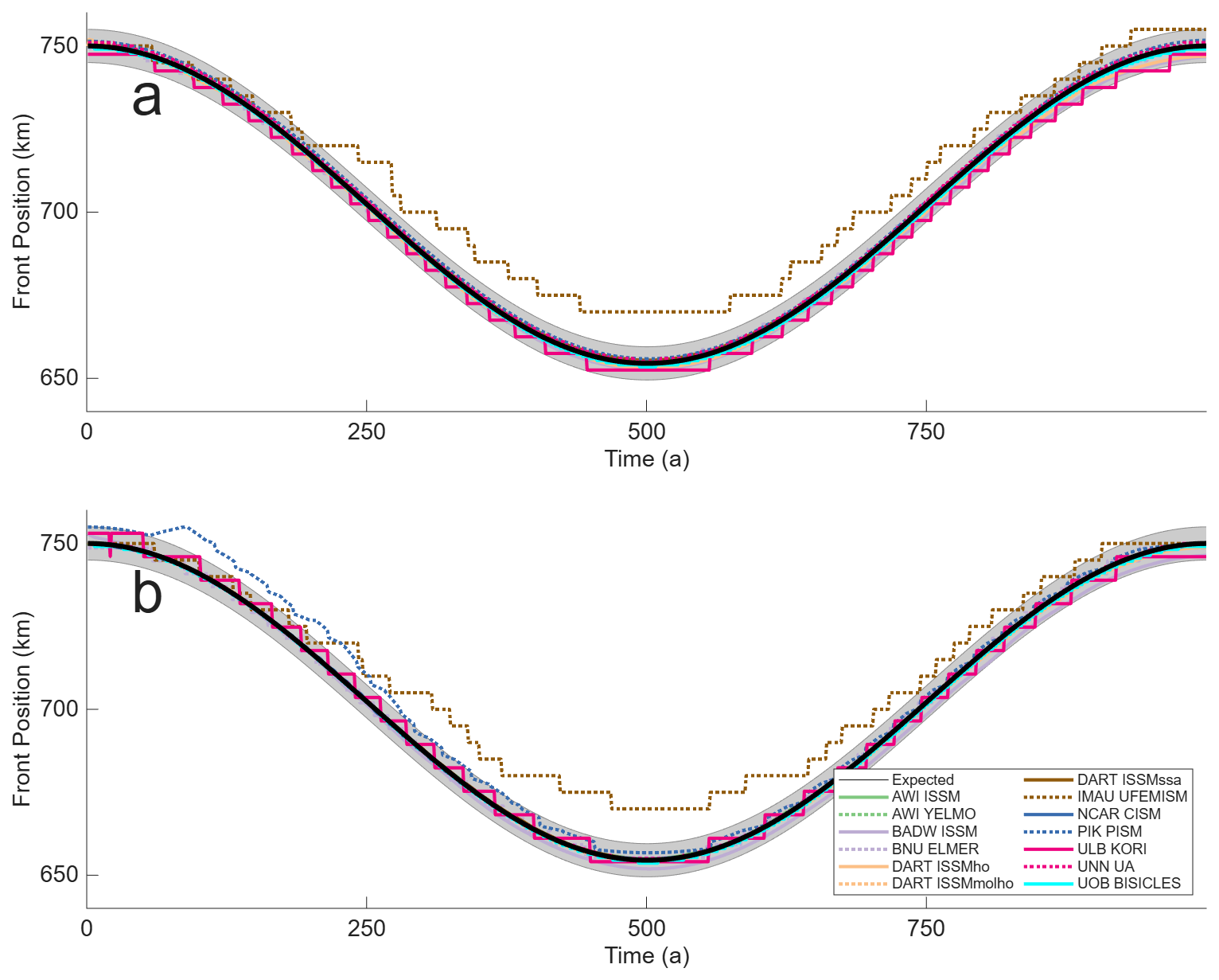
Figure 3 Circular Domain, Calving Front Position. Calving front position over time along Profile A, orthogonal to results grid (a), and Profile B, diagonal to results grid (b). The expected position of the calving front is shown in black, with a target envelope of 5 km, equivalent to one grid cell on the results grid, shown in grey.

4.1.2 Ice properties at the calving front

Ice speed at the calving front is shown in Fig. 4. Note that, as there was no calibration experiment to achieve a target ice velocity, it is not unexpected to observe a certain amount of variation in the absolute values of ice speed between different models even if we would expect a qualitative similarity in the results. The majority of the models display a smooth evolution in ice speed during the calving process with the exception of the AWI YELMO results from diagonal Profile B. During the retreat phase ice velocity simulated by this model frequently oscillates by approximately 25 % of its absolute value, though this is not observed for the advance phase. Models exhibit qualitatively similar absolute values of ice velocity when comparing the two profiles, with ULB KORI showing the greatest change with the front velocity for Profile A 20 m a⁻¹ higher than for Profile B.

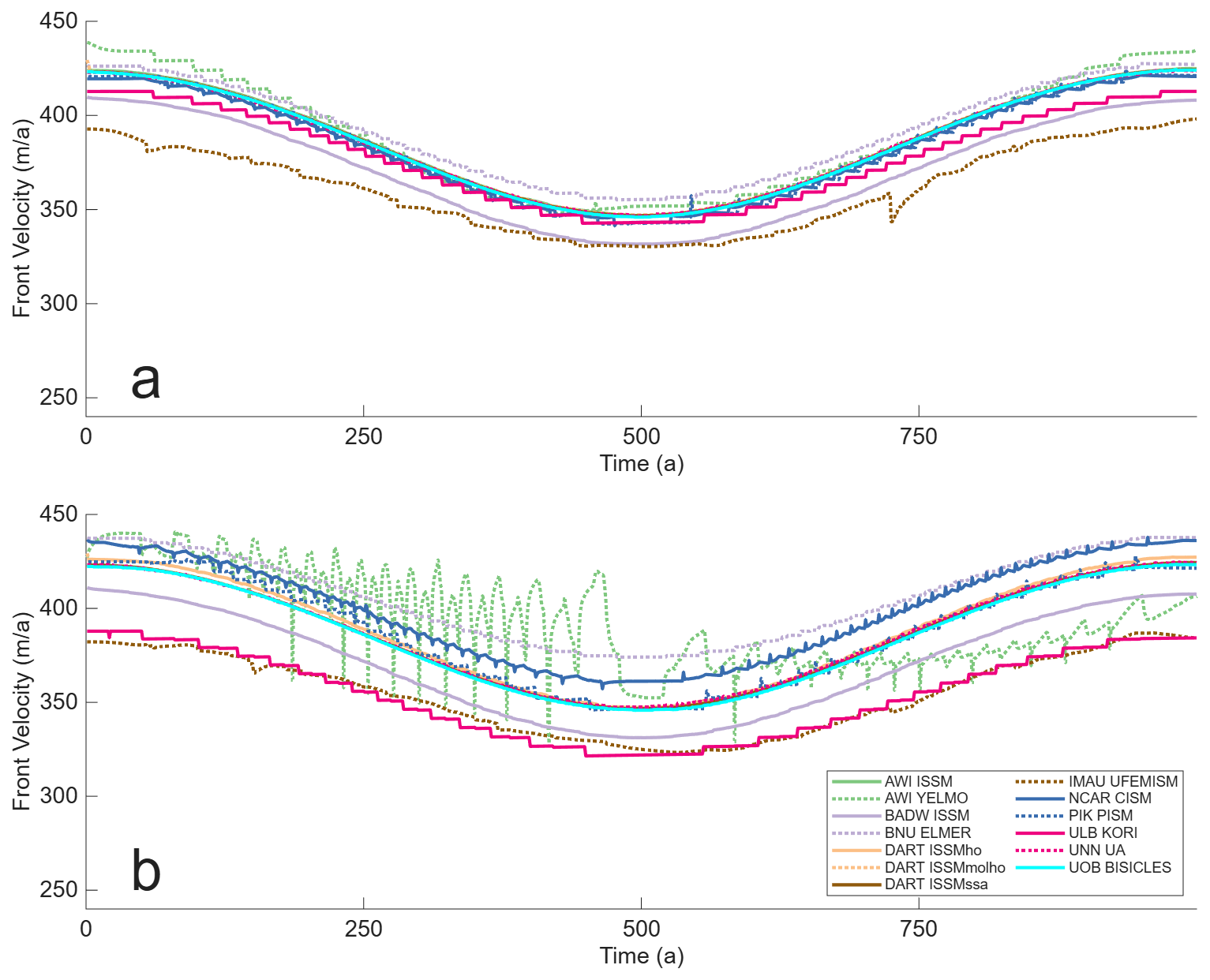
Figure 4 Circular Domain, Calving Front Ice Speed. Calving front ice speed over time along Profile A, orthogonal to results grid (a), and Profile B, diagonal to results grid (b).

Ice thickness at the calving front is shown in Fig. 5. Note that there are no results from IMAU UFEMISM. Similarly as was explained for ice velocity, there was no calibration exercise for ice thickness and so a certain amount of variation between models is to be expected. AWI YELMO shows some noticeable variation during the advance phase of up to 30 % as well as an ice front that is approximately 60 m thinner in Profile B than Profile A. This is most likely results from how the sub-grid scale properties at the calving front are being calculated, as judging from their other results these oscillations in ice properties are contained to the calving front itself. The other models show a smooth evolution of calving front thickness during the simulation, with comparable values of ice thickness in both profiles. Most likely as a result of its slightly greater variation in ice velocity between the two profiles, ULB KORI shows slightly more variation, with an ice front that is 20 m thicker in Profile B than Profile A.

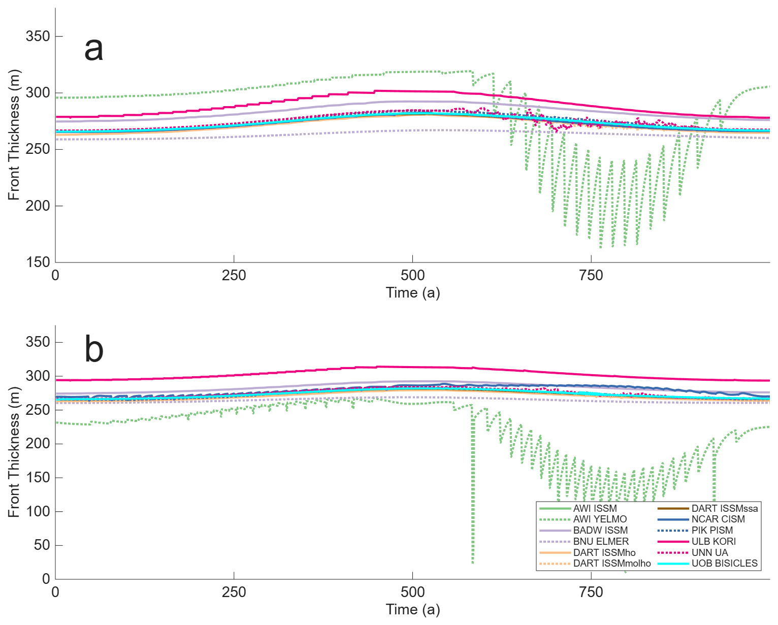
Figure 5 Circular Domain, Calving Front Ice Thickness. Calving front ice thickness over time along Profile A, orthogonal to results grid (a), and Profile B, diagonal to results grid (b).

4.1.3 Model symmetry

The relative area of the four model domain quadrants are shown in Fig. 6. A high degree of symmetry is observed for the majority of models, with small amounts of constant asymmetry noticed in the BADW ISSM, DART ISSMho, IMAU UFEMISM, and UNN UA simulations. The ULB KORI and AWI YELMO simulation also exhibit some asymmetry but unlike the other models this is not a constant amount but changes throughout the run, implying the calving process may be a contributing factor. There does not appear to be a consistent relationship between which models show a higher degree of asymmetry and their use of a regular grid or anisotopric mesh. In all cases it should be noted that in absolute terms there is a very low amount of asymmetry, with never more than a 0.5 % difference in quadrant area observed.

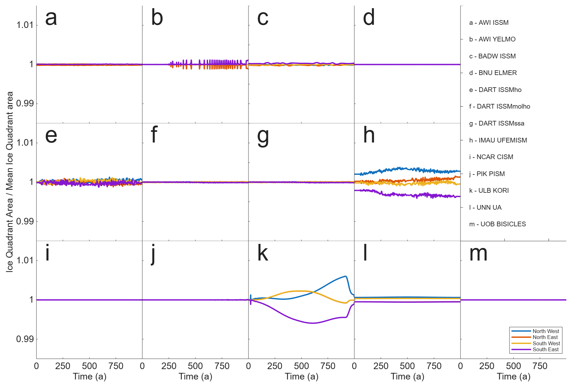
Figure 6 Circular Domain, total ice area by model quadrant. Total ice area for each quadrant of the circular domain relative to quadrant mean total ice area over time.

4.1.4 Ice area and flotation

The relative changes in total, floating and grounded ice area for the circular domain during the simulations are shown in Fig. 7. In the circular domain configuration, calving is taking place into “passive” ice that provides limited additional buttressing. This leads to a high degree of similarity between changes in the total ice area (Fig. 7a) and the floating ice area (Fig. 7b). As such the modelled changes in floating ice have a minimum impact on the grounded part of the domain (Fig. 7c). A small, non zero drift in grounded area is seen for most models, though this is most likely a result of model initialisations not being in a perfect steady state. In line with the reduced rate of retreat shown by IMAU UFEMISM (Fig. 3) it shows less change in floating ice area throughout the simulation.

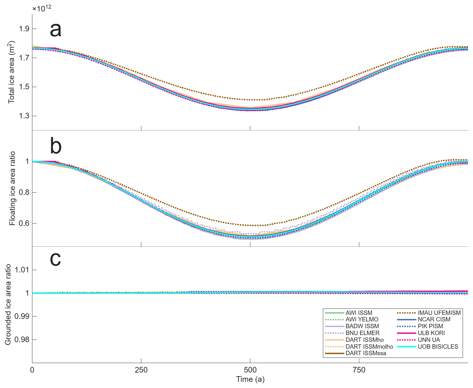
Figure 7 Circular Domain, ice area over time. Total ice area (a), ratio of floating ice area relative to initial floating ice area (b), ratio of grounded ice area relative to initial grounded ice area (c).

Figure 8 shows modelled ice area and thickness relative to the mean thickness for all models at the minimum calving front extent after 500 years of simulated time. Qualitatively, there is a very high degree of similarity for grounded ice, with more variation apparent in the floating ice, with thickness typically varying between ±10 %. BNU ELMER is noticeably thinner, with floating ice up to 20 % thinner than the model mean, however at the calving front itself the ice thickness becomes much closer to the model mean (Fig. 5). ULB KORI has floating ice up to 20 % above the model mean, although with noticeable spatial variability. This is most likely responsible for the relative higher asymmetry for ULB KORI shown in Fig. 6.

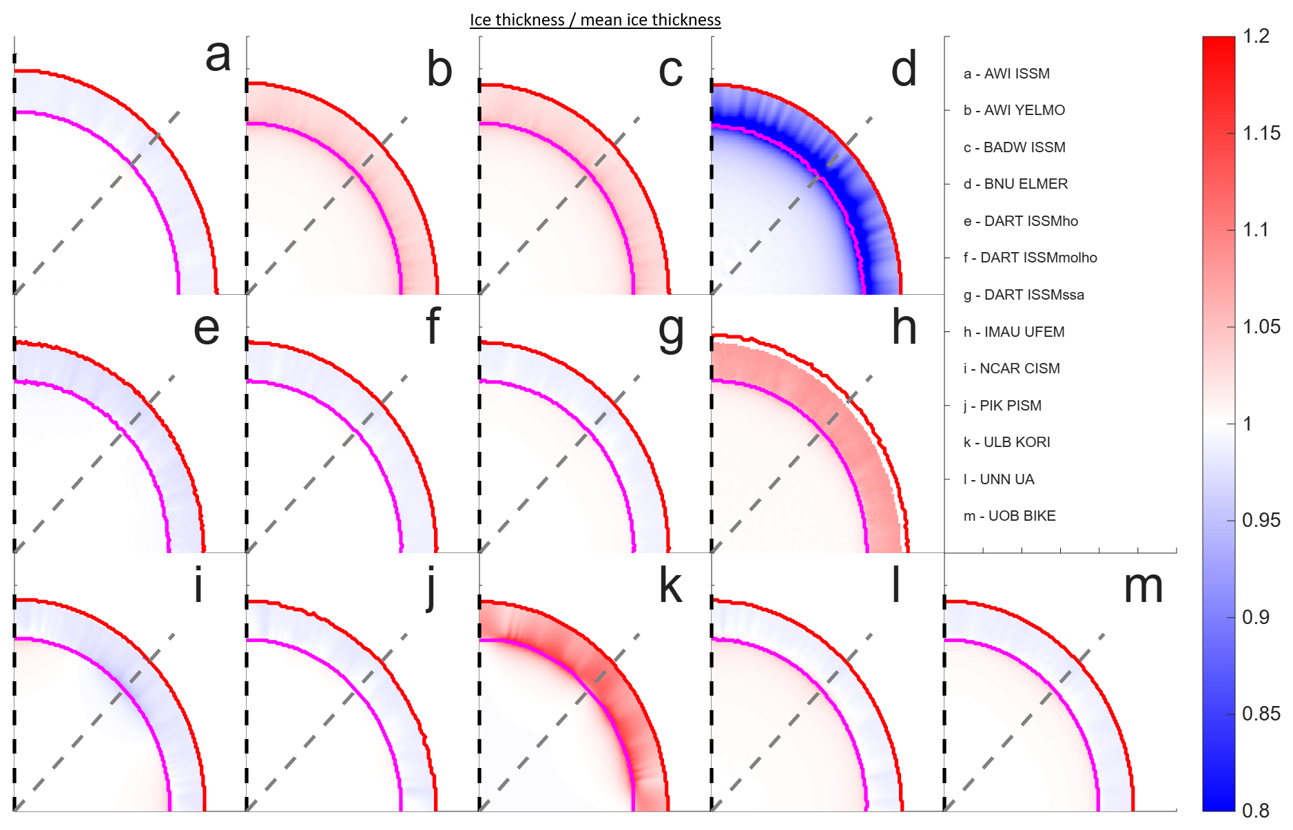
Figure 8 Circular Domain, ice thickness divided by mean ice thickness from all participating models at maximum retreat. Ice thickness after 500 years of run time, with grounding line in magenta and calving front in red. Profile A is shown by the black dashed line, profile B the grey dashed line.

4.2 Thule Domain

4.2.1 Evolution of calving front position

The evolution of the calving front position in time for the Caprona Ice Shelf is shown in Fig. 9a. Whilst there is no a priori solution for the position of the calving front (unlike with the circular domain) there is an initial agreement amongst most of the models, although significantly less so as the simulation progresses and when compared to the circular domain. IMAU UFEMISM stands out from this grouping, with noticeably reduced rates of both retreat and advance, similar to its results in the Circular domain. PIK PISM shows a sudden acceleration in retreat when compared to other models after 350 years, a behaviour which is not seen in the other models. A possible explanation for this is the common result profile interacting poorly with the method used for converting a fractional area on a regular grid into a subgrid scale front position.

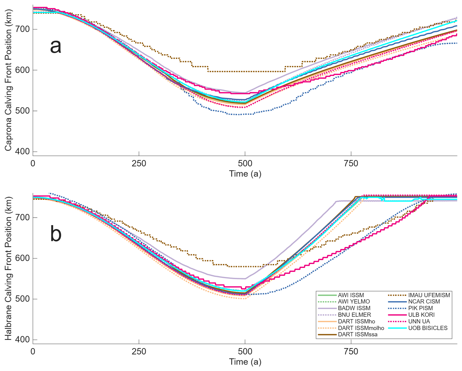
Figure 9 Thule Domain, Calving Front Position. Calving front position over time along Caprona A profile (a) and Halbrane A profile (b).

Figure 9b shows a similar pattern for the Halbrane Ice Stream, with most models grouped together except for IMAU UFEMISM and BADW ISSM both retreating and advancing at a slower rate than the majority. Most models show a linear rate of position change in the second 500 years of the simulation in contrast to the sinusoidal rate of retreat during the first 500 years. Note that a deliberate choice was made in the experimental design to not specify the rate of advance during the second 500 years of simulation so as not to cause an unphysical situation where the calving front advances faster than the ice velocities at the calving front. As such, the rate of advance is highly dependent on the velocity of ice at the calving front and not necessarily due to differences in the calving algorithm.

4.2.2 Ice properties at the calving front

Ice speed at the calving front for Caprona Ice Shelf is shown in Fig. 10a. There is a greater spread and variation of results than was seen for the evolution of the front position (and significantly more than during the circular domain), with the majority of models front-speed increasing as it retreats before decreasing as it advances in the second half of the simulation. It should be noted that, unlike in the circular domain, the results profile is not necessarily orientated in the same direct as ice front velocity, potentially allowing for more variation in results due to how each model implements subgrid scale interpolation. IMAU UFEMISM shows minimal change in front speed throughout the simulation, whilst ULB KORI is the only model to show ice-front speed reduce as the front retreats before speeding up as it advances. Some, though not all, models show more prominent oscillations in ice speed when compared to the circular domain results. These are still fairly minor in the absolute sense, limited to at maximum 5 % of the front speed. Front speed at Halbrane Ice Shelf (Fig. 10b) show a qualitatively similar amount of variation to Caprona ice shelf, with significantly more than the circular domain. The general trend shows ice front speed fall as the ice front retreats and then mostly level off after 250 years. PIK PISM goes against this trend, with an increase in ice-front speed observed after 250 years. AWI YELMO and IMAU UFEMISM show a relatively sudden drop in calving front speed during the advance phase that is not seen in other models.

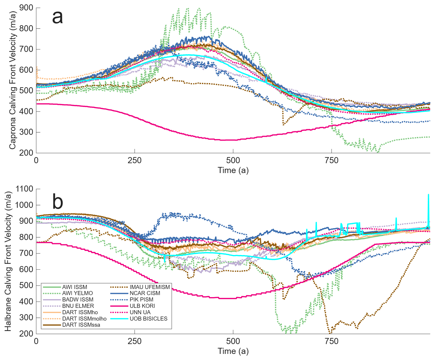
Figure 10 Thule Domain, Calving Front Ice Speed. Calving front ice speed over time along Caprona A profile (a) and Halbrane A profile (b).

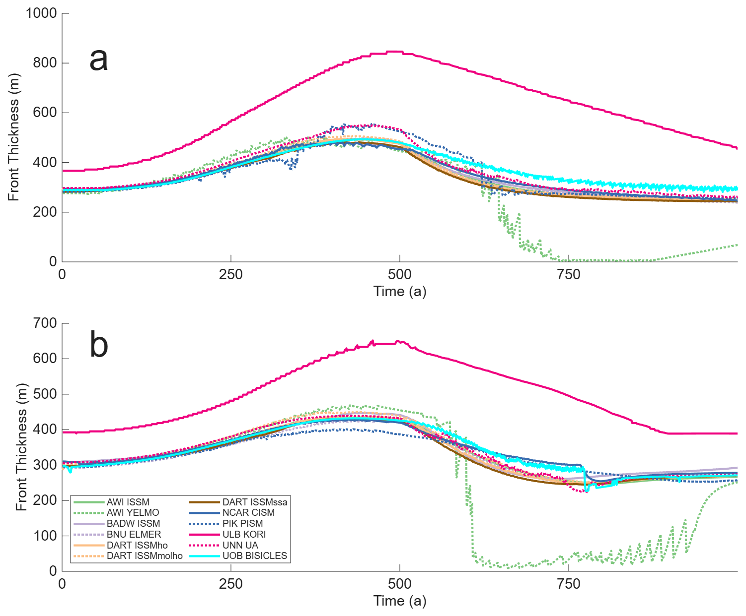
Figure 11 Thule Domain, Calving Front Ice Thickness. Calving front ice thickness over time along Caprona A profile (a) amd Halbrane A profile (b).

Ice front thickness for the Caprona (Fig. 11a) and Halbrane (Fig. 11b) Ice Shelf evolves in a similar pattern, with the front thickening as the ice retreats. Note that, as in the circular domain, there are no results from IMAU UFEMISM. AWI YELMO shows a significant amount of thickness asymmetry, with the advancing calving front up to 300 m thinner than the retreating calving front. This is most likely results from how the sub-grid scale properties at the calving front are being calculated, as judging from their other results these oscillations in ice properties are contained to the calving front itself.

4.2.3 Model symmetry

The relative area of the four quadrants of the Thule domain are shown in Fig. 12. Slightly more asymmetry is observed when the results are compared to the circular domain, though it should be noted that even the most asymmetrical domains, such as DARTho ISSM are varying by less than 0.05 %. The one exception to this is ULB KORI, which undergoes a spike in model asymmetry after 600 years, with values increasing up to a 20 % difference in quadrant ice area (note the different scale for ULB KORI in Fig. 12k). This persists for approximately 100 years before model symmetry returns to values that are similar to other models. As this is not reflected in other results from ULB KORI it is assumed to be a post processing error.

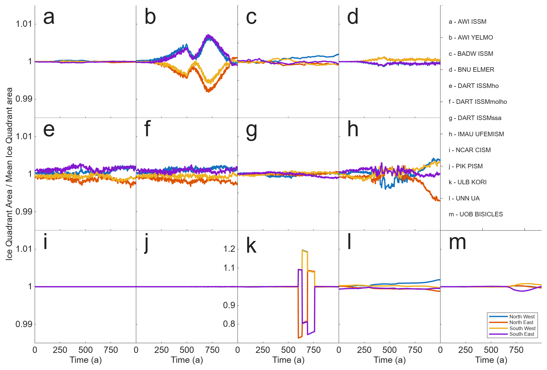
Figure 12 Thule Domain, total ice area by model quadrant. Total ice area for each quadrant of the Thule domain relative to quadrant mean total ice area over time. Note that subplot (k) (ULB KORI) has a different y axis than the other subplots.

4.2.4 Ice area and flotation

The relative changes in total, floating and grounded ice area for the Thule domain during the simulations are shown in Fig. 13. Total ice area is broadly consistent between models at maximum retreat with the exception of ULB KORI and IMAU UFEMISM simulating 10 % increased and PIK PISM 10 % reduced total ice area (Fig. 13a). The majority of models see roughly a 70 % reduction in floating ice area at maximum front retreat (Fig. 13b). IMAU UFEMISM shows less reduction in floating ice area, in line with its results in the circular domain. Most models show at most a reduction of 5 % in total grounded area (Fig. 13c). ULB KORI shows no change in grounded area, whilst PIK PISM is the only model to show a large reduction in grounded area, with the total ice area falling to 85 % of its initial value at maximum retreat. This is most likely a result of ULB KORI generally having thicker than average ice and PIK PISM thinner than the average (Fig. 14).

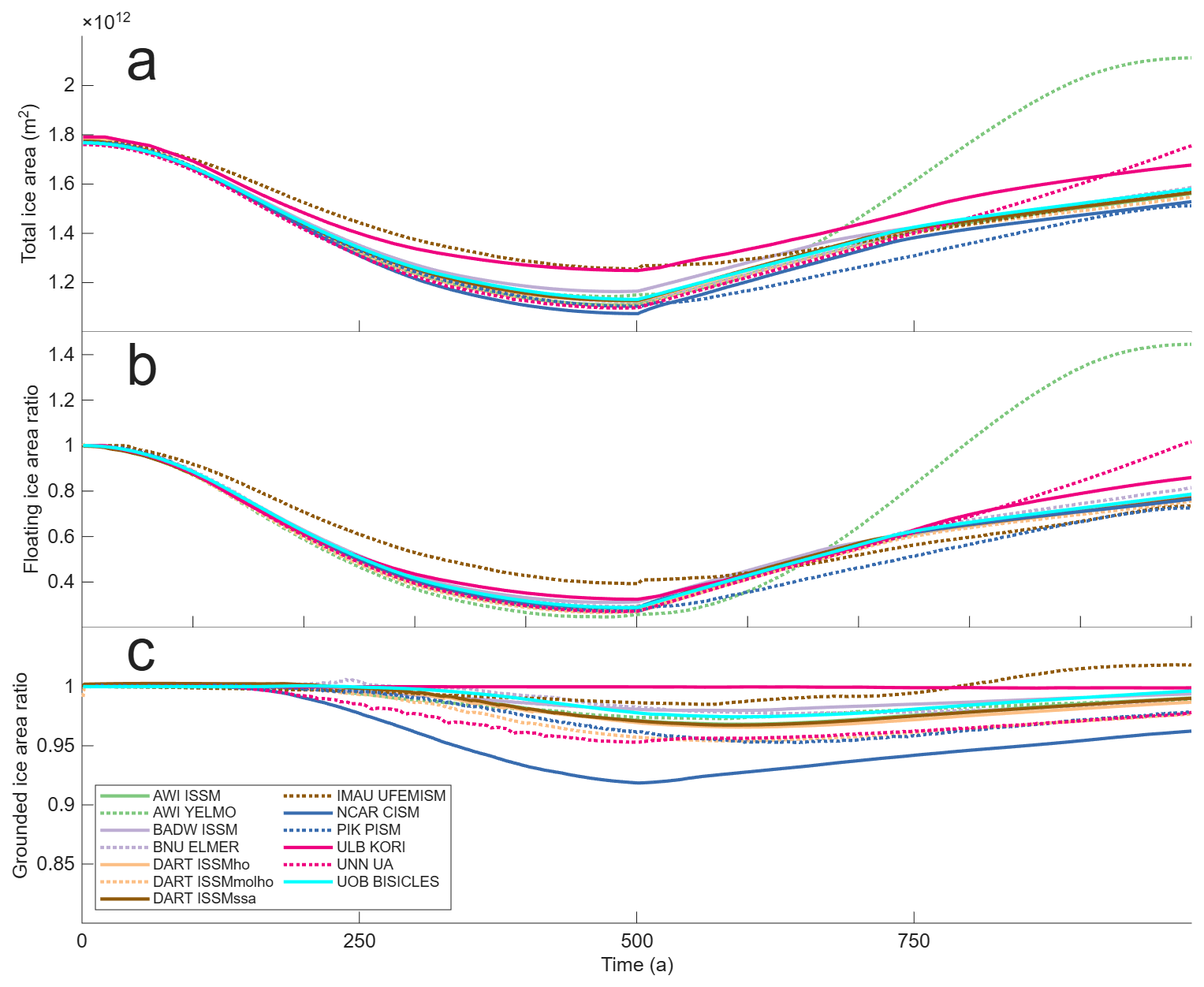
Figure 13 Thule Domain, ice area over time. Total ice area (a), ratio of floating ice area relative to initial floating ice area (b), ratio of grounded ice area relative to initial grounded ice area (c).

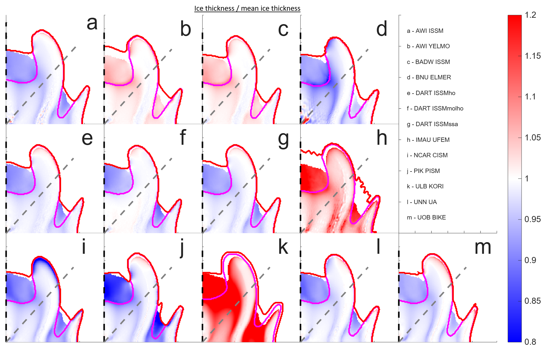
Figure 14 Thule Domain, ice thickness divided by mean ice thickness from all participating models at maximum retreat. Ice thickness after 500 years of run time, with grounding line in magenta and calving front in red. Halbrane profile B is shown by the grey dashed line, Caprona profile B the black dashed line.

Figure 14 shows modelled ice area and thickness relative to the mean of all models at the minimum calving front extent after 500 years of simulated time. Similar to the Circular domain there is a greater variation in ice thickness for floating ice when compared to grounded ice, although unlike the circular domain there is now noticeable variation in the grounded ice thickness. This is most likely a result of the change in buttressing strength provided by varying floating ice thickness impacting grounded ice. As before, thickness varies by up to ±20 % with ULB KORI and IMAU UFEM being noticeably thicker than the average and PIK PISM relatively thinner.

There is a qualitative similarity in total ice front extent between most models, with a couple of exceptions. BNU ELMER, PIK PISM and UOB BISICLES have the western side of Caprona Ice Shelf being noticeably less retreated than the eastern (the ice shelf in the PIK PISM case is actually starting to detach from the grounded ice in this location). There is a noticeable kink in the Halbrane calving front for PIK PISM, with its inflection point occurring close to the results profile line. A smaller kink is noticed in DART-ISSMssa, although further away from the line profile.

5 Discussion

One of the main benefits from undertaking a model intercomparison project that is not always demonstrated to its full effect in the results is the ongoing improvement and optimisation to model implementation and methods that occurs whilst undertaking the required work. Some, but by no means all, examples of this include UNN UA implementing a shock capture scheme to minimise oscillations in ice thickness at the calving front, PIK PISM updating their calving algorithm to incorporate a calving rate as a vector and IMAU UFEMISM had some initial problems determining ice thickness, H, with a moving ice front in a fractional area approach due to the multiple realisations of H(t+dt) needed to determine an implicit solution. Fixing this problem is ongoing work for the IMAU UFEMISM team. Whilst undertaking the work for this project most models significantly improved their results from those initially submitted, both in terms of accuracy as well as spotting previously unnoticed errors in their code. CalvingMIP is not unique in doing this, Model Intercomparison Projects have long been of tremendous benefit to the community by providing the incentive to challenge and test our assumptions about the code we are using (Huybrechts and Payne, 1996). The calving algorithms demonstrated here are all still in active development, with the results here showcasing a snapshot in time of their capabilities.

The calving framework envisioned by CalvingMIP specifies that models should be able to accurately apply a given rate of calving, that ice properties at the calving front should evolve smoothly, that results should be independent of grid orientation, and that the impact of calving on overall ice extent, grounding line position and the ratio between floating and grounded ice is of crucial importance. It is critical that we have confidence that our calving algorithms can address these issues before implementing calving laws in future projections. Our results for the circular domain indicate that the majority of models are able to apply a given calving rate with a high degree of accuracy, have a smoothly evolving calving front in terms of ice thickness and speed, and have their results be mostly independent of model orientation. A slight exception to this is IMAU UFEMISM retreating and advancing not as far as specified with a high degree of ice thickness oscillation at the calving front and AWI YELMO showing significant thickness asymmetry between its advance and retreat phases. Results with more complex bathymetry in the Thule domain show an increasing amount of variation within the simulations. This has the potential to increase further with real world bathymetry, and trying to understand the impact of this variation on predictive models is a key area for future research. However, the overall trend of results show calving algorithms that are ready to accurately and reliably implement calving rates that are generated by separate calving laws, albeit with a few caveats.

Some models (AWI YELMO, PIK PISM, IMAU UFEMISM) have attributed some of the variation in their results to the interpolation method used to determine front properties. As the rate of retreat imposed in our experiments is independent of modelled properties at the calving this should have had minimal impact on how the front position evolves in a simplified domain (Fig. 3), even if it is possibly responsible for oscillations in ice speed and thickness at the calving front. This is likely to have a significant impact on results once models generate their own calving rates via modelled ice front properties and a calving law.

Participating models have taken two different approaches to implementing a calving algorithm, namely either by using a level set function (9 models) or a fractional area approach (4 models, counting UOB BISICLES's pseudo VOF method). At least in regard to the experiments presented here, we find no systematic difference in our results that can be solely attributed to this choice of calving algorithm. Both methods are able to match a given calving rate to a high degree of accuracy and can have qualitatively similar results in terms of calving front properties, etc. Difference between individual models are therefore more likely to be down to precisely how these methods have been implemented into models or from interpolating results from their native grids or meshes to the common regular 5 km results grid rather than due to the choice of calving algorithm. Due to the nature of our experimental design and focus, we have not explicitly tested these approaches with large scale, discrete calving events occurring over a single time step (for example, calving 100 km of ice in a single time step). It is possible that there may be a loss of accuracy or other unforeseen issues if these algorithms are used in such a fashion, though it should be noted doing so was not their initial intended use case. We also find minimal difference in results between the three different DART ISSM configurations, each using a different stress balance (SSA, Higher order, and MOno Layer higher Order), with the exception of slightly more asymmetric results in both the circular and Thule domain for DART ISSMho and the Thule domain for DART ISSMmolho. This implies that calving algorithms in other models should also be largely independent of stress balance.

When considering the spatial distribution of the Caprona ice front in the Thule domain some variation was noticed between the models, with some models retreating the ice front preferentially less on the western side. This has the potential to impact the amount of ice shelf buttressing provided in a similar fashion to simulations with laterally varying rates of ocean driven melting (Jordan et al., 2018). BNU ELMER, PIK PISM and UOB BISICLES exhibited the most variation in this fashion and all applied their calving rates in a direction parallel to ice front velocity rather than perpendicular to ice front geometry. However, NCAR CISM and AWI YELMO also apply their calving rates parallel to ice front velocity and do not show this variation in retreat. As such, when considering the choice of direction for applying the calving rate, we find no consistent difference in ice shelf calving front extent that could be attributed solely to this choice. Whilst we can not attribute the variation in ice thickness across the whole domain of our models to ice shelf calving alone, it does highlight the importance of ice shelf buttressing on long term ice sheet behaviour.

The experiments presented here have focussed on the implementation of calving algorithms and have, so far, ignored calving laws. Having confidence in not only a model's capability to calve a given amount of ice but also that we are applying the right calving rate is of crucial importance for the accuracy and reliability of future predictive models of sea level contributions from ice sheets. To that end, the next phase of CalvingMIP will focus on comparing the impact of different calving laws on ice sheet dynamics. We also intend to, if feasible, compare the choice of a continuous or discontinuous approach to calving. The recent developments in stochastic calving (Ambelorun and Robel, 2025; Benn et al., 2026), where calving rate is represented by a probability density function of individual calving events, would be another interesting point of comparison.

6 Conclusions

We present here results from thirteen different numerical ice models performing a common set of simulations investigating calving algorithms. We find that models are able to accurately implement a given rate of calving, that most models demonstrate a smooth transition in ice shelf properties during the calving process and that their results are independent of model grid orientation. In a simplified, circular domain different models perform with a high degree of qualitative similarity, however a greater spread in results is observed in the experiments utilising more complex synthetic ice sheet bedrock bathymetry. We find no systematic difference in our results from using either a level set or fractional area approach calving algorithm and no discernable difference between applying calving rates perpendicular to ice front geometry or parallel to ice front velocity. Taken together, our results show that we can have a high degree of confidence in the current capability of numerical ice models ability to simulate a given calving rate.