Observational data and neural network-accelerated modelling provide valuable insights for glacier thickness reconstruction in High Mountain Asia

Mountain glaciers provide an irreplaceable water resource in High Mountain Asia, with a significant proportion of water input to rivers coming from glacial meltwater. However, the volume of water held in these glaciers and their evolution over the coming decades is subject to great uncertainty. The reliability of existing glacier ice thickness estimates in High Mountain Asia is limited by the use of low-order models, known to be locally unreliable on mountain glaciers, to describe the relationship between ice velocity and thickness, and by the scarcity of measured thicknesses available for constraint and validation at the time those estimates were produced. We use the Instructed Glacier Model (v2.2.3), a deep-learning-based high-order ice flow model with the capability to invert observed glacier surface velocity for ice thickness, to construct an estimated thickness map of Bhote Kosi glacier. Our thickness inversion is constrained using data collected via a novel airborne radar method for measuring ice thickness. We perform an in-depth case study, carefully justifying inversion parameter choices and quantifying the accuracy of our results. We demonstrate that in the absence of thickness observations, results can be optimized via the use of an L-curve to select the regularization parameter, with significant bias in the unconstrained results, but comparable accuracy to leading thickness estimates. We find that while thickness-constrained inversions are able to correct the modelled thickness field where there is limited information from observed surface velocity, cross-validation experiments demonstrate that the “interpolative power” of thickness observations is weak.

1 Introduction

Forecasting the future evolution of glaciers is vital to predict the volume of ice left in the future, the potential rise in sea level caused by glacier mass loss, and the likelihood of natural hazards such as glacial lake outburst floods (Nie et al., 2021). Even though the world's glaciers contain considerably less mass than the Greenland and Antarctic ice sheets (Farinotti et al., 2019; Morlighem et al., 2017; Pritchard et al., 2025), in recent years they have been responding faster to climate change, with a greater total mass loss than each of the ice sheets individually (Hugonnet et al., 2021). The total mass of glaciers worldwide is predicted to decrease by approximately one quarter to one half in the period 2015–2100, depending on global mean temperature increase (Rounce et al., 2023).

The High Mountain Asia (hereafter abbreviated to HMA) region covers a large area, from the Tian Shan and Hindu Kush mountains in the west to the Himalaya in the east. Leading estimates are clear that the region contains more ice than any other region on Earth outside the polar regions, but there is still significant uncertainty about the quantity of water held in HMA's glaciers (Farinotti et al., 2019; Millan et al., 2022). It has been estimated that glaciers in HMA have been responsible for around 8 %–10 % of total worldwide glacier mass loss in the early twenty-first century (Wouters et al., 2019; Hugonnet et al., 2021; Jakob and Gourmelen, 2023). Rounce et al. (2020) predicts that HMA glaciers are expected to continue to lose a substantial proportion of their mass by 2100, although future glacier mass loss in HMA is hard to quantify with certainty, due to uncertainty in both the future climate and the models used. Of particular concern is the impact on HMA's water resources, as glaciers in the region act as a water reserve that protects rivers and downstream populations from drought. Many rivers in the region receive a large proportion of their input from glacial meltwater, and may lose this input over the coming decades, transitioning (perhaps abruptly) from a glacier-melt-buffered “glacio-pluvial” regime to a mostly pluvial regime dependent on recent precipitation. An estimated 800 million people in the region are dependent in part on the water supply from these rivers (Pritchard, 2019).

With an estimate of the total volume or equivalent mass of water held within a set of glaciers, various glaciological and hydrological questions can be addressed. Potential future sea level rise attributed to a region's glaciers can be quantified from their estimated total mass (Farinotti et al., 2019; Millan et al., 2022). Particularly relevant for HMA is that information about glacier mass and mass loss can aid in making predictions about flooding and future water supply (Pritchard, 2019; Nie et al., 2021).

Additionally, knowledge of thickness distribution (as opposed to total volume) of a glacier is a necessary initial condition for glacier evolution modelling, whereby the future shape and size of a glacier is estimated. Unlike other variables which can be derived from satellite data (such as glacier extent, surface velocity, and change in surface elevation), there is no spaceborne option for measuring ice thickness. Direct measurement of ice thickness can only be obtained through survey in close proximity, with either ground-based or airborne methods. Among the many factors limiting the scope of glacier ice thickness measurement field campaigns are time, monetary cost, equipment available, terrain, altitude, weather, and political constraints. Due to these limitations, glacier ice thickness observations in all regions are generally sparse in both space and time. Accurate estimation of ice thickness distribution is therefore a common, yet unresolved problem in glaciology.

Historically, HMA glaciers have had particularly poor observational coverage, with only 88 out of more than 95 000 glaciers having a thickness measurement in the worldwide Glacier Thickness Database (GlaThiDa), compared with, for example, 175 out of less than 4000 glaciers in Central Europe (Welty et al., 2020). This is partially because glaciers in the region are often debris-covered and have rough surfaces with significant crevassing, making ground-based surveys difficult to carry out. Airborne surveys are able to survey these glaciers more efficiently, but the debris cover and narrow valleys in which these glaciers are found still cause challenges for measuring the ice with radar equipment.

Pritchard et al. (2026) present thickness observations for 13 glaciers (as outlined by RGI Consortium, 2017) in the Himalaya region near Everest, via the use of a bespoke airborne radar system deployed by helicopter and developed specially for use in the region. The increased manoeuvrability of helicopters at high altitude (versus that of fixed-wing aircraft, such as those typically used for thickness surveys of the polar ice sheets) is what made this study possible. Additionally, the use of a low-frequency radar allowed for better penetration into the ice in this region, which is typically covered with debris and has a high water content. This study approximately doubled the combined length of all surveyed thickness profiles in the entire HMA region, opening up new possibilities for calibration and validation of thickness estimates.

Ice thickness estimation (often termed thickness “inversion”) has become considerably more tractable in recent years due to the increase in quality and availability of satellite data. The first worldwide glacier thickness estimation study was performed by Huss and Farinotti (2012), based on mass conservation principles and without using any information about the surface velocity. Satellite-observed surface velocity data is now available for glaciers worldwide (Millan et al., 2022; Gardner et al., 2025), and is a prerequisite for many ice thickness estimation methods (Farinotti et al., 2017). Change in surface elevation is another satellite-derived data product that is required for many of the thickness estimation methods based on mass conservation (Farinotti et al., 2017), and has been mapped for glaciers worldwide by Hugonnet et al. (2021). One challenge that persists in the estimation of ice thickness is the sparsity and paucity of available thickness observations for validation (Welty et al., 2020).

The first phase of the Ice Thickness Models Intercomparison eXperiment (ITMIX, Farinotti et al., 2017) focused on glacier ice thickness estimation methods which do not use thickness observations at all to compute their thickness estimate. They found that thickness estimates vary depending on method, and that averaging the results of several methods is a viable strategy to obtain an accurate result. The second phase of ITMIX (ITMIX2, Farinotti et al., 2021), on the other hand, focused on validation of models which do calibrate to available thickness observations. ITMIX2 performed experiments where various subsets of the available thickness profiles were removed from the calibration, and the error of the resulting thickness field was then evaluated against the removed profiles. In the statistics and machine learning fields, this technique is known as cross-validation (Picard and Cook, 1984). The results of these experiments demonstrated that even limited sets of thickness observations are effective for reducing model bias (i.e. constraining volume), and that the spatial distribution of thickness observations has a weak effect on the quality of estimates.

Farinotti et al. (2019) averaged the results of several different methods to obtain a “consensus” estimate, based on the findings from Farinotti et al. (2017). Millan et al. (2022) produced thickness estimates for glaciers worldwide by taking advantage of a high-resolution surface velocity dataset, directly inverting the shallow ice approximation (SIA) to obtain a simple relation between thickness and surface velocity. The results of Farinotti et al. (2019) and Millan et al. (2022) are currently widely used by the glacier modelling community, with several studies building on these results (e.g. Immerzeel et al., 2020; Sommer et al., 2020; Khanal et al., 2021; Zheng et al., 2021; Bosson et al., 2023; Zekollari et al., 2024). Hereafter we refer to the thickness estimates of Farinotti et al. (2019) and Millan et al. (2022) as the “consensus” estimate and “Millan” estimate respectively.

Other glacier and ice sheet inversion studies focus on attempting to estimate physical parameters related to basal sliding from observed velocities, often using adjoint methods, which are not limited to the SIA, but require lengthy manual derivation (MacAyeal, 1992; Goldberg and Heimbach, 2013). Recent advances in the field of machine learning, including automatic differentiation and optimization libraries such as Tensorflow (Abadi et al., 2015) and Keras (Chollet, 2015), as well as the development of new optimizers based on stochastic gradient descent (e.g. Kingma and Ba, 2017), have opened up new possibilites for solving inverse problems in glaciology. Steidl et al. (2025) constructed a physics-informed neural network, based on mass conservation, to estimate the thickness of glaciers in Svalbard. Maffezzoli et al. (2025) used gradient-boosted trees, another machine learning technique, to estimate the thickness of glaciers worldwide, with error comparable to the consensus and Millan estimates. Schmitt et al. (2026) presented a time-dependent inversion method which aims to create a dynamically consistent initialization of a glacier using the 4DVar data assimilation technique and automatic differentiation.

The Instructed Glacier Model (Jouvet and Cordonnier, 2023), hereafter abbreviated as IGM, is a novel deep-learning-based glacier model which has shown promise for both prognostic (forecast) and diagnostic (state estimation) modelling. As an emulator for the Blatter–Pattyn (also known as first-order approximation) equations (Pattyn, 2003), it has been shown to evaluate orders of magnitude faster than traditional Stokes-solving methods, excluding training time (Jouvet et al., 2022), and is equipped with a module that performs ice thickness inversion via a minimization approach (Jouvet, 2023). Cook et al. (2023) used IGM to first estimate current glacier thickness of the entire European Alps, and then to compute forecasts on a short (less than 50 years) time scale, on the basis that using the same physical model for both inversion and forward evolution will help to overcome the initial non-physical effects often experienced by glacier evolution models when modelling over such a short time scale. Frank and van Pelt (2024) and van Pelt and Frank (2025) used IGM for thickness inversion of glaciers in Scandinavia and Svalbard, although only as a forward model, with the authors opting for their own inversion method. The IGM inversion method has also been used for estimating surface mass balance of avalanching glaciers (Kneib et al., 2024).

In this study, we present in-depth analysis of the process of estimating the thickness of a previously unmeasured glacier in the Himalaya region. We use and scrutinize an inversion method based on cost minimization, making careful and methodical choices regarding the inversion parameters. We first investigate how well ice thickness can be reconstructed with knowledge of ice surface velocity alone, using the L-curve technique (Hansen and O'Leary, 1993) to find an optimal value for a key inversion meta-parameter. We use recently reported thickness observations from Pritchard et al. (2026) to validate our estimate, and compare our results with the Millan estimate. Then, we introduce the thickness data for calibration of the ice thickness, performing cross-validation experiments to assess the influence of spatial distribution of thickness observations. We demonstrate that parameter choices can strongly influence results, and consider the value added by an entirely new dataset of thickness observations.

2 Model, data, and methodology

Our thickness inversion is based on the method described in Jouvet (2023). This method relies on an ice-flow model emulator in the form of a convolutional neural network (CNN), as described in Jouvet and Cordonnier (2023), implemented in the framework of the IGM. The emulator's role is to replace the solving of the Blatter–Pattyn equations (Pattyn, 2003) for the three-dimensional velocity field, given the shape of the glacier and parameters representing the viscosity and basal sliding. IGM is also equipped with an inversion module, whose purpose is to estimate unknown variables based on available observational data, using the emulator as a forward model. In this section we summarise the inversion algorithm and outline our methodology for a detailed case study on one glacier in the Himalaya region.

2.1 Instructed Glacier Model

The IGM emulator is a CNN that takes as input two-dimensional arrays of glacier thickness h, surface topography s, Arrhenius factor A (a number that determines the ice viscosity; Glen, 1953), and a sliding coefficient c (based on a Weertman sliding law; Schoof and Hewitt, 2013), and outputs both horizontal velocity components u,v as three-dimensional arrays (Jouvet and Cordonnier, 2023, Fig. 3). All variables are defined over a rectangular domain Ω, and on a structured uniform orthogonal axis-aligned grid with cell width H. Each input array has dimensions N_x×N_y (width times height of the domain Ω in terms of number of cells), and each output array has dimensions $N_x\times N_y\times N_z$, where N_z represents the number of vertical layers. The neural network can be represented as follows, where the subscript (⋅)_H denotes the discretized variable:

$$\begin{array}{}\text{(1)}& {\displaystyle }{\displaystyle }{\mathcal{N}}_{\mathit{\lambda }}:(h_H,s_H,A_H,c_H){\displaystyle }\mapsto (u_H,v_H).\end{array}$$

Hereafter we will drop the subscript (⋅)_H for clarity, with the understanding that all variables are discretized within IGM.

As described in Jouvet and Cordonnier (2023), the weights λ of the CNN are trained to minimise the energy functional associated with the Blatter–Pattyn model (Pattyn, 2003), thereby replacing the solver that would usually be present in a glacier model, and making this method a form of physics-informed neural network (PINN). PINNs are a method of approximating the solution of a differential equation by way of a neural network. PINNs typically take spatial and/or temporal coordinates as input, and incorporate physical laws into their loss function in the form of the residual of a differential equation and its boundary conditions (Raissi et al., 2019). IGM's ice flow emulator differs from the original PINN method in two important ways: the inputs to the neural network are fields defined on the entire horizontal grid, rather than spatial coordinates, and the loss function is the energy functional (similar to the “variational PINN” or “VPINN” described by Kharazmi et al., 2019), not the residual of the equations and boundary conditions. The formulation of the energy functional of the Blatter–Pattyn model is omitted, but can be found elsewhere in the literature (e.g. Jouvet and Cordonnier, 2023; Jouvet, 2016; Schoof, 2006).

We use a pretrained CNN (available from the IGM repository on GitHub), which has the architecture described in Jouvet and Cordonnier (2023): 16 two-dimensional convolutional layers each with a 3×3 kernel and 32 output filters, with padding to conserve the frame size, and leaky rectified linear units as the activation functions, resulting in a CNN with about 140 000 trainable parameters. The CNN has been pretrained on a catalogue of mountain glaciers specifically chosen to be heterogenous and representative of a variety of glacier shapes (Jouvet et al., 2022).

The benefit of the CNN approach over that of traditional ice flow models is that evaluation of the pretrained neural network is fast, especially on a GPU. Additionally, it allows the use of the Blatter–Pattyn model, which for mountain glaciers is more appropriate than the SIA used in the Millan global thickness inversion study.

The encoding of the Blatter–Pattyn model equations as a neural network also makes the inversion framework simple to set up, taking advantage of automatic differentiation, and using tools from the Tensorflow (Abadi et al., 2015) and Keras (Chollet, 2015) Python libraries. The aim of the inversion module in IGM is to invert the ice flow mapping (Eq. 1). We take known surface velocity data, surface topography data, and thickness measurements (where present), and pick some combination of thickness h, surface topography s, Arrhenius factor A, and sliding coefficient c to be control variables which we can adjust. The aim is to obtain an optimal fit of these control variables across the whole glacier, in the sense that the misfit between the surface velocity output from the emulator (Eq. 1) and the observed surface velocity is small (Jouvet, 2023).

In this study, we focus on thickness h as the only control variable. The optimized map is obtained by minimising the cost function

$$\begin{array}{}\text{(2)}& {\displaystyle }{\displaystyle }\mathcal{J}\left(h\right)={\mathcal{C}}^u+{\mathcal{C}}^h+{\mathcal{R}}^h+{\mathcal{P}}^h.\end{array}$$

Letting ℳ denote the ice-covered domain, the misfit between modelled and observed surface velocities is

$$\begin{array}{}\text{(3)}& {\displaystyle }{\displaystyle }{\mathcal{C}}^u={\displaystyle \frac{\mathrm{1}}{\mathrm{2}{\mathit{\sigma }}_u^{\mathrm{2}}}}{\displaystyle \frac{\mathrm{1}}{\text{area}\left(\mathcal{M}\right)}}\underset{\mathcal{M}}{\int }{\left|{\mathit{u}}_s^{\text{obs}}-{\mathcal{N}}_{\mathit{\lambda }}(h,s,A,c)\right|}^{\mathrm{2}}\mathrm{d}m,\end{array}$$

where ${\mathit{u}}_s^{\text{obs}}=(u_s^{\text{obs}},v_s^{\text{obs}})$ denotes the vector field of observed horizontal velocity at the surface and $|\cdot |$ denotes the Euclidean norm. Letting 𝒯⊆ℳ denote the subset of cells for which thickness observations exist, the misfit between modelled and observed ice thickness is

$$\begin{array}{}\text{(4)}& {\displaystyle }{\displaystyle }{\mathcal{C}}^h={\displaystyle \frac{\mathrm{1}}{\mathrm{2}{\mathit{\sigma }}_h^{\mathrm{2}}}}{\displaystyle \frac{\mathrm{1}}{\mathit{\#}\text{cells}\in \mathcal{T}}}\sum _{\text{cells}\in \mathcal{T}}{\left|h-h^{\text{obs}}\right|}^{\mathrm{2}},\end{array}$$

where $|\cdot |$ denotes absolute value. Details of the computation of the discretized h^obs are given in Sect. 2.2.2.

A regularization term is included to minimize the presence of non-physical small-scale spatial variations in the thickness field. Although our control variable is thickness h, we instead regularize the bedrock $b=s-h$ (note that the surface elevation s, which is derived from a DEM, does not change at all in our inversion setup, and that b=s outside ℳ). While the inclusion of this term has the effect of regularizing the ice thickness, it additionally imposes smoothness of the bedrock at the boundary of ℳ. The regularization term for the bedrock elevation is

$$\begin{array}{ll}{\displaystyle }{\mathcal{R}}^h=& {\displaystyle }{\displaystyle \frac{{\mathit{\alpha }}_h}{\mathrm{2}\sqrt{\mathit{\beta }}}}{\displaystyle \frac{\mathrm{1}}{\text{area}\left(\mathrm{\Omega }\right)}}\\ \text{(5)}& {\displaystyle }& {\displaystyle }\times \underset{\mathrm{\Omega }}{\int }\left({\left|\mathrm{\nabla }b\cdot {\stackrel{\mathrm{̃}}{\mathit{u}}}_s^{\text{obs}}\right|}^{\mathrm{2}}+\mathit{\beta }{\left|\mathrm{\nabla }b\cdot {\stackrel{\mathrm{̃}}{\mathit{u}}}_s^{\text{obs},⟂}\right|}^{\mathrm{2}}\right)\mathrm{d}m\end{array}$$

where ${\stackrel{\mathrm{̃}}{\mathit{u}}}_s^{\text{obs}}$ is the observed surface velocity after smoothing with a Gaussian filter with standard deviation 3 and then normalizing, $({\stackrel{\mathrm{̃}}{\mathit{u}}}_s^{\text{obs}}{)}^{⟂}$ is the unit vector field orthogonal to it, and β is a coefficient which allows for anisotropic smoothing (β=1 corresponds to isotropic smoothing, β closer to 0 enforces more smoothing in the along-flow direction). In all of our experiments, we fix the anisotropy factor at β=0.2. The final term is a quadratic penalty term (Nocedal and Wright, 2006, Sect. 17) to enforce non-negative ice thickness and zero thickness outside the ice-covered domain:

$$\begin{array}{ll}{\displaystyle }{\mathcal{P}}^h={\mathrm{10}}^{\mathrm{10}}(& {\displaystyle }{\displaystyle \frac{\mathrm{1}}{\text{area}(\mathrm{\Omega }\setminus \mathcal{M})}}\underset{\mathrm{\Omega }\setminus \mathcal{M}}{\int }{h}^{\mathrm{2}}\mathrm{d}m\\ \text{(6)}& {\displaystyle }& {\displaystyle }+{\displaystyle \frac{\mathrm{1}}{\text{area}(\text{cells where }h<\mathrm{0})}}\underset{h<\mathrm{0}}{\int }{h}^{\mathrm{2}}\mathrm{d}m).\end{array}$$

The parameters σ_u,σ_h are user-defined weights which can be thought of as “confidence levels” for the observed surface velocity and thickness respectively – a lower σ corresponds to more “confidence” and more weight placed on matching these observations. Note that these σ values do not represent measurement error; they are intended to be tuned by the user (Jouvet, 2023). The regularization parameter α_h controls how much weight is placed on smoothing the thickness field.

In this study, the thickness field is initialized with the Millan thickness estimate. A sensitivity test was conducted to confirm that results are independent of the starting point: the ice thickness field was initialized at a constant 100 m inside ℳ and zero elsewhere, and the results were indeed very close to the results obtained by initializing with the Millan thickness. We use the Millan thickness as the initial thickness as it is expected to be relatively close to the solution (compared to a constant 100 m thickness), thereby helping the optimization to converge sooner.

The cost 𝒥(h) is minimized using the Adam optimizer (Kingma and Ba, 2017), which is a popular method for training neural networks, and is a variation on stochastic gradient descent with momentum. The inversion begins with a pretrained neural network 𝒩_λ, which goes through one iteration of retraining (also with Adam) after each inversion iteration, using the current glacier geometry as the training data. The aim of retraining is to keep the neural network loss (the energy functional associated with the Blatter–Pattyn model) low, so that the emulator continues to produce output that is close to Blatter–Pattyn solutions. We used one retraining iteration per inversion iteration (the model default), which is expected to provide sufficient fine-tuning, as the thickness field is expected not to deviate much between inversion iterations, especially later on in the optimization procedure. Examples of how the inversion cost (Eq. 2) and neural network loss evolve over iterations of the optimization algorithm in practice can be found in Appendix A.

We emphasize that it is not necessary for the velocity to be modelled as the output of a neural network: the method of minimizing Eq. (2) would also be possible with an alternative method of finding the velocity, e.g. by directly minimizing the energy functional of the Blatter–Pattyn model to find the solution. Among the benefits of using a neural network emulator are fast evaluation (especially on GPU), differentiability, and the resulting simplicity of the cost function, particularly the velocity component (Eq. 3).

We note also that IGM's inversion module allows for additional control fields and cost terms, as outlined in Jouvet (2023). We opted not to use the surface elevation as a control variable as this would double the degrees of freedom, possibly admitting non-unique solutions. Furthermore, we decided not to use terms constraining the flux divergence, as the options are to either match to observed flux divergence (this would require reliable surface mass balance observations, which are not available for our glacier of interest), or to match to a linear regression of the modelled flux divergence, which is recomputed at every iteration and can reinforce unrealistically high flux divergence values.

2.2 Data

2.2.1 Data acquired through OGGM

To retrieve the required data, we use the built-in framework of IGM, which in turn relies on preprocessed data provided by the Open Global Glacier Model (OGGM) developed by Maussion et al. (2019). OGGM defines a spatial grid for each glacier with a resolution of H=100 m, in a local coordinate reference system (EPSG:32645 – WGS 84/UTM zone 45N). All variables are projected onto this grid.

Glacier outlines and identification numbers are provided by the Randolph Glacier Inventory (RGI) v6.0 (RGI Consortium, 2017). A rasterized mask is created from the outline to define ice-free areas. The digital elevation model (DEM) is that of Copernicus (2019), with acquisition dates between 2010–2015. Surface velocities are those computed by Millan et al. (2022), derived by feature tracking of image pairs acquired by the optical sensors onboard satellites Landsat 8 and Sentinel-2, and the synthetic aperture radar onboard Sentinel-1, between 2017–2018. Finally, to initialize the IGM inversion, we use the ice thickness estimate from Millan et al. (2022), which was derived from the velocity dataset from the same study.

2.2.2 Thickness observations

In addition to the data available through OGGM, we use the thickness observations from Pritchard et al. (2026). These measurements, obtained by airborne ground-penetrating radar in October and November 2019, cover 13 glaciers (as identified in RGI v6.0) near Mount Everest. Further details on the processing of the radar data, as well as error analysis, are available in Pritchard et al. (2026).

The pointwise thickness measurements are provided in a vector (ESRI shapefile) format. In some places, points are as close together as 1 m, while the resolution of our model is 100 m. We rasterize the thickness observations for use in IGM by taking the mean thickness in a 100 m×100 m square centred on each coordinate point in our grid.

We acknowledge that the aggregation of thicknesses in this way does incur a loss of information from the original vector dataset. While it would in theory be possible to compare the modelled thickness field with pointwise thickness measurements, as recommended by Nixon-Hill et al. (2024), this would require refactoring of the IGM code, and we would instead be faced with the question of how to interpolate the modelled thickness field at the observation locations. We opt for rasterization of the thickness dataset, as this is easily implemented within the current IGM framework and a similar approach was taken in Farinotti et al. (2021).

The glacier outlines from RGI v6.0 are intended to represent the state of the glacier in the year 2000 (or as close as possible), and comparison with more recent high-resolution satellite imagery shows that there are cases where an outline may not be representative of the recent state of the glacier. Indeed, when preparing the thickness observation data, it became clear that some thickness observations lie outside RGI v6.0 glacier outlines (see e.g. Fig. B1). For ease of modelling, we prioritise the outlines over the observations, and discard all thickness observations outside the rasterized glacier mask derived from the outline.

2.3 Methodology

Bhote Kosi glacier (whose RGI v6.0 ID is RGI60-15.03422) was chosen for an in-depth study. It is one of the largest glaciers in the Pritchard et al. (2026) dataset and has good coverage of thickness observations, with several longitudinal (along-flow) and across-flow profiles, and observations across a wide elevation range (see Fig. 1). Pritchard et al. (2026) notes that different parts of this glacier are known by different names: Bhote Kosi is the southern main “trunk” of the glacier, with the west tributary and north tributary called Lunag and Nangpa respectively. Throughout this paper we typically use the name Bhote Kosi to refer to the entire glacier, since it is dynamically connected and appears as one glacier in RGI v6.0.

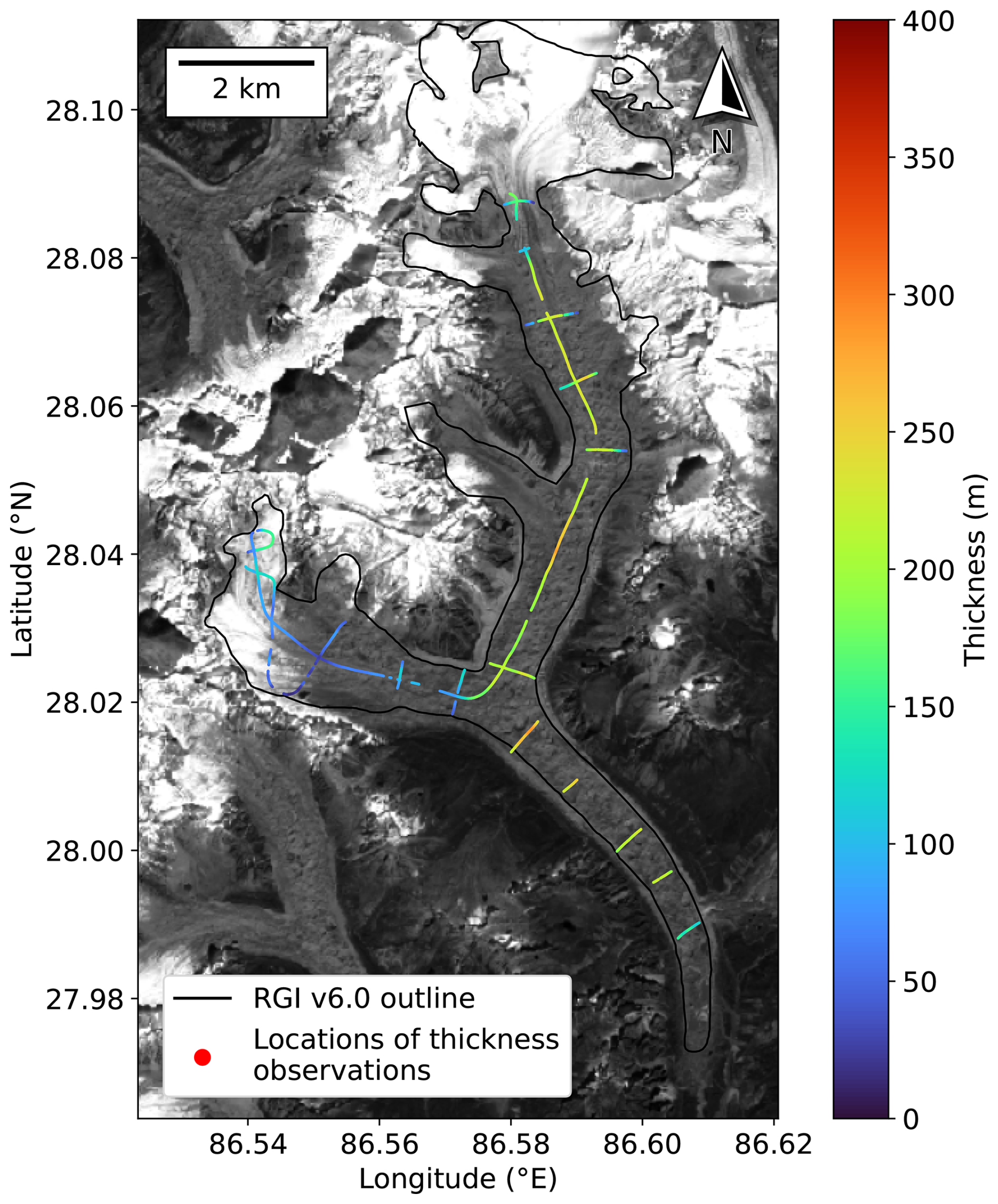
Figure 1 Bhote Kosi glacier (RGI60-15.03422) outline in black. Locations of Pritchard et al. (2026) thickness observations are coloured according to their observed thickness value. Background image is a Sentinel-2 scene (band 04) from 15 October 2019 (contains modified Copernicus Sentinel data [2019] processed by Sentinel Hub). Latitude and longitude coordinates are shown for geographical context.

We perform several thickness inversion experiments on Bhote Kosi glacier, starting with a simple configuration, and progressively introducing more complexity. We begin by performing inversions without calibrating to thickness observations, in order to tune the ratio between σ_u and α_h. We then introduce thickness observations into the inversion, aiming to find an appropriate value for σ_h, and perform cross-validation experiments to explore the value added by calibrating to thickness observations.

Initial experiments with IGM inversion showed that the choice of parameters σ_u, σ_h, and α_h can have a significant effect on the resulting thickness field (see Fig. C1). With our in-depth study on Bhote Kosi, we aim to find a set of parameters that provide an optimal balance between matching observed surface velocities and producing a realistically smooth thickness field.

2.3.1 Error metrics

In each experiment, we measure the error with unseen (validation) thicknesses using two different statistics: the mean absolute error (MAE) and the mean bias error (MBE). The MAE over a set of grid cells 𝒯 with thickness observations is the absolute value of the difference between modelled and observed thickness, averaged over all cells in 𝒯:

$$\begin{array}{}\text{(7)}& {\displaystyle }{\displaystyle }\text{MAE}\left(\mathcal{T}\right)={\displaystyle \frac{\mathrm{1}}{\mathit{\#}\text{cells}\in \mathcal{T}}}\sum _{\text{cells}\in \mathcal{T}}\left|h-h^{\text{obs}}\right|.\end{array}$$

The MBE over a set of grid cells 𝒯 is simply the difference between modelled and observed thickness, averaged over all cells with a thickness observation:

$$\begin{array}{}\text{(8)}& {\displaystyle }{\displaystyle }\text{MBE}\left(\mathcal{T}\right)={\displaystyle \frac{\mathrm{1}}{\mathit{\#}\text{cells}\in \mathcal{T}}}\sum _{\text{cells}\in \mathcal{T}}\left(h-h^{\text{obs}}\right).\end{array}$$

By including the sign of the difference, the MBE has a convenient interpretation: a negative MBE indicates that on average, the model underestimates the ice thickness (and hence the total volume), whereas a positive MBE indicates overestimation. It is desirable for both MAE and MBE to be close to zero.

2.3.2 “Velocity-only” inversion

We begin by matching observed velocities only (the term 𝒞^h is omitted from Eq. 2). Available thickness observations are used only as validation data, i.e. to assess the accuracy of the thickness estimate after the inversion has been performed. We use IGM's default values of A=78 ${\mathrm{MPa}}^{-\mathrm{3}}{\mathrm{yr}}^{-\mathrm{1}}$ for the Arrhenius parameter and c=0.0464 $\mathrm{MPa}{\mathrm{yr}}^{\mathrm{1}/\mathrm{3}}{\mathrm{m}}^{-\mathrm{1}/\mathrm{3}}$ for the sliding coefficient (both are taken to be spatially constant). The velocity-only inversion scheme was run for 18 approximately logarithmically spaced values of α_h between 0.01–60, keeping σ_u=1 fixed (note that we can fix one of the coefficients without loss of generality: multiplying all cost terms by the same factor would not change the locations of minima). For each α_h, the optimization algorithm was run for 1000 iterations, resulting in a different final thickness field each time.

The lower the value of ℛ^h, the smoother the thickness field. Likewise, a relatively lower value of 𝒞^u corresponds to closer agreement with observed surface velocities. Since in general it will not be possible to minimize both quantities simultaneously, we attempt to find a value of α_h which balances the effects of the two terms, ensuring a close fit to observed surface velocities, yet also an acceptably smooth thickness field with few small-scale non-physical artefacts. The values of 𝒞^u and ${\mathcal{R}}^h/{\mathit{\alpha }}_h$ at the final iteration were recorded and plotted against each other on a scatter plot with a log-log scale, following the “L-curve” technique (Hansen and O'Leary, 1993).

2.3.3 Cross-validation of thickness constraints

We then introduce observed thickness measurements into the inversion, so that the cost function is as presented in Eq. (2), matching observed velocities and thicknesses simultaneously.

Constraining to thickness observations at some locations does not guarantee accurate modelled thickness at unconstrained locations. To evaluate the effect of thickness constraint on unconstrained locations, we perform non-exhaustive cross-validation experiments. In each experiment, available thickness observations are partitioned into a calibration set, whose cells appear in the thickness mismatch cost term 𝒞^h, and a validation set, whose cells are used only after the inversion to estimate the error on unseen data, using the statistics described in Sect. 2.3.1. The wide spatial range of thickness observations available for Bhote Kosi glacier and the resulting range of choices for partitioning the data allows us to gain a variety of information from these experiments.

Points belonging to each thickness observation profile shown in Fig. 1 were manually labelled. The calibration and validation sets were then chosen following the methodology of a subset of the experiments from Farinotti et al. (2021). After fixing the regularization parameter α_h, we perform inversions where the calibration set is biased in four different ways, mimicking scenarios which often occur in glacier thickness surveys due to limitations associated with fieldwork: observations only in the thickest parts of the glacier, observations only in the flattest parts of the glacier, observations only in the lowest elevations, and longitudinal (along-flow) profiles only.

The aim of these experiments is to assess the effect of the parameter σ_h on the inversion, and ideally to determine a value of σ_h that provides a good fit to thicknesses in the calibration set while avoiding overfitting. In other words, the error on the calibration set should be low, and the error on the validation set should not be too high. We investigate whether there is a value of σ_h that is suitable for all four of the calibration sets considered here. A set of 21 approximately logarithmically spaced values for σ_h between 1–10⁵ are considered.

2.3.4 Sensitivity of inversion to Arrhenius parameter

The Arrhenius parameter is a parametrization of viscosity based on Glen's flow law (Glen, 1953), a simple power law that is convenient to use, but does not capture every detail of glacial rheology. Its true value is difficult to measure in the field, and can depend on several factors such as ice temperature, water content, grain size, and impurities (Cuffey and Paterson, 2010). Intuitively, a lower A corresponds to colder, stiffer ice.

In all of our previous experiments, we used the IGM default values of A=78 ${\mathrm{MPa}}^{-\mathrm{3}}{\mathrm{yr}}^{-\mathrm{1}}$ for the Arrhenius parameter and c=0.0464 $\mathrm{MPa}{\mathrm{yr}}^{\mathrm{1}/\mathrm{3}}{\mathrm{m}}^{-\mathrm{1}/\mathrm{3}}$ for the sliding coefficient. Optimizing both physical parameters simultaneously may be an ill-posed problem, as a high surface velocity could be equally explained by a high A (corresponding to warmer, less viscous ice) or a low c (corresponding to more basal sliding). Therefore we fix c and perform sensitivity analysis on the Arrhenius parameter only.

We run velocity-only inversions (with all available thickness profiles acting as the validation set), with the regularization parameter α_h fixed, for seven equally spaced values of the Arrhenius parameter A between 13–91 ${\mathrm{MPa}}^{-\mathrm{3}}{\mathrm{yr}}^{-\mathrm{1}}$. We consider different metrics to determine an optimal value for A: which A value matches velocities best (low 𝒞^u), or which A value matches unseen thicknesses best (small MAE/MBE on validation set). We record the surface velocity cost 𝒞^u, MAE, and MBE at the final iteration.

3 Results

3.1 Velocity-match-only inversion

Following the experiment described in Sect. 2.3.2, Fig. 2a plots the final values of 𝒞^u against ${\mathcal{R}}^h/{\mathit{\alpha }}_h$, and a clear “L” shape is seen. Heuristically, values of α_h close to the “corner” of the L-curve provide a good compromise between minimal velocity mismatch and low spatial variability in the thickness field. Here we find that ${\mathit{\alpha }}_h=\mathrm{6},\mathrm{10}$ lie in this region, and are therefore considered acceptable by this method.

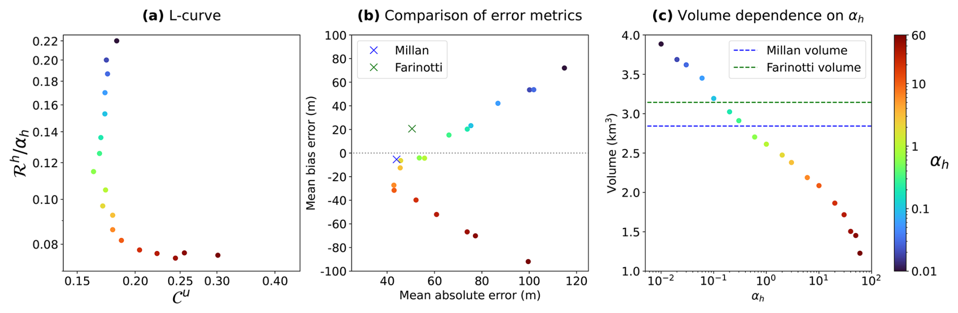
Figure 2 In each figure, each coloured point represents a unique value of α_h and its resulting thickness field. (a) L-curve relationship between 𝒞^u and ℛ^h. (b) Relationship between MAE and MBE. (c) Relationship between α_h and total volume.

During this experiment, we also measured the MAE and MBE between our final thickness field and the observed thicknesses. We found that the lowest MAE values (between 42–46 m) were achieved for ${\mathit{\alpha }}_h=\mathrm{2},\mathrm{3},\mathrm{6},\mathrm{10}$ (Fig. 2b), including values which were, incidentally, also found in the corner of the L-curve. The MBE values closest to zero (between −4 and −7 m) are achieved for ${\mathit{\alpha }}_h=\mathrm{0.6},\mathrm{1},\mathrm{2}$; however, the resulting thickness fields are visibly under-regularized compared to those achieved for higher values of α_h (e.g. Fig. C1b). Additionally, the thickness fields for ${\mathit{\alpha }}_h=\mathrm{0.6},\mathrm{1}$ show poorer accuracy in terms of MAE than the thickness fields for ${\mathit{\alpha }}_h=\mathrm{6},\mathrm{10}$. Figure 2b also demonstrates clearly that MAE and MBE need not be minimized simultaneously: the value of α_h producing the lowest MAE is not the same as the α_h with the lowest MBE.

Additionally worth noting is that the value of α_h appears to have a direct effect on the volume of the modelled glacier, with lower α_h corresponding to a higher final volume (Figs. 2c and C1), possible reasons for which are discussed in Sect. 4.1.

Based on the results found here, we acknowledge that there is no single optimal value of α_h. As the L-curve is a heuristic method, the choice of the “best” α_h among 2,3,6,10 is subjective. Note, however, that among these values, as α_h increases, the regularization cost decreases, but the magnitude of the MBE increases, and the velocity cost also increases slightly. We use the value α_h=6 in all of the following experiments, as it provides a good compromise between a well-regularized thickness field and a low MAE with observed thicknesses.

3.2 Cross-validation of thickness constraints

Figure 3a–d show the profiles chosen for each experiment described in Sect. 2.3.3. Figure 3e–h show the MAE against σ_h, for each of the four cross-validation experiments. In all four experiments, the error on the calibration set decreases as the strength of thickness constraint is increased (by decreasing σ_h). For all four experiments, the MAE on the calibration set drops below 10 m for any σ_h≤300, and is very small for any σ_h≤100. On the other hand, there does not appear to be a clear relationship between the value of σ_h and the validation set error, which remains between 32–45 m for all four experiments and all values of σ_h.

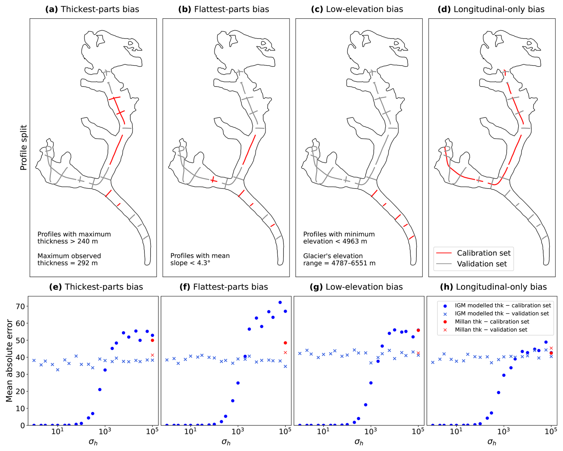
Figure 3 (a–d) Partitions of thickness observations on Bhote Kosi into calibration and validation sets, with red and grey lines representing profiles in the calibration set and validation set respectively. (e–h)  Mean absolute error of modelled vs observed thickness against σ_h for the above choice of calibration set. Blue markers denote the MAE in IGM thickness estimates at locations in the calibration and validation set. Red markers denote the MAE in the Millan thickness estimate at locations in the calibration and validation set. Circles and crosses denote the MAE on the calibration and validation set respectively.

Figure 4 shows the resulting thickness maps when constraining to no profiles (i.e. the velocity-only result), all available profiles, low-elevation profiles only and longitudinal profiles only.

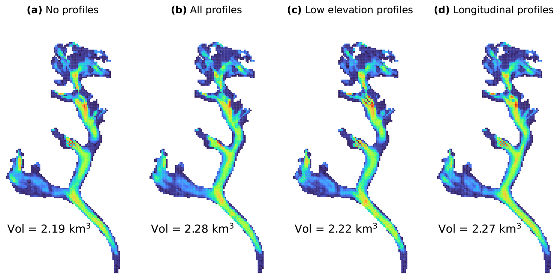
Figure 4 Thickness maps produced by IGM, obtained by constraining to (a) no thickness profiles, (b) all thickness profiles, (c) the low-elevation profiles highlighted in Fig. 3c, (d) the longitudinal profiles highlighted in Fig. 3d. In all cases the regularization parameter was α_h=6 and the thickness confidence parameter was σ_h=300. The colour scale for all panels is identical to that of Fig. 6a and b.

3.3 Sensitivity of inversion to Arrhenius parameter

The results of the experiment described in Sect. 2.3.4 are presented in Fig. 5. In Fig. 5a, we find that the lowest surface velocity cost is found for A=52 ${\mathrm{MPa}}^{-\mathrm{3}}{\mathrm{yr}}^{-\mathrm{1}}$, but that there is only a modest reduction of around 4.5 % in surface velocity cost against the result for A=78 ${\mathrm{MPa}}^{-\mathrm{3}}{\mathrm{yr}}^{-\mathrm{1}}$. Figure 5b shows that the lowest mean absolute error is achieved for A=52 ${\mathrm{MPa}}^{-\mathrm{3}}{\mathrm{yr}}^{-\mathrm{1}}$, but that the mean absolute errors for the results for A between 39–91 ${\mathrm{MPa}}^{-\mathrm{3}}{\mathrm{yr}}^{-\mathrm{1}}$ are all very close, lying between 39–42 m.

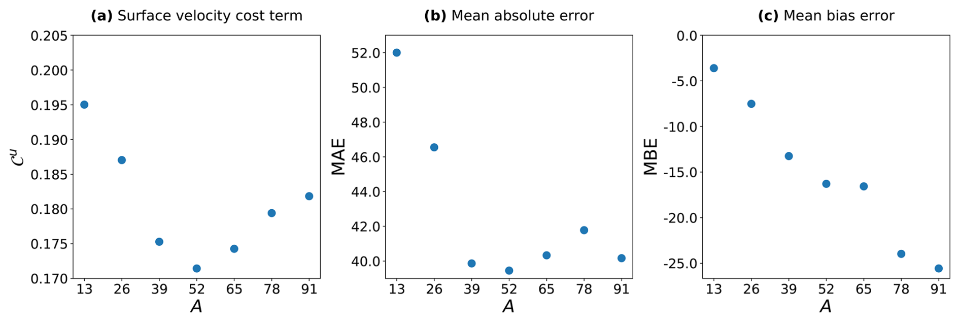
Figure 5 (a) Surface velocity cost term 𝒞^u (Eq. 3) against Arrhenius parameter A, (b) MAE against A, and (c) MBE against A.

In Fig. 5c, we see that the mean bias errors are negative for any A value. This is, however, consistent with our results from Fig. 2b showing that the mean bias error is negative for α_h=6. In general, increasing α_h has the effect of lowering the volume, whereas decreasing A corresponds to colder, stiffer ice, resulting in a higher volume (since a higher thickness is required to “explain” the same velocity). Low A values in this experiment are likely counteracting the choice of α_h which already resulted in a negative MBE (indicative of an underestimation of the glacier volume). The mean bias error closest to zero is achieved for A=13 ${\mathrm{MPa}}^{-\mathrm{3}}{\mathrm{yr}}^{-\mathrm{1}}$, but since this value also produces a very high mean absolute error, there is insufficient evidence to recommend this value.

4 Discussion

4.1 Effect of regularization parameter

We initially endeavoured to produce the “best possible” thickness field with velocity data only, by making a careful choice of the regularization parameter α_h, guided by the L-curve analysis in Sect. 3.1.

It is clear from our results that the choice of regularization parameter α_h has a strong effect on the final volume of the modelled glacier (Figs. 2c and C1). To understand why this is the case, observe that the regularization term (Eq. 5) is non-negative, and reaches zero if and only if ∇b=0 everywhere in Ω, i.e. when the bedrock elevation b is constant. Although the value of b does not change outside the glacier mask ℳ, flattening the bedrock inside ℳ and attempting to match the bedrock elevation at the boundary of ℳ will still reduce the regularization cost. In addition, the penalty term (Eq. 6) enforces zero thickness outside ℳ. These two effects together encourage low ice thickness h. This thinning effect is stronger when the regularization term ℛ^h is larger in comparison to the other terms in Eq. (2), i.e. when α_h is larger. Hence, increasing the value of α_h results in a decrease in modelled volume. Although this effect is somewhat undesirable, inclusion of a regularization term is nonetheless necessary to avoid non-physical small-scale spatial variations in the thickness field (as seen in e.g. Fig. C1a and b).

In future investigations it may be possible to avoid this undesirable effect through a reformulation of the regularization cost function. A potential strategy is to ignore gradients in the direction normal to the glacier boundary, within cells at the boundary. However, implementing such an approach is beyond the scope of our study.

4.2 Artefacts in thickness field

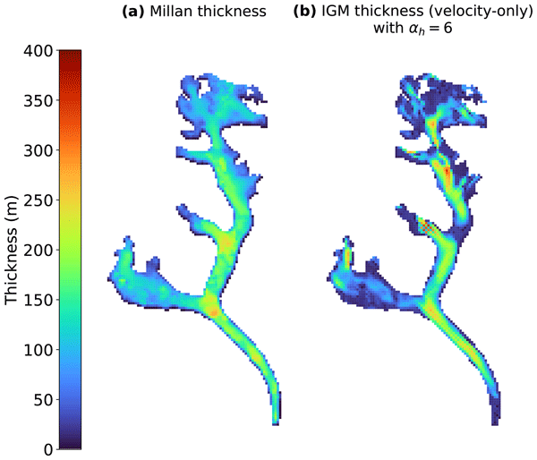
We observe in Fig. 6b that in the IGM estimate, there is an area of very low thickness present about halfway up the north tributary of the glacier, coinciding with a location where measured velocities are low (Fig. 7a). Small ice velocities are known to have high relative errors due to limitations associated with feature tracking methods (Dehecq et al., 2019). Since the ice is observed as almost stationary, there is insufficient information to infer the ice thickness from the surface velocity at this location. A similar issue may also be present at the area near the glacier terminus, as we also observe low velocity and low modelled thickness there. Despite using the same surface velocities from which the Millan estimate was derived, these low-thickness features were not present in the Millan estimate (Fig. 6a). This phenomenon was also observed on preliminary inversions of Ngozumpa and Lumsamba glaciers (not shown); however, although those glaciers are well-surveyed, we do not have sufficient thickness measurements for validation at the affected locations.

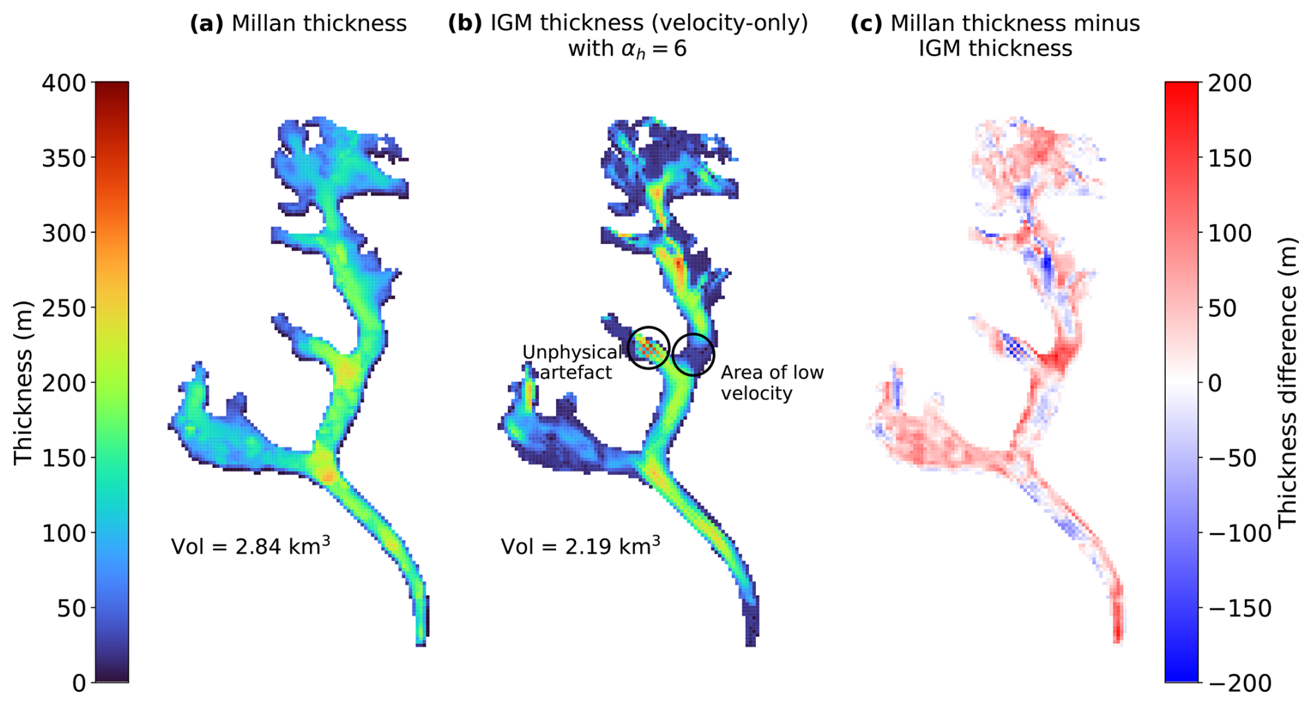
Figure 6 (a) The Millan thickness estimate of Bhote Kosi glacier, (b) the IGM velocity-only thickness estimate with the thickness regularization parameter set to α_h=6, and (c) the difference between the two.

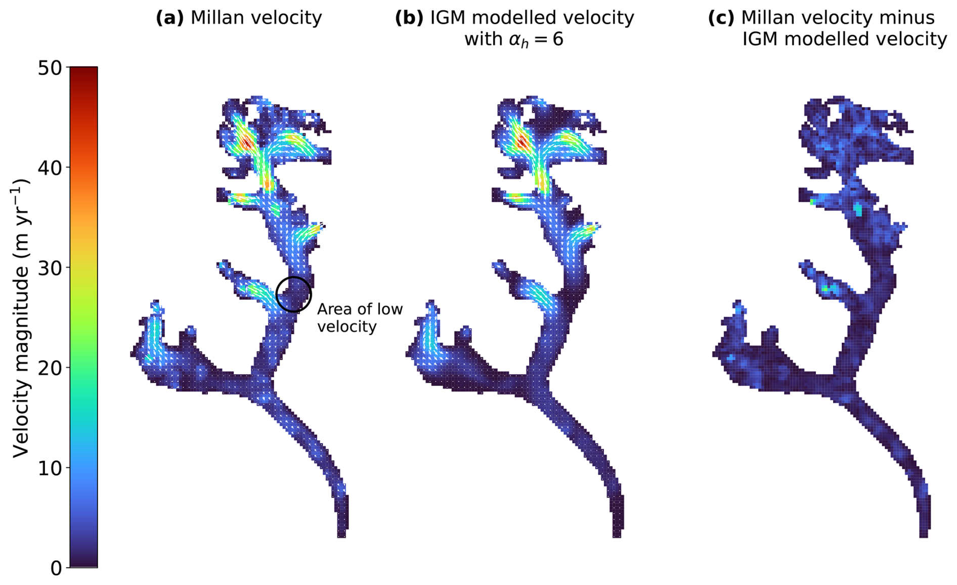
Figure 7 (a) The Millan velocity field of Bhote Kosi glacier, (b) the IGM modelled velocity field with the thickness regularization parameter set to α_h=6, and (c) the magnitude of the difference between the two.

Another non-physical artefact visible in the resulting thickness field (Fig. 6b) is checkerboarding, which is particularly apparent in the tributary halfway up the north tributary of the glacier, immediately to the west of the “low-velocity” area. This artefact is likely the result of the approximation of spatial gradients with simple finite differences in the cost function, which can produce undesirable modes. Further work is required to address this issue within IGM. In the present case, we found that this artefact was triggered most severely in a region showing discontinuity in the input velocity field, and vanishes when using smoothed data (Appendix D).

4.3 Error in velocity-only estimate and comparison with Millan estimate

In our velocity-only inversion, we succeeded in making a reconstruction of the thickness field with errors comparable to the Millan estimate by using surface velocity data only. The observed thickness data (which was not available at the time the Millan estimate was published) was valuable in this experiment to validate the results, as otherwise, we would have had no way of validating the accuracy of our results, or indeed the Millan estimate. While it is not appropriate to consider the difference between our velocity-only thickness estimate and that of Millan et al. (2022) as an “error”, as neither study represents the ground truth, it is of interest to compare the two results, as both attempt to estimate glacier thickness based on the same surface velocity data, without using observed thickness.

Interestingly, in Fig. 8, we observe that IGM produces a more accurate representation of the thickness of the west tributary as compared to the Millan estimate. Measurements show that the west tributary is significantly thinner than the main trunk and north tributary, a detail that is reproduced by IGM even when it is given no direct information about the thickness in this location. Furthermore, Millan generally overestimates thickness in the west tributary, while underestimating thickness in the rest of the glacier. Improvements by IGM over the Millan study may be due in part to higher-order physics, since IGM is based on the Blatter–Pattyn model, while Millan used the SIA, which excludes stress components which are non-negligible in mountain glaciers.

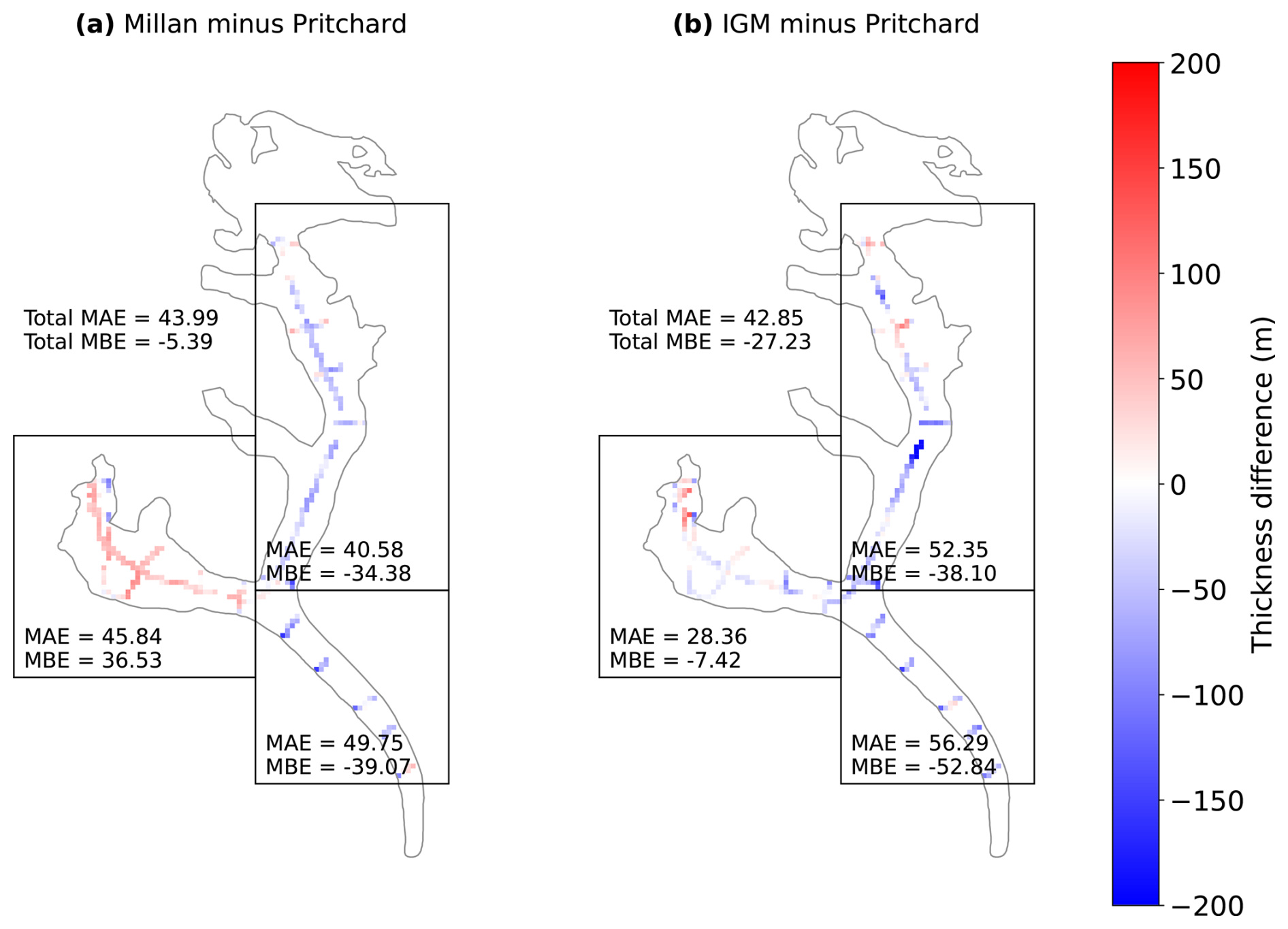
Figure 8 (a) The difference between the Millan thickness estimate and the rasterized thickness observations from Pritchard et al. (2026), and (b) the same for the IGM velocity-only (α_h=6) thickness estimate. Bhote Kosi glacier is split into three regions and the MAE and MBE of each model is shown for each region.

The IGM-inverted thickness exhibits poorer accuracy in the north tributary as compared to Millan, an error which can be attributed in part to the underestimation of the thickness at the low-velocity area discussed in Sect. 4.2. We observe also that both Millan and IGM underestimate the thickness of the main trunk of Bhote Kosi (Fig. 8).

Pritchard et al. (2026) compared their observed thicknesses with the Millan and consensus estimates, finding that both estimates are biased, with errors of over 100 m in places. In our velocity-only inversions, no value of α_h succeeded in bringing the MAE below 42 m (Fig. 2b), indicating that significant bias is also present in our estimated thickness field. Relative errors (not shown) are over 50 % in several places, and over 100 % in a handful of locations. Such biases undermine the efficacy of these thickness products when predicting the evolution of a glacier over time. In the case of IGM, the systematic underestimation of thickness may result from the implementation of the regularization term (as discussed in Sect. 4.1). Additionally, although IGM is based on the Blatter–Pattyn model, which contains higher-order stress terms that are missing from the SIA as used by Millan, it is still not a full-Stokes model. The use of a neural network as an emulator for the Blatter–Pattyn model, rather than a true solver, may also compromise IGM's accuracy, although high-fidelity results have been achieved previously (Jouvet and Cordonnier, 2023).

4.4 Physically consistent ice thickness

Inter-comparison exercises (Farinotti et al., 2017, 2021) focus on assessing the quality of thickness estimates by error with unseen measured thickness, but one can also consider a high-quality thickness estimate as one which yields an ice velocity field which is consistent with both data and physics. Although our velocity-only IGM thickness estimate is of comparable accuracy to Millan's thickness estimate when considering MAE or MBE across all measured thicknesses over the entire glacier, it does have the additional benefit of higher-order physical consistency between modelled thickness and satellite-observed velocity data. IGM achieves this by enforcing low misfit between modelled and observed surface velocity (Eq. 3) during the thickness optimization.

4.5 Cross-validation and interpolative power of thickness constraints

In Fig. 3, we observe that increasing the strength of the thickness misfit term (Eq. 4) effectively reduces the MAE on the calibration set, but does not reduce the MAE on the validation set. The MAE on the validation set remains between 32–45 m for all four partitions of the data and all values of σ_h, showing at best a modest reduction from the MAE of more than 42 m achieved when omitting thickness profiles from the inversion (Sect. 3.1). This indicates that the thickness observations have limited interpolative power in this model setup, i.e. constraining to thickness observations has only a weak effect on the accuracy of the modelled thickness at unconstrained locations. This is further confirmed by Fig. 4, which shows the resulting thickness map when taking σ_h=300 and constraining to different subsets of the available thickness profiles. We see that the thickness distribution constrained to all profiles (Fig. 4b) appears largely the same as that obtained without thickness constraints (Fig. 4a), with only local-scale changes visible in the resulting thickness map, and a small increase in total volume. We observe also that between the thickness maps obtained by constraining to low-elevation profiles (Fig. 4c) and longitudinal profiles only (Fig. 4d), the calibration sets in these two cases have no profiles in common and no intersection between profiles in the two sets. Both thickness fields look very similar to the velocity-only thickness field at locations without observations.

While this result indicates that overfitting to observed thicknesses is not an issue, it also indicates that constraining to thickness observations has little effect on the thickness at unconstrained locations with this modelling approach. A potential reason for the low interpolative power of thickness observations is the limited spatial influence of stress perturbations according to the Blatter–Pattyn stress balance. Changes in speed and driving stress are felt over the membrane length scale (Robinson et al., 2022), typically on the order of a few ice thicknesses. In the present context, consider a location where there are no thickness constraints. If a thickness constraint is introduced close by, this will influence velocities at the location, and the optimization therefore will need to adjust thickness at the location in order to reduce the misfit with observed surface velocities. If the introduced thickness constraints are sufficiently far away, the influence on velocity is minimal, and therefore so is the adjustment. With strong enough regularization, there could be a smoothing length scale that is larger than the membrane length scale, leading to non-physical interpolation of thickness constraints.

The disappearance of the erroneous low-thickness zone in the north tributary when adding thickness constraints (compare Fig. 4a and b) highlights the importance of constraining to thickness profiles where available, as in this case their inclusion was able to correct for a lack of information from the surface velocity data.

We point out that some methods to estimate thickness involve “flux conservation” (Farinotti et al., 2009) or “mass conservation” (Morlighem et al., 2011, 2013), in which the depth-integrated glacial mass balance equation essentially propagates information down-glacier or away from thickness profiles, explicitly carrying information to non-measured areas of the glacier. These methods, however, either require accurate surface mass balance information, which is difficult to obtain in our region, or depend on surface mass balance parametrizations at a regional level. Importantly, our approach is distinct from these continuity-based methods in that it provides a thickness that is dynamically consistent with a higher-order stress balance, making it more suitable for subsequent model investigations.

4.6 Arrhenius parameter

IGM's default value for A is 78 ${\mathrm{MPa}}^{-\mathrm{3}}{\mathrm{yr}}^{-\mathrm{1}}$, which heuristically corresponds to temperate glaciers around 0 °C (Cuffey and Paterson, 2010, Table 3.4), and may not be optimal for glaciers in HMA. On the other hand, the value used by Millan for glaciers in the Everest area was 13 ${\mathrm{MPa}}^{-\mathrm{3}}{\mathrm{yr}}^{-\mathrm{1}}$, which was based on a very small number of thickness observations for glaciers elsewhere in HMA. Their value approximately corresponds to between −5 and −10 °C (Cuffey and Paterson, 2010, Table 3.4), colder than measured englacial temperatures on nearby Khumbu glacier (Miles et al., 2018). Indeed, the use of different values of A may partially explain why Millan's modelled volume is slightly higher than ours (Fig. 6): when directly estimating thickness via the SIA (Millan et al., 2022, Eq. 2), there is an inverse relationship between A and ice thickness.

We acknowledge that using a different Arrhenius value for our previous experiments may change our results slightly (Fig. 5), but we did not identify an ideal value. If we were to switch to a different (spatially constant) value of A, the aspect of our result that would be most affected would be the glacier volume (Fig. 5c). However, changing A would be unlikely to affect our earlier conclusions: that the regularization parameter α_h affects the volume and can be optimized with L-curve analysis, and that tuning the thickness confidence parameter σ_h reduces the error at locations with thickness observations seen by the model, but seems to have little effect on unseen thickness observation locations. Future work could consider spatially varying A, a scenario which is more realistic since englacial temperatures (and therefore A) may vary throughout a glacier.

4.7 Contemporaneity of input data

As mentioned in Sect. 2.2, the acquisition dates of the DEM are from 2010–2015, while the velocity observations are from 2017–2018, and the thickness observations are from 2019. We consider the nominal date of our thickness inversions to follow that of the velocities, which are relatively close in time to thickness observations. However, they are separated from the surface elevations used for the DEM by 3–8 years. This is still a short time relative to glacial evolution time scales, though it potentially introduces uncertainties in our thickness estimates.

Recent surface elevation change rates on Bhote Khosi have been observed at approximately −2 m yr⁻¹ (Hugonnet et al., 2021), which implies the DEM surface is approximately 6–16 m higher than at the time of velocity acquisition. As the relationship between velocity, surface, and recovered thickness is non-local and complex, it is difficult to quantify the relationship between this surface bias and any resulting bias in estimated thickness. Regardless, the bias in surface elevation is relatively small, and in particular, smaller than the errors in estimated thickness in comparison with the thickness observations (Fig. 8b). Thus, we do not expect non-contemporaneity of our inputs to be a major source of uncertainty in our study.

On the other hand, even small errors arising from non-contemporaneity can lead to dynamical imbalance which causes spurious behaviour in model projections, as seen in similar settings in ice-sheet models (Schmitt et al., 2026). Therefore, it is important to ensure different data sources are as close in time as possible.

4.8 Applicability to other glaciers

Our results demonstrate that a lack of thickness observations need not be a barrier to producing a reasonable thickness estimate, as we were able to produce results with estimated accuracy comparable to the leading thickness estimates by constraining to surface velocity data alone, by making an informed choice for the regularization parameter α_h. Although our results showed that significant bias was present in non-thickness-constrained results, and that thickness constraints introduced only limited changes to the thickness at unconstrained locations, results on other glaciers may vary.

For a glacier with no thickness observations (which is the case for most glaciers), there is no way to perform a validation test against the true thickness, and therefore it would not be possible to create a plot equivalent to Fig. 2b. Regardless, it would still be possible to create an L-curve plot similar to Fig. 2a, and, assuming the desired L-shape is present, choose a value in the corner of the L (indeed, for this example we could have chosen the value α_h=6 based on this alone). In our example, the α_h values in the corner of the L-curve also gave a low MAE. It would also be possible to compare the total volume with the consensus and Millan total volumes, as in Fig. 2c: while neither of these studies represent the ground truth, this comparison serves as a consistency check to flag up any thickness fields whose volume deviates implausibly from other estimates.

Preliminary inversions were performed on the other 12 glaciers (as outlined in RGI v6.0) with thickness observations from Pritchard et al. (2026). The parameters found to be optimal for Bhote Kosi were used (α_h=6, σ_h=300), with results (not shown) varying in quality. Very low modelled volume was observed for multiple glaciers, particularly smaller glaciers where a resolution of 100 m may not be fine enough to resolve physical details. This demonstrates that the parameters, particularly α_h, may be somewhat glacier-dependent. We note that the term 𝒞^u (Eq. 3) involves a mean over the glacier mask ℳ, but ℛ^h (Eq. 5) involves a mean over the rectangular domain Ω. When switching to a different glacier, the ratio between the areas of ℳ and Ω is likely to be slightly different. This is one factor that may affect the regularization parameter required. In order to produce accurate thickness maps for other glaciers, a full L-curve analysis per glacier would likely be beneficial. A finer spatial resolution may also be required for smaller glaciers.

4.9 Recommendations for observation locations

Farinotti et al. (2021) found that it is advisable not to have all thickness observations concentrated at the lowest elevations of the glacier, and that covering the thickest parts (which often coincide with the flattest parts) is the most effective way to ensure accurate volume estimation.

Our investigation demonstrated that there is a lack of “signal” from low-velocity locations, which often leads to erroneous low modelled thickness, as thin ice can also yield a similar near-stagnant ice flow. This effect can be corrected by the inclusion of a thickness profile for calibration. We therefore propose, in addition to the above considerations from Farinotti et al. (2021), that fieldworkers should aim to measure the thickness at such low-velocity areas, because this may the best way to ensure accuracy at those locations when estimating thickness.

Conversely, thickness observations are also valuable in fast-flowing locations, since this is where velocity inversions are most effective. In such locations, thickness observations can aid in model-parameter optimization, i.e. the choices of α_h and A in our setup. Furthermore, the membrane length scale is longer where there is faster ice flow, thereby increasing the interpolative power of thickness observations.

Following the discussion in Sect. 4.5, we reiterate that the inclusion of thickness constraints does not guarantee improved estimates of thickness at distant locations. Therefore, in our setup, the calibration of ice thickness at locations with no nearby measurements relies heavily on making optimal choices for the model parameters α_h and A.

5 Conclusions and further work

In this study, we used IGM's higher-order (as compared to previous thickness estimation methods) inversion capabilities to produce glacier ice thickness estimates that are physically consistent with surface velocity data, exploring methods for choosing inversion parameters. By leveraging a novel dataset of glacier thickness observations, we were able to compare results obtained by additionally constraining to observed thicknesses.

When constraining to surface velocities only, we found that the accuracy of the resulting thickness field depends strongly on the choice of the thickness regularization parameter, with a suboptimal choice resulting in poor agreement with true thickness, and a potentially inaccurate total volume. Furthermore, the thickness regularization parameters chosen via an L-curve approach coincided with those resulting in the lowest achieved MAE with observed thicknesses, indicating that in the absence of thickness observations (the situation for most glaciers), picking the right regularization parameter is an effective way to ensure accuracy. However, the lowest achieved mean absolute error was above 40 m, which is relatively large for this glacier: its maximum observed thickness is 292 m. The high errors present in all three non-thickness-constrained estimates (consensus, Millan, and non-thickness-constrained IGM) indicate that there is still significant bias present in all three approaches.

Our thickness-constrained inversion results demonstrate that while observational thickness data were of some value for constraining our thickness estimate of Bhote Kosi glacier, they had only a weak influence on the final thickness field, and their interpolative power was limited. However, the thickness observations were highly valuable as validation data, whether performing velocity-only or thickness-constrained inversions. Since the HMA region still has poor data coverage, further effort is required to gather more thickness observations. Contemporaneity between input data sets is especially important for dynamical consistency in modelling glaciers that are out of steady state. Since we observed that the inversion method struggles to estimate thickness in areas with a low measured surface velocity, we propose that fieldworkers should aim to measure thickness at such locations where possible, in addition to fast-flowing areas where thickness observations can aid in selecting model parameters.

Further work is required to apply our method to other glaciers. As preliminary results on other glaciers in the region were of varying quality, the optimal choice of regularization parameter may be glacier-dependent, and it may be necessary to perform L-curve analysis for individual glaciers. Future work could also consider a more robust method for determining the Arrhenius parameter, perhaps allowing for spatial variability.

Appendix A: Convergence of inversion

Figures A1a and A2a show the convergence of the cost function (Eq. 2) over 1000 iterations of the inversion algorithm. The velocity misfit term 𝒞^u and the regularization term ℛ^h both appear to converge to a constant value after around 100–200 iterations, with only small fluctuations thereafter. In the case of the thickness-constrained inversion (Fig. A2a), the thickness misfit term 𝒞^h behaves similarly, converging fairly soon after initialization and exhibiting only small fluctuations thereafter. On the other hand, the penalty term 𝒫^h behaves as if it is either “on” (a very high number) or “off” (zero or very close, meaning there are virtually no negative thicknesses present and no positive thicknesses present outside the mask ℳ) at each iteration. Its presence manifests as intermittent “spikes” in the cost over iterations, indicating that the inversion algorithm quickly corrects for negative thicknesses and non-zero thicknesses outside ℳ. The frequency of the spikes tends to decrease with more iterations.

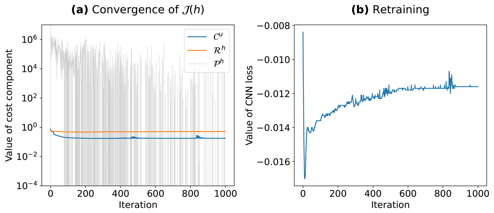
Figure A1 Progression of (a) the value of the cost function (Eq. 2) and (b) the value of the neural network emulator loss, over iterations of the inversion algorithm, for the velocity-only inversion with α_h=6.

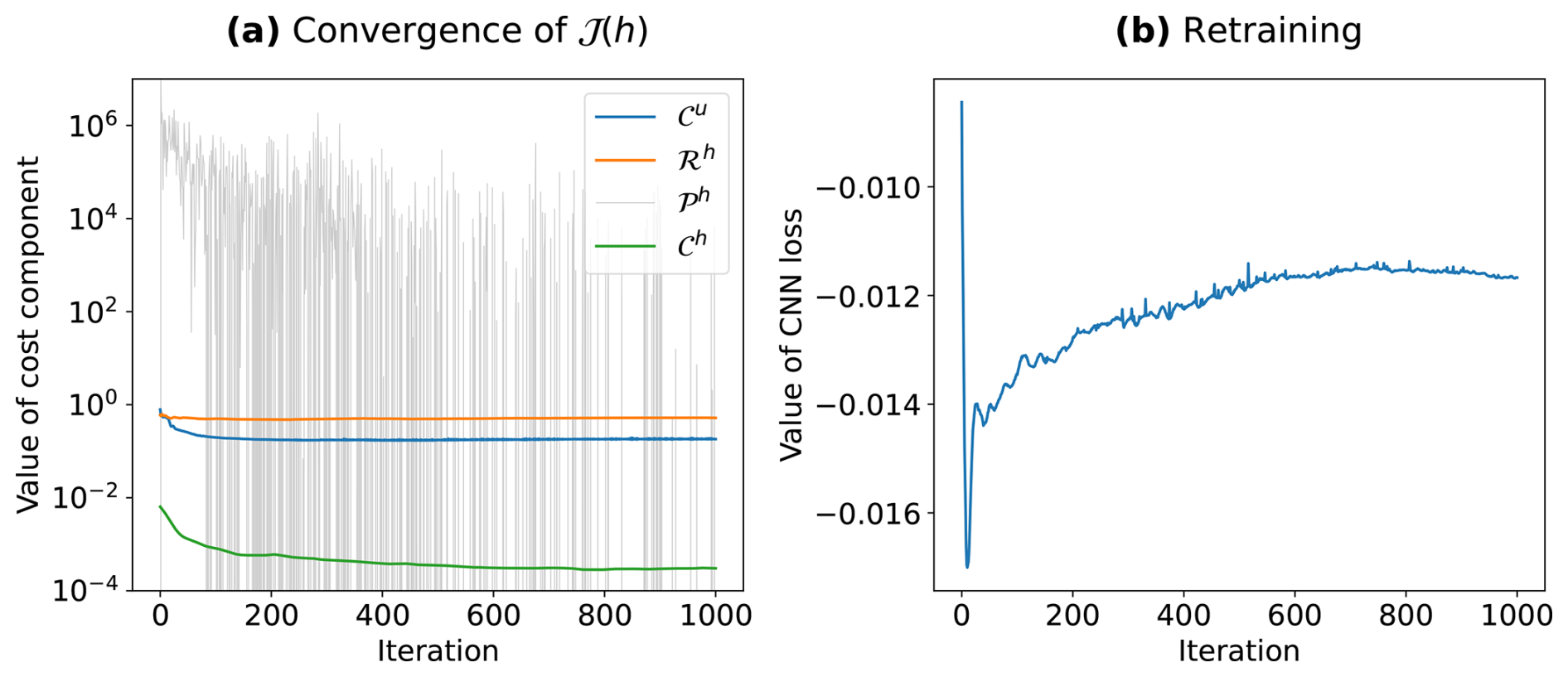
Figure A2 Progression of (a) the value of the cost function (Eq. 2) and (b) the value of the neural network emulator loss, over iterations of the inversion algorithm, for the thickness-constrained inversion with α_h=6, σ_h=300, and the calibration set consisting of low-elevation profiles only.

Figures A1b and A2b show examples of how the neural network loss (the energy functional associated with the Blatter–Pattyn equations) evolves over the iterations of the inversion algorithm. In both cases, the loss converges towards a constant value after around 600 iterations.

Appendix B: Presence of thickness observations outside glacier outlines

Figure B1 shows an example location where there are thickness observations outside the glacier outline, and where the outline does not align perfectly with the outline of the glacier in recent satellite imagery.

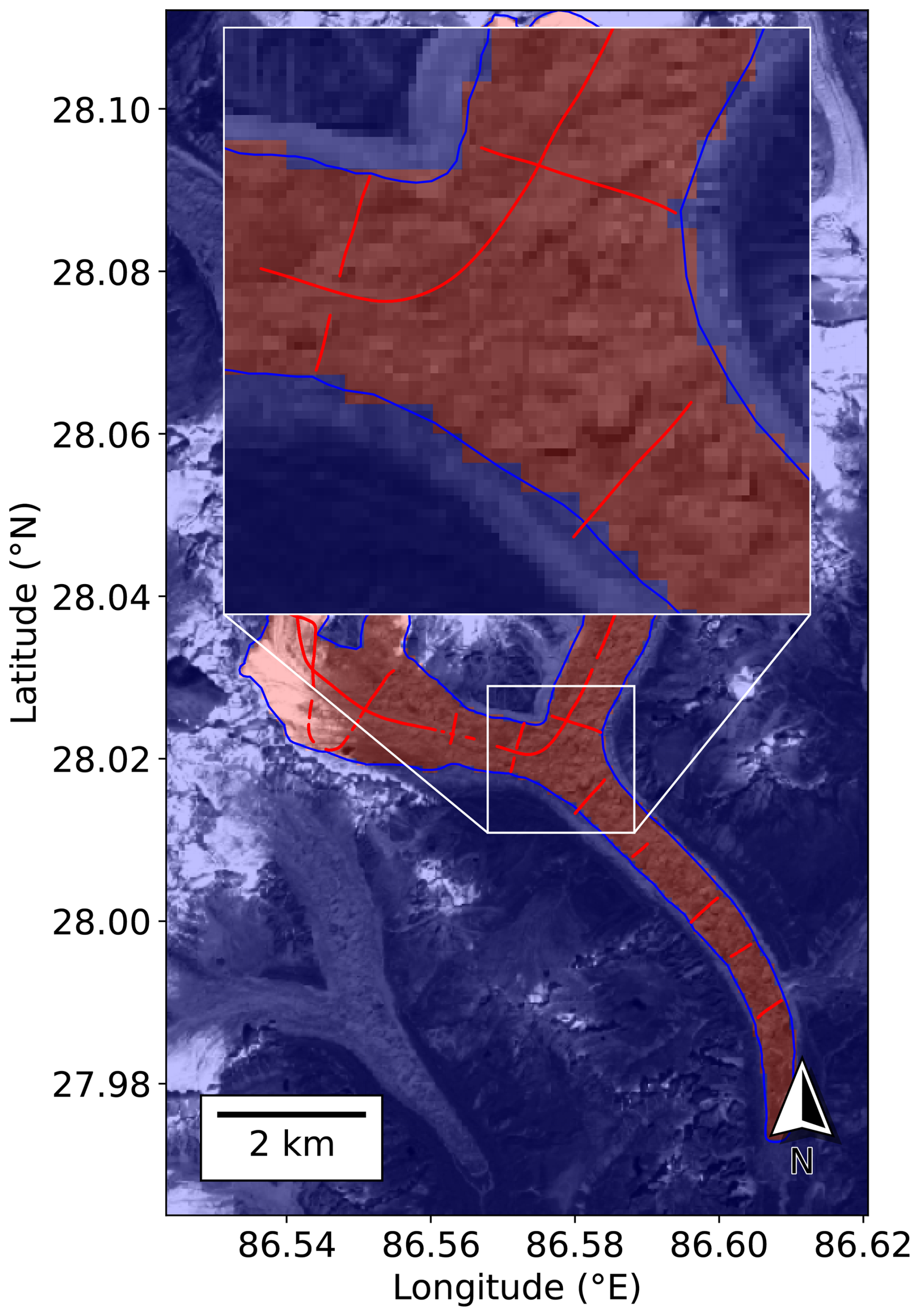
Figure B1 RGI v6.0 outline of Bhote Kosi glacier in blue. Locations of Pritchard et al. (2026) thickness observations in red. Red/blue overlay denotes the area inside/outside the rasterized glacier mask. Background image is a Sentinel-2 scene (band 04) from 15 October 2019 (contains modified Copernicus Sentinel data [2019] processed by Sentinel Hub).

Appendix C: Effect of regularization weight α_h on smoothness and total volume of solution

Figure C1 shows four thickness fields obtained by the velocity-only inversion, with different values of the regularization parameter α_h.

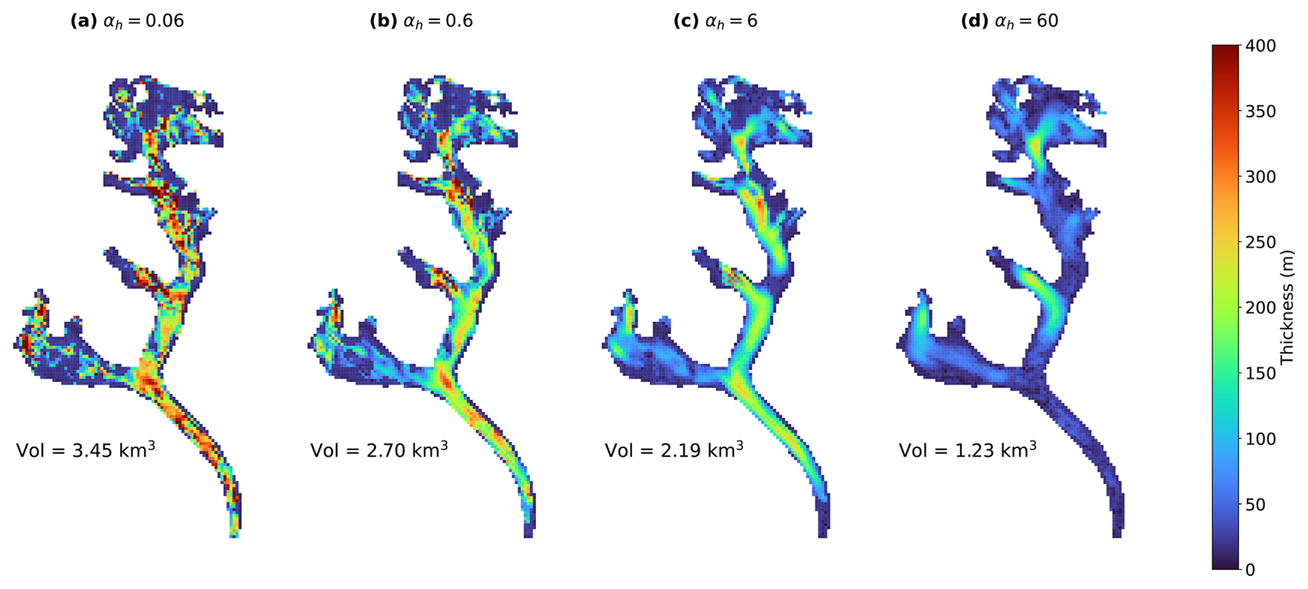
Figure C1 Thickness maps of Bhote Kosi glacier for four different choices of the thickness regularization parameter α_h: (a) α_h=0.06, (b) α_h=0.6, (c) α_h=6, (d) α_h=60.

Appendix D: Exaggerated checkerboarding artefact

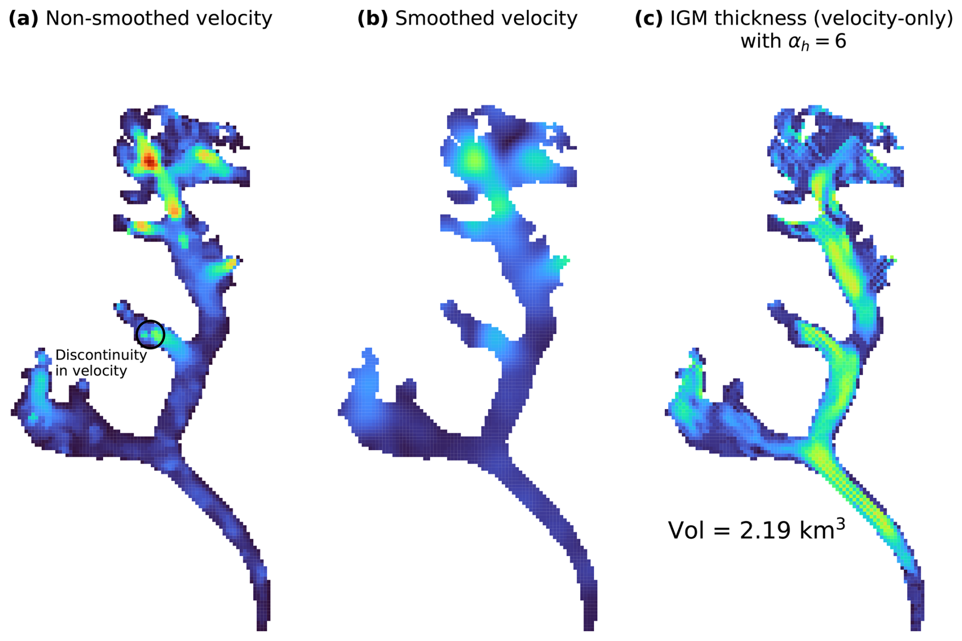
Figure D1 (a) Identical data and colour scale to Fig. 7a but only velocity magnitude is shown, (b) smoothed version of the input velocity field shown in Fig. 7a with only velocity magnitude shown, and (c) the resulting thickness field as estimated by IGM under a velocity-only inversion scheme with regularization parameter α_h=6 and attempting to match the velocity data shown in (b), with the same colour scale as Fig. 6a and b.

Figure 6b shows a non-physical checkerboard artefact in the tributary halfway up the north tributary of the glacier. A closer look at the input observed velocity field (Figs. 7a and D1a) shows a slight discontinuity in the velocity around that location: from west to east, the speed dips from 15–20 m yr⁻¹ to around 5–10 m yr⁻¹, and increases again to around 15–25 m yr⁻¹, and the direction of the velocity also reverses.

An experiment was performed whereby the input velocity field was smoothed using a Gaussian filter with standard deviation 3 (Fig. D1b). We emphasize that the purpose of this experiment was solely to test the hypothesis that the jump in velocity at the problem location could be triggering non-physical artefacts in the modelled thickness field.

The resulting thickness field as estimated by IGM under a velocity-only inversion scheme is presented in Fig. D1c. The checkerboard at that location is now less pronounced, suggesting that the jump in velocity may have triggered the artefact.