SeidarT: an open-source full-waveform seismic and electromagnetic wave propagation modeling toolbox demonstrated in snow and ice

We present SeidarT, an open-source, community-driven software package for full-waveform finite-difference time-domain (FDTD) modeling of elastic and electromagnetic wave propagation in heterogeneous, anisotropic, and attenuating media. SeidarT natively incorporates full-tensor anisotropy (all 21 stiffness coefficients), frequency-independent attenuation through a generalized Q formulation, and unified treatment of both seismic and electromagnetic wave physics on a simple Cartesian grid. The software prioritizes accessibility and extensibility by combining the computational efficiency of Fortran with the user-friendly scripting capabilities of Python. Model construction leverages an intuitive image-based geometry workflow and JSON project files, eliminating the need for complex mesh generation while allowing flexible specification of arbitrary stiffness or permittivity tensors, material distributions, and boundary conditions. We implement the Convolutional Perfectly Matched Layer (CPML) with explicit tuning strategies adapted for anisotropic media, and provide automatic stability checking via the Courant-Friedrichs-Lévy and wavenumber-bandlimit criteria. The software is validated against analytical solutions for elastic wave propagation and empirically constrained through comparison with ground-penetrating radar and seismic field observations in snow and ice. We document the physical property parameterizations for ice and snow as functions of temperature, pressure, and liquid water content, and provide multiple material homogenization schemes (Hill average, Gassmann substitution, Self-Consistent Approximation) to accommodate variable porosity and fluid saturation regimes. SeidarT is designed to lower economic and technical barriers for scientists, engineers, and students integrating sophisticated wave-physics simulations into workflows spanning cryospheric research, environmental monitoring, subsurface characterization, and civil infrastructure assessment. The open-source development model on GitHub and PyPI encourages community contributions and iterative improvements, positioning SeidarT as a versatile platform for advancing both fundamental understanding and applied geophysical imaging.

1 Introduction

Wave propagation modeling plays a central role across a wide range of disciplines – from exploration seismology using elastic (Hu et al., 2023; Lyu et al., 2025) and environmental monitoring (Graves and Day, 2003) to civil infrastructure assessment (Komatitsch and Vilotte, 1998; Ali et al., 2023) and planetary science (Bozdağ et al., 2017) – by providing detailed insights into subsurface and structural properties that are otherwise inaccessible. Whether probing for groundwater reservoirs (Gueting et al., 2017), characterizing fracture networks in geothermal fields (Jiang et al., 2023), imaging buried archaeological sites (Miller et al., 2018), or evaluating the integrity of concrete bridges (Hugenschmidt and Mastrangelo, 2006), elastic and electromagnetic waves offer non-invasive means of imaging and characterizing the subsurface. Numerical experiments are particularly valuable when direct measurements are impractical or hazardous, enabling parameter studies, sensitivity analyses, and synthetic data generation for developing advanced processing workflows, including machine-learning approaches in regions with sparse field observations (Wu et al., 2019; Witsil et al., 2022).

Numerical solvers for wave phenomena are ideal in situations where complex mathematics and modeling domains do not allow for analytical solutions, such as when heterogeneity, anisotropy, attenuation, or irregular boundaries make closed-form solutions intractable. Modeling approaches can be categorized using two different methods: (1) full waveform, which includes Finite Difference Time Domain (FDTD) (Levander, 1988; Virieux, 1984; Komatitsch and Martin, 2007), Finite Element Method (FEM) (Zienkiewicz et al., 1977; Mahmoudian and Margrave, 2003), pseudo-spectral (Klin et al., 2010), and spectral element methods (Komatitsch and Tromp, 1999), and (2) ray tracing methods (Julian and Gubbins, 1977; Um and Thurber, 1987). Although ray tracing methods are computationally less expensive yet effective in modeling travel time of specific modes, full waveform techniques provide the elastodynamic response, capturing the time variability of wave phenomena (Bai et al., 2013).

Implementing full-waveform solvers in heterogeneous, anisotropic media poses significant challenges: meshing complex geometries for spectral or finite‐element schemes can become unwieldy, while high‐order finite differences must carefully balance accuracy, stability, and computational cost. In snow and ice, for example, preferred crystal‐orientation fabrics, varying water content, and thermal gradients introduce full‐tensor anisotropy and frequency-dependent attenuation that significantly alter both seismic and electromagnetic responses (Bradford et al., 2009; Bælum and Benn, 2011; Riche et al., 2013; Montagnat et al., 2020). Similar complexities arise in subsurface petroleum systems (fractured carbonates, shales), geotechnical investigations (i.e. seismic site amplification, reinforced concrete GPR imaging), anthropological/archaeological surveys (preferential artifact orientations, heterogeneous burial stratigraphy, disturbed sediments) and even biomedical ultrasound (i.e. anisotropic soft tissues), motivating a need for versatile modeling frameworks that can flexibly accommodate a variety of physical parameters and boundary conditions.

In this work, we present SeidarT, an open-source FDTD code that natively incorporates full‐tensor anisotropy, frequency‐independent attenuation (via a generalized Q formulation) (Kjartansson, 1979), and both seismic and electromagnetic wave physics within a unified, computationally efficient environment. Its design emphasizes simplicity of implementation – avoiding complex mesh generation – while allowing users to specify arbitrary stiffness or permittivity tensors, material distributions, and boundary conditions by coupling an image-based geometry and JSON project workflow. The software package is validated against analytical solutions and snow/ice-focused field observations, and includes explicit treatment of the Convolutional Perfectly Matched Layer (CPML) tuning and stability in anisotropic media with a focus on cryospheric applications. As computing power becomes increasingly accessible, SeidarT is designed to lower economic and technical barriers by providing a ready-to-use, extensible framework that scientists and engineers can integrate into workflows ranging from cryospheric research and hydrocarbon exploration to civil–environmental engineering.

2 Software Description

2.1 Key Features and Architecture

SeidarT is designed to enhance usability and performance in geophysical modeling, particularly for wave propagation in snow and ice environments. One of its key features is that it is open-source and hosted on GitHub, accompanied by robust documentation to support users in its implementation and development. Its architecture is designed to be open and extensible, making it easy to integrate with additional Python packages or other scripting languages as needed. The design philosophy follows a modular and flexible approach to cater to a wide range of geophysical applications and user skill sets. The core of the software is built around the staggered grid finite difference time domain (FDTD) method, which provides robust and accurate solutions for 4th order seismic and 2nd-order electromagnetic wave propagation.

Model development in SeidarT leverages illustration software used to generate PDF and PNG files. There are open source tools such as GIMP and Inkscape, but the actual choice is the user's preference. This approach provides users with significant control over defining complex geometries, such as the varying sloped sidewalls and changes in ice facies found in glaciers. Programmatically defining such intricate geometries can be cumbersome and limiting, whereas using RGB values in raster based illustrations to identify different materials streamlines the process, allowing for more precise and versatile model creation.

Models are organized in a JSON (JavaScript Object Notation) file (Bray, 2017) where users can define domain parameters, source locations, and the properties associated with the materials present within the domain. The use of JSON provides a readable platform, and this approach streamlines the setup and management of simulations, making it straightforward to configure and run their models.

The software supports the calculation of bulk properties from Euler angle inputs for material fabrics, but material tensors can be manually input when available. Users can input text files from Electron Backscatter Diffraction (EBSD) directly into the program for material homogenization, employing three Euler angles for Bunge rotation (z–x–z) (Bunge, 2013) and fourth-order tensors. This allows for detailed incorporation of natural sample (i.e. ice core) observations, which can then be compared with Ground Penetrating Radar (GPR) and seismic observations, in order to provide correlation between observed and modeled data.

2.2 Workflow

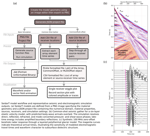
Building and creating a wave propagation model follows the simple image plus JSON workflow (Fig. 1). A rectilinear Cartesian grid with uniform spacing along each coordinate direction, represented by a PNG image, establishes the simulation domain, where each pixel corresponds to an FDTD node and each color is automatically assigned an integer ID. This ID serves as a relational value that is later referenced in the model configuration to link material properties and wave parameters to regions in the grid. With the PNG defined, the user creates a JSON project file specifying domain attributes (dimensions, resolution), material settings (e.g., stiffness or permittivity and conductivity tensors), and model parameters (seismic or electromagnetic mode). Tensors can be supplied explicitly or generated, and for 2.5D simulations the x–z plane properties are extruded in the y-direction with corresponding CPML settings.

Figure 1 The general workflow tree for creating a wave propagation model and survey simultations. All of the simulations are supersets of the basic simulation. The common shot gather can be built post run making it possible to build different array configurations without rerunning the model.

Only two files are strictly required to run a simulation: the JSON project file and the PNG image. At build time, the user specifies at least the number of time steps and source center frequency, and may optionally define initial conditions. SeidarT automatically checks that the grid spacing and velocity model satisfy the Courant–Friedrichs–Lewy (CFL) condition and chooses a stable time step (Courant et al., 1928). Default CPML parameters are also initiated using in ranges provided by (Roden and Gedney, 2000), but these values can be tuned individually to improve boundary performance. While running the simulation, outputs are written either as Fortran unformatted binary files (.dat) at each time step or chunked block outputs compressed using Zstandard formatting (Collet and Kucherawy, 2021). This increases storage requirements with the tradeoff of preserving the full wavefield, allowing post hoc construction of arbitrary receiver arrays and extraction of particle-velocity or electric-field time series at any node, including dense virtual-sensor networks.

SeidarT supports common-offset profiling by extending internal class variables to generate series of model runs. For common-offset surveys, a CSV file specifies paired source and receiver locations, with each row containing a source–receiver pair. Results from common shot gathers and common-offset surveys can be exported as pickle-formatted files and/or CSV files. Pickle files retain model parameters and metadata, time series, and derived products within a single object, while CSV output facilitates import into external signal-processing workflows. Receiver geometry for common-offset surveys is fixed for a given run, so changing array layout requires rerunning the survey, but the modular design makes it straightforward to set up, rerun, and analyze different acquisition scenarios.

3 Computational Framework

3.1 Governing Equations

Wave propagation refers to the manner in which elastic (seismic) or electromagnetic perturbations travel through often heterogeneous materials. Accurately capturing those waves – especially in anisotropic or attenuating media – requires a discretization strategy that resolves both fine‐scale interfaces and broad‐scale structures. While finite‐element (FEM) and spectral‐element (SEM) methods offer high accuracy per degree of freedom, they introduce substantial implementation complexity and often rely on external libraries. By contrast, a finite‐difference time‐domain (FDTD) approach, though computationally heavier, remains remarkably minimalist: it directly discretizes Maxwell's equations (for EM) or the elastodynamic equations (for seismic) on a simple Cartesian grid. This simplicity makes the codebase easier to inspect, modify, and extend.

The FDTD approach has undergone continuous refinement to handle increasingly complex media and boundary conditions. Maxwell's equations or the equations of motion can be discretized using a grid where the electric and magnetic field (or stress and velocity) components are staggered in both space and time. The early work of Virieux (1984) laid a strong foundation with the development of velocity-stress finite-difference methods for horizontal shear wave propagation. By introducing a staggered‐grid formulation, Virieux (1984) was able to discretize both velocity and stress without artificially smoothing internal boundaries, computing each component so that it is centered between neighboring components. During each time step, the velocity from the previous step is first used to update the current stress, and this updated stress is then used to compute the current velocity before advancing to the next time step. His method was based on the first‐order hyperbolic system for SH‐wave propagation and became the prototype for many later FDTD schemes.

Implementation of Maxwell's equations and the elastic wave equation follow similar approaches and we will lay out both sequentially. To derive the staggered‐grid formulation, we start from the continuous constitutive relations that couple stress to particle velocity in an elastic medium. The generalized form for the constitutive equations of motion (Lai et al., 2009) is

$$\begin{array}{}\text{(1)}& {\displaystyle }{\mathit{\sigma }}_{ij,t}+{\mathit{\gamma }}_{ij}{\mathit{\sigma }}_{ij}& {\displaystyle }={\displaystyle \frac{{\mathbb{C}}_{ijkl}(u_{k,lt}+u_{l,kt})}{\mathrm{2}}}+S_{ij}(\mathit{x},t)\text{(2)}& {\displaystyle }\mathit{\rho }{u}_{i,tt}& {\displaystyle }={\mathit{\sigma }}_{ji,j}+F_i^{\left(s\right)},\end{array}$$

where σ is the Cauchy stress tensor, ℂ is the 4th-order stiffness tensor, ρ is the density, u is displacement, and γ describes viscoelastic attenuation. Sources are prescribed either as stress-type moment-tensor terms (e.g., double couple, CLVD, explosive)

$$\begin{array}{}\text{(3)}& S_{ij}(\mathit{x},t)=M_{ij}w\left(t\right)\mathit{\delta }(\mathit{x}-{\mathit{x}}_{\mathrm{s}}),\end{array}$$

where M_ij is the moment tensor and δ(x−x_s) denotes a point source at location x_s, or as equivalent body forces

$$\begin{array}{}\text{(4)}& F_i^{\left(s\right)}(\mathit{x},t)=\mathit{\rho }{\widehat{e}}_{i}w\left(t\right)\mathit{\delta }(\mathit{x}-{\mathit{x}}_{\mathrm{s}}),\end{array}$$

with ${\widehat{e}}_i$ the ith unit basis vector. The source wavelet w(t) may be chosen from a range of user-defined functions (e.g., Gaussian pulse, Ricker, higher-order Gaussian derivatives, multi-modal sweeps, chirps), allowing the incident spectrum and time–frequency content to be tailored to a given application. Finite-difference expansions of Eqs. (1)–(2) follow standard staggered-grid formulations (Virieux, 1984), and in SeidarT we employ a 2nd-order stencil on the staggered grids to obtain an overall 4th-order scheme in space.

The finite difference expansion of Eqs. (1) and (2) are relatively straightforward at this point and can be referred to in more detail in Virieux (1984). This approach ensured that both the stress and velocity fields are modeled in heterogeneous media with a minimum of 2nd-order accuracy in both time and space. We have applied a 2nd-order finite difference stencil to both grids to provide a 4th-order modeling scheme.

Attenuation is modeled through the amplitude decay of a wave traveling distance d from a directional source with initial amplitude A₀ (Aki and Richards, 2002)

$$\begin{array}{}\text{(5)}& \mathbf{A}={\mathbf{A}}_{\mathrm{0}}{e}^{-\mathit{\alpha }d},\end{array}$$

where α is a 2nd-order tensor with components applied component-wise in a chosen coordinate frame,

$$\begin{array}{}\text{(6)}& {\mathit{\alpha }}_{ij}={\displaystyle \frac{\mathit{\pi }f}{c{Q}_{ij}}}={\displaystyle \frac{{\mathit{\gamma }}_{ij}}{c}}.\end{array}$$

Here f is frequency, c is phase velocity, and Q is the quality factor, which is often treated as frequency independent over limited bandwidths (Kjartansson, 1979; Gusmeroli et al., 2010a; Agnew et al., 2023). In the most general case, the attenuation tensor γ is 4th-order and couples relaxation of all stress components. For computational efficiency and stability, we assume component-wise relaxation and reduce γ to a 2nd-order tensor while retaining the ability to represent direction- and mode-dependent attenuation in the materials of interest.

Electromagnetic wave propagation is described by a parallel structure governed by Maxwell's equations (Chew, 1999; Roden and Gedney, 2000). Faraday's law,

$$\begin{array}{}\text{(7)}& {\mathit{ϵ}}_{ijk}{\mathit{E}}_{k,j}=-{\mathit{\mu }}_{il}{\mathit{H}}_{l,t},\end{array}$$

relates spatial gradients of the electric field E to temporal changes in the magnetic field H, where ϵ_ijk is the Levi-Civita symbol and μ is the magnetic permeability tensor. Ampère's law for a lossy medium,

$$\begin{array}{}\text{(8)}& {\mathit{ϵ}}_{ijk}{\mathit{H}}_{k,j}-{\mathit{\sigma }}_{ij}{\mathit{E}}_j+{\mathit{\epsilon }}_{ij}{\mathit{E}}_{j,t}=J_i^{\mathrm{0}},\end{array}$$

introduces the conductivity tensor σ, permittivity tensor ε, and source term J⁰, which is treated analogously to the body-force source in Eq. (4). For many non-magnetic materials and in air–ice–water mixtures relevant to cryospheric studies, the magnetic permeability tensor is isotropic and close to that of free space, allowing us to set μ_il=μ₀δ_il without loss of generality. In this lossy, anisotropic medium, wave attenuation is fundamentally captured by the conductivity tensor σ. For a given frequency, σ maps directly to the amplitude attenuation vector α in Eq. (5), where an increase in conductivity fundamentally dictates a higher spatial attenuation constant.

The numerical implementation of electromagnetic wave propagation and seismic wave propagation follows very similar approaches. While the equations of motion and Maxwell's equations describe different physical phenomena, they share structural similarities since they are both systems of partial differential equations; thus, they can be decomposed similarly into their respective finite-difference approximations. The primary difference between them is the material properties (i.e. stiffness and permittivity) that relate the stress and velocity fields or the electric and magnetic fields.

3.2 Absorbing Boundary

To suppress artificial reflections from the outer model boundaries, SeidarT uses a Convolutional Perfectly Matched Layer (CPML) formulation (Roden and Gedney, 2000; Komatitsch and Martin, 2007; Martin et al., 2008a, b; Martin and Komatitsch, 2009). Without an absorbing layer, outgoing waves reflect at the domain limits and contaminate the interior solution (Roden and Gedney, 2000; Komatitsch and Martin, 2007; Martin and Komatitsch, 2009). CPML extends the classical PML (Collino and Tsogka, 1998; Roden and Gedney, 2000) by introducing complex-frequency stretching and recursive convolution terms to improve damping of grazing and evanescent waves, especially in anisotropic media.

Following Roden and Gedney (2000), the CPML parameters along each Cartesian direction $i\in \mathit{\{}x,y,z\mathit{\}}$ are defined as

$$\begin{array}{}\text{(9)}& {\displaystyle }{\mathit{\alpha }}_i\left(x\right)& {\displaystyle }={\mathit{\alpha }}_{max}{\left(\mathrm{1}-{\displaystyle \frac{x_i}{d}}\right)}^m,\text{(10)}& {\displaystyle }{s}_i\left(x\right)& {\displaystyle }=s_{max}{\left({\displaystyle \frac{x_i}{d}}\right)}^n,\text{(11)}& {\displaystyle }{\mathit{\kappa }}_i\left(x\right)& {\displaystyle }=\mathrm{1}+\left({\mathit{\kappa }}_{max}-\mathrm{1}\right){\left({\displaystyle \frac{x_i}{d}}\right)}^n,\end{array}$$

where d is the CPML thickness, x_i≤d is the distance from the inner CPML interface into the layer, m and n are grading exponents, and α_max, s_max, and κ_max control the strength and distribution of damping. We can then compute the auxiliary coefficients

$$\begin{array}{}\text{(12)}& {\displaystyle }{a}_i\left(x\right)& {\displaystyle }={\displaystyle \frac{d}{{\mathit{\kappa }}_i\left(d+{\mathit{\kappa }}_i{\mathit{\alpha }}_i\right)\left(b_i-\mathrm{1}\right)}},\text{(13)}& {\displaystyle }{b}_i\left(x\right)& {\displaystyle }=\exp \left[-\left({\displaystyle \frac{d}{{\mathit{\kappa }}_i}}+{\mathit{\alpha }}_i\right)\mathrm{\Delta }t\right],\end{array}$$

to be implemented into recursive convolution memory variable. Large m and n push most attenuation toward the outer edge of the CPML, which is desirable for long wavelengths, whereas smaller exponents concentrate damping closer to the physical domain.

For electromagnetic simulations, Roden and Gedney (2000) relate s_max to the desired reflection coefficient via

$$\begin{array}{}\text{(14)}& s_{\mathrm{opt}}={\displaystyle \frac{m+\mathrm{1}}{min\left(\mathrm{\Delta }{x}_i\right)}}{\mathit{\mu }}_{\mathrm{0}}{\mathit{\epsilon }}_{\mathrm{0}},s_{max}=\mathit{\beta }{s}_{\mathrm{opt}},\end{array}$$

where μ₀ and ε₀ are the permeability and permittivity of free space, respectively, and β is an 𝒪(1) tuning factor. Values in the ranges $\mathrm{5}\le {\mathit{\kappa }}_{max}\le \mathrm{10}$ and $\mathrm{0.9}\le \mathit{\beta }\le \mathrm{2}$ typically achieve reflection levels on the order of −60 to −70 dB (Roden and Gedney, 2000). Festa and Vilotte (2005) further recommend choosing

$$\begin{array}{}\text{(15)}& {\mathit{\alpha }}_{max}=\mathit{\pi }{\mathit{\omega }}_{\mathrm{c}},\end{array}$$

with ω_c=2πf_c the dominant angular frequency of the source. In SeidarT, we introduce an additional scaling factor γ and, for the EM case, rescale by ε₀ to remain consistent with the use of relative permittivity, giving

$$\begin{array}{}\text{(16)}& {\mathit{\alpha }}_{max}=\mathrm{2}\mathit{\pi }{f}_{\mathrm{c}}\mathit{\gamma }{\mathit{\epsilon }}_{\mathrm{0}}.\end{array}$$

For seismic simulations, the same functional forms are used for α_i and κ_i, while s_max is adapted to the elastic case by incorporating the reflection coefficient Γ and a quasi–pressure-wave speed ${\stackrel{\mathrm{̃}}{u}}_{\mathrm{p}}$ (Festa and Vilotte, 2005):

$$\begin{array}{}\text{(17)}& s_{max}=-e^{\mathrm{\Gamma }}{\displaystyle \frac{(m+\mathrm{1}){\stackrel{\mathrm{̃}}{u}}_{\mathrm{p}}}{\mathrm{2}d}}.\end{array}$$

In anisotropic media, ${\stackrel{\mathrm{̃}}{u}}_{\mathrm{p}}$ is evaluated from the largest diagonal stiffness components (i.e., the dominant “P-like” speed) because the true pressure mode no longer propagates with a single isotropic velocity.

Although SeidarT supplies reasonable default values for α_max, κ_max, m, and n, performance can be further tuned. Roughly:

• κ_i≈1 reduces CPML to a classical PML, degrading damping for grazing and low-frequency waves, whereas large κ_i effectively thickens the layer but may introduce dispersion if chosen too high.

• α_i=0 leaves low-frequency reflections, while large α_i eliminates them at the cost of waveform smearing or potential instability.

• Too small s_max (or γ) yields insufficient attenuation and visible boundary echoes; too large values create sharp impedance contrasts and spurious reflections inside the CPML.

The defaults are chosen to work well for typical snow and ice models, but complex geometries or strong anisotropy may require modest adjustments to these parameters.

3.3 Stability Conditions

The explicit staggered-grid schemes in SeidarT must satisfy both a Courant–Friedrichs–Lewy (CFL) condition and a wavenumber-bandlimit criterion to ensure stability and accuracy. For a maximum wave speed u_max on a grid with minimum spacing Δx_min in D dimensions, the CFL condition (Courant et al., 1928) is

$$\begin{array}{}\text{(18)}& \text{CFL}\le {\displaystyle \frac{u_{\text{max}}\mathrm{\Delta }t}{\mathrm{\Delta }x}}\le \mathrm{1},\end{array}$$

A standard von Neumann stability analysis of the 2nd-order explicit scheme for the scalar wave equation yields a quadratic constraint on the directional Courant numbers as ${\sum }_{i=\mathrm{1}}^D{\mathit{\lambda }}_i\le \mathrm{1}$ (Trefethen and Bau, 2022) where ${\mathit{\lambda }}_i=u_{\text{max}}\mathrm{\Delta }t/\mathrm{\Delta }{x}_i$. For a uniform grid with λ_i=CFL this reduces to ${\mathit{\lambda }}_i\le \mathrm{1}/\sqrt{D}$, which is the default choice when initiating a model. The time step is computed from Eq. (18), and when more stability is needed or non-uniform grid spacing across axes, the default CFL can be redefined to an appropriate value.

In addition to the CFL limit, the wavenumber-bandlimit criterion (Valovcan et al., 2024)

$$\begin{array}{}\text{(19)}& \mathrm{\Delta }{x}_{\text{max}}\le {\displaystyle \frac{u_{\text{min}}}{\mathrm{4}{f}_{\mathrm{c}}}},\end{array}$$

is checked to avoid spatial aliasing of the shortest resolved wavelengths where u_min is the minimum relevant phase velocity and f_c is the central frequency of the source. This condition ensures at least four grid points per smallest propagating wavelength. Violating the CFL condition typically produces severe numerical instability and exponential amplitude growth, whereas violating the bandlimit criterion leads to phase errors, dispersion, and spurious modes. SeidarT checks Eqs. (18) and (19) suggests a maximum allowable spatial step. If numerical dispersion or artifacts appear near the high-frequency end of the modeled band, users can either refine the grid (reducing Δx) or decrease the CFL to introduce additional temporal safety margin.

Discretization of the model domain on a rectilinear grid produces staircased artifacts at non-axis-aligned material boundaries, introducing a numerical error that is distinct from, and independent of, a poorly tuned CFL (Eq. 18) or wavenumber-bandlimit (Eq. 19) criterion. Staircase discretization introduces an error of 𝒪(1) concentrated at the boundary that decays exponentially with the number of grid cells away from the interface, in addition to an 𝒪(h) phase error in the effective reflection coefficient (Häggblad and Runborg, 2014). This error is most severe for interfaces oriented near 45° to the grid axes and vanishes for grid-aligned boundaries (Cangellaris and Wright, 1991). Consequently, achieving accuracy comparable to a smoothly represented boundary can require grid spacing 2–4 times finer than the wavenumber-bandlimit criterion alone would dictate (Dridi et al., 2001). A stable solution does not guarantee a geometrically or physically well-posed one, and results should be checked against independent resolution or convergence tests before quantitative interpretation.

3.4 Orientation

Given a specific crystal system (i.e cubic, hexagonal, etc.) many of the terms in Eq. (1) are zero due to coefficients in ℂ being zero. However, anisotropy, heterogeneities, and preferred crystal orientation fabrics (PCOF) have been observed in glacier systems and are shown to have significant impacts on the flow dynamics of glaciers (Alley, 1988; Riche et al., 2013; Gerbi et al., 2021; Hellmann et al., 2021; Monz et al., 2021), therefore we consider the bulk effective medium of snow and ice in our numerical implementation which, as a circumstance, produces stiffness tensors that exhibit lower symmetry.

For reasons of being computationally fast and easy to implement while maintaining an acceptable degree of accuracy (Berryman, 1995), we use the Hill average which is the arithmetic mean from Voigt (1910) and Reuß (1929) upper and lower bounds, respectively, in order to calculate the bulk effective medium (Hill, 1952; Man and Huang, 2011). For 2nd-order tensor, as seen in the electromagnetic constitutive equations (Eqs. 7 and 8), we can compute the bulk permittivity and conductivity tensors from rotation matrices derived from the Euler angles – ϕ, θ, ψ.

The orientation of a crystal relative to a reference coordinate system can be described by a rotation matrix. A rotation matrix can be formed in a variety of ways (e.g. roll, pitch, yaw), but for simplicity and commonality we can consider the Bunge (z–x–z) Euler angle rotation (Bunge, 2013). For the rotation about each of the three axes for a given angle θ we have

$$\begin{array}{}\text{(20)}& \begin{array}{rl}& {\mathbf{R}}_x\left(\mathit{\theta }\right)=\left[\begin{array}{ccc}\mathrm{1}& \mathrm{0}& \mathrm{0}\\ \mathrm{0}& \cos \mathit{\theta }& -\sin \mathit{\theta }\\ \mathrm{0}& \sin \mathit{\theta }& \cos \mathit{\theta }\end{array}\right],\\ & {\mathbf{R}}_y\left(\mathit{\theta }\right)=\left[\begin{array}{ccc}\cos \mathit{\theta }& \mathrm{0}& \sin \mathit{\theta }\\ \mathrm{0}& \mathrm{1}& \mathrm{0}\\ -\sin \mathit{\theta }& \mathrm{0}& \cos \mathit{\theta }\end{array}\right]\\ & {\mathbf{R}}_z\left(\mathit{\theta }\right)=\left[\begin{array}{ccc}\cos \mathit{\theta }& -\sin \mathit{\theta }& \mathrm{0}\\ \sin \mathit{\theta }& \cos \mathit{\theta }& \mathrm{0}\\ \mathrm{0}& \mathrm{0}& \mathrm{1}\end{array}\right],\end{array}\end{array}$$

therefore, the z–x–z rotator is matrix product of the three rotation matrices of 3 independent angles

$$\begin{array}{}\text{(21)}& \mathbf{R}(\mathit{\varphi },\mathit{\theta },\mathit{\psi })={\mathbf{R}}_z\left(\mathit{\varphi }\right){\mathbf{R}}_x\left(\mathit{\theta }\right){\mathbf{R}}_z\left(\mathit{\psi }\right).\end{array}$$

and rotation of a 3×3 tensor follows as

$$\begin{array}{}\text{(22)}& {\mathbf{T}}^{\prime }={\mathbf{RTR}}^{\top }.\end{array}$$

Thus we can compute the Voigt and Reuss tensors, T_Voigt and T_Reuss approximations from

$$\begin{array}{}\text{(23)}& {\displaystyle }{\mathbf{T}}_{\text{Voigt}}& {\displaystyle }={\displaystyle \frac{\mathrm{1}}{n}}\sum _{i=\mathrm{1}}^n{\mathit{\nu }}_i{\mathbf{T}}_i\text{(24)}& {\displaystyle }{\mathbf{T}}_{\text{Reuss}}^{-\mathrm{1}}& {\displaystyle }={\displaystyle \frac{\mathrm{1}}{n}}\sum _{i=\mathrm{1}}^n{\mathit{\nu }}_i{\mathbf{T}}_i^{-\mathrm{1}}\text{(25)}& {\displaystyle }{\mathbf{T}}_{\text{Hill}}& {\displaystyle }={\displaystyle \frac{{\mathbf{T}}_{\text{Voigt}}+{\mathbf{T}}_{\text{Reuss}}}{\mathrm{2}}}\end{array}$$

where ν is the fractional volume of the crystal (Voigt, 1910; Reuß, 1929; Bunge, 2013).

For a 2nd-order tensor such as the permittivity tensor, rotation and bulk effective estimation, Eqs. (22)–(25) can easily be applied. However, rotation of the stiffness tensor requires additional steps to compute bulk effective estimates. For a 6×6 matrix rotation such as those required for the stiffness and compliance tensor, it can be shown that

$$\begin{array}{}\text{(26)}& {\mathbb{C}}_{ijkl}=R_{ip}{R}_{jq}{R}_{kr}{R}_{ls}{\mathbb{C}}_{pqrs}\end{array}$$

although, for brevity, we will revert to the simplification from Bond (1943) who provided a more computationally efficient and concise description of the rotation matrix needed for a 6×6 rotation. The Bond matrix is thus written as

$$\begin{array}{}\text{(27)}& \begin{array}{rl}& \mathbf{B}=\\ & \left[\begin{array}{cccccc}{R}_{\mathrm{11}}^{\mathrm{2}}& R_{\mathrm{12}}^{\mathrm{2}}& R_{\mathrm{13}}^{\mathrm{2}}& \mathrm{2}{R}_{\mathrm{12}}{R}_{\mathrm{13}}& \mathrm{2}{R}_{\mathrm{13}}{R}_{\mathrm{11}}& \mathrm{2}{R}_{\mathrm{11}}{R}_{\mathrm{12}}\\ R_{\mathrm{21}}^{\mathrm{2}}& R_{\mathrm{22}}^{\mathrm{2}}& R_{\mathrm{23}}^{\mathrm{2}}& \mathrm{2}{R}_{\mathrm{22}}{R}_{\mathrm{23}}& \mathrm{2}{R}_{\mathrm{23}}{R}_{\mathrm{21}}& \mathrm{2}{R}_{\mathrm{21}}{R}_{\mathrm{22}}\\ R_{\mathrm{31}}^{\mathrm{2}}& R_{\mathrm{32}}^{\mathrm{2}}& R_{\mathrm{33}}^{\mathrm{2}}& \mathrm{2}{R}_{\mathrm{32}}{R}_{\mathrm{33}}& \mathrm{2}{R}_{\mathrm{33}}{R}_{\mathrm{31}}& \mathrm{2}{R}_{\mathrm{31}}{R}_{\mathrm{32}}\\ R_{\mathrm{21}}{R}_{\mathrm{31}}& R_{\mathrm{22}}{R}_{\mathrm{32}}& R_{\mathrm{23}}{R}_{\mathrm{33}}& R_{\mathrm{22}}{R}_{\mathrm{33}}+R_{\mathrm{23}}{R}_{\mathrm{32}}& R_{\mathrm{21}}{R}_{\mathrm{33}}+R_{\mathrm{23}}{R}_{\mathrm{31}}& R_{\mathrm{22}}{R}_{\mathrm{31}}+R_{\mathrm{21}}{R}_{\mathrm{32}}\\ R_{\mathrm{31}}{R}_{\mathrm{11}}& R_{\mathrm{32}}{R}_{\mathrm{12}}& R_{\mathrm{33}}{R}_{\mathrm{13}}& R_{\mathrm{12}}{R}_{\mathrm{33}}+R_{\mathrm{13}}{R}_{\mathrm{32}}& R_{\mathrm{13}}{R}_{\mathrm{31}}+R_{\mathrm{11}}{R}_{\mathrm{33}}& R_{\mathrm{11}}{R}_{\mathrm{32}}+R_{\mathrm{12}}{R}_{\mathrm{31}}\\ R_{\mathrm{11}}{R}_{\mathrm{21}}& R_{\mathrm{12}}{R}_{\mathrm{22}}& R_{\mathrm{13}}{R}_{\mathrm{23}}& R_{\mathrm{12}}{R}_{\mathrm{23}}+R_{\mathrm{13}}{R}_{\mathrm{22}}& R_{\mathrm{13}}{R}_{\mathrm{21}}+R_{\mathrm{11}}{R}_{\mathrm{23}}& R_{\mathrm{11}}{R}_{\mathrm{22}}+R_{\mathrm{12}}{R}_{\mathrm{21}}\end{array}\right].\end{array}\end{array}$$

Likewise, for the rotation of the compliance matrix, as a consequence of the properties of orthogonal matrices, we can avoid computing the inverse and simply apply the transpose inverse bond matrix, N, such that

$$\begin{array}{}\text{(28)}& {\mathbb{S}}^{\prime }=\mathbf{N}\mathbb{S}{\mathbf{N}}^{\top }\end{array}$$

where $\mathbb{S}={\mathbb{C}}^{-\mathrm{1}}$ is the compliance matrix.

Estimating the isotropic tensor from a single anisotropic crystal can follow two approaches. One method involves applying rotations from Euler angles to generate a large population of crystal orientations, which must reach extremely high numbers to effectively converge to the isotropic case. However, this approach is computationally intensive and can be approximated more efficiently. For a transversely isotropic material, the shear and bulk moduli can be extracted directly from the stiffness coefficients. Under the Voigt approximation, the effective shear modulus is simply the arithmetic mean of the shear components c₄₄ and c₆₆, while the effective bulk modulus is given by (deWit, 2008)

$$\begin{array}{}\text{(29)}& K_{\mathrm{Voigt}}=c_{\mathrm{11}}+c_{\mathrm{12}}+\mathrm{2}{c}_{\mathrm{13}}+\mathrm{2}{c}_{\mathrm{33}}+\mathrm{2}{c}_{\mathrm{44}}/\mathrm{6}.\end{array}$$

Similarly, the Reuss effective shear and bulk moduli can be calculated from the compliance tensor.

3.4.1 Permittivity of Ice and Snow

For a pure, single crystal of ice, the real permittivity – denoted ε_r to indicate the relative permittivity – can first be related to its density, ρ (in kg m⁻³), via the empirical fit of Kovacs et al. (1995)

$$\begin{array}{}\text{(30)}& {\mathit{\epsilon }}_{\mathrm{r}}=(\mathrm{1}+\mathrm{0.845}\cdot \mathit{\rho }{)}^{\mathrm{2}}\end{array}$$

At microwave and higher frequencies, however, ice is a lossy dielectric, and its permittivity must be treated as a complex quantity (Fujita et al., 1993, 2000; Matsuoka et al., 2012)

$$\begin{array}{}\text{(31)}& {\mathit{\epsilon }}^{\ast }={\mathit{\epsilon }}^{\prime }-j{\mathit{\epsilon }}^{\prime \prime }\end{array}$$

Because ice is anisotropic (hexagonal crystal), the complex permittivity takes a diagonal tensor form in the crystal coordinate frame, with one value parallel to the c-axis and one perpendicular

$$\begin{array}{}\text{(32)}& \mathit{\epsilon }=\left[\begin{array}{ccc}{\mathit{\epsilon }}_{⟂}^{\ast }& \mathrm{0}& \mathrm{0}\\ \mathrm{0}& {\mathit{\epsilon }}_{⟂}^{\ast }& \mathrm{0}\\ \mathrm{0}& \mathrm{0}& {\mathit{\epsilon }}_{\parallel }^{\ast }\end{array}\right]\end{array}$$

The real part ε^′ shows a slight, nearly linear increase with temperature, T (in °C) (Fujita et al., 1993)

$$\begin{array}{}\text{(33)}& {\mathit{\epsilon }}_{\mathrm{r}}^{\prime }=\mathrm{3.1884}+\mathrm{9.1}\times {\mathrm{10}}^{-\mathrm{4}}\cdot T.\end{array}$$

The difference in the extraordinary-ordinary real permittivity, $\mathrm{\Delta }{\mathit{\epsilon }}^{\prime }={\mathit{\epsilon }}_{\parallel }^{\prime }-{\mathit{\epsilon }}_{⟂}^{\prime }$, is temperature dependent with the following relationship (Fujita et al., 1993)

$$\begin{array}{}\text{(34)}& \mathrm{\Delta }{\mathit{\epsilon }}_{\mathrm{r}}^{\prime }\left(T\right)=\mathrm{0.0256}\pm \mathrm{0.00137}+\mathrm{3.57}\times {\mathrm{10}}^{-\mathrm{5}}(\mathrm{6.0}\times {\mathrm{10}}^{-\mathrm{6}})T\end{array}$$

Computing the imaginary part of the permittivity – Fujita et al. (2000) solved the following set of equations based on data from Jiracek (1967)

$$\begin{array}{}\text{(35)}& {\mathit{\epsilon }}_{\mathrm{r}}^{\prime \prime }\left(T\right)={\displaystyle \frac{A\left(T\right)}{f}}+B\left(T\right)f^{C\left(T\right)}\end{array}$$

such that A describes Debye relaxation, the second term containing B and C corresponds to infrared absorption.

When moving from the simple case of a single ice crystal to the naturally occurring polyphase material of ice found in snowpacks, the complexity of electrical permittivity increases substantially. Snow often incorporates air pockets and liquid water inclusions among an ice matrix, and as a result, depends on key physical parameters. Among these are the liquid water content (LWC), the dry snow density (ρ_d) and the temperature (T) of the material.

Multiple models have been developed to quantify the dependence of permittivity on these factors. From Tiuri et al. (1984), we have the expression for the real permittivity

$$\begin{array}{}\text{(36)}& {\mathit{\epsilon }}_{\mathrm{r}}=\mathrm{8.8}\cdot \mathrm{LWC}+\mathrm{70.4}\cdot {\mathrm{LWC}}^{\mathrm{2}}+\mathrm{1}+\mathrm{1.17}\cdot {\mathit{\rho }}_{\mathrm{d}}+\mathrm{0.7}\cdot {\mathit{\rho }}_{\mathrm{d}}^{\mathrm{2}}\end{array}$$

which incorporates both linear and quadratic terms in the LWC and ρ_d, highlighting their non-linear influence on permittivity. The corresponding expression for the loss factor (imaginary component), accounting for frequency dependence, was empirically derived as: and the complex permittivity

$$\begin{array}{}\text{(37)}& {\mathit{\epsilon }}_{\mathrm{r}}^{\prime \prime }={\displaystyle \frac{f}{{\mathrm{10}}^{\mathrm{9}}}}(\mathrm{0.9}\cdot \mathrm{LWC}+\mathrm{0.72}\cdot {\mathrm{LWC}}^{\mathrm{2}})\end{array}$$

Similarly, according to the Wise Snow Liquid Water Content Sensor User Manual (A2 Photonics Sensors, 2019)

$$\begin{array}{}\text{(38)}& {\mathit{\epsilon }}_{\mathrm{r}}=\mathrm{1}+\mathrm{1.202}\cdot {\mathit{\rho }}_{\mathrm{d}}+\mathrm{0.983}\cdot {\mathit{\rho }}_{\mathrm{d}}^{\mathrm{2}}+\mathrm{21.4}\cdot \mathrm{LWC}.\end{array}$$

The permittivity of snow near its melting point becomes dominated by the presence of liquid water. Measuring the liquid water content in situ can be challenging due to technical limitations and complexities involved. To address this, alternative models have been proposed that relate permittivity directly to temperature facilitating precise measurements of the LWC. Liebe et al. (1991) provide us with:

$$\begin{array}{}\text{(39)}& {\mathit{\epsilon }}_{\mathrm{r}}=\mathrm{77.66}-\mathrm{103.3}\cdot (\mathrm{1}-{\displaystyle \frac{\mathrm{300}}{T}})\end{array}$$

allowing temperature to serve as a proxy for the influence of water within the snow pack. Expanding on this, Jones and Or (2005) formulated a higher-order temperature-dependent model

$$\begin{array}{}\text{(40)}& \begin{array}{rl}{\mathit{\epsilon }}_{\mathrm{r}}& =\mathrm{78.51}\cdot (\mathrm{1}-\mathrm{4.579}\times {\mathrm{10}}^{-\mathrm{3}}\cdot (T-\mathrm{298})\\ & +\mathrm{1.19}\times {\mathrm{10}}^{-\mathrm{5}}\cdot (T-\mathrm{298}{)}^{\mathrm{2}}\\ & -\mathrm{2.8}\times {\mathrm{10}}^{-\mathrm{8}}\cdot (T-\mathrm{298}{)}^{\mathrm{3}})\end{array}\end{array}$$

enabling accurate prediction of permittivity across a wider thermal range without direct liquid water content measurement.

Equations (36) and (37) are incorporated in SeidarT as the default because they account for both the real and imaginary components, but they may not be appropriate in some situations. Their empirical calibration is limited in snow density, liquid water content, and frequency, and they may neglect some microstructural and temperature-dependent effects, so it is up to the user to decide when alternative parameterization should be used. To ensure accurate treatment of liquid water contributions, temperature corrections are applied to the density of water using the well-established Kell equation (Kell, 1975).

3.4.2 Ice Stiffness

The stiffness coefficients for a single ice crystal are presented by Gagnon et al. (1987) with units in bars as:

$$\begin{array}{}\text{(41)}& {\displaystyle }\begin{array}{rl}{c}_{\mathrm{11}}(P,T)& =\mathrm{148.389}+\mathrm{4.7546}P-\mathrm{1.1307}\times {\mathrm{10}}^{-\mathrm{1}}\\ & P^{\mathrm{2}}-\mathrm{2.8941}\times {\mathrm{10}}^{-\mathrm{1}}T-\mathrm{1.7827}\times {\mathrm{10}}^{-\mathrm{3}}{T}^{\mathrm{2}}\end{array}\text{(42)}& {\displaystyle }\begin{array}{rl}{c}_{\mathrm{12}}(P,T)& =\mathrm{72.639}+\mathrm{7.2109}P-\mathrm{3.7096}\times {\mathrm{10}}^{-\mathrm{1}}\\ & P^{\mathrm{2}}-\mathrm{1.4673}\times {\mathrm{10}}^{-\mathrm{1}}T-\mathrm{9.0362}\times {\mathrm{10}}^{-\mathrm{4}}{T}^{\mathrm{2}}\end{array}\text{(43)}& {\displaystyle }\begin{array}{rl}{c}_{\mathrm{13}}(P,T)& =\mathrm{61.445}+\mathrm{8.4732}P-\mathrm{4.2016}\times {\mathrm{10}}^{-\mathrm{1}}\\ & P^{\mathrm{2}}-\mathrm{1.1916}\times \mathrm{10}-\mathrm{1}T-\mathrm{7.3120}\times {\mathrm{10}}^{-\mathrm{4}}{T}^{\mathrm{2}}\end{array}\text{(44)}& {\displaystyle }\begin{array}{rl}{c}_{\mathrm{33}}(P,T)& =\mathrm{157.960}+\mathrm{2.8083}P-\mathrm{1.2510}\times {\mathrm{10}}^{-\mathrm{1}}\\ & P^{\mathrm{2}}-{\mathrm{3.112910}}^{-\mathrm{2}}T-\mathrm{1.8948}\times {\mathrm{10}}^{-\mathrm{3}}T\end{array}\text{(45)}& {\displaystyle }\begin{array}{rl}{c}_{\mathrm{44}}(P,T)& =\mathrm{29.490}-\mathrm{1.5055}P-\mathrm{1.2677}\times {\mathrm{10}}^{-\mathrm{2}}\\ & P^{\mathrm{2}}-\mathrm{6.2874}\times {\mathrm{10}}^{-\mathrm{2}}T-\mathrm{3.8956}\times {\mathrm{10}}^{-\mathrm{4}}T\end{array}\end{array}$$

and by Petrenko and Whitworth (1999) such that

$$\begin{array}{}\text{(46)}& {\displaystyle }{c}_{\mathrm{11}}& {\displaystyle }=\mathrm{11.0}-\mathrm{0.05}\cdot T+\mathrm{0.4}\cdot P\text{(47)}& {\displaystyle }{c}_{\mathrm{12}}& {\displaystyle }=\mathrm{5.0}-\mathrm{0.03}\cdot T+\mathrm{0.3}\cdot P\text{(48)}& {\displaystyle }{c}_{\mathrm{13}}& {\displaystyle }=\mathrm{4.5}-\mathrm{0.03}\cdot T+\mathrm{0.35}\cdot P\text{(49)}& {\displaystyle }{c}_{\mathrm{33}}& {\displaystyle }=\mathrm{11.5}-\mathrm{0.05}\cdot T+\mathrm{0.5}\cdot P\text{(50)}& {\displaystyle }{c}_{\mathrm{44}}& {\displaystyle }=\mathrm{3.2}-\mathrm{0.02}\cdot T+\mathrm{0.1}\cdot P.\end{array}$$

The density of a single ice crystal in relation to the stiffness values in Eq. (45) can be written in two equivalent forms. First, a simple thermal‐expansion law,

$$\begin{array}{}\text{(51)}& \mathit{\rho }\left(T\right)={\mathit{\rho }}_o(\mathrm{1}-\mathit{\beta }T)\end{array}$$

with $\mathit{\beta }=\mathrm{51}\times {\mathrm{10}}^{-\mathrm{6}}$ °C. Or combining pressure and temperature effects explicitly,

$$\begin{array}{}\text{(52)}& \begin{array}{rl}\mathit{\rho }(P,T)& =\mathrm{922.15}+\mathrm{10.28}\times {\mathrm{10}}^{-\mathrm{2}}P-\mathrm{0.2503}\times {\mathrm{10}}^{-\mathrm{4}}\\ & P^{\mathrm{2}}-\mathrm{0.1445}T+\mathrm{2.77}\times {\mathrm{10}}^{-\mathrm{4}}{T}^{\mathrm{2}}\end{array}\end{array}$$

These expressions can serve as a basis for individual grains in crystal fabrics, homogeneous ice, or polyphase (i.e. snow) and polymineralic conglomerates that include ice crystals (i.e. sediment entrained ice).

3.4.3 Snow Stiffness

In contrast to consolidated ice or rock – where the microstructure is relatively uniform and connectivity assumptions hold – materials such as snow exhibit highly variable porosity, grain contact networks, and liquid-water saturation (Schneebeli and Sokratov, 2004; Calonne et al., 2011). As temperature and melt conditions fluctuate, the ice skeleton can transition from a continuous framework to isolated granules or foam-like structures which invalidate some of the assumptions that make the aforementioned averaging inaccurate (Hagenmuller, 2022). Consequently, estimating the effective stiffness of snow requires an appropriate selection of a homogenization method that accounts for both solid-matrix connectivity and pore-fluid effects.

For modeling snow stiffness from its polyphase constituents – ice, water, and air – the choice between the Hill estimate and other averaging schemes such as Gassmann's equations or the Self-Consistent Approximation (SCA) depends on porosity and liquid water content. The Hill estimate (Hill, 1952) is suitable for moderate porosity (typically ≤50 %) where the ice matrix remains connected, providing an average of the Voigt and Reuss bounds. Gassmann's equations (Gassmann, 2007) apply when the pore space is highly saturated (typically above 80 % liquid water content), assuming a connected pore fluid network that primarily affects bulk modulus while leaving the shear modulus unchanged.

For high porosity conditions (greater than or equal to 50 %), where the ice skeleton becomes largely disconnected, SCA (Berryman, 1980) is better suited because it explicitly represents snow as a granular or foam-like composite. In this regime, SCA provides a more realistic estimate of the effective stiffness tensor than simple Voigt-Reuss averaging by accounting for the loss of frame connectivity and the mechanical contrast between ice and the pore phase. Choosing an appropriate homogenization scheme is therefore essential for predicting effective stiffness in a way that is consistent with both microstructural connectivity and fluid saturation.

To parameterize these models, we first define the bulk modulus of the pore fluids – water and air since these moduli enter directly into both the dry-frame scaling and the Gassmann fluid substitution. The bulk modulus of water is expressed as a function of temperature T, with separate polynomial fits for the liquid state and the supercooled regime:

$$\begin{array}{}\text{(53)}& \begin{array}{rl}& K_{\text{water}}\left(T\right)=\\ & \left\{\begin{array}{ll}\mathrm{2.15}-\mathrm{0.0164}T+\mathrm{4.72}\times {\mathrm{10}}^{-\mathrm{5}}{T}^{\mathrm{2}}-\mathrm{6.5}\times {\mathrm{10}}^{-\mathrm{7}}{T}^{\mathrm{3}},& \mathrm{0}\le T\le \mathrm{100}\\ \mathrm{2.25}-\mathrm{0.016}T-\mathrm{6.9}\times {\mathrm{10}}^{-\mathrm{5}}{T}^{\mathrm{2}},& -\mathrm{30}\le T<\mathrm{0},\end{array}\right.\end{array}\end{array}$$

while the bulk modulus of air is estimated from its thermodynamic properties as

$$\begin{array}{}\text{(54)}& K_{\text{air}}(T,P)={\mathit{\gamma }}_{\text{adi}}\cdot {\mathit{\rho }}_{\text{air}}{\displaystyle \frac{RT}{M}}\end{array}$$

with the air density

$$\begin{array}{}\text{(55)}& {\mathit{\rho }}_{\mathrm{air}}(T,P)={\displaystyle \frac{PM}{RT}},\end{array}$$

where P is the pressure, R is the ideal gas constant, M is the molar mass, and γ_adi is the adiabatic index. From Eq. (55) the adiabatic sound speed simplifies to $c=\sqrt{{\mathit{\gamma }}_{\text{adi}}RT}$, making temperature a key control on wave speeds in air-filled pore space even when pressure is fixed.

Gassmann's equation for the saturated bulk modulus is given by:

$$\begin{array}{}\text{(56)}& K_{\text{sat}}=K_{\text{dry}}+{\displaystyle \frac{{\left(\mathrm{1}-\frac{K_{\text{dry}}}{K_{\text{mineral}}}\right)}^{\mathrm{2}}}{\frac{\mathit{\varphi }}{K_{\text{fluid}}}+\frac{\mathrm{1}-\mathit{\varphi }}{K_{\text{mineral}}}-\frac{K_{\text{dry}}}{K_{\text{mineral}}^{\mathrm{2}}}}}\end{array}$$

where K_dry is the bulk modulus of the dry snow matrix, K_mineral is the bulk modulus of the solid mineral (ice), K_fluid is the bulk modulus of the saturating fluid, and ϕ is the porosity. Gassmann's relation assumes that the saturating fluid is homogeneously distributed, the pore structure is well-connected, and that the solid grains are significantly stiffer than the pore fluid.

In our implementation, the dry frame modulus is estimated by scaling the ice modulus as

$$\begin{array}{}\text{(57)}& K_{\text{dry}}=K_{\text{ice}}(\mathrm{1}-\mathit{\varphi }{)}^n,\end{array}$$

with an exponent n (typically tuned between 2 and 5) that controls the reduction in stiffness with increasing porosity. A similar scaling is applied to the shear modulus to obtain a dry shear modulus G_dry.

SCA models the porous medium as a two-phase composite, where the pores (typically filled with a much softer material such as air) are embedded in a continuous ice matrix. The effective stiffness tensor, ℂ_eff, is determined by considering the interaction between the inclusions (pores) and the matrix. A key component in this framework is the Eshelby tensor, S, which characterizes the influence of an isolated, ellipsoidal inclusion on the surrounding matrix Eshelby and Peierls (1957). For spherical inclusions (aspect ratio equal to 1), the Eshelby tensor in Voigt notation is given by

$$\begin{array}{}\text{(58)}& \mathbf{S}=\left[\begin{array}{cc}\frac{\mathrm{3}}{\mathrm{8}}\mathbf{I}& \mathrm{0}\\ \mathrm{0}& \frac{\mathrm{1}}{\mathrm{4}}\mathbf{I}\end{array}\right],\end{array}$$

where I is the 3×3 identity matrix.

The effective stiffness is obtained by iteratively solving a self-consistent relation. Let ℂ_matrix denote the stiffness tensor of pure ice and ℂ_inclusion that of the pore-filling phase (which is nearly zero for air). If ϕ is the porosity (expressed as a fraction between 0 and 1), then the update equation for the effective stiffness is (Budiansky, 1965; Berryman, 1995)

$$\begin{array}{}\text{(59)}& \begin{array}{rl}{\mathbb{C}}_{\text{eff}}^{(k+\mathrm{1})}& ={\mathbb{C}}_{\text{eff}}^{\left(k\right)}+\mathit{\varphi }\left({\mathbb{C}}_{\text{inclusion}}-{\mathbb{C}}_{\text{eff}}^{\left(k\right)}\right)\\ & {\left[\mathbf{I}+\mathbf{S}\left({\mathbb{C}}_{\text{inclusion}}-{\mathbb{C}}_{\text{eff}}^{\left(k\right)}\right)\right]}^{-\mathrm{1}},\end{array}\end{array}$$

with an initial guess

$$\begin{array}{}\text{(60)}& {\mathbb{C}}_{\text{eff}}^{\left(\mathrm{0}\right)}={\mathbb{C}}_{\text{matrix}}.\end{array}$$

The iteration is continued until the change satisfies

$$\begin{array}{}\text{(61)}& \Vert {\mathbb{C}}_{\text{eff}}^{(k+\mathrm{1})}-{\mathbb{C}}_{\text{eff}}^{\left(k\right)}\Vert <\mathit{ϵ},\end{array}$$

for a prescribed tolerance ϵ.

The self-consistent framework, as further developed by Hill (1965) and Budiansky (1965), provides a means to capture the non-linear reduction in stiffness that occurs as the ice matrix loses connectivity with increasing porosity. Once C_eff is determined, the effective bulk modulus K_eff and the shear modulus G_eff can be derived using standard relationships for isotropic media, and these moduli ultimately determine the seismic velocities (e.g., V_p and V_s) in snow.

Figure 2 Effective seismic velocities of snow computed at –10 °C over a range of porosity (0 %–90 %) and liquid water content (0 %–90 %) using three different homogenization approaches. Top row: vertical (compressional) wave velocity, V_p; bottom row: shear wave velocity, V_s. The dashed lines represent the default threshold values with Gassman's equations being used when LWC is above 80 % and SCA used when porosity is above 50 %.

Although the Hill estimate simply averages the Voigt and Reuss bounds, it tends to overestimate stiffness in highly porous snow because it does not fully account for the loss of connectivity in the ice skeleton. In such cases, the SCA provides a more realistic estimation of the effective stiffness by iteratively accounting for pore interactions. When the pore space is highly saturated, the Gassmann fluid substitution is applied to update the bulk modulus, while the shear modulus is assumed to remain that of the dry frame. A comparison of the various methods intrinsic to the SeidarT software in Fig. (2) shows that while the Hill and SCA methods exhibit the expected decrease in V_p and V_s with increasing porosity and saturation, the Gassmann approach produces higher V_p and anomalous V_s trends. These differences highlight the sensitivity of effective elastic properties to the chosen homogenization technique, which is critical for accurate seismic interpretation in snow-covered and cold-region environments.

Figure 3 Benchmark throughput (Mcells s⁻¹) across 2D and 2.5D solvers configured for Serial, GPU, Threaded (8 threads), and Hybrid CPU–GPU execution. Hatched segments indicate Legacy I/O (individual .dat channel output per step), while solid segments indicate optimized Block I/O. Each bar is organized from lowest performing (bottom) to highest performing (top).

To guide model selection, the SeidarT software automatically chooses the appropriate homogenization method based on the porosity and liquid water content though users may override the default method and explicitly specify a preferred scheme. For snow with moderate porosity (typically ϕ≤50 %) and limited saturation, the Hill estimate offers a simple and efficient approximation. When liquid water saturation exceeds 80 %, indicating a well-connected pore-fluid network, the Gassmann fluid substitution is applied to adjust the bulk modulus accordingly while keeping the shear modulus fixed. In high-porosity conditions (ϕ≥50 %), especially when the ice matrix becomes discontinuous or foam-like, the Self-Consistent Approximation (SCA) is used to more accurately account for the interactions between inclusions and the solid matrix. These thresholds reflect physically meaningful transitions in snow microstructure and ensure that the selected method remains consistent with the dominant mechanical behavior of the medium.

3.5 Fluid Inclusions

For seismic specific modeling, numerical instabilities can occur in regions where there exists high density gradients most commonly observed in the air-surface interface and is due to division by small values. As seen in Eq. (2) the density moves to the right hand side of the equation and becomes part of the denominator in all of the terms. In purely elastic‐wave simulations, that boundary is usually handled as a traction‐free (free‐surface) condition, i.e.

$$\begin{array}{}\text{(62)}& {\mathit{\sigma }}_{zz}={\mathit{\sigma }}_{xz}={\mathit{\sigma }}_{yz}=\mathrm{0}\end{array}$$

However, when modeling fluid‐ or air‐filled cavities deeper within the snowpack (for example englacial air pockets, crevasse voids, or infrasound–seismic coupling problems), the density can be sharply reduced locally in places other than the surface.

Whenever the physical wavelength λ is comparable to – or smaller than – the characteristic size of a cavity, homogenization breaks down and an effective medium approximation is no longer valid. To mitigate this, we replace the sharp discontinuity at the solid/fluid (or solid/air) interface with a smoothed transition zone. Specifically, we apply one of three discrete averaging schemes across the grid cells straddling the boundary. These being: the geometric mean

$$\begin{array}{}\text{(63)}& {\overline{\mathit{\rho }}}_{\text{geo}}=\sqrt{{\mathit{\rho }}_{\mathrm{1}}\cdot {\mathit{\rho }}_{\mathrm{2}}},\end{array}$$

the harmonic mean

$$\begin{array}{}\text{(64)}& {\overline{\mathit{\rho }}}_{\text{harm}}={\displaystyle \frac{\mathrm{2}{\mathit{\rho }}_{\mathrm{1}}{\mathit{\rho }}_{\mathrm{2}}}{{\mathit{\rho }}_{\mathrm{1}}+{\mathit{\rho }}_{\mathrm{2}}}},\end{array}$$

and the arithmetic mean

$$\begin{array}{}\text{(65)}& {\overline{\mathit{\rho }}}_{\text{arithmetic}}={\displaystyle \frac{{\mathit{\rho }}_{\mathrm{1}}+{\mathit{\rho }}_{\mathrm{2}}}{\mathrm{2}}}\end{array}$$

which represents the midpoint between the 2 values.

The geometric mean remains closest to the smaller of the two values, helping preserve impedance contrast and energy flux across the boundary, and thus better conserving energy. Likewise, the harmonic mean is biased toward smaller values of modulus or density, effectively weighting low values more heavily. However, unlike the geometric mean, it does not preserve properties such as multiplicative consistency and self-reciprocity, which can lead to violations of energy conservation in this context. It produces a transition that is slightly smoother than the geometric mean while still retaining much of the contrast. In contrast, the arithmetic mean yields the smoothest variation between solid and fluid or air and is the most numerically stable, but it can significantly smear sharp features and does not conserve energy.

These differences reflect a tradeoff between numerical stability and physical accuracy. The choice of averaging scheme should therefore be guided by the modeling objective, particularly whether preserving sharp impedance contrasts is more important than maximizing numerical stability.

3.6 Computational Performance

To accelerate numerical wave propagation across large spatial domains, OpenMP multi-threading and CUDA GPU offloading are integrated directly into the core time-stepping loops. The subroutines support four compile-time execution modes: single-threaded serial CPU, multi-threaded CPU processing, GPU offloading, and a hybrid CPU–GPU pipeline.

Figure 4 Simulated zero offset profile from parameters gathered by Gusmeroli et al. (2010b). The source was a 100 MHz vertically polarized point source. The theoretical arrival times are seen in the left plot and denoted by the pink lines. The right subplots are reconstructions from Gusmeroli et al. (2010b) of the full radar gather profile for the ZOP1 (top) and ZOP2 (center) profiles and their associated source-receiver distances (bottom). The actual source and receiver location for ZOP1 wasn't disclosed so the values were tuned to portray this.

Performance was evaluated using three transversely isotropic ice models with grid resolutions of 250×250 (small), 500×500 (medium), and 1000×1000 (large) nodes. Benchmarks were conducted on a workstation equipped with an AMD Ryzen 7 7700 8-core CPU (8 threads allocated), an NVIDIA GeForce RTX 5060 GPU, and 64 GB of DDR5 RAM running Fedora 44, compiled using gfortran/gcc.

Computational complexity varies significantly by dimensionality and physics kernel. Analytical floating-point operation (FLOP) counts per time step are $\mathrm{51}\cdot n_x\cdot n_z$ and $\mathrm{342}\cdot n_x\cdot n_z$ for 2D and 2.5D electromagnetic subroutines, and $\mathrm{178}\cdot n_x\cdot n_z$ and $\mathrm{1252}\cdot n_x\cdot n_z$ for 2D and 2.5D seismic subroutines, respectively. Because grid-based finite-difference updates are primarily memory-bandwidth limited, theoretical FLOP counts do not fully reflect real-world runtime. We therefore quantify domain-independent performance using Million Grid Cell Updates per Second (Mcells s⁻¹) (Inman et al., 2007; Xu et al., 2023):

$$\begin{array}{}\text{(66)}& \mathrm{Mcells}{\mathrm{s}}^{-\mathrm{1}}={\displaystyle \frac{n_x\cdot n_z\cdot n_{\mathrm{t}}}{t_{\mathrm{compute}}\times {\mathrm{10}}^{\mathrm{6}}}}\end{array}$$

where n_x and n_z are grid spatial dimensions, n_t is total time steps, and t_compute is wall-clock execution time spent within the finite-difference solver kernel.

Figure 3 summarizes execution throughput across backends, grid sizes, and I/O strategies with block outputs of 50 time steps. CPU multi-threading consistently yields peak performance across nearly all grid scales and physics domains, delivering up to 35.7 Mcells s⁻¹ in 2D and 27.5 Mcells s⁻¹ in 2.5D configurations. Serial CPU performance scales competently on smaller domains (250×250) but degrades relative to thread scaling on larger grids. Conversely, GPU offloading exhibits significant latency overhead on small domain sizes, achieving parity or speedups only as grid resolution increases toward 1000×1000. Comparing I/O implementations reveals that Block I/O consistently outperforms Legacy per-channel file writing, reducing write penalties by up to 40 % on bandwidth-constrained runs.

4 Validation

In this section, we demonstrate the accuracy and robustness of our FDTD implementation by systematically validating its key physical outputs, namely travel time predictions, amplitude decay behavior, and full‐tensor anisotropic response – against both experimental and analytical benchmarks.

4.1 Electromagnetic

We begin with an electromagnetic zero-offset profile (ZOP) that replicates the ZOP surveys conducted by Gusmeroli et al. (2010b), verifying that the synthetic arrivals and the signal attenuation in Fig. 4 are in agreement with the experimental field results.

Figure 5 The 3-component plot of the electric fields rotated to show the wave energy for the extraordinary, ordinary, and vertical axes (top to bottom left, respectively) and the plane polarization energy (right) propagating though a transversely isotropic medium. Green is high anisotropy, red is moderate anisotropy, and blue is near isotropic with vertical dashed lines of the expected arrival times. Wave splitting is expected to be evident on the x-y plane which is why all colors are overlayn on the x-z and y-z planes.

Gusmeroli et al. (2010) investigated the vertical distribution of water in the polythermal Storglacieren, Sweden, by combining borehole radar measurements with nearby temperature observations. They collected 100 MHz zero-offset profiles between 2 pairs of ∼ 80 m deep hot-water drilled boreholes in the upper ablation area to obtain high-resolution radio-wave speed and amplitude profiles across the ice column. These radar data were corrected for borehole geometry, electronic timing errors, and the influence of air bubbles, then converted to volumetric water content using a dielectric mixing model, yielding nearly uniform temperate-ice water contents of about 0.6 % with localized enhancements at the cold–temperate transition surface (CTS). Thermistor-based estimates at the CTS supported the radar-derived water contents and demonstrated that the temperate layer is several times softer than the overlying cold ice, providing a quantitative hydrothermal structure that is well suited for numerical experiments.

The vertical dielectric permittivity, temperature, and water content profiles provided by Gusmeroli et al. (2010b) are used to build a layered model in which we can simulate the 2D electromagnetic response. Our simulation shows a clear reduction in wave velocity and an increase in attenuation below the CTS, consistent with the observed increase in water content within the temperate layer. The SeidarT derived conductivity estimates were slightly tuned to provide better energy loss behavior in facies with higher water content. We contribute the mismatch in our modeled conductivity values to chemical differences and acidity that is not constrained well enough to be modeled with SeidarT.

The ZOP survey of Gusmeroli et al. (2010b) was conducted in water filled boreholes and their effects were corrected for in their observed travel times. Our initial setup included these water filled boreholes but we observed high levels of ringing within them, so we chose to leave them out. This assumption limits our source accuracy and energy coupling, but our simulated waveform amplitudes and travel times exhibit similar behavior with the field-based measurements.

Our results show very similar results to those provided by Gusmeroli et al. (2010b), but there is a slight difference in their interpretation and what we see. They attributed the hyperbola seen propagating from the surface (left side) of the image to be due to reflections from a nearby ablation stake. While we do not dispute this, we see a similar hyperbola forming from the reflection off of the air-ice interface even though our model does not contain an ablation stake.

Next, we illustrate a synthetic 2.5D electromagnetic simulation that incorporates three transversely isotropic media with different degrees of anisotropy: strong (66 % – ${\mathit{\epsilon }}_{\parallel }=\mathrm{10}$ and ${\mathit{\epsilon }}_{⟂}=\mathrm{2}$), moderate (33 % – ${\mathit{\epsilon }}_{\parallel }=\mathrm{4}$ and ${\mathit{\epsilon }}_{⟂}=\mathrm{2}$), and near-isotropic ($<\mathrm{1}\mathit{\%}-{\mathit{\epsilon }}_{\parallel }=\mathrm{3.205}$ and ${\mathit{\epsilon }}_{⟂}=\mathrm{3.179}$) with the latter being SeidarT's intrinsic values for ice. In all cases, the symmetry axis is confined to the x–y plane and is oriented 45° from the x-axis. The x-direction is defined as zero degrees with positive rotation in the counterclockwise direction. The model is energized by an x-polarized point source, and the plane wave energy is measured as a function of the propagation direction. The source to receiver distance is 21.375 m to allow for the development of a polarized plane wave.

The results presented in Fig. (5) show distinct anisotropy-induced polarization effects because the source energy aligns with the symmetry axes. In the high-anisotropy models, electric field energy is preferentially aligned along the fast and slow axes of the material, demonstrating birefringent splitting and directionally dependent energy maxima. In contrast, the near-isotropic (ice) model exhibits minimal directional dependence, as expected. Some z-polarized leakage is observed across models, particularly in high anisotropy scenarios. This leakage is attributable to the three-dimensional nature of the wavefield and confirms that the solver correctly captures mode conversion and polarization rotation due to anisotropic material properties. The observed numerical dispersion in the high anisotropy model is due to the high contrast in velocities and the difficulty in accommodating the directional dependence into the absorbing boundary.

4.2 Seismic Validation

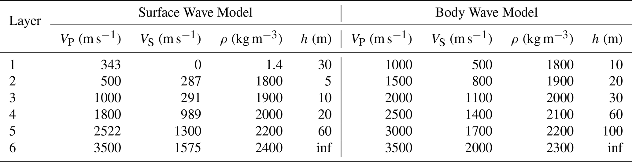
We validated our seismic wave propagation model using three distinct tests: body-wave imaging, surface wave dispersion analysis, and anisotropy/attenuation assessment. Each test was designed to benchmark the solver against expected physical phenomena in layered or anisotropic elastic media. Table (1) provides the isotropic velocity model for the surface wave and body wave focused simulations. Each of these models was tuned to present clear modes.

Table 1 Layer-wise P and S wave velocities and densities for surface and body wave models.

4.2.1 Surface Wave Excitation

To assess stability in the solver at high impedance boundaries as well as surface wave behavior and frequency-dependent phase velocity, we simulated a 6-layer stratified elastic half-space with low-velocity surface layers. Our source function was an accelerated weight drop broadband pulse that spanned 1.25–10 Hz located within the first subsurface layer at 4 m depth. Receivers were located at 1 m spacing and 1 m below the surface, with a total aperture length of 576 m. Figure 6a shows the resulting vertical component shot gather, dominated by dispersive Rayleigh mode surface waves propagating across the array.

Figure 6 Common shot gather (left) and the resulting multichannel analysis to highlight surface waves generated in the layered model in Table 1. The source is an accelerated weight drop at the surface with a multimodal wavelet that spans 3 octaves. The dominant fundamental mode R₀ up to the third mode R₃ are identified with theoretical dispersion curves overlain.

Figure 6b is a frequency–velocity (f–c) transformation from the shot gather with overlaying theoretical dispersion curves calculated using the disba package (Luu, 2021) in Python. Our implementation follows the general MASW framework proposed by Park et al. (1999), with energy imaging based on a slant-stack method McMechan and Yedlin (1981), and smoothed in the frequency–velocity domain. The results in Fig. 6b show clear dispersion branches and coherent energy for the fundamental mode (R₀) that has good alignment with simulated energy ridges. The fundamental mode is dominant to about 20 Hz at which point the first (R₁) and second (R₂) modes dominate the energy spectra. The theoretical dispersion curves were velocity shifted across all modes by −45 m s⁻¹ to match the synthetics. The slight velocity shift could be due to apparent velocities in the FDTD solver being lower than the analytical dispersion.

4.2.2 Body Waves

In order to emphasize body waves, we comprised a vertically stacked six-layer isotropic model with increasing velocity and density with depth. A 40 Hz Gaussian derivative point source was placed 10 m from the left boundary at a 3 m depth with 486 receivers at 1 m spacing. In order to avoid complexity in the wavefield, we intentionally excluded a free surface boundary condition and air layer to suppress surface wave excitation and associated ground roll. This creates a virtually infinite boundary which would also suppress body wave reverberations at the surface.

Figure 7 Common shot gather (left) for the six layer velocity model (Table 1), and the f–k analysis of the shot gather (right). Each time series is normalized using a 1200 point auto-gain control. The identified phase arrivals are labeled near their wavefronts using expected arrival times. Signal-to-noise ratios decrease rapidly causing boundary reflections to dominate later in the time series. The slopes of energy envelopes corresponding to specific velocities can be seen in the f–k plot for shear waves (red dotted) and pressure waves (blue dashed).

The velocity and density structure (Table 1) was selected to avoid artificial waveguides and suppress evanescent energy by minimizing sharp impedance contrasts at thin layers but also to permit clean observation of P and S body wave arrivals and their internal reflections, refractions, and conversions. The shot gather (Fig. 7a) exhibits clear PP, PS, and SP phases, as well as higher-order multiples and converted waves. The large aperture length of 486 m allowed for clear refracted shear (S_ref) and pressure (P_ref) waves to be observed for the top 3 velocity boundaries (layers 1–4). Reflected waves are shrouded in more noise and interference and harder to distinguish without more sophisticated processing.

The corresponding frequency-wavenumber analysis (Fig. 7b) confirms that the simulated energy is confined within the expected velocity range (500–3500 m s⁻¹; Table 1), consistent with theoretical limits imposed by the layered structure. The model's fidelity in capturing reflection travel times and conversion kinematics validates both the spatial discretization and time integration of the solver for short-wavelength elastic wave phenomena.

4.2.3 Seismic Anisotropy and Attenuation

Incorporating the full 21-component stiffness tensor introduces several numerical and conceptual challenges for seismic wave propagation modeling. Unlike isotropic or transversely isotropic formulations, the general triclinic stiffness tensor removes most symmetries, requiring all off-diagonal coupling terms to be explicitly computed and applied at each spatial location. This increases both computational load and storage requirements, as well as the complexity of accurately implementing the stress-strain update equations within the finite-difference time domain (FDTD) scheme. The full tensor also introduces strong shear-mode coupling, non-orthogonal polarization directions, and oblique energy partitioning, which can create mode conversions and apparent cross-component leakage that are difficult to distinguish from numerical dispersion or grid anisotropy. Small numerical errors or minor parameter inconsistencies can lead to non-physical instabilities, non-causal behavior, or failure to satisfy the strong stability conditions required for elastic FDTD.

To identify instability within the primary model domain or the CPML layer, we set up a simple single material domain using a velocity model for the primary crystal symmetries: hexagonal, orthorhombic, monoclinic, and triclinic. While monoclinic and triclinic media are not common to snow and ice, this represents an end member in the complexity of implementation but also shows that this is a highly generalized modeling routine. The maximum stable timestep for each material is determined using the full Christoffel eigenvalue solution, sampling multiple propagation directions to capture the maximum phase velocity arising from the full stiffness tensor. The maximum p-wave and shear wave velocities are matched throughout the different tensors to provide a point of reference and synchronization of energy entering the CPML boundary.

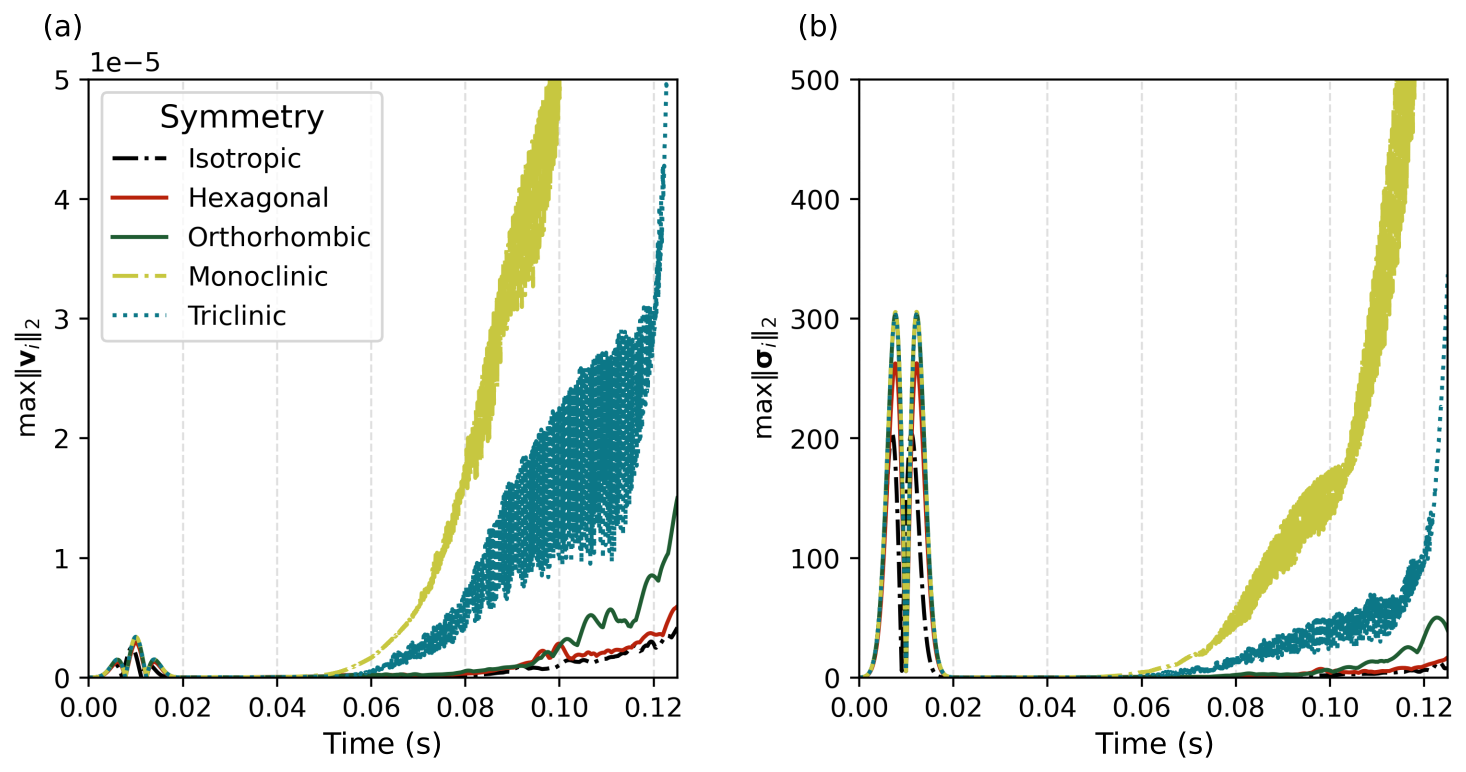
Figure 8 The temporal evolution of the maximum value of the velocity (left) and stress (right) field norms. This is not a full accuracy assessment but instead shows that the time window of the solver has a practical limit especially in the lower order symmetries.

Calculating the absolute maximums for the directional velocity and stress norms, we can see in Fig. (8) similar behavior identified by Bécache et al. (2003). For both the velocity (Fig. 8a) and stress (Fig. 8b) norms, instabilities begin to propagate soon after the slower shear modes enter the CPML. The theoretical first arrivals for the maximum P wave velocity and minimum shear wave velocity of 0.012 and 0.039 s, respectively. There is slightly more prolonged stability in the isotropic, hexagonal, and orthorhombic cases (diminishing in that order), but given enough time, numerical instabilities will dominate the signal. This shows limits to the capabilities of the model but also provides practical design considerations in order to model lower symmetry media. Lower symmetry allows more directions where the PML stretching is misaligned with the energy flux, which promotes numerical instability in the absorbing layer.

To verify that the anisotropic solver and CPML do not introduce grid-induced anisotropy, spurious mode coupling, or boundary artifacts, we calculated 3D polar velocity maps for an orthorhombic fabric. An explosive source was situated at the domain center, surrounded by 4824 receiver nodes forming a spherical shell at an omnidirectional radius of ≈47 m. To automate phase identification across the array, 3-component velocity traces ($v_x,v_y,v_z$) at each receiver were first transformed into ray-centered quasi-coordinates ($Q,\mathrm{SV},\mathrm{SH}$) using the Christoffel eigenvectors. From these rotated components, a moving-window rectilinearity R(t) was computed following Jurkevics (1988).

Phase arrival pick candidates are initially detected where rectilinearity drops below a defined threshold (R(t)≤0.8). To refine these arrival times, a discrete Akaike Information Criterion (AIC) picker (Takanami and Kitagawa, 1988; Akaike, 2003) is applied directly to the rectilinearity time series. The AIC approach models the signal as two locally stationary auto-regressive segments separated by an unknown onset point k. For a series x(t) of length N, the sample variances, r_i, before and after candidate split-point k are defined as:

$$\begin{array}{}\text{(67)}& r_{\mathrm{1}}\left(k\right)=\mathrm{Var}(x_{\mathrm{1}},\mathrm{\dots },x_k),r_{\mathrm{2}}\left(k\right)=\mathrm{Var}(x_{k+\mathrm{1}},\mathrm{\dots },x_N)\end{array}$$

The AIC function evaluates the objective score for each candidate index $k\in [\mathrm{1},N-\mathrm{2}]$:

$$\begin{array}{}\text{(68)}& \begin{array}{rl}& \mathrm{AIC}\left(k\right)=\\ & \left\{\begin{array}{ll}k\ln \left(r_{\mathrm{1}}\left(k\right)\right)+(N-k-\mathrm{1})\ln \left(r_{\mathrm{2}}\left(k\right)\right),& \text{if }{r}_{\mathrm{1}}\left(k\right)>\mathrm{0}\text{ and }{r}_{\mathrm{2}}\left(k\right)>\mathrm{0},\\ \mathrm{\infty },& \text{otherwise}\end{array}\right.\end{array}\end{array}$$

The optimal phase arrival sample $\widehat{k}$ minimizes the global log-likelihood function across the window:

$$\begin{array}{}\text{(69)}& \widehat{k}=\arg \underset{\mathrm{1}\le k\le N-\mathrm{2}}{min}\mathrm{AIC}\left(k\right)\end{array}$$

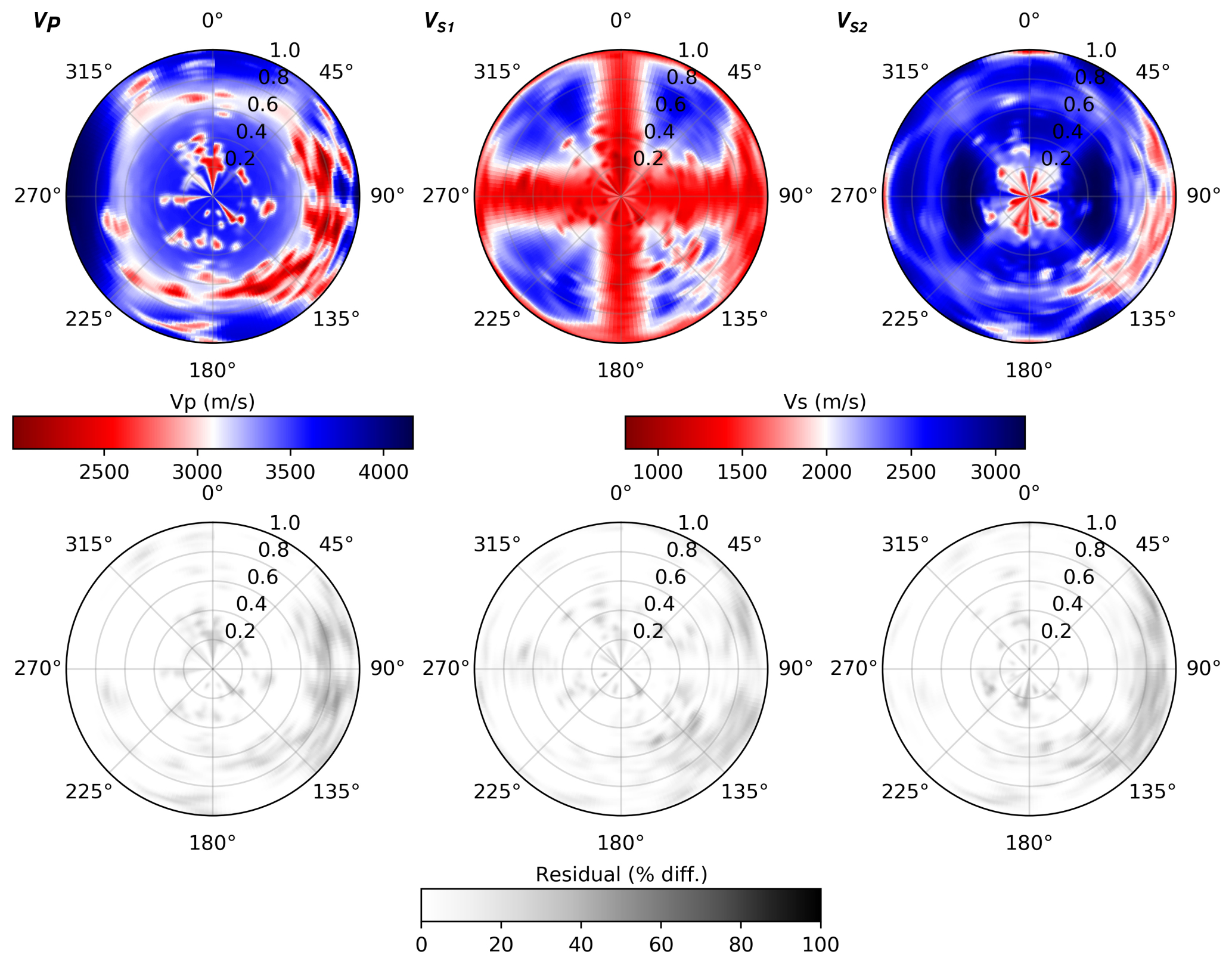
Figure 9 Polar azimuthal velocity maps for V_P, V_S1, and V_S2 (top row) as determined by auto-picked arrival times. The residual maps (bottom row) show an elevated but localized area of misfit. Overall, the auto-picker and wave speeds show good accuracy with expected anisotropic patterns.

For each phase and receiver, the velocity field ($v_x,v_y,v_z$) was transformed into ray-centered quasi-coordinates ($Q,\mathrm{SV},\mathrm{SH}$) using the Christoffel eigenvectors before calculating the rectilinearity. We then compute theoretical travel times from the Christoffel solution and form a final arrival time by taking the error-weighted mean of the polarization and AIC picks. Sharp drops in rectilinearity suggest phase arrivals, but interference from diffuse or stacked wavefronts can create more minima and less confidence. Therefore, search windows of 0.01 s were applied around the theoretical travel times with more weight towards the theoretical travel times when confidence was lower (rectilinearity ≥ 0.8) so that picks more consistent with the reference model contribute more strongly while still allowing both methods to influence the estimate.

Figure 10 The rectilinearity (a) computed from the 3-component rotated seismograms (b–d) with instantaneous power envelopes (gray fills) highlighting phase energy onsets. The source-receiver distance was increased to 105 m (compared to 47 m in Fig. 9) to resolve phase ambiguity. Theoretical arrival times for the quasi-P wave (t_P), fast shear wave (t_S1), and slow shear wave (t_S2) are indicated by vertical dashed lines.

To demonstrate this picking workflow, Fig. 10a illustrates how the moving-window rectilinearity tracks changes in particle-motion linearity as individual modes traverse the array. At the onset of the quasi-P wave (t_P≈0.029 s), rectilinearity drops below the 0.8 threshold, successfully triggering the automated P wave pick. Notably, residual quasi-P energy bleeds onto the Quasi-SV component (Fig. 10c), which likely stems from slight misorientation of the assumed phase normal during coordinate rotation. A secondary drop in rectilinearity occurs near t≈0.038 s, corresponding to the theoretical arrival of the fast shear mode (t_S1). Although the theoretical travel time for the slow shear mode (t_S2≈0.065 s) slightly underestimates the peak energy arrival, the true phase onset remains well within the designated search window.

The auto-picker doesn't perform perfectly and we can see the residuals between the auto-picked travel times and the theoretical travel times have a small percent differential in a compact angular wedge across the boundary of the 1st and 2nd quadrants of the residual map (Fig. 9) rather than along whole symmetry axes or mirrored quadrants. Since this radiation pattern does not reflect the material symmetry, we attribute these localized pick anomalies as being influenced by a combination of discrete grid geometry and the wavefront still being strongly curved. The receivers are only 1.5 wavelengths from the source so the wavefront is still far from planar and more sensitive to local discretization and staggering.

5 Summary and Conclusion

SeidarT provides a versatile, open-source framework for full-waveform modeling of both seismic and electromagnetic wave propagation in anisotropic, heterogeneous, and attenuating materials, with a particular emphasis on snow and ice environments. Through systematic validation – including comparison with experimental field results and analytical solutions – our implementation demonstrates robust accuracy in capturing key physical phenomena such as elastic and electromagnetic wave travel times, amplitude decay, and tensor-driven anisotropy effects.

The design philosophy of SeidarT reflects a deliberate choice to prioritize accessibility and extensibility over the absolute performance gains offered by more specialized implementations. By coupling the computational efficiency of Fortran with the user-friendly scripting capabilities of Python, we have created a software package that maintains high performance for time-critical simulations while remaining intuitive for rapid model development and iteration. The image-based geometry specification and JSON project workflow eliminate the need for complex, error-prone mesh generation routines – a significant barrier for many users transitioning from theoretical frameworks to practical numerical experiments.

The incorporation of empirically derived relationships for ice and snow material properties (permittivity, stiffness, density) ensures that synthetic models can be directly constrained by field observations, EBSD crystal orientation data, and laboratory measurements. The multiple homogenization schemes (Hill average, Gassmann substitution, Self-Consistent Approximation) provide flexibility to match effective medium assumptions to the microstructural regime, whether modeling consolidated ice, temperate snow with liquid water, or air-filled cavities. This adaptability is essential given the high variability of snow and ice properties across thermal and porosity regimes.

While our validation demonstrates the solver's capability across a range of scenarios, we acknowledge important limitations. The CPML absorbing boundary, though effective across most conditions, exhibits instabilities in lower symmetry (monoclinic and triclinic) materials at late times, as evidenced in our anisotropy tests (Sect. 4.2.3 and Fig. 8). This limitation, identified by Bécache et al. (2003) in the broader FDTD literature, stems from the misalignment of PML stretching with energy flux in non-orthogonal crystal systems. Parameter tuning strategies and explicit stability checks will provide the ability to model highly anisotropic materials but users should remain cognizant of practical time windows for reliable results.

There is ample room for future growth and performance optimizations; however, SeidarT was designed around community-driven development to bridge the gap between specialized academic research and commercial, proprietary software packages. It not only increases accessibility to advanced wave-propagation modeling but also enables the development of innovative approaches in geophysical imaging and subsurface characterization. We anticipate that as computing resources continue to expand and open-source collaboration grows, SeidarT will serve as a foundation for ever-richer simulations that link (micro)structural heterogeneity to macroscopic wavefield behavior.

Appendix A

Table A1 List of Symbols.

Appendix B: Zero Offset Profile

See Fig. B1 for the labeling of the layers as given in Table B1.

Table B1 The model parameters used to generate the zero-offset profile in Fig. 4.

^* The ID refers to the value in the figure and not in the JSON project file in the GitHub repository.

Figure B1 The annotated image of the model domain used to replicate the zero-offset profile in Fig. 4. The sources and receivers were located along a vertical profile to mimic the borehole profiling.

Appendix C: Seismic Anisotropic Parameters

The Python scripts and JSON project files can be found in the SeidarT-Recipes repository. The stiffness tensors used in these models are:

$$\begin{array}{lll}{\displaystyle }& {\displaystyle }\text{Isotropic}& {\displaystyle }\text{Hexagonal}\\ {\displaystyle }& {\displaystyle }\left[\begin{array}{cccccc}\mathrm{13.24}& \mathrm{6.62}& \mathrm{6.62}& \mathrm{0}& \mathrm{0}& \mathrm{0}\\ & \mathrm{13.24}& \mathrm{6.62}& \mathrm{0}& \mathrm{0}& \mathrm{0}\\ & & \mathrm{13.24}& \mathrm{0}& \mathrm{0}& \mathrm{0}\\ & & & \mathrm{3.31}& \mathrm{0}& \mathrm{0}\\ & & & & \mathrm{3.31}& \mathrm{0}\\ & & & & & \mathrm{3.31}\end{array}\right]& {\displaystyle }\left[\begin{array}{cccccc}\mathrm{14.57}& \mathrm{9.27}& \mathrm{3.86}& \mathrm{0}& \mathrm{0}& \mathrm{0}\\ & \mathrm{14.57}& \mathrm{3.86}& \mathrm{0}& \mathrm{0}& \mathrm{0}\\ & & \mathrm{14.57}& \mathrm{0}& \mathrm{0}& \mathrm{0}\\ & & & \mathrm{3.31}& \mathrm{0}& \mathrm{0}\\ & & & & \mathrm{3.31}& \mathrm{0}\\ & & & & & \mathrm{2.65}\end{array}\right]\\ {\displaystyle }& {\displaystyle }\text{Orthorhombic}& {\displaystyle }\text{Monoclinic}\\ {\displaystyle }& {\displaystyle }\left[\begin{array}{cccccc}\mathrm{13.24}& \mathrm{2.65}& \mathrm{1.99}& \mathrm{0}& \mathrm{0}& \mathrm{0}\\ & \mathrm{15.89}& \mathrm{2.32}& \mathrm{0}& \mathrm{0}& \mathrm{0}\\ & & \mathrm{11.92}& \mathrm{0}& \mathrm{0}& \mathrm{0}\\ & & & \mathrm{2.98}& \mathrm{0}& \mathrm{0}\\ & & & & \mathrm{3.31}& \mathrm{0}\\ & & & & & \mathrm{3.64}\end{array}\right]& {\displaystyle }\left[\begin{array}{cccccc}\mathrm{13.24}& \mathrm{2.65}& \mathrm{1.99}& \mathrm{0}& \mathrm{0}& \mathrm{0.36}\\ & \mathrm{15.89}& \mathrm{2.32}& \mathrm{0}& \mathrm{0}& \mathrm{0.36}\\ & & \mathrm{11.92}& \mathrm{0}& \mathrm{0}& \mathrm{0.36}\\ & & & \mathrm{2.98}& \mathrm{0}& \mathrm{0}\\ & & & & \mathrm{3.31}& \mathrm{0}\\ & & & & & \mathrm{3.64}\end{array}\right]\\ {\displaystyle }& {\displaystyle }\text{Triclinic}\\ {\displaystyle }& {\displaystyle }\left[\begin{array}{cccccc}\mathrm{13.24}& \mathrm{2.65}& \mathrm{1.99}& \mathrm{0.15}& \mathrm{0.17}& \mathrm{0.18}\\ & \mathrm{15.89}& \mathrm{2.32}& \mathrm{0.12}& \mathrm{0.13}& \mathrm{0.15}\\ & & \mathrm{11.92}& \mathrm{0.09}& \mathrm{0.10}& \mathrm{0.01}\\ & & & \mathrm{2.98}& \mathrm{0.60}& \mathrm{0.60}\\ & & & & \mathrm{3.31}& \mathrm{0.66}\\ & & & & & \mathrm{3.64}\end{array}\right]\end{array}$$