Seasonal icings reveal subsurface water drainage of a Greenland Ice Sheet outlet glacier

In many glacial settings, winter outflows of proglacial water create stratified domed ice structures on glacial forefields. These structures, called naledi, provide an opportunity to characterise solute concentrations in hydrological systems during winter, which are poorly constrained compared with summer outflows dominated by supraglacial meltwater. To characterise the different hydrological systems feeding naledi and provide conceptual models of their formation, we sampled 12 overwinter naledi and 4 summer ice accumulations (accreted ice) from the forefield of Isunnguata Sermia, a western outlet glacier of the Greenland Ice Sheet, during four field campaigns. Major ions and stable water isotopes reveal complex geochemical signatures, where the composition of successive naled layers indicates fluctuations in water source and transport throughout winter. In comparison, summer accreted ice is sediment laden and shows uniform geochemistry throughout, suggesting freeze-on of water from a single source in quick, discrete events. These findings are supported by Electrical Resistivity Tomography (ERT) geophysical surveys showing shallow hydrological pathways (1–5 m below the surface) in the glacial foreland (surveyed 400 m from the glacier terminus). These results inform the first conceptual models of summer vs. wintertime subglacial water routing and naled formation in the proglacial zone of the Greenland Ice Sheet. We show that wintertime naledi form from a combination of top-down (unconfined) and bottom-up (confined) freezing processes incorporating subglacial discharge, overland flow and precipitation. In contrast, accreted ice forms from upwellings of high-velocity, highly pressurised water which freezes upon release. These seasonal changes drive different geochemical and solute outputs, which are critical for evaluating glacier meltwater contributions to proglacial groundwater systems and the impact of glacial discharge on downstream ecosystems.

1 Introduction

The Greenland Ice Sheet is a major exporter of biologically important elements to the world's oceans (Hawkings et al., 2016; Lawson et al., 2014; Wadham et al., 2016) and a hotspot for CO₂ drawdown through chemical weathering processes (Graly et al., 2017; Pain et al., 2021). Most of our knowledge of chemical and biological fluxes from the Greenland Ice Sheet comes from analysis of the summer ablation season outflow, where channelised melt waters contact only a limited portion of the glacier bed (Bhatia et al., 2013; Hawkings et al., 2016; Meire et al., 2016; Yde et al., 2014). However, during winter, outflow is typically fed by slower-flowing subglacial meltwater, which has often been subjected to greater contact time with the ice/bed interface (Chandler et al., 2013; Davison et al., 2019). As there are inherent challenges associated with field sampling subglacial water flow over winter, there is limited inclusion of winter water in geochemical modelling, inhibiting our understanding of year-round subglacial weathering processes and nutrient export from Greenland.

In many proglacial environments in the Arctic, domed ice structures called naledi (singular naled but also referred to as aufeis or icings) develop within glacier forefields in the winter months (Carey, 1973; Hodgkins et al., 2004; Mallinson et al., 2019; Morse and Wolfe, 2015; Sobota, 2016; Yoshikawa et al., 2007). These naledi typically consist of stratified layers of frozen subsurface and subglacial water discharged over winter (November–March). As such, they provide a potential source for characterising wintertime solute concentrations and insights into chemical weathering processes operating over low-flow hydrological conditions that are difficult to obtain by other means. Layers build up over winter to produce a domed, layered, ice structure, which can reach multi-metre heights, forming where outflows of water are expelled in discrete locations of the glacial foreland and quickly freeze due to low air temperatures (Harden et al., 1977; Kane, 1981).

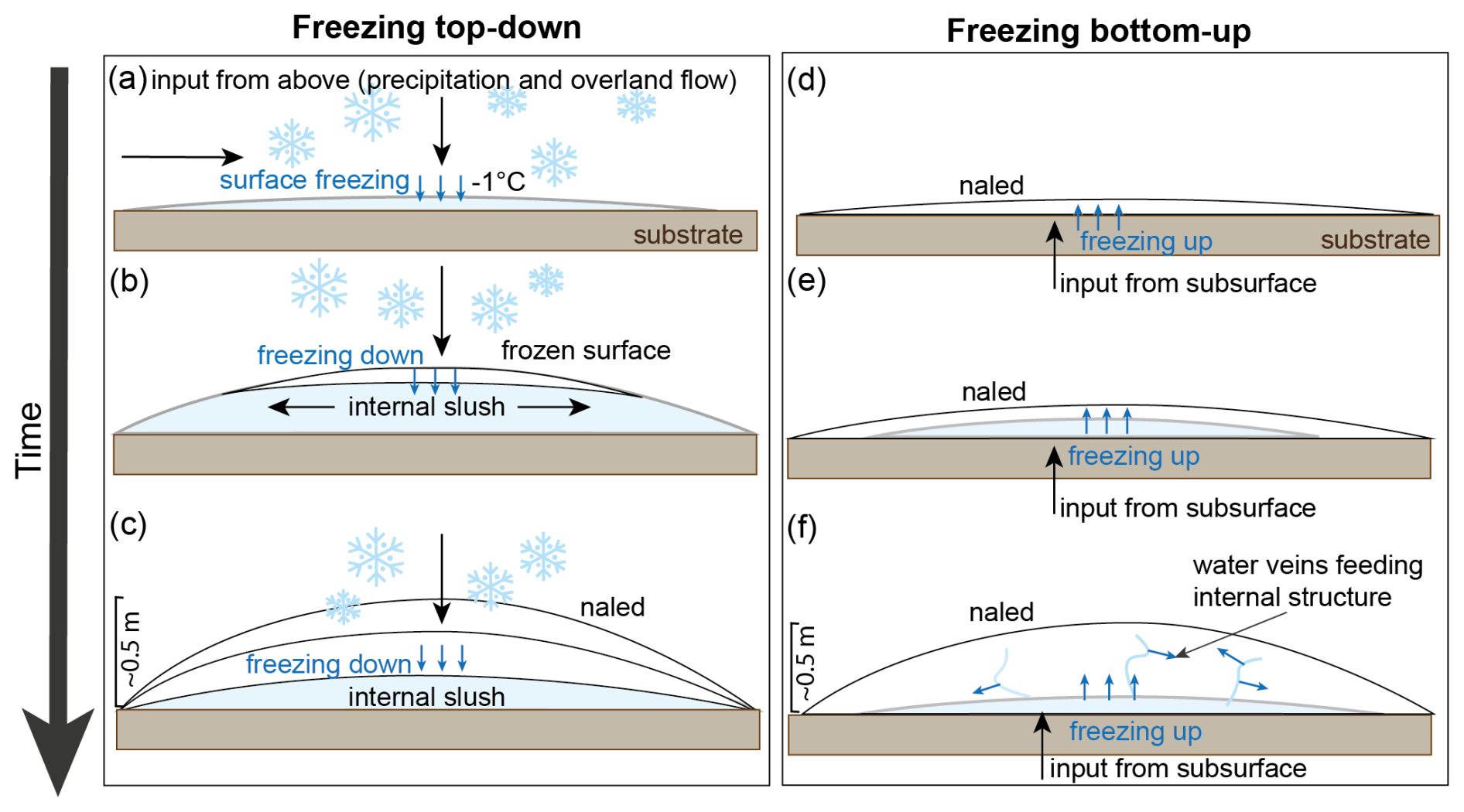
Figure 1 Prevailing theories of naled ice formation. (a–c) A top-down freezing process by which overland flow and precipitation freeze at the surface due to subzero air temperatures (Schohl and Ettema, 1986). (d–f) A bottom-up freezing process by which subsurface waters erupt into the forefield and freeze from the base-up, with newly erupting waters accreting onto the bottom of the naled. In these bottom-up models, there is also potential for small water veins within the naled to accrete ice within (Wadham et al., 2000; Stachnik et al., 2016).

The prevailing theoretical models of naled formation, established ∼ 40 years ago, suggest that naled grow in a top-down fashion because the cold winter atmosphere acts as a heat sink, freezing unconfined waters that accumulate from above (Fig. 1a–c) (Schohl and Ettema, 1986; Yde et al., 2012). However, more recent and direct observations of proglacial naled in Svalbard by Stachnik et al. (2016) interpreted naled formation as a primarily bottom-up process. This theory suggests new meltwaters confined below ice push up older, frozen layers (Fig. 1d–f), and that liquid water conduits within naled ice provide insulated transport pathways, protected from the cold surface (Fig. 1f). These contrasting models of formation make it challenging to extrapolate general chemical and biological insights into different hydrological systems.

In previous research, principally on Svalbard, the chemistry preserved in naled ice has been successfully characterised by analysing ice cores collected in early spring (Stachnik et al., 2016; Wadham et al., 2000; Yde et al., 2012). These studies found that the overwinter solute flux captured in naled differs significantly from the early spring or late summer meltwater output from glacial systems, suggesting they can capture a distinct wintertime hydrochemical regime (Graly et al., 2018). However, complexity in their geochemistry indicates multiple water source inputs may build up a single naled (Yde et al., 2012) with chemical differences between different ice layers (Stachnik et al., 2016). The glaciers of Svalbard represent relatively small glacier hydrologic systems, with small storage capacities compared to larger ice sheets, like the Greenland Ice Sheet and its outlet glaciers (Wadham et al., 2000). It is therefore possible that the chemical signatures of naled ice in these larger systems may represent different formation mechanisms than those in Svalbard. In glacial foreland areas, supercooled waters can also freeze and build up accreted ice structures over summer, often during high discharge events sourced from glacial overdeepenings that are heavily sediment-laden (Alley et al., 1998; Evenson et al., 1999; Lawson et al., 1998; Roberts et al., 2001; Roberts et al., 2002; Livingstone et al., 2026).

Here, we measure and interpret the chemical characteristics and identify the sources of water creating wintertime naled ice and summertime accreted ice in the forefield of Isunnguata Sermia on the western Greenland Ice Sheet. We combine our geochemical analyses with geophysical surveys of the forefield to assess potential routing mechanisms of water flow feeding these structures and explore seasonal changes in the hydrological system. Our results inform a new conceptual model of naled and accreted ice formation applicable to similar proglacial systems in West Greenland and other glaciated regions.

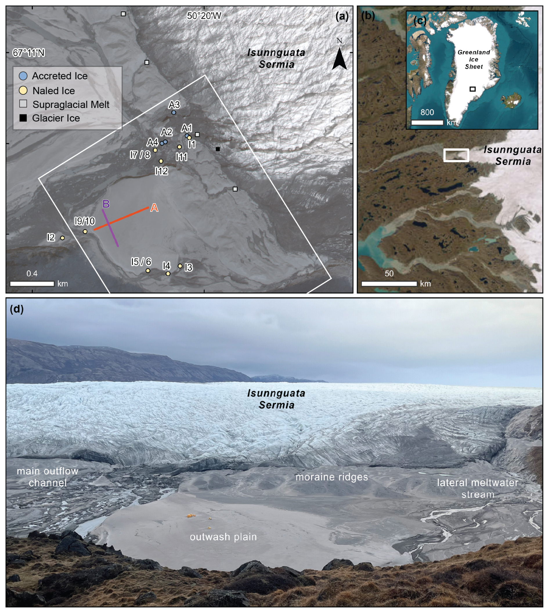
Figure 2 Isunnguata Sermia field site in West Greenland (a) Location of sampling sites, geophysical survey transects (A and B) and camera trap locations in the forefield of Isunnguata Sermia. White box denotes the photograph area shown in panel (d). (b) Sample area of the Isunnguata Sermia forefield (white box), where meltwater is exported from the Greenland Ice Sheet (c). (d) Overview photograph of the proglacial forefield from May 2023 with key sites annotated. The yellow features on the outwash plain are camp tents, approximately 1.6–1.9 m high. Imagery © (2024) Vantor in panel (a) sourced from the Polar Geospatial Centre (showing June 2022) whilst panels (b) and (c) show Esri basemap imagery | Powered by Esri.

2 Study site

Isunnguata Sermia (67°11^′06.0^′′ N 50°20^′21.8^′′ W) drains ∼ 15 900 km² of the Greenland Ice Sheet and is located approximately 100 km away from the coast (Fig. 2) (Lindbäck et al., 2015). The outlet glacier is located in the central west region of Greenland, routed through an overdeepened bed (extending to ∼ 350 m below sea level) for over 20 km (Lindbäck et al., 2015). Throughout its catchment area, Isunnguata Sermia is expected to flow over granodioritic gneisses and associated silicate rocks of the Nassuttooqidian Orogen, a large-scale fold-belt formed ca. 2.7 billion years ago (van Gool et al., 2002).

Previous work has characterised spring/summer runoff and subglacial hydrology at Isunnguata Sermia (Bartholomew et al., 2011; Meierbachtol et al., 2013) as well as subglacial discharge and hydrochemistry of summer outflows (Graly et al., 2017). Wintertime outflow was chemically profiled by Pitcher et al. (2020), who sampled proglacial river water while performing local radar surveys of Isunnguata Sermia. This revealed that basal water is persistent at Isunnguata Sermia, discharging small amounts of water into the proglacial river system year-round. Isunnguata Sermia also sits on a reverse gradient bed slope with an active subglacial lake system (Livingstone et al., 2019). These lakes, located beneath the ablation zone of Isunnguata Sermia, have been shown to exhibit multi-year water storage, resulting in long water residence times, though research has also shown that meltwater can be quickly released during flood events (Chu et al., 2016; Livingstone et al., 2019).

The forefield of Isunnguata Sermia contains several discrete upwellings of subglacial water. These waters may emerge slowly, or as geyser-like features that expel water into the air on a metre- to multi-metre scale (Livingstone et al., 2026). In February 2015, supercooled water was discovered below the clear ice of a proglacial outlet stream, 1 km downstream of the Isunnguata Sermia terminus (Pitcher et al., 2020). This slow meltwater drainage, fed by the deeply incised subglacial trough that extends inland from the terminus (Graly et al., 2017), suggests that the local geometry might drive proglacial upwellings of subglacial meltwater year-round. As a result, this site provides an ideal location to investigate the geochemical signature of water sources feeding naled ice and accreted ice, allowing us to examine changes in hydrological pathways and fully characterise the chemical signature of year-round outflows, for the first time.

3 Methods

3.1 Automatic cameras

Monitoring of glacier outflow and the development of naledi was done by setting up time-lapse cameras (LTL-6210MC Plus Scouting Cameras) across the glacier forefield and monitored between 2022 and 2024 (Fig. 2 and Table S1 in the Supplement). Cameras were set up at six different locations and orientations to capture changes in the main outflow channel of Isunnguata Sermia and to review active upwellings at the time of installation. Photographs were taken at 11:00 am, 12:00 pm, 01:00 pm and 02:00 pm (local time) each day. Full descriptions of camera installations and observations can be found in Table S1.

3.2 Sampling

Four field campaigns were conducted to collect a representative sample set of ice and water samples across the Isunnguata Sermia forefield over multiple years both pre- and post-melt season (Fig. 2). We focused on three different sample types (i) naled ice (dome shaped structures, formed over winter likely during low discharge), (ii) naled waters upwelling in the outwash plain (capturing active water sources feeding naled ice over the winter months) and (iii) accreted ice (sediment-laden ice structures associated with active upwellings in the summer months) (Fig. 2).

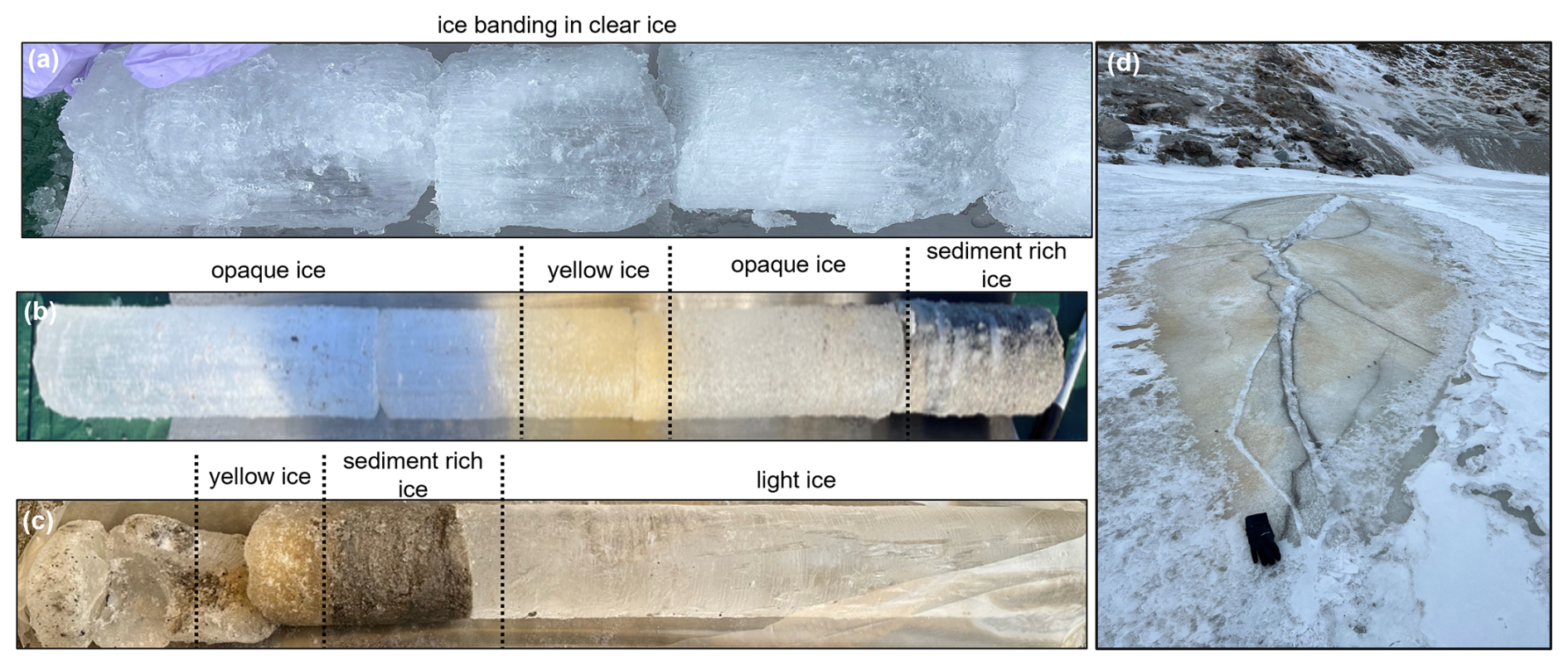
Figure 3 Naled ice structures and examples of different ice facies from cores. (a) Core I3 (15 cm), (b) upper 90 cm of core I10 and (c) lower 68 cm of core I10, as well as a photograph of a naled structure (cored for I10) (d) where a black glove (∼ 20 cm in length) is provided for scale.

Over the course of four field campaigns (October 2022, April 2023, September 2023 and March–April 2024), we sampled 12 naledi and 4 accreted ice structures (Figs. 2a and S1, S2 in the Supplement). Ice cores were extracted with a motorised SIPRE Auger to a maximum depth of 2 m. Cores were logged immediately, then sectioned by changes in ice facies and transported in individual sterile Whirl-Pak bags (Fig. 3). Core sections were then melted in a gently heated water bath in the field (less than 4 h after sampling) and filtered using Whatman 0.45 µm cellulose membrane filters into centrifuge tubes for major ion analysis. All samples were refrigerated and stored at 3–4 °C until analysis. Four of the naled ice cores terminated in water sources. Cores at the other seven sites did not reach water and were limited to depths between 8 and 139 cm, often due to thick gravel deposits which rendered further drilling impossible.

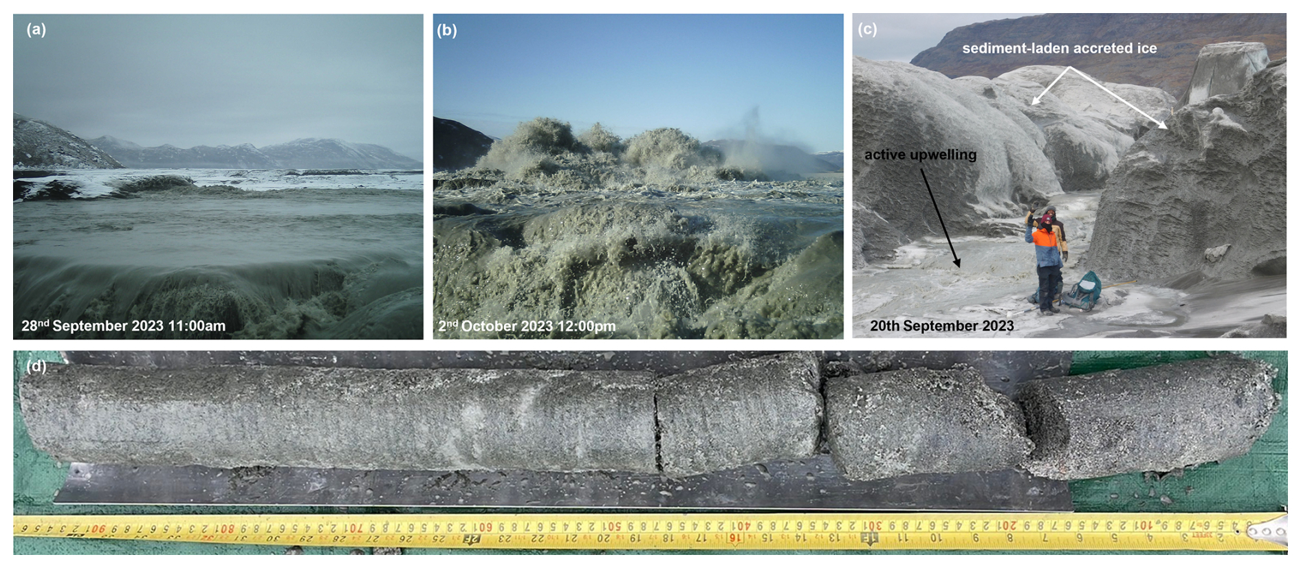
Figure 4 (a, b) Examples of a subglacial water outburst from Isunnguata Sermia, captured by automatic camera 4 in late September to early October 2023. Photographs show high water flow volumes on the 28 September (a) followed by an erupting outflow 4 d later (b). (c) Example of a multi-metre high accreted ice structure, alongside an active, bubbling upwelling of water, reviewed by field researchers on the 20 September 2023. (d) Example of a sediment-rich core from an accreted ice structure.

Of the cores that reached active water sources, naled I8 was located at the margin of the main meltwater channel and the three others (I2, I3 and I10) in an adjacent lateral meltwater stream (Fig. 2). In each case, samples of the naled upwelling waters were collected in sterile 50 mL centrifuge tubes and filtered using Whatman 0.45 µm nylon membrane filters. Accreted ice cores were sampled around the glacier front and within the main active frozen meltwater channel area in October 2022 (n=4, Figs. 2a, 4 and S3 in the Supplement). Unlike the naled ice core sites, none of the accreted ice cores reached free-flowing waters.

Contextual samples of glacier ice (n=2) and supraglacial meltwater (n=7) were also collected to represent end-member water types. Glacier ice was sampled from the upper ice margin of Isunnguata Sermia in April 2024 using a chisel and hammer, with the upper 10 cm layer of ice discarded to remove the outer layer of weathered ice (Fig. 2a). Supraglacial water was sampled from the ice margin and atop the Isunnguata Sermia glacier snout in 50 mL centrifuge tubes.

3.3 Geochemistry

Concentrations of major anions in water and melted ice samples were analysed in triplicate on a Dionex Integrion high-pressure ion chromatography (IC) system at Northumbria University using 5 mL of sample. Standard solutions of fluoride (F⁻), chloride (Cl⁻), sulphate (${\mathrm{SO}}_{\mathrm{4}}^{\mathrm{2}-}$), and nitrate (${\mathrm{NO}}_{\mathrm{3}}^{-}$) were prepared using 18.2 MΩ ultrapure water to obtain standard curves. Concentrations of major cations were analysed in triplicate on an Optima 8000 inductively coupled plasma optical emission spectrometer (ICP-OES) at Northumbria University using 7 mL of sample. Standard solutions of calcium (Ca), potassium (K), magnesium (Mg), and sodium (Na) were prepared using ultrapure water to obtain standard curves. Limits of detection (LOD) for both instruments was determined by standard regression on the intercept of the calibration curve and measured 0.02 mg L⁻¹. Analytical precision was assessed as the relative standard deviation (RSD %) of triplicate measurements for each sample. RSD was below 3 % for all analytes and across all run days for the ICP-OES and the IC, indicating good analytical reproducibility. ${\mathrm{HCO}}_{\mathrm{3}}^{-}$ was then calculated using the charge balance error (CBE) method, where ϵ⁺ and ϵ⁻ are total cation and anion equivalents. Uncertainty in ${\mathrm{HCO}}_{\mathrm{3}}^{-}$ concentrations is derived from uncertainties of all measured cation and anion concentrations.

3.4 Stable water isotopes

Aliquots of samples were analysed for their hydrogen and oxygen isotopic composition using a Picarro L2130-i cavity ringdown spectrometer at Northumbria University. Four calibration standards were measured at the beginning of each run (including in-house laboratory standards supplied and calibrated by the University of Bergen (“EVAP-2”, “FINSE”, “GLW”) and international standard SLAP2 (Standard Light Antarctic Precipitation 2). Separate aliquots of reference water “Medium Natural Water” or “Greenland Water” (purchased from Elemental Microanalysis Ltd.) were analysed every 10 to 15 samples to monitor and correct instrument drift. Results were corrected for memory and drift and normalised to the VSMOW-SLAP (Vienna Standard Mean Ocean Water – Standard Light Antarctic Precipitation) scale, using the FARLAB Liquid Water Isotope Measurement Processor (FLIIMP) software package (Sodemann et al., 2023). No humidity correction was applied (following Weng et al., 2020). The drift standards (as well as one aliquot of VSMOW2 per run) were used as data quality monitors. Analytical error is equal to or better than 0.4 ‰ for δD and 0.07 ‰ for δ¹⁸O (SE); overall reproducibility based on monitor standards is equal to or better than 1.0 ‰ for δD, and 0.38 ‰ for δ¹⁸O (SD) (Table S2 in the Supplement). Individual “freezing packages”, which are discrete isotopic units within the naled ice body representing a temporally distinct episode of water upwelling and subsequent freezing at the ice surface, were also identified by calculating freezing curves for each ice core. In the context of refreezing Greenland Ice Sheet waters, a δD:δ¹⁸O slope of around 6 would be expected. The composition of the source water can be calculated from the two-isotope slope (Souchez and Jouzel, 1984), allowing us to determine the isotopic composition of the source water where a freezing slope is identified.

3.5 Electrical Resistivity Tomography

A SuperSting R8 eight-channel earth resistivity metre (Advanced Geosciences, Inc.) was used to investigate subsurface conditions and potential water transport routes through the forefield of Isunnguata Sermia (Fig. 2) in April 2024. The frozen ground had to be prepared for electrode stake deployment by thawing small areas to a depth of ∼ 30 cm using boiled water, heated from locally sourced snowmelt. A mixture of locally sourced glacial clay and salt or isotonic powder (Gatorade™) was poured over the thawed ground to secure each electrode stake and ensure sufficient ground coupling once the electrodes froze in. Fifty-six electrodes were installed in a forward and reverse dipole-dipole configuration along profile A with the same configuration along profile B (Fig. 2) for 47 electrodes. The maximum source current was set to 50 mA for both profiles, and electrode contact resistance was monitored throughout. All data were processed and inverted using ResIPy v3.6.3 (Blanchy et al., 2020) (see Supplement).

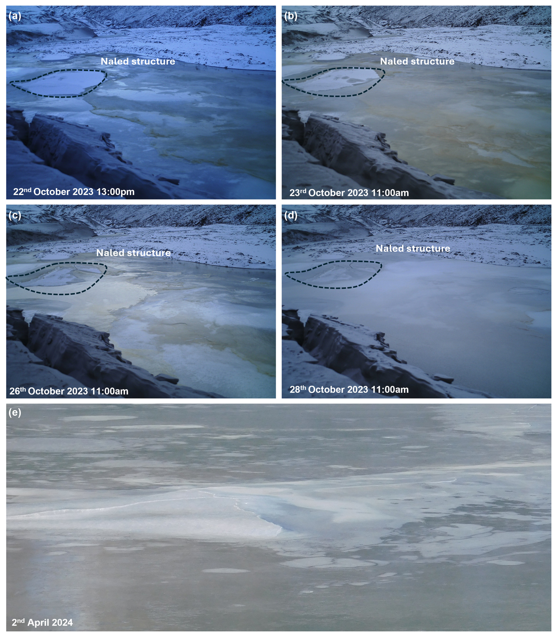
Figure 5 Upwelling of glacial waters in the forefield of Isunnguata Sermia, captured by an automatic camera installation (Camera 5) for the 2023/2024 winter season (a–d). Over the course of 6 d, distinctly yellow-coloured water flows and ice accumulations were recorded, suggesting variable water/snow inputs/throughputs. (a) Photograph showing the first emergence of yellow-coloured water in the glacial foreland. (b) The yellow outflow completely covers the proglacial river in the field of view. (c) White ice and snow begin to overlay the yellow layer, which has frozen. (d) The yellow ice layer is fully covered with fresh white ice and snow. Black dashed outline highlights the naled ice area. (e) A naled dome formed in the centre of the proglacial stream overnight on the 2 April 2024, captured in field photographs.

4 Results

4.1 Automatic cameras and Field Photos

Automatic cameras captured active naled and accreted ice formation as well as changes in winter outflow over the foreland of Isunnguata Sermia from 2022 to 2024. In 2023, Camera 5, orientated on the proglacial outwash plain facing the ice margin, captured the formation of winter-accumulating naled ice and an outflow of yellow-coloured water on the 22 October when the rest of the meltwater channel was frozen (Fig. 5). The source of flow from this yellow water originate from a location off-camera. The distinct colouration of this water can be seen freezing over the channel and naled structure over 3 d, before being covered by fresh snow on 28 October. These accumulation patterns suggest that similar ice layering may be expected in the naled icings.

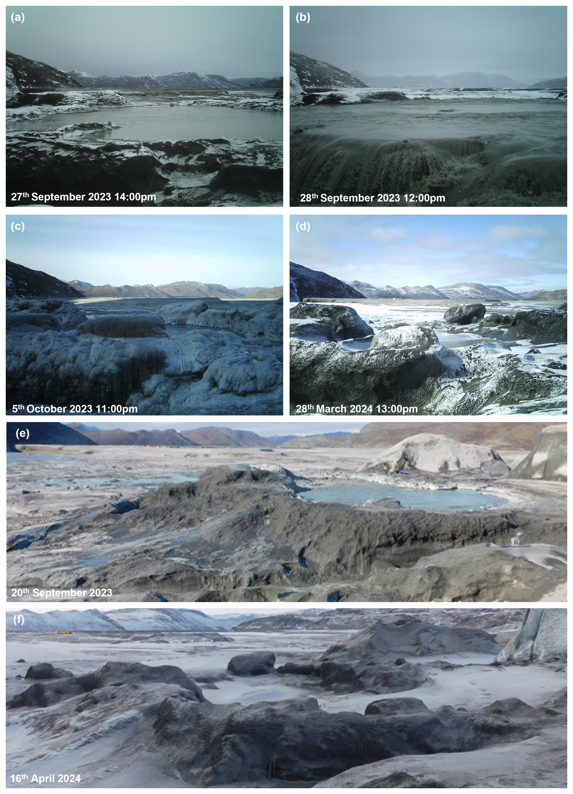
Figure 6 Accreted ice formation (a–d) captured by an automatic camera installation for the 2023/2024 winter season. (a, b) Over the course of a week an eruption of glacial meltwater occurred in the main proglacial meltwater channel close to the Isunnguata Sermia ice margin (Livingstone et al., 2026), see https://vimeo.com/manage/videos/1103612163 (last access: 1 April 2026). (c) This resulted in the rapid accumulation of ice accretions around the upwelling. (d) Over 6 months later, some ice persists around the upwelling source, preserved by the cold winter temperatures, though the ice structure appears deflated and eroded. A similar process is seen in (e), where sediment-rich ice accumulations around an upwelling site in late September 2023 had deflated and eroded substantially (f) the following April 2024.

A glacial outburst flood from Isunnguata Sermia was also detected between September and early October 2023 (see Livingstone et al. 2026). By analysing footage from two separate automatic cameras and orientations (see Supplement), a gradual increase in water levels of the main meltwater channel was observed before a vigorous outburst flood event on 2 October (Fig. 4a and b). We also observed the sudden build-up of sediment-laden accreted ice around the upwelling during the outburst event (Fig. 6). Much of the resulting accreted ice structure persisted up to 6 months later, preserved by the cold winter temperatures, though it appeared to have eroded, suggesting some melt wastage had occurred.

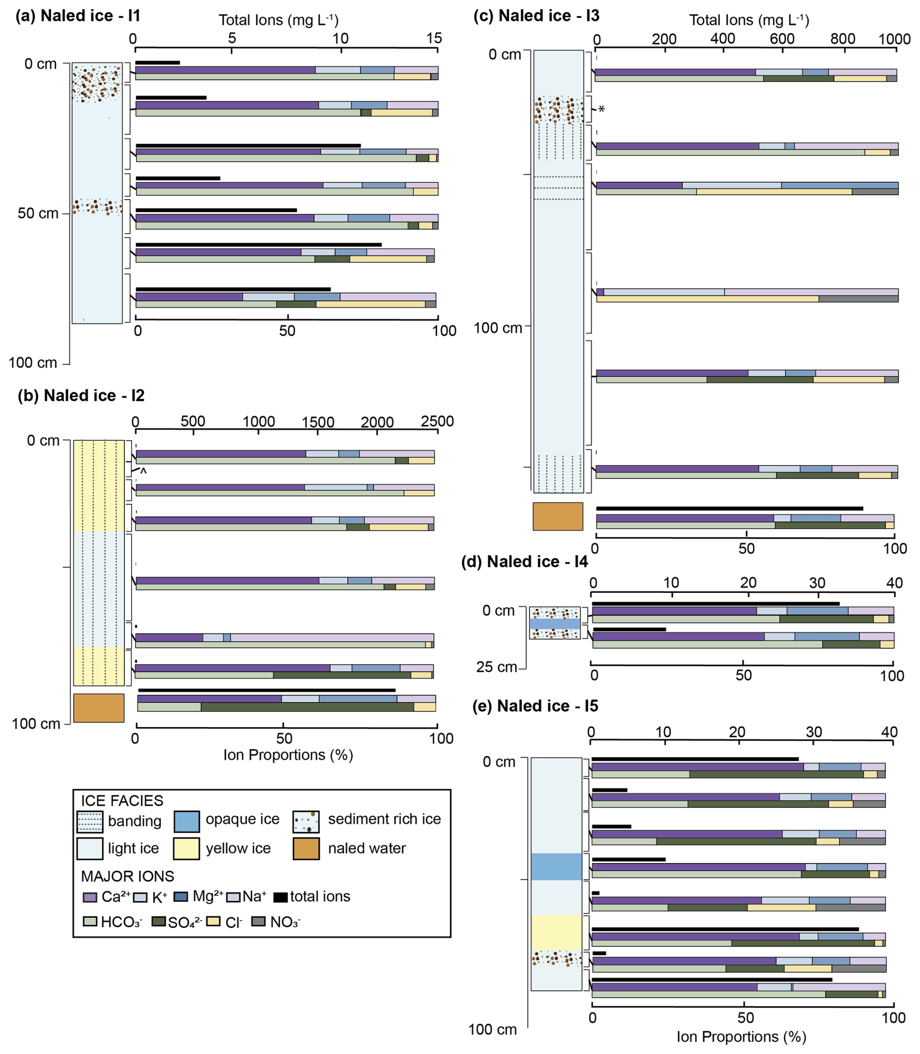
Figure 7 Ice facies and geochemical profiles of major ions for naled ice cores I1 through I5 collected April 2023 and March–April 2024. Vertical columns indicate ice facies types. Geochemical results are illustrated with cumulative horizontal bars adjacent to sampling depth (exact depth range indicated by black brackets). Total dissolved solids (TDS) are given in mg L⁻¹ (upper, black bar); note unique axis values for each core. For some samples, values are so low that they plot as a point. The proportions of cations (middle bar plot, Ca²⁺, K⁺, Mg²⁺, and Na⁺) and anions (lower bar plot, Cl⁻, ${\mathrm{SO}}_{\mathrm{4}}^{\mathrm{2}-}$, ${\mathrm{NO}}_{\mathrm{3}}^{-}$, and ${\mathrm{HCO}}_{\mathrm{3}}^{-}$) are given in percentages.

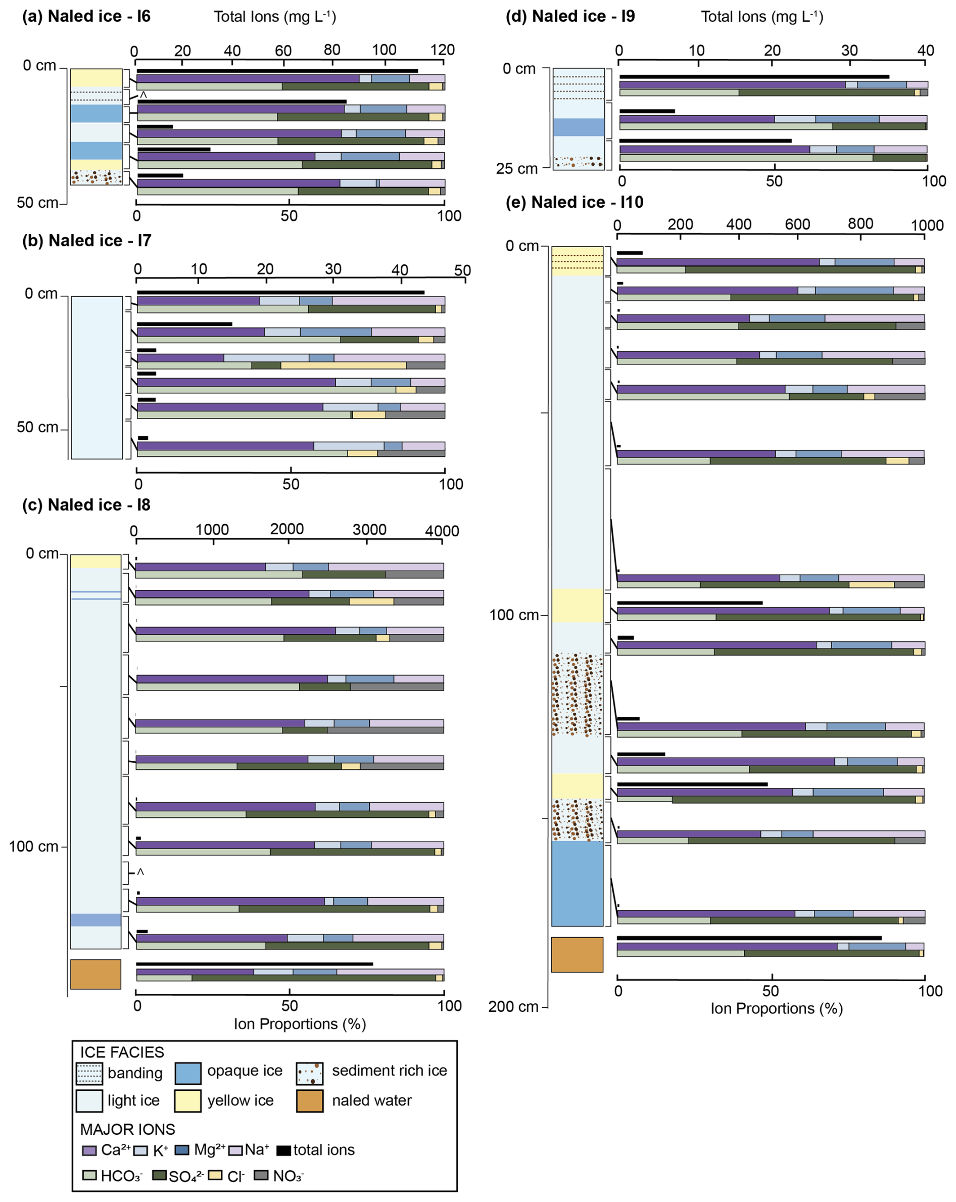
Figure 8 Ice facies and geochemical profile of major ions for naled ice cores I6 through I10 collected March–April 2024. Vertical columns indicate ice facies types and changes with depth. Geochemical results are illustrated with cumulative horizontal bars adjacent to sampling depth (exact depth range indicated by black brackets). TDS is given in mg L⁻¹ (upper bar; note unique charge range for each core) and the proportions of cations (middle bar plot, Ca²⁺, K⁺, Mg²⁺, and Na⁺) and anions (lower bar plot, Cl⁻, ${\mathrm{SO}}_{\mathrm{4}}^{\mathrm{2}-}$, NO³⁻, and ${\mathrm{HCO}}_{\mathrm{3}}^{-}$) are given in percentages.  Sample not analysed.

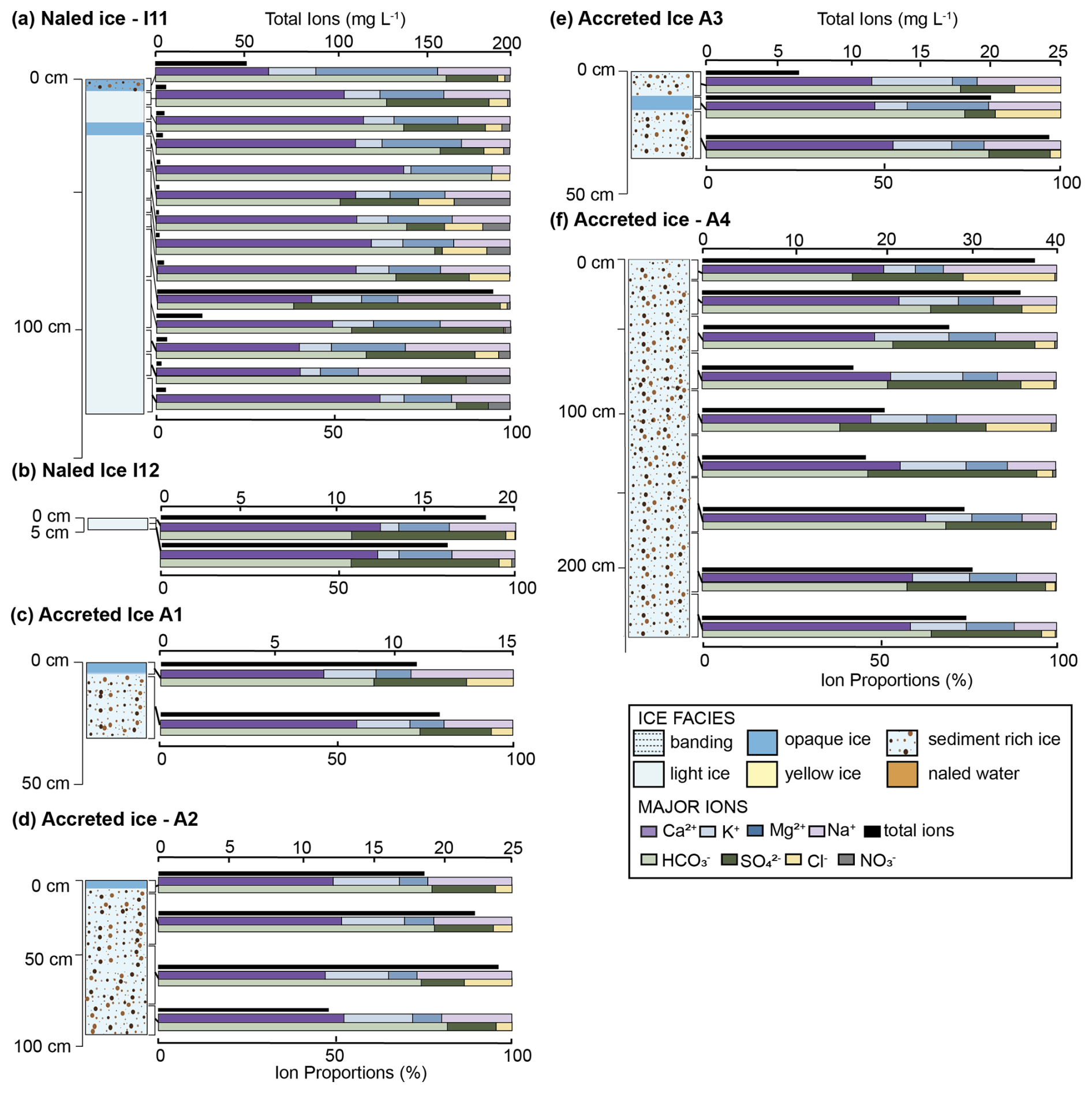
Figure 9 Ice facies and geochemical profile of major ions for naled ice cores I11 and I12 collected March–April 2024, and accreted ice cores collected October 2022 and April 2023. Vertical columns indicate ice facies types and changes with depth. Geochemical results are illustrated with cumulative horizontal bars adjacent to sampling depth (exact depth range indicated by black brackets). TDS is given in mg L⁻¹ (upper bar; note unique charge range for each core) and the proportions of cations (middle bar plot, Ca²⁺, K⁺, Mg²⁺, and Na⁺) and anions (lower bar plot, Cl⁻, ${\mathrm{SO}}_{\mathrm{4}}^{\mathrm{2}-}$, ${\mathrm{NO}}_{\mathrm{3}}^{-}$, and ${\mathrm{HCO}}_{\mathrm{3}}^{-}$) are given in percentages.

4.2 Ice facies analysis

Ice cores revealed distinct ice facies, which we group into four classifications: light ice, opaque ice, yellow-coloured ice, and sediment-rich ice (Fig. 3). Some ice has either horizontal or vertical stripes – which are more visible in the “light ice” and “opaque ice”. Light ice and opaque ice packages do not have sediment inclusions or discolouration, with the light ice mostly translucent and the opaque white or “clouded”, and were combined for geochemical analysis as “clear ice” for simplicity. Yellow-coloured ice was distinctly yellow in colour and appeared as discrete layers within the naled cores. Five ice cores recorded these yellow-coloured ice layers, which ranged in thickness from 10–25 cm, at various depths (Figs. 7b, e and 8a, c, and e). Yellow-coloured ice was not found in any of the accreted ice cores. Sediment-rich ice had clear sediment inclusions that accounted for > 50 % of the core section. Sediment layers were present in nearly all core samples (except I2, I7 and I8), with more pronounced sediment-rich layers (between 10–40 cm thick) recorded in I1, I3, I5 and I10 (Figs. 7 and 8). These sediment-rich layers only appeared as discrete layers within the naled cores, but they account for almost the full core length in the accreted ice cores (Figs. 3 and 4). Facies logs for each ice core and their resultant geochemical profiles are provided in Figs. 7–9.

Accreted ice cores were typically multi-metre in length and consisted of heavily sediment-laden ice (Fig. 4), which appeared to be a mix of frazil ice and silt to fine sand sediments. Cores ranged in length from ∼ 25 to 240 cm (Fig. 9). The longest core, A4, had no visible layers, but the full core was sediment-laden with clay to fine sand-sized particles (Fig. 4d). Bands of opaque ice, less than 10 cm thick, were recorded at various intervals throughout cores A1, A2 and A3.

4.3 Geochemistry

Proportions of major ions and total dissolved solids (TDS) are shown for each core in Figs. 7–9. The naled ice cores and their sub-naled waters display a range of TDS concentrations, broadly spanning from very dilute (less than 1 mg L⁻¹) to highly concentrated (up to 3000 mg L⁻¹) depending on the core and depth. Across most cores, ${\mathrm{HCO}}_{\mathrm{3}}^{-}$ is the dominant anion, while Ca²⁺ is consistently the most abundant cation. In general, we observe that ice layers with low TDS, such as naled I1 and lower I7 (Figs. 7a and 8b), are typically ${\mathrm{SO}}_{\mathrm{4}}^{\mathrm{2}-}$ poor (though sometimes ${\mathrm{NO}}_{\mathrm{3}}^{-}$ enriched). Whereas very concentrated TDS such as the naled waters in I2 and I3 (Fig. 7b and c) are more often ${\mathrm{SO}}_{\mathrm{4}}^{\mathrm{2}-}$ enriched and have higher TDS concentrations than the overlying ice.

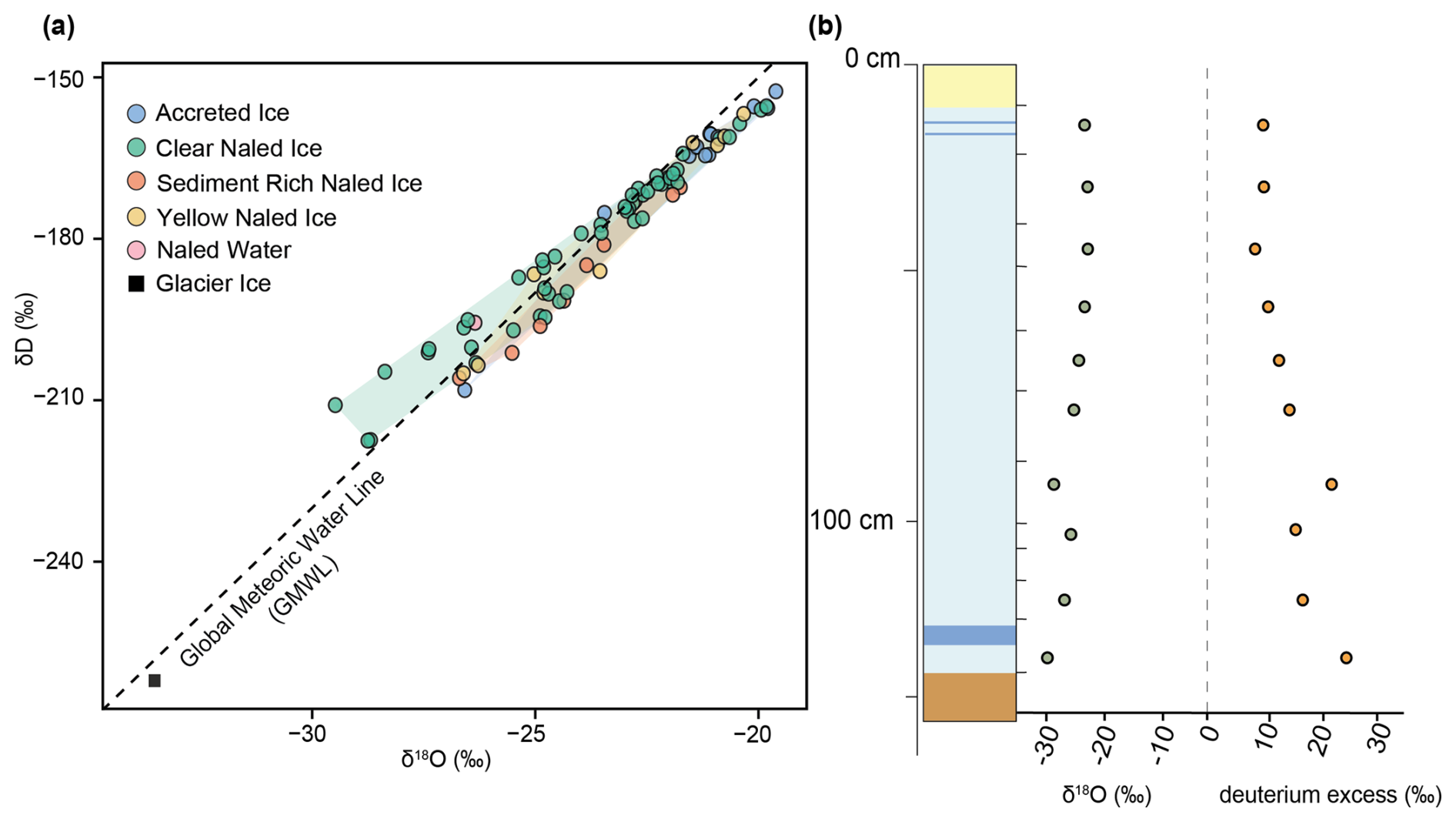
Figure 10 Summary of stable isotope analyses of different ice types. (a) Cross-plot of δD vs. δ¹⁸O compared to the Global Meteoric Water Line (GMWL). (b) Down-core change in δ¹⁸O (green points) and deuterium excess (orange points) in naled core I8. Shaded regions in panels (a)–(c) denote the range of isotope and chemical data for ice and water. Note, only a subset of samples were analysed for stable water isotopes.

Naled cores I1, I7, I8, I11 and I12 were all located in the main proglacial river channel. Naled I1 was located closest to the glacier and extracted from beneath a layer of mud, whereas all other naled icings were collected from clean ice surfaces. All cores sampled from the main channel lack yellow ice layers apart from I8, which had a distinct yellow layer at the very surface and yellow water at the base of the core (Fig. 8). These main channel cores generally exhibit moderate TDS concentrations, except I8, which reaches up to 132 mg L⁻¹ at its base and 3098 mg L⁻¹ in the water. ${\mathrm{HCO}}_{\mathrm{3}}^{-}$ dominance is consistent across all main channel cores, ${\mathrm{SO}}_{\mathrm{4}}^{\mathrm{2}-}$ contributions are relatively low compared to some side channel cores. ${\mathrm{NO}}_{\mathrm{3}}^{-}$ is slightly more elevated in I8 than in the other main channel cores. I12 was sampled as a newly emerging naled with only a thin layer of domed ice extracted after it began forming in the main channel overnight in March 2024. Here, the very surface of the naled ice was sampled and showed moderate TDS concentrations of 24–40 mg L⁻¹ with an almost even proportion of ${\mathrm{HCO}}_{\mathrm{3}}^{-}$and ${\mathrm{SO}}_{\mathrm{4}}^{\mathrm{2}-}$.

Side channel cores, I2, I3, I4, I5, I6, I9 and I10 show greater variability in both TDS concentrations (2–500 mg L⁻¹in ice and 2100 mg L⁻¹in naledwaters) and ion proportions. While ${\mathrm{HCO}}_{\mathrm{3}}^{-}$ and Ca²⁺ dominate, ${\mathrm{SO}}_{\mathrm{4}}^{\mathrm{2}-}$ contributes more proportionally across several cores, most notably the naled water in I2, I6, and I10. Core I10 is particularly distinct, with ${\mathrm{SO}}_{\mathrm{4}}^{\mathrm{2}-}$ comprising over 40 % of total ions throughout and TDS values reaching up to 548 mg L⁻¹ in the yellow ice layers. Naled waters sampled beneath I2 and I3 also show higher TDS concentrations of 2030 and 1032 mg L⁻¹, respectively.

Accreted ice cores (A1–A4) are more uniform in their geochemical signature both within single cores and across cores (Fig. 9c–f). All cores have TDS concentrations between 13 and 39 mg L⁻¹ (Fig. 9c–f). ${\mathrm{HCO}}_{\mathrm{3}}^{-}$ and Ca²⁺ consistently dominate, comprising 50 %–80 % of anion and cation proportions, respectively. The most variability is seen in accreted core A4, where ${\mathrm{SO}}_{\mathrm{4}}^{-}$ dominates the anions in some of the core sections. Accreted cores also have marginally higher proportions of K⁺ compared to the naled ice cores.

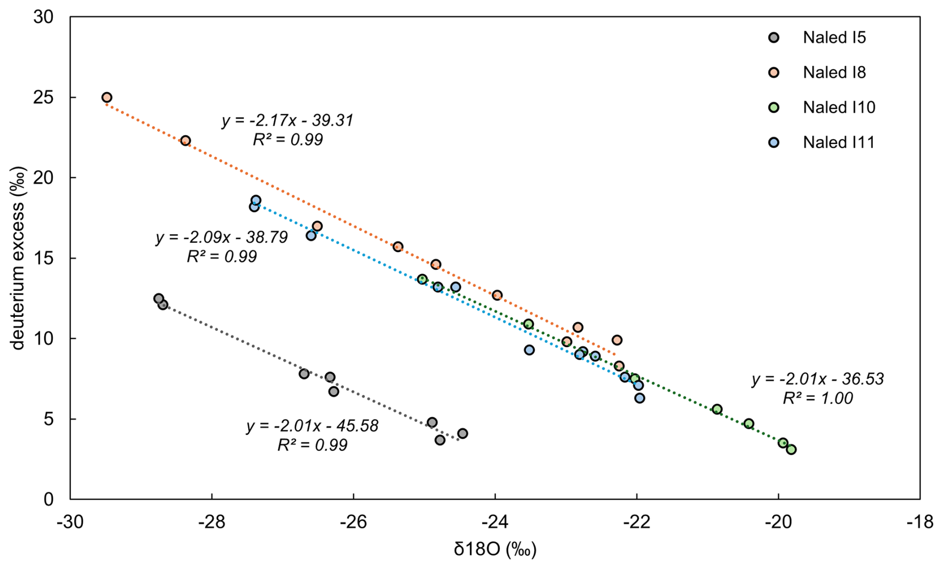
Figure 11 Cross-plot of deuterium excess vs. δ¹⁸O of naled ice samples I5, I8, I10 and I11 on hypothesised freezing curves. All samples plot along the freezing curve with increasing δ¹⁸O and decreasing deuterium excess values with depth, indicative of sequential freezing downcore.

4.4 Stable water isotopes

Isotopic compositions (δ¹⁸O and δD) reveal accreted ice samples have slightly higher δ¹⁸O and δD values (Fig. 10a; −21 ± 1.7 ‰) compared to naled ice (Fig. 10a; −24 ± 2.3 ‰). Surface glacier ice plots separately from all naled samples with the lowest δ¹⁸O value (−33.5 ‰), indicating the naled ice is distinctly different in water source and/or formation mechanism than surface glacier ice (Fig. 10a). Deuterium excess (D-excess = ${\mathit{\delta }}^{\mathrm{2}}\mathrm{H}-\mathrm{8}\cdot {\mathit{\delta }}^{\mathrm{18}}\mathrm{O}$) values range from approximately 3 ‰ to 32 ‰ with a general trend of decreasing deuterium excess with increasing δ¹⁸O values (Fig. 11).

Changed in isotopic composition were also observed down-cores, revealing potential freezing mechanisms. Within naled core I8 (Fig. 10b) δ¹⁸O values generally decrease downcore (the lowest values detected at 132–146 cm of −29.5 ‰) whereas deuterium excess increases from 9.8 ‰ at the top of the core to 25 ‰ at the base due to increasing fractionation processes downcore (Fig. 10b). However, a distinct but slight increase in δ¹⁸O and decrease in deuterium excess was noted at 104–108 cm. When plotted on a freezing curve, naled ice samples I5, I8, I10 and I11 all display R² values of > 0.9, suggesting sequential freezing downcore (Fig. 11). However, some core sections (in I2, I3, I4, I6, I7 and I9) do plot away from the freezing line with R² values of 0.07–0.93 (Fig. S4 in the Supplement). These sections represent discrete intervals of an increase in δ¹⁸O and decrease in deuterium excess (also seen in Fig. 10b), suggesting the start of a new freezing package.

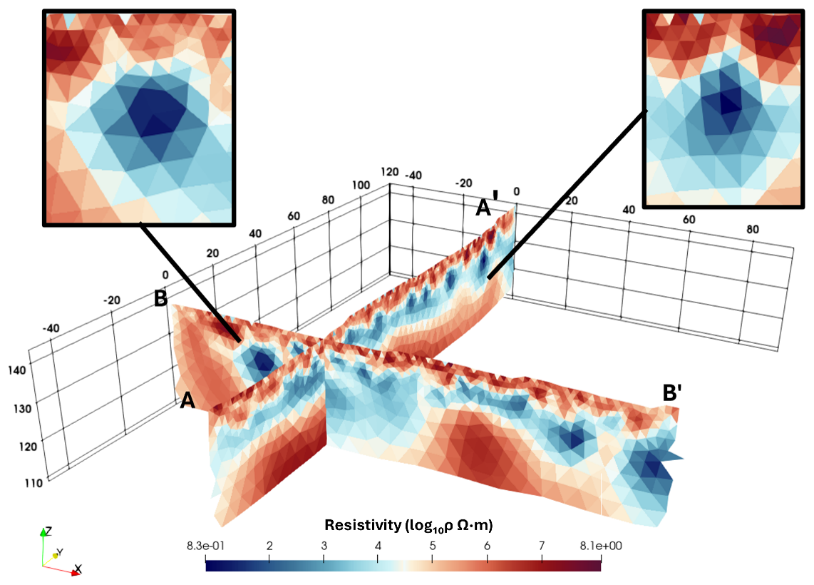
Figure 12 Two intersecting Electrical Resistivity Tomography (ERT) profiles surveyed in front of Isunnguata Sermia (location mapped on Fig. 1). Depth and distance from starting location in metres. Resistivity values span a wide range (from log₁₀ρ ∼ 1 to over 10.8), suggesting significant variations in moisture and/or porosity and/or liquid/frozen contrasts. Pockets of low resistivity, typical of high porosity or water-rich sediment zones, are shown in highlighted boxes.

4.5 Electrical Resistivity Tomography

Electrical Resistivity Tomography (ERT) surveys were conducted < 400 m from the terminus of Isunnguata Sermia, in an area where gravel-rich sediments dominate (Fig. 2). The resulting ERT images (Fig. 12) reveal considerable spatial heterogeneity in subsurface resistivity, spanning from log₁₀ρ ∼ 0.83 to > 8.1. In both ERT profiles, the uppermost layer (∼ 1–5 m below the surface) is dominated by high resistivity values (log₁₀ρ > 10.5), often indicative of dry and (at least partially) frozen material (Kneisel et al., 2014). As the surface is dominated by unsaturated gravel-rich glacial outwash material and compacted till, we expect this uppermost subsurface layer is similar in character.

Beneath the high resistivity layer, an intermediate zone (approximately 5–15 m below ground level) exhibits markedly lower resistivities (log₁₀ρ ∼ 2–4), varying across both profiles (yellow/white/blue colours in Fig. 12a). Bound by higher resistivity above and below, this zone likely represents a saturated sediment layer composed of sands/gravel and/or finer material or fractured bedrock (Palacky, 1987; Hauck and Kneisel, 2008; Reynolds 2011). Each of these materials can host groundwater, ice or subglacial meltwater. Localised zones of even lower resistivity (log₁₀ρ ∼ 1–2) are observed within this intermediate zone in both profiles (Fig. 12a, insets). Their geometry is suggestive of discrete pockets or conduits of moisture, potentially reflecting melting permafrost or glacial outflow pathways (e.g., Hauck and Kneisel, 2008). In both profiles, resistivity values abruptly return to log₁₀ρ ∼ 10.5 and then log₁₀ρ ∼ 10.6 Ωm beneath the intermediate zone. We interpret this to be drier sediments and/or frozen ground/ice (Kneisel et al., 2014), which would be likely in the forefield of Isunnguata Sermia in winter.

5 Discussion

5.1 Naled ice formation mechanisms

Time-lapse camera footage, along with geochemical analyses of naledi and geophysical investigations of the glacial foreland at Isunnguata Sermia have allowed us to capture naledi formation mechanisms in unprecedented detail. Our data show icings forming under both confined and unconfined water input conditions.

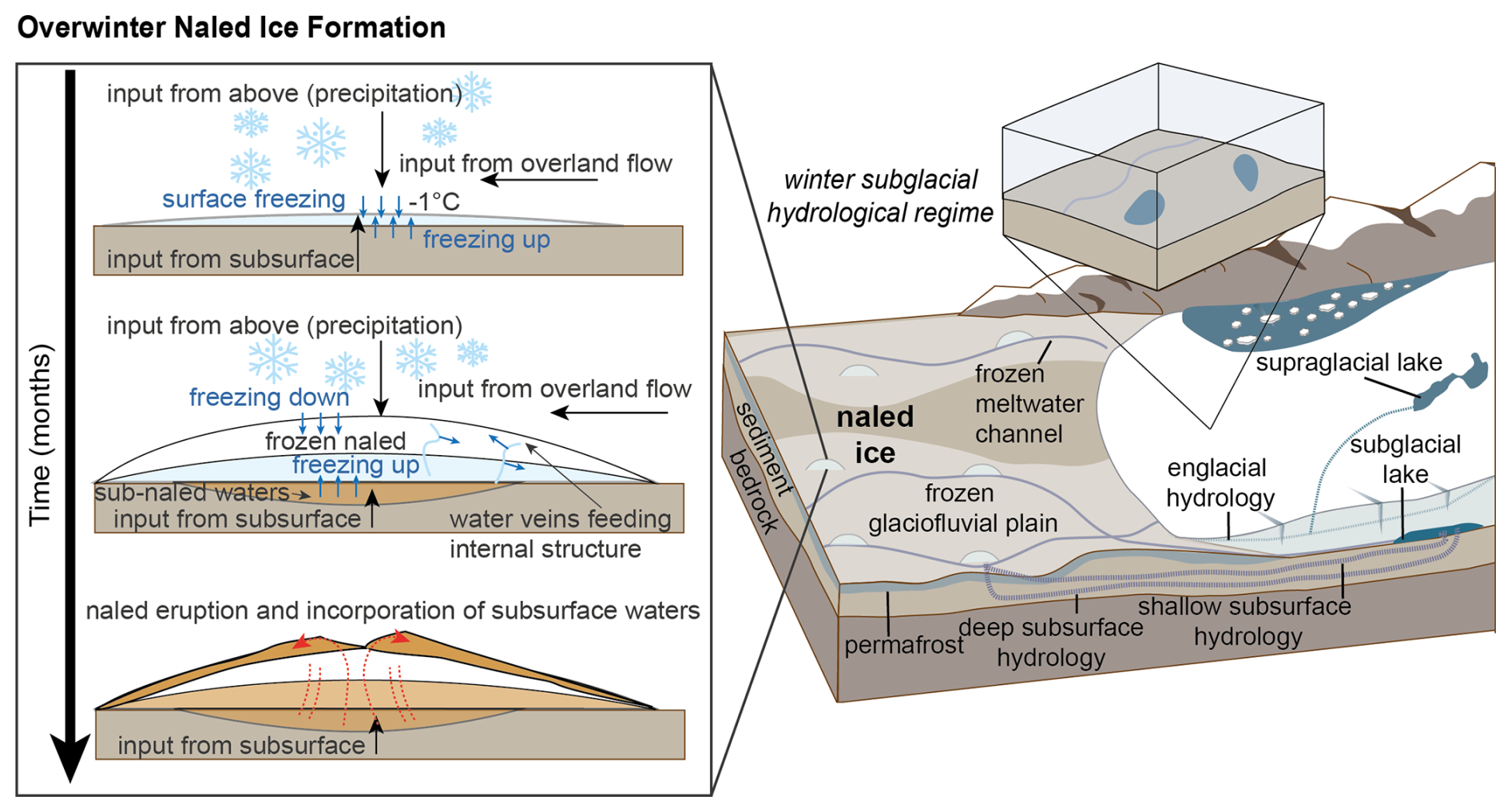
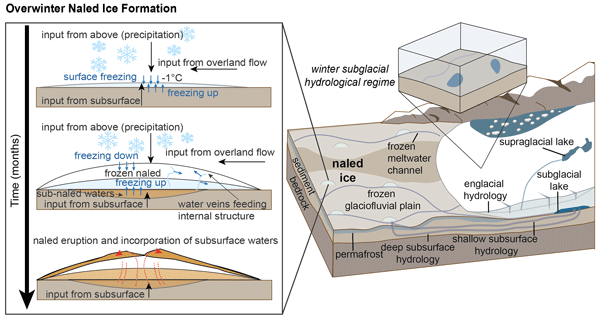
Figure 13 Conceptual diagram of naled ice formation mechanisms in western Greenland, based on ice facies, geochemical evidence and geophysical surveys of the proglacial area in front of Isunnguata Sermia. Inset box shows the evolution of naledi through winter, where water with long subsurface residence times discharges into the proglacial forefield. Other water sources, such as supraglacial and englacial melt, also contribute to naled ice layers. Naledi in this area form from both bottom-up and top-down mechanisms – incorporating two existing theories of naled formation. Water upwellings freeze onto the underside of the naled ice, and overland flow from supraglacial melt, englacial melt and precipitation freeze on top of the ice.

In the confined condition, ice layers build up into dome-like structures, fed by the upwelling of waters from below (Figs. 5 and 13). The waters likely originate from subglacial sources and are transported through subsurface conduits and/or saturated till (Fig. 12). In April 2024, naled ice domes were observed to have started forming overnight suggesting that they may form quickly (Fig. 5e). Following formation of an ice layer that restricts water flow, resultant build-up of water pressure beneath the naled can fracture the ice surface (e.g. Fig. 5c). The method of formation we describe here is akin to the formation mechanism described by Wadham et al. (2000) and Stachnik et al. (2016) (outlined in Fig. 1d–f).

Not all of the naledi studied were exclusively fed from waters below, and our results show that more than one formation mechanism exists with the incorporation of unconfined waters from, for example, englacial flow or precipitation. Automatic camera footage in Fig. 5 demonstrates naledi being built from these unconfined waters, as ice layers accumulate from overland water flow such as supra- and englacial melt and from local precipitation such as the snow event captured in the automatic cameras (Fig. 13). The cameras also captured the incorporation of yellow coloured waters originating off-camera. Due to the colour similarity with the waters collected below naled structures, we believe this overland flow originated from a large upwelling of overwinter waters at a nearby naled location. These camera-derived observations, combined with geochemical analysis, help to explain some of the unique ice facies we observed in the naled ice cores.

The waters with relatively high concentrations of TDS at the base of the naled cores are interpreted to reflect prolonged water storage in the subglacial system (at least over the winter months) - where chemical equilibration and mineral dissolution result in the highest TDS concentrations across our study site (e.g., Gokhman et al., 1987; Hodgkins et al., 2004; Stachnik et al., 2016; Yde et al., 2012). Layers of similar colours and geochemical signatures are also found within the naled cores such as I2, I8 and I10, suggestive of an eruptive process injecting these TDS-rich yellow coloured waters into the ice structure. Our geophysical analysis of the substrate supports these ideas, as low resistivity TMS suggests a saturated sediment layer could be fed by subglacial meltwaters and/or groundwater. The geophysical survey also identifies a potential conduit for water flow (∼ 5 m in diameter), which could efficiently transport subsurface waters over wintertime, contributing to naled ice structures when air temperatures limit overland flow.

The clear naled ice with low solute concentrations suggests waters have had limited mineral surface contact for reactions to occur (such as supra- or englacial melt/storage and/or overwinter precipitation). An alternative explanation is that these layers (most often found at the top of the naled cores) are partially frozen (or partially wasted) ice/slush, which just retains some of the solutes available – as the rest of the solutes have either run off completely (if unconfined), or moved downwards, where they have become concentrated in the bottom layer of the freezing package. For example, in I8 we see very low TDS values (0.8–1.2 mg L⁻¹) in the middle of the core, followed by giher concentrations of 15–141 mg L⁻¹ further down the core, within the most isotopically enriched layers.

The downcore chemical and isotopic variation in naled ice can be explained, at least in part, by freezing processes. During freezing, isotopically enriched water freezes first, with a stronger effect on ²H than ¹⁸O. Remaining, freezing water will fractionate on a freezing slope unlike that of meteoric water, controlled by the initial composition of the water and the fractionation factors of freezing (Jouzel and Souchez, 1982; Souchez and Jouzel, 1984). In a package of ice that froze in a single outburst event, we expect the heaviest isotopes on the top and lighter isotopes downcore. We also expect the concentration of dissolved solutes to significantly increase at the bottom of a freezing package, from the effects of progressive freeze concentration of dissolved solutes in the source water (Halde, 1980).

The stable water isotopes reveal sequential freezing downcore with discrete freezing packages resulting from multiple upwelling events. These upwellings freeze on at the base of existing ice, pushing up into the ice, and creating domed structures over wintertime. However, we also observe that in the top sections of some samples of longer cores (I2 and I7) and the shorter cores below 50 cm (I3, I4, I6 and I9) do not plot on this freezing curve. This indicates a different freezing sequence, potentially forming from a top-down process.

As water discharge is reduced over the winter months, and less glacial sediment is transported, the resulting naled ice is less sediment-laden than summer accreted ice, which forms under faster water flow conditions (Fig. 13). We therefore conclude that the naledi on the forefield of Isunnguata Sermia form through a combination of unconfined and confined water sources, where subsurface waters emerge through the substrate overlain by ice freeze-on below, whereas overland flows and precipitation accumulate from above (Fig. 13).

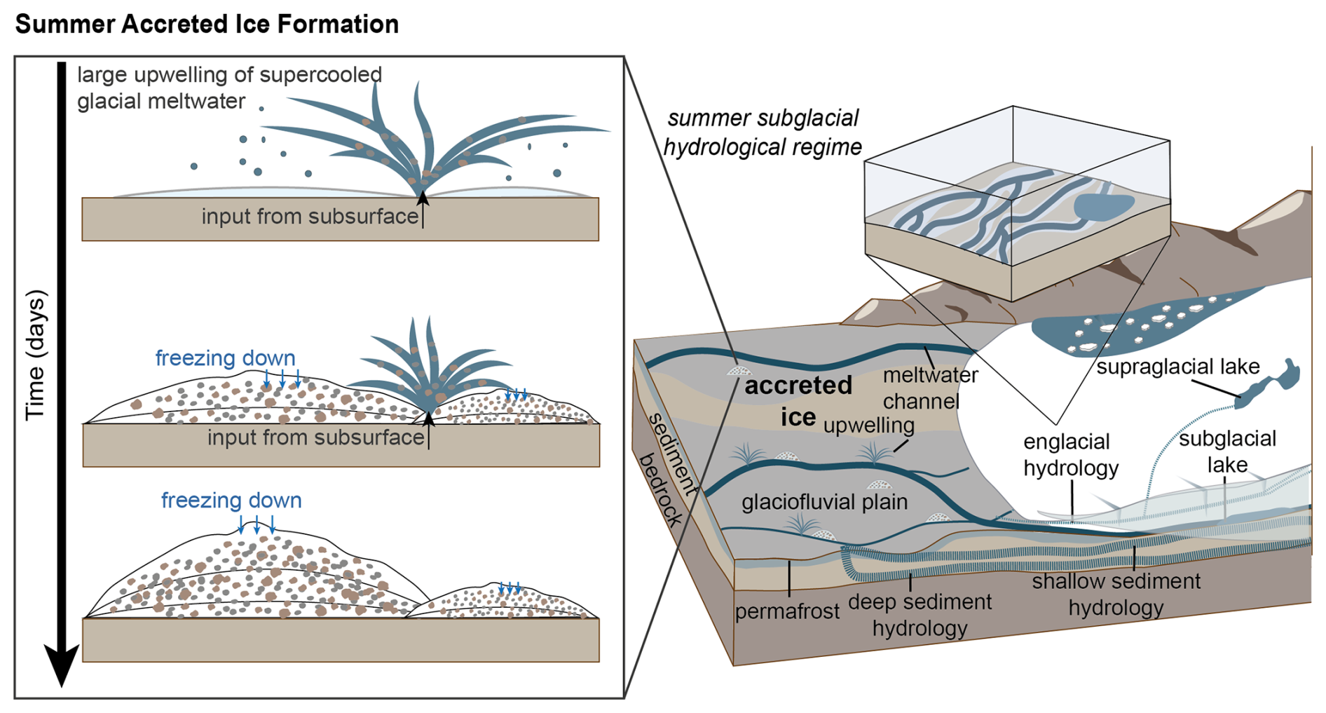
Figure 14 Conceptual diagram of accreted ice formation mechanisms in front of Isunnguata Sermia, Greenland, based on ice facies, geochemical evidence and geophysical surveys of the glacier foreland. Over summer, an efficient subglacial hydrological system moves sediment-loaded waters with low ion concentrations through subsurface hydrological pathways. This allows accreted ice to form where upwellings of highly pressurised supercooled waters erupt into the forefield and freeze adjacent to the upwelling in an isolated event.

5.2 Accreted ice formation mechanisms

The formation of accreted ice was captured on automatic cameras in the late melt season, September–October 2023, after a large upwelling event (Figs. 4 and 6). Based on the speed of their formation and supported by our geochemical analyses, we propose that they form where supercooled meltwater is evacuated into the glacier forefield and quickly freezes creating structures composed of a mix of frazil ice and silt to fine sand sediments (Fig. 14).

The accreted ice samples exhibit a moderately uniform geochemical signature throughout, where the cores are dominated by sediment-rich ice layers. This uniformity between sites and within each core suggests consistent water sources, potentially derived from single or time-constrained outflow events. These cores are also geochemically similar to previously characterised summer outflow waters in other studies (i.e., Graly et al., 2014, 2017). Preserved by cold air temperatures, the ice accretions formed by the late melt season persist through the winter months, although gradual wastage is evidenced by deflation and erosion of the ice surface towards the end of the winter (due to discrete melt events), where melting leaves behind large sediment accumulations. Due to our focus on overwinter ice accumulations, we were not present in the summer months to observe the complete wastage of accreted ice; however, our repeat field campaigns allow us to note that accreted ice structures form in almost the exact same location each year. This observation indicates that the subsurface hydrological system must be stable over interannual timescales.

The subglacial hydrological system in this region drives fast-moving, highly pressurised subglacial waters into the proglacial field, generating large upwellings several metres in height during summer months (Graly et al., 2017). This water is presumably routed through the deep subglacial trough beneath Isunnguata Sermia (Lindbäck et al., 2015), where water will accumulate and interact with sediments and bedrock, before being driven up the reverse bed slope by high water pressure (when the subglacial hydrological system reaches capacity) (Cook et al., 2006; Lindbäck et al., 2014). The subsurface here is likely to be very high-porosity sand/gravel deposited during the Holocene ice margin retreat, which favours “groundwater” flow and not channelised flow. These highly pressurised supercooled waters then freeze into large icing structures close to minimal meltwater output zones at the glacier terminus (Figs. 6 and 14). Currently, the growth and wastage rates of this accreted ice formation are unknown, though we observed that sporadic hours- to days-long upwelling events contribute to the majority of the ice formation (Fig. 6a–c). We hypothesise, based on the results presented here that the formation timescale is likely fast with sudden upwellings of high velocity, highly pressurised waters erupt into the glacial forefield (Fig. 14). Where these structures are formed from single outburst events in the late summer season, they may also incorporate waters from sub-, supra- and ice-marginal lakes where their outbursts are the primary source of the upwelling (e.g., Livingstone et al., 2026).

5.3 Implications and comparisons with existing formation theories

Previous theories of naled formation have adapted either a top-down or bottom-up approach (Fig. 1). One approach details growth from waters below icing structures, with liquid water conduits within naled ice providing transport pathways insulated from the cold surface (Fig. 1f) (Stachnik et al., 2016; Wadham et al., 2000). The other approach describes accumulations from above where the cold, winter air temperature acts as a heat sink, freezing any waters or precipitation that accumulate from above (Fig. 1a–c) (Schohl and Ettema, 1986; Yde et al., 2012). Our observations and results support both of these existing theories. Winter-forming naledi at Isunnguata Sermia form through a combination of top-down and bottom-up freezing processes, whilst summer accreted ice structures form by freeze-on of higher velocity, supercooled waters erupting onto the glacier foreland.

These systems offer insights into hydrological systems in Greenland that are difficult to observe by other means. They also show how water routing can vary spatially and temporally through the melt season. Geochemical differences in ice samples also raise important questions for solute and nutrient release from the Greenland Ice Sheet. With pronounced peaks in TDS detected in the overwinter naled waters, year-round analyses of glacial waters are critical for capturing the full extent of foreland water flow and the impact of these waters on downstream ecosystems, particularly at the release of these solute-rich waters during the initial onset of the melt season. The seasonal changes in geochemistry we observe suggest that solute export in winter may be under-represented in existing literature, which should be considered for a thorough understanding of biogeochemical processes and wider ecosystem effects downstream (Hawkings et al., 2026).

6 Conclusions

Over the course of four field seasons, we have investigated the formation and build-up of winter-forming naledi and summer-forming accreted ice together for the first time, at Isunnguata Sermia, western Greenland. Using 15 ice cores, we geochemically characterised these ice structures for major ion and trace element concentrations, as well as δ²H and δ¹⁸O isotopic composition. By combining geochemistry with geophysical surveys and automatic camera footage, we can fully characterise and interpret icings and the hydrological pathways that drive their formation at Isunnguata Sermia for the first time. The different geochemical signatures and the stratification of ice layers in the naled cores we extracted and analysed suggest that there are multiple water sources and pathways which contribute to naled formation at Isunnguata Sermia. We detected several distinct water types within the naledi, from highly concentrated naled bottom waters enriched in dissolved ions (originating from deep hydrological sources and/or groundwater), through to extremely dilute naled ice layers that most likely originate from supraglacial or englacial waters (which have had limited time and/or opportunity for sediment-water interaction). Our findings demonstrate how naledi can form through a combination of top-down and bottom-up freeze-on processes, where water is supplied from a variety of water sources. We suspect that similar mechanisms will create naledi elsewhere, though one process may dominate over another depending on local conditions (e.g. ice/bed topography, meltwater availability, ground conditions). In contrast, the summer accreted ice is much less geographically diverse, implying supercooled waters from the same (or similar) sources freeze-on quickly, presumably during more discrete, high-output events. By analysing icings year-round, we record a clear hydrological transition at Isunnguata Sermia, between summer (where supercooled waters emerge from efficient channelised drainage systems at pressure) and winter (where more inefficient distributed drainage networks dominate). These seasonal changes drive different geochemical outputs from the Greenland Ice Sheet. Our observations demonstrate the importance of seasonality in solute availability and show the importance of measuring glacier meltwater contributions to proglacial groundwater systems and downstream ecosystems over longer study intervals.