Reconstructing Glacier Dynamics in Complex Terrain with ICESat-2 and Gaussian Process Interpolation

We apply Gaussian Process Regression (GPR) to ICESat-2 along-track height change data to generate spatially continuous glacier height change fields across two glaciated regions with complex topography and dynamic behaviour: Larsen-B (Antarctic Peninsula) and central Southern Svalbard. For Larsen-B, GPR-derived average height change rates from 2021–2024 are −0.61 ± 0.02 m a⁻¹, corresponding to a volume loss of 4.55 ± 0.17 km³ a⁻¹, similar to independent estimates from TanDEM-X. In Svalbard, we observe widespread average thinning (−1.62 ± 0.03 m a⁻¹) and detect clear signals of surging glaciers. GPR's multi-dimensional, uncertainty-aware framework enables accurate interpolation across data gaps and supports the detection of localized dynamic events, such as surges. Sensitivity tests show that interpolation errors increase with gap size, slope, and extrapolation distance. Our findings demonstrate that GPR is well-suited for enhancing the spatial and temporal resolution of altimetry-based glacier monitoring, enabling improved estimates of height and volume change while reconstructing spatially localized phenomena such as surge activity and other transient glacier dynamics.

1 Introduction

Spaceborne altimetry has become a cornerstone in the observation and quantification of ice sheet and glacier volume changes over the past two decades. Satellite altimeters such as ICESat, ICESat-2, and CryoSat-2 have provided valuable long-term records of surface height change, enabling mass balance estimates for both the Greenland and Antarctic Ice Sheets, as well as other glacierized regions worldwide (Gardner et al., 2013; Shepherd et al., 2019; Smith et al., 2020). Laser altimeters, including NASA's ICESat (2003–2009) and its successor ICESat-2 (launched in 2018), offer high vertical accuracy and dense along-track sampling, but require clear-sky conditions (Markus et al., 2017). Conversely, radar altimeters, such as ESA's CryoSat-2, can acquire data in cloudy conditions, but have lower accuracy than laser altimetry due to the complex interaction of the radar with the snow and ice surface and their performance degrades in areas of steep and complex terrain due to issues with waveform interpretation and surface slope effects (McMillan et al., 2014; Nilsson et al., 2022).

ICESat-2 has brought significant improvements in spatial and temporal coverage compared to its predecessor, ICESat. With a continuous orbit repetition rate of 91 d (ICESat operated in a campaign mode) and a six-beam configuration (ICESat only had a single beam), ICESat-2 provides more frequent observations and improved spatial sampling across the cryosphere (Neumann et al., 2019). Despite its precision, ICESat-2 provides height measurements only at discrete points along its ground tracks, like all altimeters. To overcome this sparse sampling, spatial interpolation is needed to generate continuous fields of height change that are essential for applications such as glacier mass balance assessment and data assimilation (Howat et al., 2008; Nilsson et al., 2015, 2022).

A variety of interpolation techniques have been applied to ICESat/ICESat-2 data, including inverse distance weighting (IDW), polynomial surface fitting, and kriging (Fan et al., 2022; Moholdt et al., 2010; Zhang et al., 2012). Kriging, a geostatistical method rooted in Gaussian process theory, has the advantage of providing both predictions and associated uncertainty estimates based on spatial covariance. Other methods, such as IDW or polynomial fitting, generally do not provide uncertainty estimates and may fail to capture the physical drivers of variability in ice surface height change, particularly in regions with sparse or uneven sampling.

Gaussian Process Regression (GPR) is a non-parametric, Bayesian interpolation framework closely related to classical geostatistical kriging, which generalizes it by allowing flexible covariance modeling and multidimensional predictor variables, such as spatial coordinates, elevation, slope, aspect, etc. (Rasmussen and Williams, 2005). In both approaches, the interpolated field is represented as a weighted linear combination of observations, where the weights are derived from an assumed spatial covariance structure. While kriging for geostatistics uses an empirically estimated variogram based on geographic distance, GPR applies a probabilistic framework by interpolating the target variable as a realization of a Gaussian process. This approach assigns a joint multivariate normal distribution to the known observations, whose covariance is prescribed by a user-defined kernel function. These differences lead to several practical distinctions. Classical kriging generally operates in two-dimensional geographic space and requires manual variogram fitting and selection of a specific kriging variant (e.g., ordinary, universal, or co-kriging). Incorporating additional explanatory variables, such as elevation or slope, requires extensions or separate regression steps. In contrast, GPR directly allows multi-dimensional feature spaces, where spatial coordinates and auxiliary terrain or glacier-specific predictors are treated jointly within the same covariance kernel. Consequently, complex terrain dependencies, anisotropy, and non-stationary behaviour can be represented directly through the kernel design. Predictions at unobserved locations correspond to the conditional mean of the posterior distribution, analogously to kriging estimates. However, unlike kriging, kernel hyperparameters are optimized jointly by maximizing the marginal likelihood, thereby avoiding subjective variogram fitting and enabling automatic, data-driven determination.

A key advantage of GPR is the availability of posterior variance estimates, which quantify the expected interpolation uncertainty. GPR yields the full posterior predictive distribution rather than only a point estimate, as compared to other classical interpolation techniques like IDW. Thus, spatially distributed uncertainty estimates are provided that directly quantify the confidence of the interpolation for each location independently, similar to Kriging. This is essential for cryospheric applications where measurement uncertainty and spatial gaps can have large impacts on derived volume change estimates. However, a well-known limitation of GPR is its computational cost, which scales cubically with the number of training points due to matrix inversion, making naive implementations impractical for large datasets. Several approaches have been developed to overcome this, including sparse GPR, point methods, and variational approximations (Quiñonero-Candela and Rasmussen, 2005).

In this study, we explore the application of GPR for interpolating ICESat-2–derived height change data over glacierized terrain in Svalbard and the Antarctic Peninsula. We evaluate its performance under varying spatial data coverage by introducing synthetic data gaps of increasing size and comparing interpolated height change fields to withheld ICESat-2 measurements within these masked regions. In addition to spatial gap-filling, we also apply GPR to ICESat-2 data over different periods – including seasonal, annual, and multi-annual intervals – to test its suitability for generating spatially detailed and temporally dense height change estimates. This allows us to assess the robustness of GPR across both spatial and temporal scales, and to evaluate its advantages and limitations in complex glaciated terrain.

2 Study Site

To assess the performance of GPR for spatial interpolation of ICESat-2 height change data, we selected two glaciated regions with distinct characteristics and known challenges for altimetry: the Larsen-B region on the Antarctic Peninsula and central Svalbard in the Arctic. Both sites are marked by complex topography, heterogeneous glacier dynamics, and temporally variable surface lowering. These conditions make them ideal for testing the ability of GPR to capture height change patterns across different temporal scales and glacier types using ICESat-2 data.

2.1 Larsen-B Region, Antarctic Peninsula

The Larsen-B embayment (Fig. 1a), located on the eastern Antarctic Peninsula, is a key example of rapid cryospheric change following ice shelf collapse. In 2002, the disintegration of the Larsen-B Ice Shelf led to a pronounced acceleration of its tributary glaciers, accompanied by dynamic thinning and retreat (Rignot et al., 2004; Scambos et al., 2004). While the initial speed-up has decreased in recent years, most glaciers continue to flow significantly faster than under pre-collapse conditions (Rott et al., 2020). Following a phase of frontal retreat, many of the glacier termini have advanced in recent years, coinciding with a period of persistent sea ice cover that appears to have temporarily stabilized the glacier fronts. However, the breakup of this sea ice in early 2022 was followed by renewed retreat and dynamic acceleration of several outlet glaciers (Surawy-Stepney et al., 2024). The region's rugged topography and variable glacier behavior present challenges for both radar and laser altimetry. While radar altimeters such as CryoSat-2 struggle with steep slopes and narrow glacier valleys, laser altimeters like ICESat-2 can be affected by cloud cover, leading to spatially and temporally inconsistent coverage.

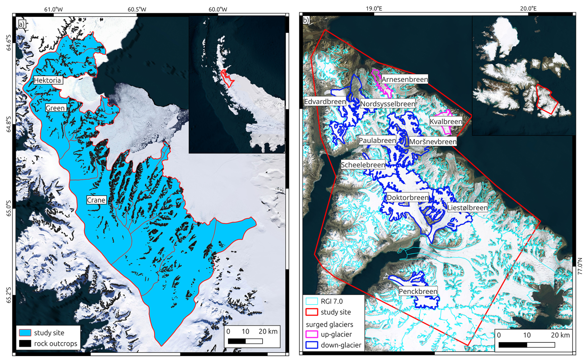
Figure 1 Selected study sites. Panel (a) Glaciers draining in the Larsen-B embayment on the east coast of the Antarctic Peninsula. Glacier outlines and rock outcrop mask from Silva et al. (2020). Panel (b) Subset of Southern Svalbard (called Svalbard in the following). Glacier outlines from the Randolph Glacier Inventory 7.0 (fronts adjusted, see Sect. 3.3), glaciers that surged between 2016 and 2024 according to Mannerfelt et al. (2025) are indicated with blue (down-glacier propagating surge) and magenta (up-glacier propagating surge) outlines. Background: Basemap imagery © Microsoft Bing Maps; data providers include Microsoft and third parties.

2.2 Central Southern Svalbard, Arctic

Central Southern Svalbard encompasses a diverse set of glaciers that vary in size, geometry, and behavior. The selected region (Fig. 1b), called Svalbard in the following, includes both land-terminating and tidewater glaciers, as well as several surge-type glaciers that have experienced surging activity in recent years (Mannerfelt et al., 2025; Sevestre and Benn, 2015). Over the past 30 years, Svalbard has undergone significant glacier mass loss linked to atmospheric warming, increased surface melt, and widespread frontal retreat (Moholdt et al., 2010; Schuler et al., 2020). These changes have led to increasingly negative mass balances and altered the flow dynamics of many glaciers. The terrain in central Svalbard is moderately rugged, with numerous narrow valleys and mountainous areas that pose interpolation challenges for altimetry data. Seasonal snow cover and complex surface conditions add further variability to height change signals.

3 Data

3.1 ICESat-2 Altimeter Data

ICESat-2 is NASA's second-generation Ice, Cloud, and land Elevation Satellite altimetry mission, launched in September 2018. It carries the Advanced Topographic Laser Altimeter System (ATLAS), a photon-counting laser altimeter designed to provide precise height measurements over Earth's cryosphere, oceans, vegetation, and land surfaces. ATLAS emits laser pulses at a wavelength of 532 nm at a repetition rate of 10 kHz (∼ 0.7 m along-track ground spacing between pulses) and operates in a multi-beam configuration with six laser beams arranged in three beam pairs (Markus et al., 2017; Neumann et al., 2019). Each beam has a footprint of approximately 17 m and an across-track spacing of ∼ 90 m between paired beams (center-to-center), and ∼ 3.3 km across-track spacing between beam pairs. This configuration enables ICESat-2 to densely sample Earth's surface with high vertical precision (∼ 2 cm over flat, hard surfaces).

The ICESat-2 project generates several higher-level data products from the raw photon cloud data. The ATL06 product contains geolocated surface heights derived from individual beam pairs, sampled at 20 m along-track intervals by aggregating 40 m segments of raw photon returns. For land ice surfaces, ATL06 includes height, along-track slope, signal quality metrics, and geophysical corrections (e.g., for tides and atmospheric delay) (Smith et al., 2023a).

Building upon ATL06, the ATL11 product (Release 006) provides surface height time series and height change rates at fixed ground reference points along ICESat-2 reference pair tracks. ATL11 is constructed by matching repeat ATL06 observations within an along-track search radius of 60 m and across-track distance of 65 m at the reference points (60 m spacing). A detailed description of the processing can be found in Smith et al. (2023c). ATL11 is specifically produced for regions with significant land ice coverage and where repeat ground tracks exist, which are predominantly at high latitudes (typically above 60° N and below 60° S). However, due to a configuration error at the beginning of the ICESat-2 mission, no repeat ground track measurements were possible for the first two cycles. Thus, we used all available ATL11 data (Smith et al., 2023b) collected between March 2019 and December 2024 to estimate height change rates across our study areas.

3.2 Digital Elevation Models

For topographic reference and surface slope calculations, we utilized high-resolution digital elevation models (DEMs) tailored to each study region. For Svalbard, we employed the 50 m resolution digital terrain model of Svalbard distributed by the Norwegian Polar Institute (NPI). In the Larsen-B region, we used the 12 m refined circum-Antarctic TanDEM-X DEM for the Antarctic Peninsula (Dong et al., 2021). Both DEMs were downsampled, using averaging, to a 200 m grid resolution to match the resolution of our GPR predicted height change dataset (see Sect. 4.1).

3.3 Glacier Outlines

Glacier outlines for Svalbard were taken from the Randolph Glacier Inventory version 7.0 (RGI Consortium, 2023). For the Larsen-B region, we used outlines for 2015 from (Silva et al., 2020), which offer improved delineation of glacier extents on the Antarctic Peninsula. To account for the large frontal area changes in recent years, and to ensure the outlines reflect the most recent terminus positions, the outlines for Larsen-B were further adjusted manually using Sentinel-2 satellite imagery and glacier front positions reported in Surawy-Stepney et al. (2024), and for Svalbard using the calving front positon database from Pyles et al. (2026). This refinement ensured that interpolated height changes were not extrapolated beyond current glacier extents.

4 Methods

4.1 Preprocessing of ICESat-2 Data

We analysed all ICESat-2 ATL11 data (release 006), which contained data through December 2024 at the time of analysis, to derive surface height change rates within the glacier outlines throughout our test sites. The ATL11 h5 files were parsed to extract height above the WGS84 ellipsoid (h_corr), height uncertainty (h_corr_sigma), and time (delta_time) for each Pair Track (pt1, pt2, pt3). Unrealistically high heights (> 2500 m) were excluded. Only points with a fit quality flag of 0, indicating the highest quality of the surface fit used to generate the surface height timeseries for each point from the different cycles, and within the bounds of the glacier outlines were retained.

Height change information was computed for three different time intervals at each study site: (1) long-term trends: To minimize the impact of seasonal variations, surface height changes were computed for measurements with a time separation by multiples of 4 cycles (∼ 1 year). Average rates of height change were derived for Svalbard for the total observation period (March 2019–December 2024, Cycle 3–25). For each ground track point, we obtained a height time series cropped to the earliest and latest valid height measurements. Pairs of observations were selected from each time series based on a preferred separation of 20 repeat cycles (∼ 5 years). However, the frequent cloud cover at both study sites forced us to add a temporal buffer of ± 1 cycle to increase the spatial coverage of height change measurements. Consequently, if no suitable pair was found, pairs within a range of 19 to 21 cycles were also accepted. At Larsen-B, the long-term trends were derived for December 2020–December 2024 (Cycle 10–25), in order to facilitate a direct comparison with the TanDEM-X derived elevation change information (2021–2024, see Sect. 4.3.1). Here, a preferred separation of 12 cycles (∼ 3 years) and a buffer of 11–13 cycles was applied; (2) annual height changes: Subsets from January of the starting year to December of the subsequent year were generated. Pairs of valid height measurements with a preferred separation of 4 cycles and a buffer of ±1 cycle were used to estimate the height change rates; (3) seasonal height changes: To evaluate the applicability of our GPR-based approach on seasonal temporal scales, we additionally tested input datasets that used height differences derived from only a single ICESat-2 repeat cycle (91 d).

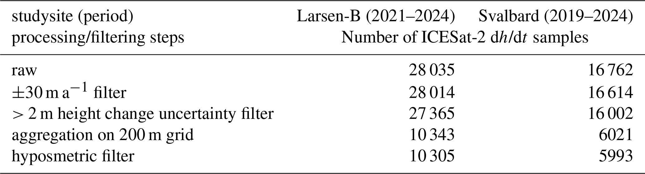
For each dataset, observations with extreme change rates (> ± 30 m a⁻¹ for the long-term and > ± 50 m a⁻¹ for the yearly and seasonal datasets) were removed to reduce outliers. Moreover, each height measurement of the ATL11 data is accompanied by an uncertainty estimate (h_corr_sigma). If the sum of the uncertainty estimates for an observation pair, used to assess the height change for a ground track point, was larger than 2 m, the height-change value was excluded from further analysis. ICESat-2 provides a dense measurement series along the ground tracks. Considering the size of the glaciers in our study areas and to account for computational costs, we selected a 200 m spatial resolution for all further analysis. Height change estimates were spatially down-sampled onto the 200 m Polar Stereographic grid (EPSG 3413 and EPSG3031 for Svalbard and Larsen-B, respectively) using the mean value within each grid cell. Each gridded ICESat-2 height change point was additionally annotated with terrain height and slope of the reference DEM, as well as the corresponding glacier ID.

Our resulting height change data revealed remaining outliers, which affected the GPR output. To further reduce outliers, we implemented an additional filter. We introduced a filter based on the hypsometric distribution of the height change rates at each glacier; height change values were grouped by glacier and binned in 50 m elevation intervals. Within each bin, the median and normalized median absolute deviation (NMAD) were calculated. Outliers were identified per bin as those values exceeding three times the NMAD or having an absolute deviation greater than 5 m a⁻¹. For glaciers with strongly varying height change patterns, the filter also removed a small number of observations tied to the surging process. Overall, the change pattern was not affected, since the filter dismissed only ∼ 0.4 %–0.7 % of all measurements. Moreover, spatially isolated outliers persisted in the upper glacier areas with steep slopes, often near nunataks. These points often represent the only measurements for a specific elevation bin, hampering our filter approach. Since only minor sections of our study areas were affected by the remaining outliers, we decided not to apply any additional filtering to the height change data. The number of samples obtained for the individual processing and filtering steps are summarized in Table 1 for the multi-annual datasets.

Table 1 Number of dh/dt samples obtained from ICESat-2 for the different processing and filtering steps for the multi-annual datasets.

4.2 Interpolation Using Gaussian Process Regression

We applied a Gaussian Process Regression (GPR) modeling approach to interpolate gridded ICESat-2 height change observations across the glacierized region of Svalbard. The analysis was conducted using the Julia programming language (v1.11.1).

For training of our GPR model, we selected predictors of position (x and y in m, in polar stereographic projection), surface elevation derived from the reference DEM, as well as the unique glacier ID obtained from the respective inventories. Height change patterns between neighbouring glaciers can vary strongly, e.g., glacier surge. To account for the individual glacier dynamics and heterogeneous coverage of the glaciers by measurements, the glacier IDs (integer values) were included as a predictor, with a correlation length of 1 in order to minimize cross-correlations between different glaciers. A more detailed discussion of these issues is presented in Sect. 5.2.1. Changes in ice dynamics can drive large changes in surface height, for surge-type and tidewater glaciers (Rankl and Braun, 2016; Seehaus et al., 2015). Thus, ice flow could serve as a predictor. Following the approach of Hurkmans et al. (2014), we also tested glacier surface velocity information as a predictor for the multi-annual datasets. Therefore, we used the average ice flow speeds throughout our observation periods, derived from the ITS_LIVE (Gardner et al., 2025) yearly ice flow composites. Moreover, surface slope information, derived from the reference DEMs, was also tested as a predictor. In order to evaluate the contribution of each predictor (height, glacier IDs, velocity, slope) on the resulting GPR output, we randomly shuffled a specific predictor across all locations on the glaciers and applied the trained GPR model (with all predictors for the ICESat-2 measurements, without shuffling). This approach is similar to the Permutation Feature Importance (PFI) (Breiman, 2001) method used for evaluation machine learning models. The results are exemplarily shown for the region aroung Doktorbreen and Liestølbreen in Svalbard in Fig. 2. Shuffling of the height and glacier ID predictors led to strong noise in the GPR output (Fig. 2a and d). Whereas shuffling the velocity and slope predictors (Fig. 2b and c) had a less pronounced impact on the GPR output. Consequently, the importance of the latter predictors is lower than for surface height and glacier ID information. Additionally, the experiments with different sets of predictors were carried out using artificial data voids of 7000 m radius (see Sect. 4.3.2). The revealed offsets to the actually measured ICESat-2 values showed only small differences for the different predictors sets (mean offsets −0.03 to −0.07 m a⁻¹, standard deviations 1.37 to 1.49 m a⁻¹). Considering the PFI and artificial data voids analyses and the fact that the computational cost of GPR scale cubically (Sect. 1) with the input, we selected surface height and glacier IDs as predictors for further analyses.

Figure 2 Permutation Feature Importance results for the region around Doktorbreen and Liestølbreen for the period 2019–2024. Panel (a) shuffeling the height, (b) slope, (c) velocity, and (d) glacier ID (GID) predictors.

GPR often performs best with standardized inputs (mean of zero and a standard deviation of one). To “flatten” the height change data to have a ∼ 0 mean spatially, we calculated the mean height change within 100 m elevation bins, linearly interpolated to all observed elevations, and then removed the linear fit from the height change data. Similar to the “remove and restore” approach in geodesy (Nilsson et al., 2022), this linear fit will be added back to the output of the GPR model.

We then modelled the spatial distribution of the “flattened” height anomalies using a GPR with a Matérn 5/2 kernel. We selected the Matérn 5/2 kernel because it provides a balance between smoothness and variability, allowing the interpolation to represent spatially coherent but non-smooth elevation-change patterns typical of glacier surfaces. The kernel with Automatic Relevance Determination (ARD) included four input dimensions, allowing different correlation lengths for each dimension (10 000, 10 000, 100, and 1, for x and y coordinates, elevation, and glacier ID, respectively) while accounting for topographic and glaciological context. GP hyperparameters were optimized using maximum likelihood estimation, and a fixed observation noise variance of log(0.24) was used. Different kernels and combinations of kernel functions, as well as correlation lengths, were tested using the multi-year height change information. The correlation lengths for x and y coordinates were initially estimated using a semivariogram and fitting a spherical variogram model to the “flattened” height change data. At both study sites, similar correlation lengths of ∼ 10 km were obtained. We also tested smaller and larger correlation length, as illustrated examplarily for the region around Doktorbreen and Liestølbreen in Svalbard in Fig. 3. A correlation length of 1 km led to rather patchy results (Fig. 3a), whereas larger correlation length led to some spatial leakage of glaciers with pronounced elevation change signal to nearby glaciers, even separated by ice free areas (Fig. 3c). Different kernel functions and combination were also tested (Mater 5/2 ARD, combination of individual Matérn 5/2 ISO kernel in each dimension, combination of Matérn 5/2 ISO and 3rd order Polynomial kernel, 3rd order Polynomial kernel). The output using the different kernel functions is exemplarily shown in Fig. 4. The Matérn 5/2 ARD kernel showed the most meaningful results, since the combination of four individual Matérn 5/2 ISO kernels or Matérn 5/2 ISO and 3rd order Polynomial kernel led, e.g., to spatial leakage of the strong surface lowering in the upper reaches of Liestølbreen to the neighbouring glacier to the South (Dobrowolskibreen). The pure 3rd order Polynomial kernel showed a very blured and averaged output, which is not meaningful at all. The combination of individual kernel functions for each input dimension led to high-frequency noise and discontinuities in the output.

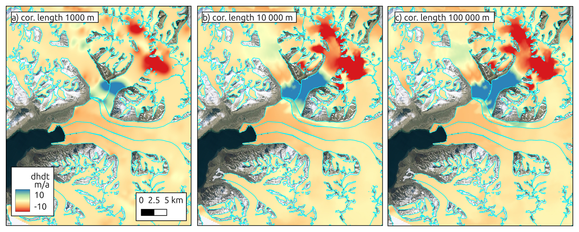
Figure 3 Results for different correlation-length for x and y-coordinates for the region around Doktorbreen and Liestølbreen for the period 2019–2024.

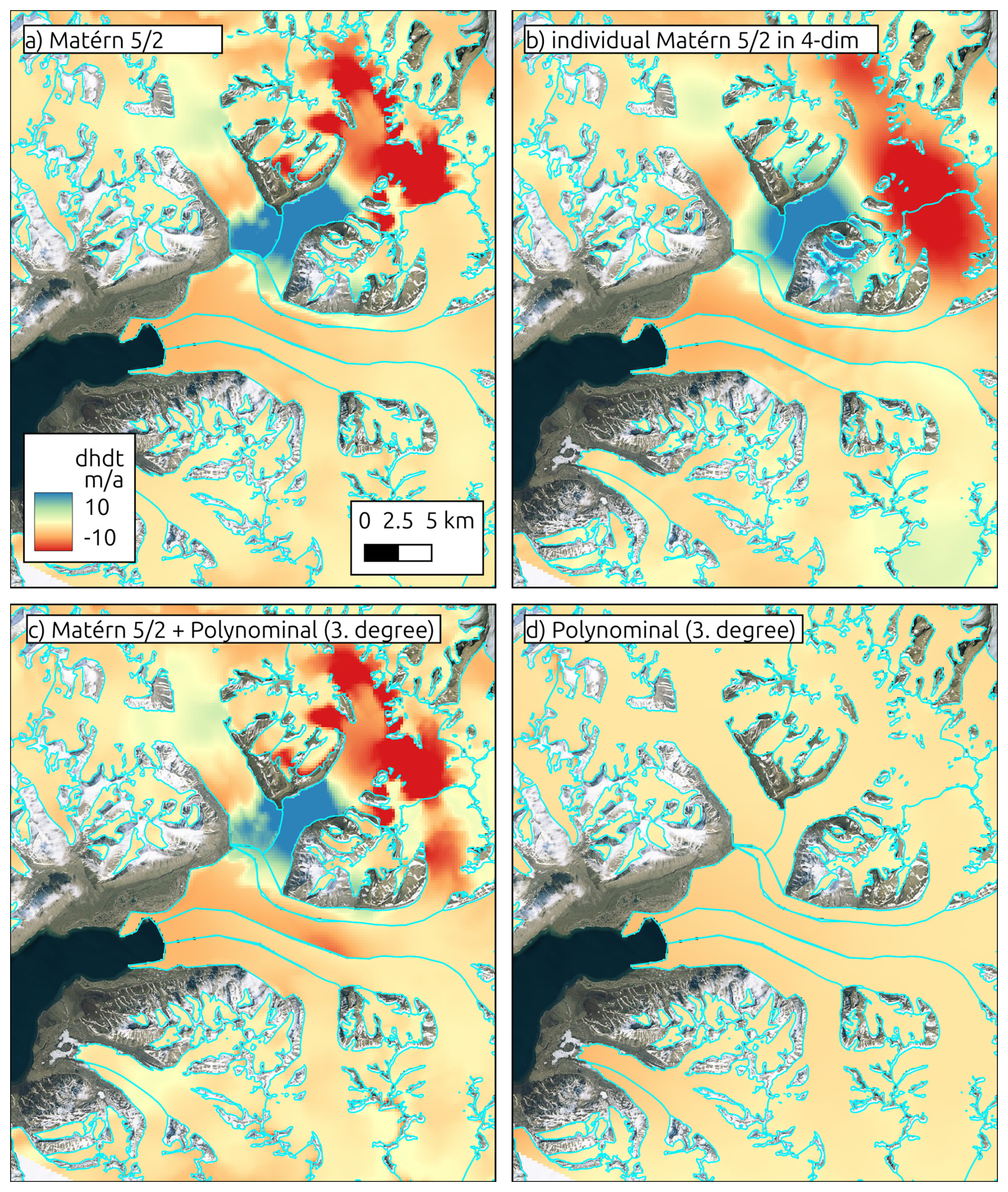
Figure 4 Results for different GPR kernel functions and kernel combinations for the region around Doktorbreen and Liestølbreen for the period 2019–2024.

Consequently, our selected kernel and parameter are suitable for glaciers of 1 km to tens of kilometers in size. However, for smaller mountain glaciers (e.g., like in the Tropical Andes) or large icecaps (e.g., Canadian Arctic), different parameters might be more suitable.

A regular Polar Stereographic grid of prediction points covering the full study area at 200 m resolution was applied. Parallel computing was used to accelerate predictions: the grid was divided into subsets and processed concurrently using Julia's “pmap” function. The GP posterior means were added back to the hypsometric trend to reconstruct the full height change signal. In addition to the elevation-change estimates, the GPR prediction provides a spatially distributed variance field that reflects the modelled uncertainty associated with the interpolation. To obtain a single uncertainty metric σ for each dh/dt map, we averaged the GPR uncertainties σ_GPR (square root of the variance) across all glacierized grid cells and converted this variance into an uncertainty estimate of elevation change following the spatial-correlation scaling proposed by Rolstad et al. (2009):

$$\begin{array}{}\text{(1)}& \begin{array}{lr}\mathit{\sigma }=\sqrt{\frac{A_{\mathrm{cor}}}{\mathrm{5}{A}_{\mathrm{gl}}}}\stackrel{\mathrm{‾}}{{\mathit{\sigma }}_{\mathrm{GPR}}}& A_{\mathrm{gl}}>A_{\mathrm{cor}}\\ \mathit{\sigma }=\stackrel{\mathrm{‾}}{{\mathit{\sigma }}_{\mathrm{GPR}}}& A_{\mathrm{gl}}<A_{\mathrm{cor}}\end{array}\end{array}$$

Where $A_{\mathrm{cor}}=\mathit{\pi }\cdot d_{\mathrm{cor}}$ is the correlation area, A_gl is the analysed glacier area. Specifically, we scaled the mean GPR uncertainty by the effective correlation length (d_cor) of the GPR kernel, yielding an integrated uncertainty that accounts for spatial autocorrelation in both the altimetric input data and the interpolation process. This approach provides a conservative but robust estimate of the total uncertainty of the GPR-derived elevation-change fields and ensures that spatially coherent error structures are not underestimated.

4.3 Quality Assessment

4.3.1 Other Height Change Data

To assess the accuracy of our GPR-based height change estimates, we compared them against independent, spatially continuous surface height change measurements. This was possible at Larsen-B, where acquisitions from TanDEM-X (TDX) for the period 2021–2024 exist. Therefore, TDX Co-registered Single look Slant range Complex (CoSSC) acquisitions from the austral winter 2021 and 2024 were interferometrically processed, co-registered, and mosaicked to obtain DEMs and subsequently a height change field for the study site. We followed the approach described in Seehaus et al. (2023), where a detailed description of the processing is provided.

The TDX height change raster was sampled to match the 200 m grid of the GPR output and cropped to the glacierized areas. An elevation-dependent offset of the TDX measurements was revealed by comparing the TDX and the original ICESat-2 point measurements. This systematic bias is a result of SAR signal penetration difference in the upper firn stratigraphy between the TDX acquisitions and co-registration errors. A linear regression of the TDX anomaly relative to the ICESat-2 was performed to model (n= 10 430) the bias as a function of surface elevation (see Fig. 5). The modelled bias was then removed from the TDX data to obtain a corrected height change map. Subsequently, we computed the difference between the corrected TDX data and both the raw ICESat-2 and the GPR estimates.

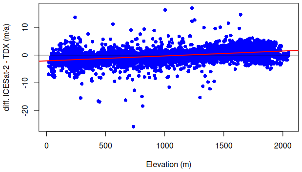
Figure 5 Elevation depended offset between ICESat-2 and TanDEM-X (TDX) elevation change rate measurements at Larsen-B (blue dots) and linear fit (red line) used for correction of the TanDEM-X data due to signal penetration and co-registration errors.

To further evaluate the performance of our GPR–derived elevation-change fields, we compared our multi-annual dh/dt products with the ICESat-2 ATL15 Version 4 gridded surface-elevation-change dataset for the corresponding periods. ATL15 is produced by a least-squares-based algorithm using ATL11 surface height estimates to obtain surface elevation information on various regular grids (1, 10, 20, and 40 km). Considering the topography and glacier geometries at both study sites as well as the resolution of our GPR output, we selected the 1 km grid size ATL15 product and extracted the dh/dt data for the respective long-term observation periods of our study sites (see Sect. 4.1). However, the nominal 1 km grid spacing of ATL15 does not necessarily correspond to an effective spatial resolution of 1 km. ATL15 is generated using a spatially regularized solution to obtain a spatially continuous height-change field from the irregular ICESat-2 sampling. Consequently, where the underlying ICESat-2 observations are sparse, the spatial scale over which information is effectively averaged can exceed the nominal 1 km grid spacing. The effective resolution therefore varies spatially with the density and geometry of the ICESat-2 observations and may be substantially coarser in areas with limited sampling. Please note, that ATL15 coverage is restricted to the Randolph Glacier Inventory glacier outlines in Svalbard, which we also applied for the subsequent comparison with our GPR output.

4.3.2 Artificial Data Gaps

To quantify the sensitivity of the GPR model to data sparsity, we introduced synthetic spatial gaps, similar to other altimetry studies (e.g. Nilsson et al., 2015). We cropped circular gaps of increasing radii (500 m increments, 0–7000 m ∼ 2 times ICESat-2 ground track distance) into the ICESat-2 height change training dataset, in order to simulate data voids due to cloud cover (see Fig. 6). The positions of the gaps were randomly defined using ICESat-2 height change measurement positions, but kept the same for different gap radii. For each gap scenario, GPR was applied to predict the height change fields, and the resulting predictions were compared against the corresponding withheld ICESat-2 height change measurements within the gaps. There is to note that the omission of individual ICESat-2 tracks would cause elongated gaps. Thus, the sensitivity of the GPR model to such gap geometries might be different from that for circular gaps.

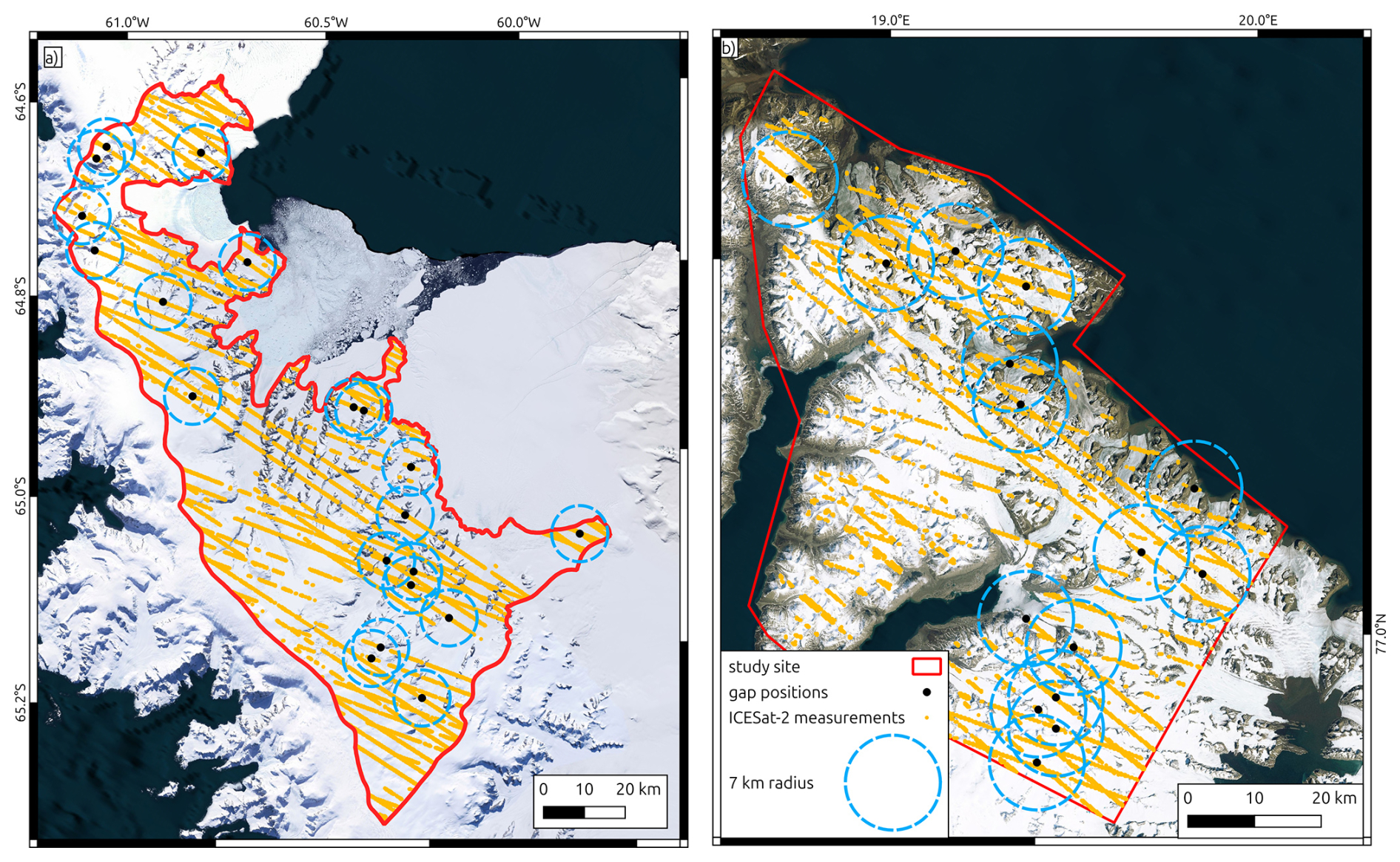
Figure 6 Position of artificial gaps in the ICESat-2 measurements used for sensitivity analysis. Background: Basemap imagery © Microsoft Bing Maps; data providers include Microsoft and third parties.

Summary statistics were computed for each scenario, including mean, median, standard deviation, and NMAD of the residuals. To explore spatial patterns in the prediction errors, residuals were analysed as a function of distance to the nearest ICESat-2 height change measurement, local surface slope (derived from the reference DEMs), and observed height change.

4.3.3 Classical Interpolation Approaches

In addition to the GPR framework, we applied two widely used deterministic interpolation techniques to the ICESat-2 dh/dt measurements in order to benchmark the GPR results. Specifically, IDW and nearest-neighbour interpolation were implemented using the interpIDW and interpNear functions of the terra package in R. Both methods were applied at Larsen-B for the long-term trend dataset, in order to facilitate a comparison to the GPR output as well as to the TDX dataset (Sect. 4.3.1).

Two different search radii for the interpolation were tested. A search radius of 1700 m was selected as a lower bound, corresponding to approximately half the nominal cross-track spacing of ICESat-2 ground tracks (3300 m), thereby allowing interpolation primarily between adjacent tracks. A second, larger radius of 9000 m was used to ensure that all spatial gaps within the study region were filled. The interpolations were performed on the same spatial grid as the GPR to enable a direct comparison of the results.

To further evaluate the ability of the classical interpolation approaches to reproduce original ICESat-2 measurements, we applied both methods to the dataset containing artificial spatial gaps (Sect. 4.3.2). Search radi for the interpolation techniques were 200 m (grid size) larger than the gap radi to obtain sufficient measurements to constrain the interpolation. The interpolated dh/dt values were then compared to the withheld ICESat-2 observations and distances to the next ICESat-2 value.

5 Results and Discussion

5.1 Observed Height Change Patterns

5.1.1 Larsen-B

Using GPR applied to ICESat-2 data, we generated a spatially continuous height change (dh/dt) field for the Larsen-B region over the period 2021–2024 (Fig. 7). The regional average height change is −0.61 ± 0.02 m a⁻¹, with a mean variance of the GPR output of 0.20 m² a⁻², corresponding to a total ice volume loss of approximately 4.55 ± 0.17 km³ a⁻¹ not accounting for sub-aqueous losses for potentially floating glacier sections at the termini. The strongest thinning is observed along the marine-terminating glaciers that previously fed into the collapsed Larsen-B ice shelf, particularly Hektoria, Green, and Crane glaciers, where continued dynamic thinning is evident.

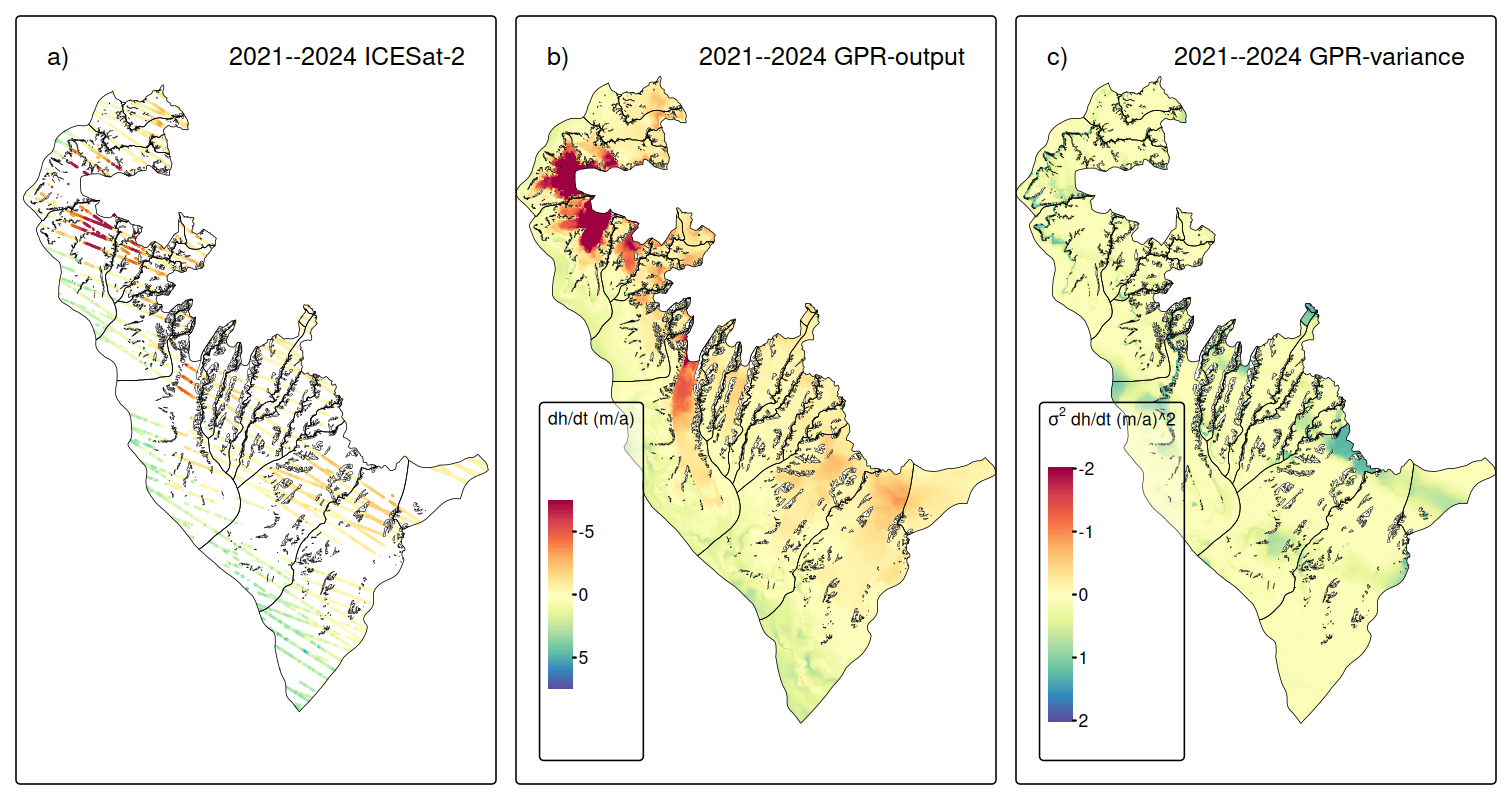
Figure 7 Surface elevation changes at Larsen-B between 2021 and 2024. Panel (a) resampled and filtered ICESat-2 measurements; (b) GPR extrapolated surface elevation changes; (c) Variance of GPR extrapolated surface elevation changes.

When compared with previous studies, our results are consistent with the observed long-term trajectory of glacier evolution in the Larsen-B region. For instance, Berthier et al. (2012) and Scambos et al. (2014) reported strongly increased thinning rates and volume losses in the years immediately following the 2002 ice shelf disintegration, e.g., for our study area, Scambos et al. (2014) observed an ice mass loss of 9.4 Gt a⁻¹ for the period 2003–2008. More recent analyses by Rott et al. (2018, 2020) and Wuite et al. (2015) documented a slowdown in glacier flow and thinning rates (−3.22 ± 0.62 km³ a⁻¹ for 2013–2016), attributed in part to a stabilizing effect by persistent sea ice. Our findings are well below the ice loss rates of the immediate post-collapse years but are elevated relative to 2013–2016 conditions. This increased ice down wasting aligns well with the recent breakup of persistent sea ice in January 2022, as reported by Surawy-Stepney et al. (2024), which had likely helped to stabilize the glacier termini following the collapse of the Larsen-B ice shelf. Following the sea ice breakup, several glaciers – most notably Hektoria, Green, and Crane – showed renewed retreat and acceleration. Ochwat et al. (2024) have also reported enhanced thinning and ice discharge from Larsen-B glaciers in the wake of the 2022 sea ice loss. Our dh/dt maps, long-term and time-series, corroborate these findings of considerable ice volume losses. The time series of yearly dh/dt fields (see Supplement) shows moderate surface lowering rates (∼ 3–5 m a⁻¹) at the tongues of Hektoria and Green glaciers and close to balance conditions for Crane glacier before 2022. However, rapid surface lowering in the range of 15–36 m a⁻¹ at the termini of Hektoria and Green glacier is revealed for the periods 2022–2023 and 2023–2024. At Crane glacier, an increased surface lowering of up to 5 m a⁻¹ is observed only close to the front in 2022–2023, but in the dh/dt field for 2023–2024, an upward expansion and increase of the surface lowering to ∼ 17 m a⁻¹ can be observed. The pattern of lowering suggests dynamic thinning from glacier acceleration. A direct comparison of our findings with Ochwat et al. (2024) is difficult, since they provide height change information for a few specific points and their analysis ends in early 2023. At the lower Green glacier, they reported a thinning of ∼ 11 m between March 2022 and December 2022, which fits our observed dh/dt rates. They also did not observe rapid surface lowering at the Crane glacier in the first year after the sea-ice breakup, except for one sampling point, which was affected by the glacier retreat. The analysis of the speed-up by Surawy-Stepney et al. (2024) indicates that the speed-up at the glacier termini of Hektoria, Green, and Crane glaciers started in mid-2022. It seems that the onset of the dynamic thinning of a Crane glacier was delayed. It is situated in a narrower fjord and has a small calving front compared to Hektoria and Green glaciers. We hypothesize that factors related to the glacier's bedrock geometry led to its delayed response to the sea-ice breakup. This hypothesis might be tested by ice dynamic modelling, where, besides the existing detailed information of ice velocities and calving front positions, a spatio-temporal dataset of dh/dt data, such as presented in this study, could serve for calibration and validation.

5.1.2 Svalbard

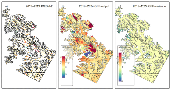
For the Svalbard domain, we observe a considerable mean surface lowering of −1.62 ± 0.03 m a⁻¹, with a mean variance of the GPR output of 0.18 m² a⁻², resulting in an overall ice volume change of −4.85 ± 0.10 km³ a⁻¹. Surface lowering can be attributed to regional atmospheric and oceanic warming (Dahlke et al., 2020; Skogseth et al., 2020). This ice loss trend is about twice as high as the findings by Sochor et al. (2021) and Wang et al. (2022) of −0.80 ± 0.18 and −0.84 ± 0.19 m a⁻¹ for the whole of Southern Svalbard for the period 2003–2019 (ICESat–ICESat-2) and 2019–2021 (ICESat-2), respectively. This general increase in ice down wasting fits with other Svalbard-wide analyses (e.g., Hugonnet et al., 2021; Moholdt et al., 2010; Morris et al., 2020). However, it should be noted that all detected glacier surges in Southern Svalbard by Mannerfelt et al. (2025) are located within our study region. Due to the relocation of ice from higher to lower areas, and the higher ablation rates there (Rankl and Braun, 2016), this explains the considerably higher ice losses as compared to the regional average. Moreover, our revealed uncertainty is about six times lower than the values reported by Sochor et al. (2021) and Wang et al. (2022) for Southern Svalbard.

These surge events are clearly visible in our dh/dt products. At Svalbard, the glacier surges can be classified into two types: down-glacier propagating surges, with a surface bulge moving ice mass from the upper glacier areas towards the lower sections (e.g., Murray et al., 1998), and up-glacier propagating surges, which are initiated by increased ice downwasting at the terminus (e.g., Sevestre et al., 2018). The corresponding surface height changes pattern of both types can be observed in our dh/dt products (see time series of dh/dt for Svalbard provided in the Supplement). Surface lowering in combination with surface height gain towards lower glacier sections is visible at some glaciers, indicating down-glacier propagating surges. Whereas the drastic surface lowering at the terminus with subsequent down wasting at higher regions indicates up-glacier propagating surges.

Mannerfelt et al. (2025) used Sentinel-1 SAR coherence information to identify surging glaciers on Svalbard in the period 2015–2024 (see Fig. 1b). Their findings are consistent with the findings of a global surge-type glacier mapping study by Guillet et al. (2025). Within our study site, both studies identified 10 glaciers that surged within the last 10 years. Three glaciers, Penckbreen, Arensenbreen, Kvalbreen, and Moršnevbreen, started to surge before the start of our observations, according to Mannerfelt et al. (2025). At Moršnevbreen and Penckbreen, only the melting of the downwards shifted ice masses can be observed by our long-term measurements (see Fig. 8), but the yearly dh/dt data (see Supplement) do reveal the increased surface lowering rates in the upper reaches for 2019–2020. At Arensenbreen and Kvalbreen, the surge signal fades out toward 2023 and 2024, respectively. Scheelebreen and Vallåkrabreen started to surge in 2021 and 2023, respectively, and Liestølbreen after 2020, according to Mannerfelt et al. (2025). Using our yearly dh/dt time-series, the onset of the surges at Scheelebreen and Vallåkrabreen can be identified in the dh/dt field from 2019–2020, and is clearly visible in 2020–2021.

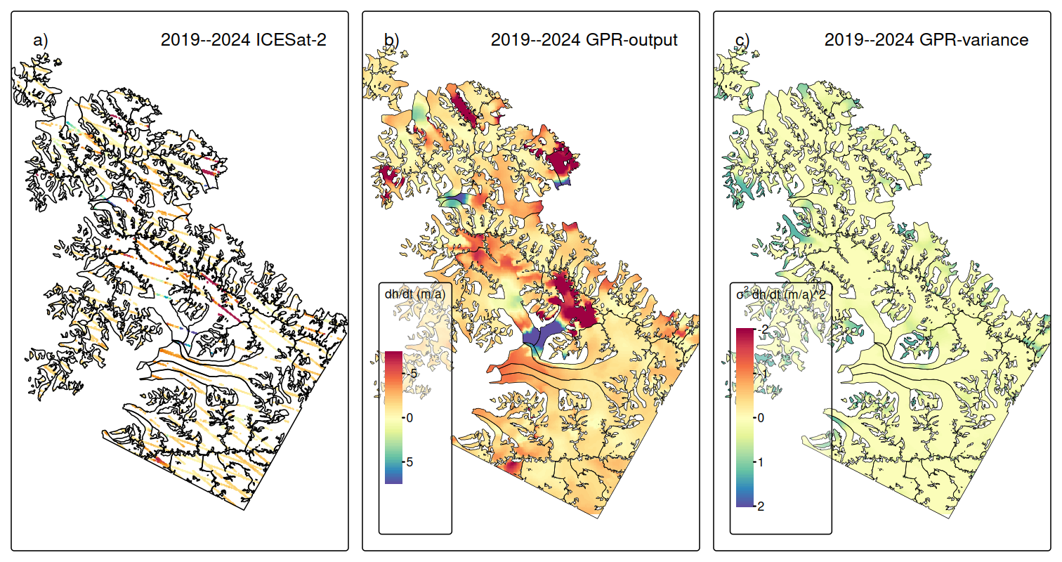
Figure 8 Surface elevation changes at Svalbard between 2019 and 2024. Panel (a) resampled and filtered ICESat-2 measurements; (b) GPR extrapolated surface elevation changes; (c) Variance of GPR extrapolated surface elevation changes.

Mannerfelt et al. (2025) identified already low coherence fronts at both glaciers well before 2021. However, based on their surge start definition (low coherence front reaches the termini for down-propagation surges), their reported values differ from our potential surge starte dates.

Paulabreen, Nordsysselbreen, and Doktorbreen started to surge toward the end of the observation period, according to both studies (after June 2024). However, the onset of mass downwasting can be identified already in the years before from our yearly dh/dt fields (see time series of dh/dt for Svalbard provided in the Supplement). At Nordsysselbreen, increased surface lowering in the upper reaches and uplift at the central part are visible in the dh/dt field from 2022 to 2023. At Doktorbreen and Paulabreen, a similar pattern is found for 2019–2022. The findings by Mannerfelt et al. (2025) suggest that Edvardbreen was close to starting to surge toward the end of their and our study period. However, the dh/dt field from 2023–2024 does not show any signs of surge activity.

In contrast to glacier surface velocity fields, which are already available nearly worldwide on a regular basis (Friedl et al., 2021; Gardner et al., 2025), regular large-scale information on glacier surface height changes is missing. Because of this, Guillet et al. (2025) relied on the Gaussian Process Regression for the temporal extrapolation of the sparse and temporally irregular surface height measurements collected along the center flow lines for their global analysis. Consequently, our approach provides regular elevation measurements throughout the whole glacier area with at least yearly temporal resolution. As discussed above, the initiation of height changes resulting from glacier surge activity can be identified at some glaciers much earlier in our dh/dt product than using the approaches applied by Mannerfelt et al. (2025) or Guillet et al. (2025). However, the start and end definitions of a surge are not clearly defined and differs by each method applied, as also outlined by Mannerfelt et al. (2025). Consequently, our dh/dt product may lead to improved surge detection, process understanding, and early warning systems, which are of interest for natural hazard management, e.g., in High Mountain Asia, where glacier surges have caused flooding events (e.g., Lovell and Muhammad, 2025). We tested higher temporal resolutions down to one ICESat-2 cycle (91 d, see Supplement), but the spatial coverage of ICESat-2 data was determined to be insufficient due to the regular cloud cover at both study sites. We are optimistic that meaningful results at a temporal resolution of a quarter of a year (∼ 1 ICESat-2 cycle) are likely possible at study sites with less frequent cloud cover.

5.2 Quality Assessment

5.2.1 Spatial Leakage

To limit interpolation across dynamically unrelated glacier systems, we incorporated the glacier IDs as a predictor in the GPR model. This addition aimed to constrain spatial predictions within glacier-specific domains and reduce spatial leakage, where surface height change signals from one glacier propagate into adjacent basins. For example, the surges of Arnesenbreen and Mor$\stackrel{\mathrm{ˇ}}{s}$nevbreen led to strong dh/dt signals in the ICESat-2 measurements for the period 2019–2020 (Fig. 9a). Applying GPR interpolation without incorporating the glacier IDs as a predictor (Fig. 9b), the strong surface elevation increase in the lower section of Arnesenbreen leaked to parts of both neighbouring glaciers, where no ICESat-2 data were close by. The glacier tongues are separated by mountain ridges and are dynamically independent. Consequently, the interpolation obtained by accounting for different glacier IDs (Fig. 9c) shows a more meaningful elevation change pattern at the neighbouring glaciers. A similar effect is observed for the strong surface-lowering signal in the upper areas of Moršnevbreen obtained by the ICESat-2 samples, but not for the neighbouring glaciers. Thus, including glacier IDs significantly reduced unrealistic cross-glacier influence, particularly in highly dynamic regions like glacier surges.

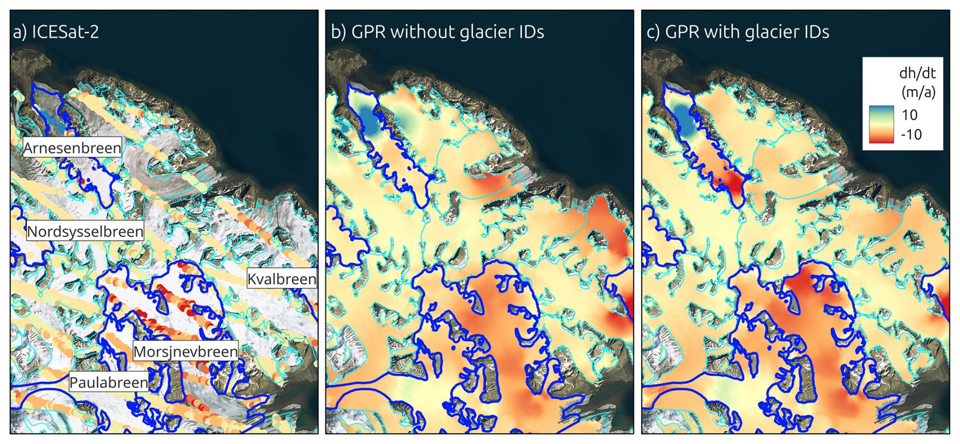
Figure 9 Subset of the Svalbard study site (Fig. 1). Panel (a) ICESat-2 dh/dt measurements for the period 2019–2020, panel (b) GPR interpolation without incorporating glacier IDs as predictor, panel (c) GPR interpolation without incorporating glacier IDs as predictor. Background: Basemap imagery © Microsoft Bing Maps; data providers include Microsoft and third parties.

However, some residual leakage effects remained. In northeastern Svalbard, for example, the surge of Kvalbreen produced strong positive dh/dt signals that extended across the fjord to the glacier south of Moršnevbreen, resulting in apparent slight thickening at the termini, where ICESat-2 data was absent (Fig. 8). Similarly, in the Larsen-B region, a small outlet glacier in the Crane catchment, north of the main terminus, exhibited strong negative dh/dt values that appear to reflect the influence of the main glacier tongue's pronounced thinning (Fig. 7). These instances illustrate the challenge of interpolating in heterogeneous glaciated terrain, especially where dynamic processes vary over short spatial scales and observational constraints are sparse. While the inclusion of glacier ID mitigates such effects, it does not fully resolve them.

5.2.2 Short-term dh/dt Fields and Time Series Performance

When surface height change was estimated using only single-cycle (91 d) ICESat-2 data, spatial coverage proved highly fragmented and sparse, most likely due to persistent cloud cover. The resulting dh/dt fields were often noisy or biased, with localized over- or under-estimations due to limited observational constraints. However, when the absolute height change (dh) since the start of the observation period was reconstructed by integrating the series of GPR-predicted 91 d outputs, a clear and physically consistent pattern emerged. In particular, the evolution of glacier surges on Svalbard – including initiation, peak thickening, and subsequent thinning – was clearly captured by the GPR time-series. This suggests that while single-cycle dh/dt estimates are unreliable on their own, stacking or integrating multiple cycles can reveal meaningful trends and dynamic events. The full-time series figures and animated GIFs illustrating these developments are provided in the Supplement.

5.2.3 TDX Comparison

To assess the validity of our extrapolation approach, we compared our ICESat-2-derived dh/dt field to an independently produced TanDEM-X height change dataset covering 95 % of the ICESat-2 study area for the same period (2021–2024). The spatial pattern of surface height change shows in general consistency between the datasets, with TanDEM-X indicating a mean height change of −0.72 ± 0.01 m a⁻¹ and a total volume change of −5.26 ± 0.07 km³ a⁻¹. The TanDEM-X height change uncertainty is derived based on measurements on stable ice-free areas and considering spatial autocorrelation (see Seehaus et al., 2023), and is about half of the uncertainty obtained for the GPR interpolation results. The mean offset between the two datasets in the overlap region is 0.09 m a⁻¹ for dh/dt and 0.68 km³ a⁻¹ for dV/dt. The dh/dt offsets between the TanDEM-X and ICESat-2 measurements and to the GPR output are illustrated in Fig. 10. Both offset fields show similar patterns, with a clear positive offset in the southern section, indicating that the average offsets between TanDEM-X and the GPR output can be partly attributed to existing offsets between TanDEM-X and ICESat-2 point measurements in this region, which consequently repeat in the GPR output fields, contributing to an overall mean offset of dh/dt by ∼ 15 %. We assume that these offsets are caused by still remaining SAR penetration depth issues in the high-altitude accumulation areas, as well as slight temporal offsets.

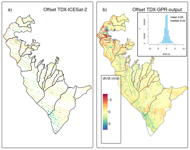
Figure 10 Comparison of ICESat-2 derived height changes with TanDEM-X measurements for 2021–2024. Panel (a) Offsets between resampled and filtered ICESat-2 measurements and TanDEM-X; (b) Offsets between GPR extrapolated ICESat-2 measurements and TanDEM-X (Inset: Histogram of offsets).

Strongest offsets are found at Hektoria and Green glaciers for the GPR output. As mentioned above, these glaciers are undergoing strong and rapid dynamic changes. The spatial extrapolation of ICESat-2 data does not capture all details, leading to these pronounced local offsets.

The wide correspondence between the TanDEM-X and extrapolated ICESat-2 data supports the robustness of our GPR-derived extrapolation method. It confirms the capability of GPR to interpolate altimetry point measurements in complex terrain and dynamic glacier systems.

5.2.4 ATL15 Comparison

Figure 11 illustrates the long-term elevation change rates using ATL15 and the difference between our GPR-derived fields (resampled to 1 km resolution) at both study sites. Across both study regions, the spatial coverage of ATL15 data is substantially more limited than that of the GPR output. In Svalbard, the ATL15 captures the very broad regional distribution of elevation change but provides only partial or no coverage for many of the small, narrow, and steep outlet glaciers. It generally resolves only large-scale dh/dt patterns at Svalbard. Small-scale features, including the narrow dynamic tongues and surge-related elevation-change structures, besides the surges of the large glaciers Doktorbreen and Liestølbreen, that are clearly captured by the GPR fields in Svalbard, are not reproduced in ATL15 and offsets peak at > 10 m a⁻¹. However, the regional mean offset accounts for only 0.13 m a⁻¹ but with a standard deviation of 2.39 m a⁻¹.

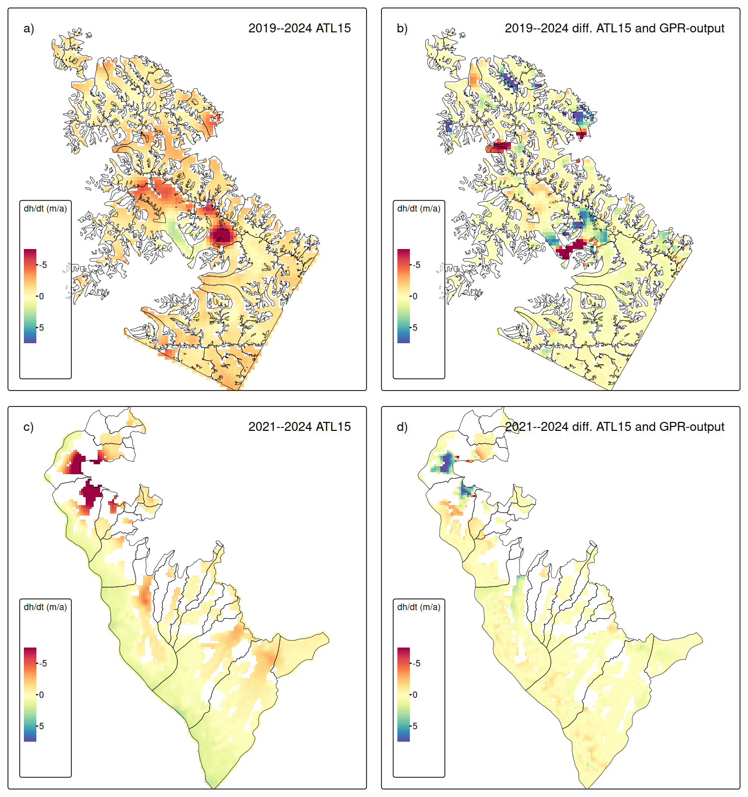
Figure 11 Panels (a) and (c). Surface elevation change rates derived from ICESat-2 ATL15 data product at 1 km spatial resolution. Panels (b) and (d). Difference between the ATL15 rates and GPR-output for the same observation periods for Svalbard (upper panels) and Larsen-B (lower panels).

At Larsen-B, the coverage is even more limited. Only the wide and relatively flat plateau and the wider sections of the outlet glaciers contain valid ATL15 measurements, whereas some of the narrower outlets and steeper valley sections are largely absent from the dataset. A broad thinning across the lower sections of Hektoria, Green, Evans, and Crane glaciers is also revealed by the ATL15 dataset, but the magnitude is in general lower, partially by more than 5 m a⁻¹, as for the GPR output. However, the region-wide mean offset 0.09 m a⁻¹ (standard deviation of 1.07 m a⁻¹) is as low as for the Svalbard test site.

ATL15 total volume change estimates amount to −4.57 and −3.34 km³ a⁻¹ for Svalbard and Larsen-B, respectively. Compared with the GPR-derived estimates (Sect. 5.1), ATL15 captures 94 % of the GPR-derived volume loss at Svalbard and 73 % at Larsen-B. The larger underestimation at Larsen-B may partly reflect the lower magnitude of the average elevation-change signal, combined with the spatial regularization and coarser effective resolution of ATL15, which smoothed out the strong thinning at the termini of Hektoria, Green, Evans, and Crane glaciers. This is also evident in the difference maps between ATL15 and our GPR fields (Fig. 11). In regions of strong dynamic thinning or thickening, ATL15 systematically underestimates the magnitude of elevation change. This is especially apparent at the rapidly retreating glacier tongues at Larsen-B and surge-affected basins at Svalbard, where ATL15 tends to dampen the true signal. These systematic underestimations are most pronounced where the absolute magnitude of dh/dt exceeds several meters per year. We attribute this to the applied spatial smoothing when generating the ATL15 product and coarse effective spatial resolution in regions with sparse ICESat-2 sampling. Conversely, in regions characterized by gentle slopes and modest elevation-change rates – such as the broad plateau surfaces of Larsen-B or the large, slow-flowing glaciers in central Svalbard – the agreement between ATL15 and the GPR output is good, with average offsets < 1 m a⁻¹. Here, both methods converge on nearly identical patterns, suggesting that the GPR model does not introduce artificial structure in areas where the true elevation-change signal is small and spatially coherent.

5.2.5 Artificial Gaps

To assess the robustness of the GPR extrapolated ICESat-2 surface height change rates, we conducted a sensitivity analysis by introducing artificial data gaps.

For Larsen-B, the results indicate a generally low sensitivity of the interpolated dh/dt values to the size of missing data regions (Fig. 12). The mean offset across gap sizes remains close to zero, with values ranging from −0.12 to +0.04 m a⁻¹ with standard deviations of residuals consistently below 0.7 m a⁻¹. Moreover, the mean offsets obtained from the artificial-gap experiments are smaller at Larsen-B than the mean variances of the GPR output (see Sect. 5.1.1). This behavior suggests that the larger spatial variability of the dh/dt field in Larsen-B is well captured by the GPR kernel, that regional glacier change patterns are sufficiently represented in the ICESat-2 point data to allow robust interpolation even across multi-kilometer gaps, and that the interpolation error introduced by artificial data gaps does not exceed the general modelled predictive uncertainty.

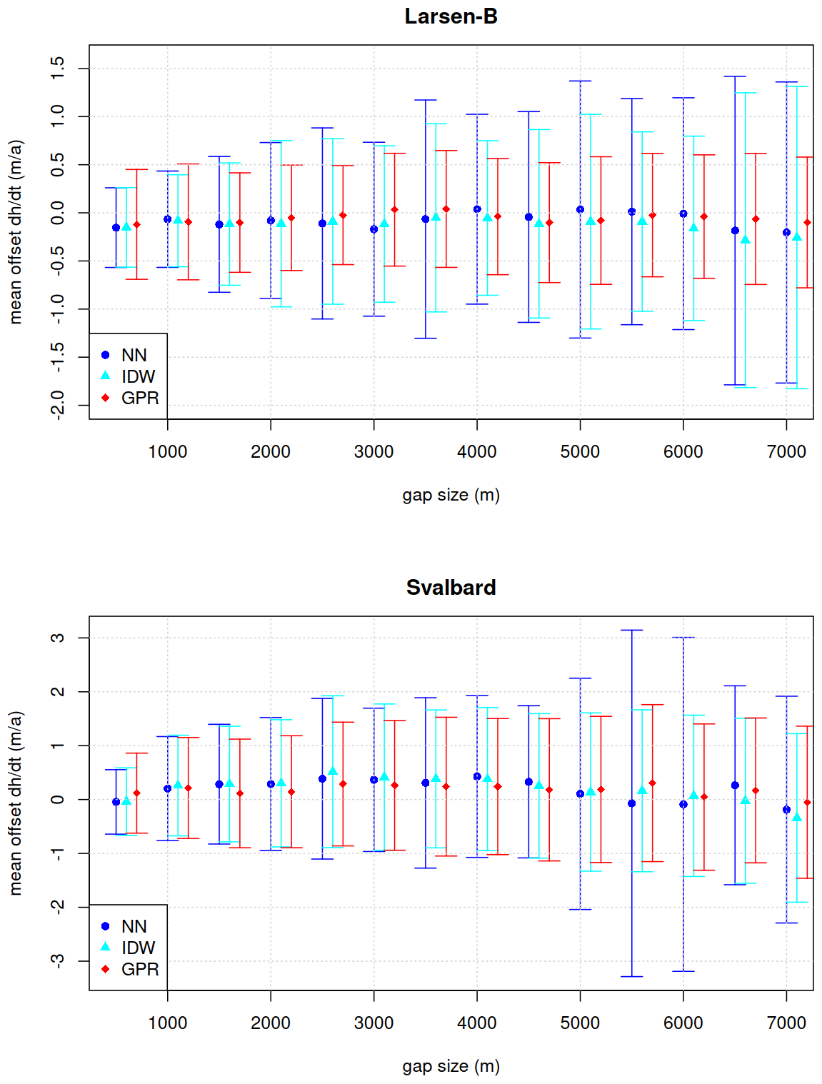
Figure 12 Mean offset between GPR, IDW and Nearest Neighbour extrapolated surface height changes and ICESat-2 measurements for different gap radii. Error bars indicate standard deviations.

In contrast, results for Svalbard show increased sensitivity to gap size (Fig. 12). While the mean offset remains relatively low and varies around zero between −0.05 and 0.30 m a⁻¹, the standard deviation of the offsets increases gradually with gap size, indicating an overall spread of residuals, particularly beyond radii of 3000 m. This pattern reflects the more heterogeneous nature of glacier changes in Svalbard, which include different glacier geometries, small-scale variability from surging glaciers, steep topographic relief, and complex mass balance regimes. Accordingly, the extrapolation of dh/dt fields in such terrain becomes increasingly uncertain with growing data gaps, emphasizing the need for dense altimetric datasets in these regions.

To further evaluate the drivers of interpolation uncertainty in regions with sparse ICESat-2 data, we analyzed how the dh/dt offsets associated with artificial 7000 m data gaps vary with dh/dt and slope. Plots for other gap sizes can be found in the Supplement. Figure 13 shows the relationship between the interpolation offset and the reference (i.e., ICESat-2 observed) GPR derived dh/dt values. A clear pattern emerges in which larger offsets tend to occur in areas with more extreme dh/dt values at both study sites. This trend is not visible for the highest dh/dt bins, where the number of samples is low and statistical noise is high. These results suggest that strong glacier change signals are more difficult to interpolate accurately over large gaps, likely due to their localized nature, which cannot be fully captured by the used spatial covariance structure of the applied GPR kernel.

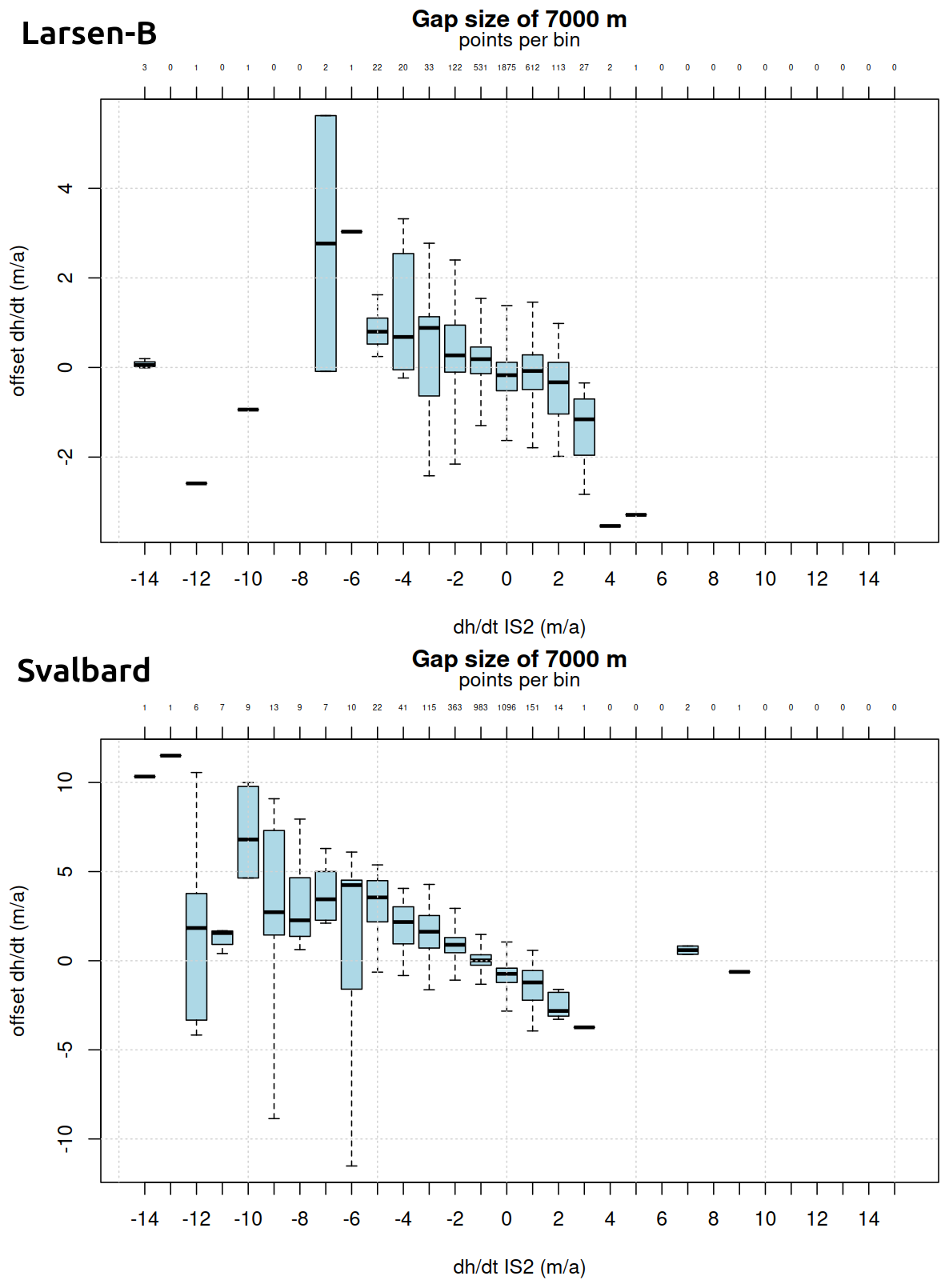
Figure 13 Offset between GPR extrapolated surface height changes and masked ICESat-2 measurements for different surface height change rates, measured by ICESat-2, within the gaps for a gap radius of 7000 m. Whiskers indicate two times the inter-quartile range.

Figure 14 illustrates the dependence of dh/dt error on local surface slope. No clear trend is found for the offsets at Larsen-B. A slight but systematic bias toward more negative offsets is observed as surface slope increases, as found for Svalbard. This trend implies that in steeper terrain, the GPR method may tend to slightly underestimate dh/dt, which could stem from the limited ability of the spatial kernel to account for sharp elevation gradients or the influence of terrain-induced altimetric errors. The results are consistent with previous findings that interpolation in high-relief glacier areas often introduces additional uncertainty (Strößenreuther et al., 2020).

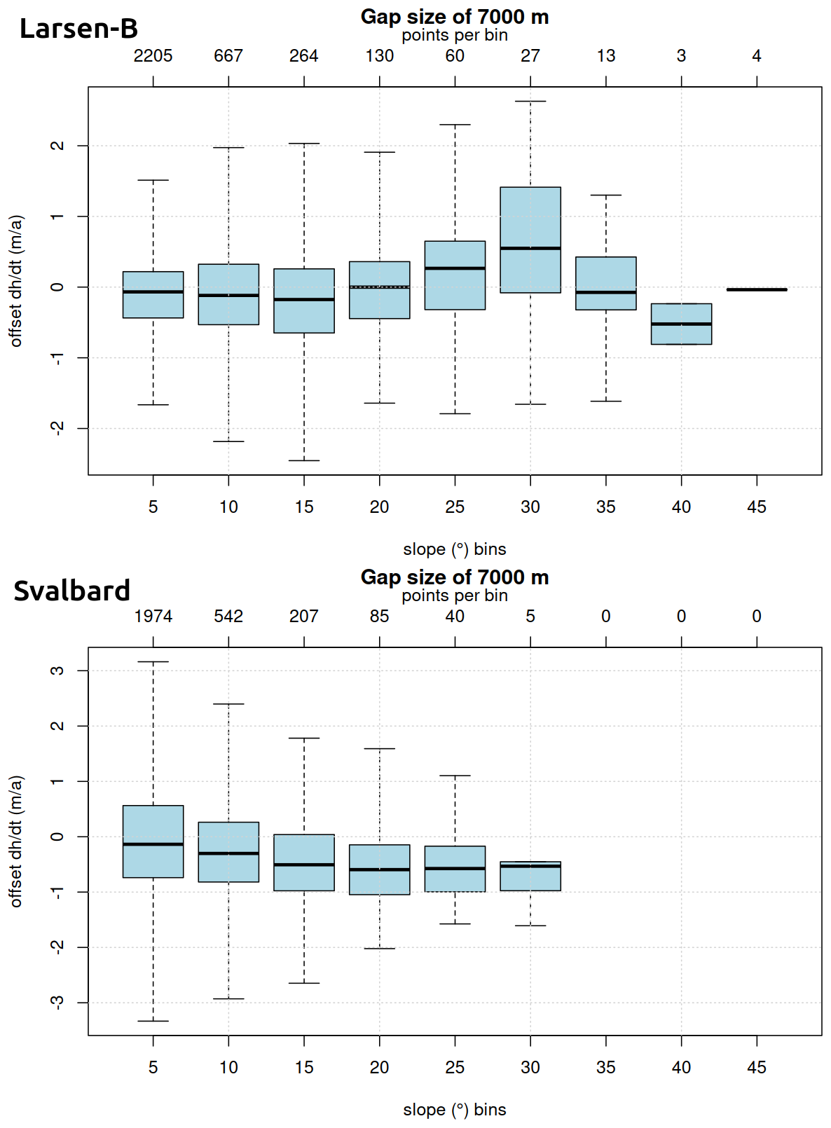
Figure 14 Offset between GPR extrapolated surface height changes and masked ICESat-2 measurements for different surface slopes within the gaps for a gap radius of 7000 m. Whiskers indicate two times the inter-quartile range.

Figure 15 examines the offsets as a function of distance to the nearest ICESat-2 measurement. At Larsen-B, a trend towards negative offsets is found for mid-range distances (5000–7500 m) and positive offsets for larger distances (7500–10 000 m). For Svalbard, a weak but consistent tendency for interpolation to produce more negative dh/dt estimates as the distance to the nearest observation increases is revealed. These patterns align with expectations from spatial statistics, where prediction uncertainty and potential bias grow with extrapolation distance (e.g., Holzenkamp et al., 2025). It reinforces the importance of data proximity in achieving accurate height change estimates, particularly when using nonparametric spatial methods like GPR.

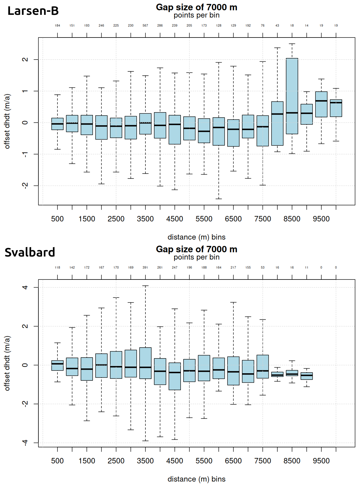
Figure 15 Offset between GPR extrapolated surface height changes and masked ICESat-2 measurements within the gaps for different distances to nearest ICESat-2 measurements for a gap radius of 7000 m. Whiskers indicate two times the inter-quartile range.

5.2.6 Classical Interpolation Comparison

The resulting dh/dt fields of the classical interpolation experiments are shown in Fig. 16. For the smaller search radius of 1700 m, both nearest-neighbour and IDW interpolation reproduce the broad-scale spatial patterns of elevation change by filling the voids between adjacent ICESat-2 tracks. However, large voids remain in areas where the ICESat-2 measurements were hampered by, e.g., persistent cloud cover. The resulting dh/dt fields and differences to the GPR and TDX fields exhibit pronounced local artifacts, including striping aligned with ICESat-2 ground tracks. These effects are most evident in dynamically active regions, in particular at Hektoria, Green, Evans, and Crane glaciers, where elevation change gradients are strong and spatially heterogeneous. For the nearest-neighbour approach, unrealistic abrupt signal changes in along and across the ICESat-2 ground track direction are revealed as well.

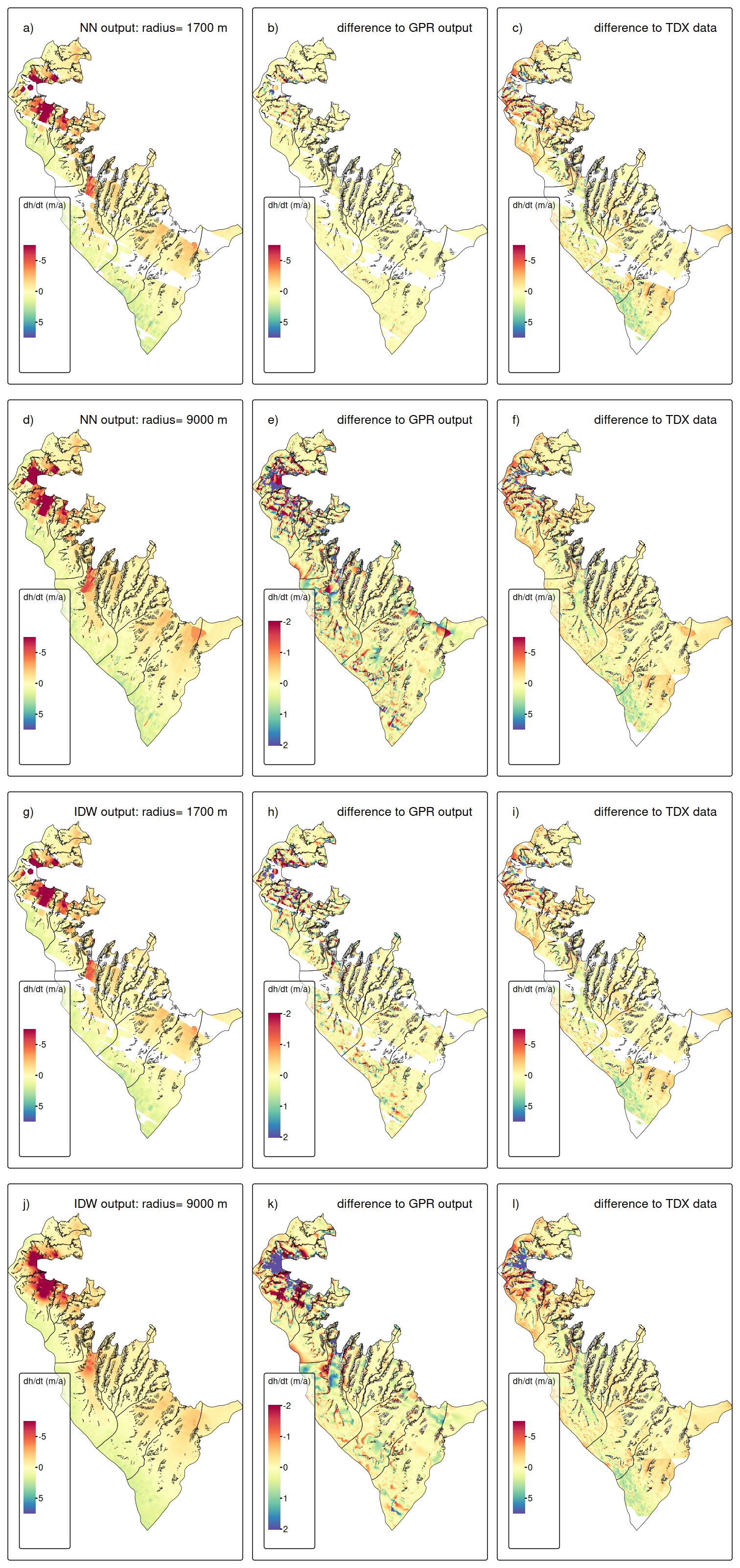
Figure 16 Left column: Results of nearest neighbour (NN) and IDW interpolation at Larsen-B for the period 2021–2024, mid column: difference to GPR output, right column: difference to TanDEM-X data.

When the search radius is increased to 9000 m, spatial coverage is complete, but this comes at the cost of increased smoothing and the introduction of large-scale artifacts. In both interpolation methods, dynamically active areas show smeared as well as over- and underestimated dh/dt signals, reflecting the influence of distant observations that are not dynamically representative of local glacier behaviour. This effect is particularly apparent in regions of strong thinning, where the magnitude and spatial extent of negative dh/dt values are smaller than those seen in both the GPR and TanDEM-X reference fields. Consequently, striping artifacts are persistent. Moreover, for the nearest-neighbour interpolation, the abrupt signal changes are even more evident as for the smaller search radius.

Despite these spatial discrepancies, the regional mean offset between the classical interpolation results and the GPR output remains small, on the order of ∼ 0.01–0.02 m a⁻¹ for both methods and search radii. This indicates that the pronounced positive and negative local deviations (standard deviations range: 0.87–1.16 m a⁻¹) largely compensate when averaged over the full region. A similar pattern is observed in the comparison with TanDEM-X, where regional mean differences are modest, but systematic spatial deviations occur in areas of strong elevation change.

The artificial-gap experiment further supports the previous findings. The mean and standard deviation values of the offsets from the withheld ICESat-2 values for different gap sizes are plotted in Fig. 12. Overall, the mean offsets are close to zero. For smaller gap radii (< 2000 m), the standard deviations of the classical and GPR void filling are comparable. However, for larger gap radii, the increased standard deviations are found in general for the classical approaches as for the GPR output, in particular for nearest-neighbor interpolation at Svalbard and for both at Larsen-B. The latter highlights the suitability of the GPR technique for the topographic setting of the Antarctic Peninsula. This indicates that, while classical interpolation methods may perform adequately in a regional-average sense, they are less effective at reconstructing local elevation change signals.

Overall, the comparison demonstrates that deterministic interpolation techniques are sensitive to search radius selection and ICESat-2 sampling geometry, leading to more substantial local artifacts even when regional mean offsets remain small. In contrast, the GPR approach provides improved local fidelity and reduced reconstruction error, supporting its suitability for spatially resolved glacier elevation change analyses where both magnitude and spatial structure are critical.

6 Conclusions

This study demonstrates that GPR is a robust and adaptable tool for generating spatially continuous glacier height change fields from ICESat-2 ATL11 data, even in environments characterized by complex topography, heterogeneous dynamics, and incomplete spatial sampling. By applying GPR to seasonal, annual, and multi-annual ICESat-2 height change data across two contrasting glaciated regions – Larsen-B in the Antarctic Peninsula and central Svalbard – we show that the approach yields physically consistent, high-resolution estimates of dh/dt along with meaningful uncertainty metrics.

At Larsen-B, we determine a multi-annual mean height change of −0.61 ± 0.02 m a⁻¹ (2021–2024), corresponding to a total volume loss of 4.55 ± 0.17 km³ a⁻¹. These results align with independent estimates from TanDEM-X, with a mean offset of ∼ 13 %. The good agreement validates the GPR approach and suggests that our extrapolated ICESat-2 fields capture the glacier change signals, including post-2022 acceleration and retreat following sea ice breakup.

In Svalbard, where glacier behavior is highly variable, we identified strong average regional thinning (−1.62 ± 0.03 m a⁻¹) as well as several clear signals of glacier surging. The temporal resolution of GPR allowed us to track these surge events over different time windows, highlighting GPR's unique suitability for monitoring rapid and localized height changes that may be poorly captured by conventional altimetry products or static DEM differencing.

The comparison with the ICESAT-2 ATL15 product demonstrates that while ATL15 provides reliable large-scale elevation-change estimates, its coverage and resolution are insufficient for capturing the spatial complexity of glacier change at the basin scale in Svalbard and at the rapidly evolving outlet glaciers of Larsen-B. These findings affirm that GPR offers a valuable enhancement to existing gridded ICESat-2 products.

Gap-size sensitivity tests confirmed that interpolation errors increase with extrapolation distance, surface slope, and the magnitude of height change. Nevertheless, GPR performed well across a range of realistic data densities. The integration of predictive uncertainty into the regression framework adds valuable context for interpreting glacier change patterns and for flagging regions where altimetric extrapolation may be less reliable.

Overall, our findings demonstrate that GPR significantly improves the capacity of ICESat-2 data to resolve spatially detailed and temporally consistent glacier height change fields. This enables not only refined mass balance assessments but also the detection of dynamic processes such as surging, frontal advance or retreat, and localized thinning or thickening. As more ICESat-2 data become available and additional altimetry missions are launched, GPR offers a scalable, statistically rigorous framework for future glacier monitoring across a broad range of glaciated settings.