Evaluation of turbulent flux parameterizations over a continental glacier on the Tibetan Plateau

A lack of observations of turbulent fluxes over continental glaciers limits our understanding of the mechanisms that control glacier variations and associated water resource changes across the Tibetan Plateau (TP). Here, we present the first comprehensive analysis of turbulent flux characteristics and a systematic evaluation of turbulent flux parameterizations for a continental glacier on the TP, using eddy covariance (EC) observations from the Dunde Glacier during May–October 2023. The Dunde Glacier persistently lost energy through latent heat flux (mean LE: −9.6 W m⁻²) and gained energy via sensible heat flux (mean H: 6.9 W m⁻²), with pronounced seasonal and daily variability. On the basis of these measured data, we tested five turbulent flux parameterizations for the Dunde Glacier, including those derived from katabatic flow models, simplified Monin–Obukhov similarity theory without stability corrections, Monin–Obukhov similarity theory with stability corrections using two different bulk Richardson numbers, and the Monin–Obukhov similarity theory with universal stability functions, with different roughness length parameterizations applied. Within this observation-constrained assessment, the evaluated schemes showed varying degrees of agreement with the EC observations. Considering multiple timescales, the Richardson-number-based approaches showed comparatively balanced agreement with the observations for both H and LE and more closely reproduced the observed diurnal evolution of turbulent fluxes. We further assessed representative parameterizations within energy and mass-balance simulations. The results indicate that recalibration of turbulent-flux parameters improved the simulated surface temperature, surface-height change, and cumulative mass balance, with the Richardson-number-based scheme and the Monin–Obukhov scheme using universal stability functions showing closer agreement with the observations after recalibration. Our findings suggest that, based on observational data available from previous studies, aerodynamic roughness length may exhibit systematic differences among glacier types, with continental glaciers showing a broader range and generally lower values than maritime glaciers. We also found that during the humid heatwave event, the Dunde Glacier experienced a sharp increase in H, while the magnitude of negative LE decreased and LE occasionally reversed direction, shifting the total turbulent heat flux from negative values during non-heatwave conditions to positive values during the humid heatwave. However, none of the evaluated schemes fully reproduced the observed weakening and occasional sign reversal of LE during the humid heatwave, highlighting limitations in representing latent heat exchange under extreme warm and humid conditions. These findings advance our knowledge of turbulent fluxes for continental glaciers on the TP and provide important guidance for the improvement of glacier models.

1 Introduction

Turbulent fluxes, including latent heat flux (LE) and sensible heat flux (H), are critical components of the surface energy balance (SEB) of glaciers and markedly influence glacier mass-loss processes. Research on the Tibetan Plateau (TP) shows that turbulent fluxes contribute approximately 14 %–35 % of the glacial energy budget (Li et al., 2011; Mandal et al., 2022; Zhang et al., 2013; Zhu et al., 2017), serving as the primary energy source sustaining sublimation-driven mass loss, particularly during the cold season (October–May) (Azam et al., 2014; Potocki et al., 2022). In addition, turbulent fluxes are one of the primary energy sources driving extreme glacier loss events (Thibert et al., 2018). Such events can temporarily increase meltwater supply to downstream regions (Gao et al., 2019; Yao et al., 2022), altering hydrological processes therein (Radić and Hock, 2011; Zhu et al., 2024); they may also be linked to glacier-related disasters, such as glacier avalanches (Zhao et al., 2022). Under ongoing global warming, the frequency and intensity of extreme weather events are projected to increase, which may lead to severe future glacier mass loss due to multiple contributing factors, such as enhanced turbulent fluxes and increased incoming longwave radiation (Duan et al., 2012; Yao et al., 2012; Brun et al., 2018; Hugonnet et al., 2021). Therefore, a comprehensive understanding of the magnitude and variability of turbulent fluxes is essential to accurately quantify glacier SEB and project future glacier mass balance changes.

Currently, glacier turbulent fluxes are derived through two main approaches: direct measurements using the eddy covariance (EC) method and model-based estimates using numerical models. Turbulent flux observations over glaciers on the TP remain scarce, primarily owing to the difficulty of obtaining sustained measurements on glacier surfaces (Box and Steffen, 2001; Cullen et al., 2007; Kuipers Munneke et al., 2009). Notably, Yang et al. (2011) carried out observations over a 3-month period on the Parlung No. 4 Glacier, a maritime glacier on the southeastern TP characterized by high air temperatures and precipitation. They reported that during summer, the observed average H reached 28 W m⁻², whereas LE remained relatively low at −1 W m⁻². However, to date, there have been no reported observations of turbulent fluxes over continental glaciers on the TP characterized by low temperatures and precipitation, one of the most widely distributed glacier types on the TP. This data gap has resulted in an inadequate understanding of the relative contributions of individual energy balance components to the overall surface energy budget of TP glaciers, which, in turn, is crucial for understanding the weather patterns controlling glacier variations across the TP.

Owing to the scarcity of observational data, numerical modeling is the primary method by which glacier turbulent fluxes have been estimated on the TP (Yang et al., 2011; Mölg et al., 2012; Zhu et al., 2018). Current turbulent flux modeling approaches predominantly rely on Monin–Obukhov similarity theory (MOST) (Monin and Obukhov, 1954), which has been widely applied for parameterizing near-surface turbulent fluxes. However, its performance over glaciers remains uncertain (Lord-May and Radić, 2024), particularly under strongly stable stratification and katabatic flow conditions, where the fundamental assumption of vertically constant turbulent fluxes is frequently violated (Grisogono et al., 2007). In addition to sophisticated turbulent flux models that strictly implement MOST (Yang et al., 2002; Hock and Holmgren, 2005), various simplified turbulent flux parameterizations have been developed to derive LE and H. To improve computational efficiency, Oerlemans (2000) applied a highly simplified bulk formulation to estimate near-surface turbulent fluxes, assuming logarithmic vertical profiles of wind speed, temperature, and humidity to be valid under prevailing stable conditions, without explicitly accounting for stability-dependent flux modifications. Essery and Etchevers (2004) and Suter et al. (2004) implemented stability correction functions based on the bulk Richardson number (Ri_b) to modify turbulent flux estimates within bulk aerodynamic methods. Oerlemans and Grisogono (2002) developed a turbulent flux model adapted to local glacier climatic conditions, which considers the influence of glacier wind on turbulent fluxes. As a result, turbulent flux estimates for the same glacier can differ substantially depending on the choice of turbulent flux parameterization (Radić et al., 2017). Previous studies on the Zhadang Glacier clearly demonstrate this model-dependent variability, showing that the estimated multi-year mean turbulent heat fluxes for both winter and summer differ substantially when different modeling approaches are applied. Zhang et al. (2016) employed a highly simplified Monin–Obukhov–based bulk approach with constant exchange coefficients driven by near-surface wind speed and derived multi-year mean turbulent heat fluxes of 13.4 W m⁻² in winter and 5.7 W m⁻² in summer for the period 2011–2014. In contrast, Huintjes et al. (2015) adopted a bulk method in which atmospheric stability is represented by the bulk Richardson number, yielding multi-year mean turbulent heat fluxes of 8.0 W m⁻² in winter and −28 W m⁻² in summer during 2001–2011. Such differences may partly arise from variations in the study periods. However, a more important factor is the limited availability of observational data for calibrating turbulent flux parameterizations, as well as differences among the turbulent flux models themselves. Consequently, evaluations of the accuracy of different turbulent flux parameterizations over the TP remain limited, are largely confined to short time scales, and are constrained by the scarcity of EC observations. Moreover, comprehensive assessments of turbulent-flux schemes specifically for continental glaciers are still lacking. Guo et al. (2011) evaluated three turbulent flux parameterizations for the Parlung No.4 Glacier (maritime glacier) and found that the scheme proposed by Yang et al. (2002) produced lower errors in turbulent flux estimates during both individual melt phases and the entire ablation season. Compared with the other two schemes evaluated (Andreas, 1987; Smeets and van den Broeke, 2008), the mean absolute deviation (MAD) was reduced by approximately 12 %–29 %. Liu et al. (2024) employed eddy-covariance measurements to validate a one-camera time-lapse structure-from-motion (O-T-SfM) photogrammetry approach for monitoring snow sublimation on the August-one ice cap. The results indicated that, under snow-free conditions, glacier surface sublimation rates estimated using the O-T-SfM method were in good agreement with EC measurements. Both methods successfully captured daily snow sublimation during winter. However, to date, no comprehensive analysis has been conducted specifically for continental glaciers. Previous assessments focusing on maritime glaciers on the TP cannot be directly applied to the widely distributed continental glaciers due to fundamental differences in glacier characteristics. Dedicated observation-based evaluations are therefore needed for continental glaciers under their distinct climatic and surface conditions (Zhu et al., 2023).

Here, we provide the first systematic analysis of meteorological observations, glacier mass-balance measurements, and direct eddy-covariance measurements of turbulent fluxes at the Dunde Glacier in the Qilian Mountains, the northeastern TP, to evaluate the applicability of multiple widely used turbulent flux methods over continental glaciers on the TP. We systematically analyze observed and modeled turbulent fluxes across multiple temporal scales, including daily, seasonal, and diurnal variations, as well as behavior under extreme weather conditions, to test the performance of the turbulent flux models. Finally, we assess how representative turbulent flux parameterizations affect simulated glacier energy and mass balance by implementing them in a coupled energy and mass balance model. The findings allow us to improve the accuracy of glacier surface energy and mass balance modeling and to advance our understanding of ablation processes on continental glaciers on the TP.

2 Study Area and Data

2.1 Measurement site

The Dunde Glacier is located in the western part of the Qilian Mountains on the Northeastern TP. It is a typical continental glacier, with an elevation ranging from 4400 to 5500 m (Guo et al., 2015). The ice cap covers an area of approximately 60 km², with an average annual elevation change rate of −0.501 ± 0.08 m yr⁻¹ (Hugonnet et al., 2021). The region experiences pronounced annual and daily temperature variations, with a mean annual temperature of approximately −5 °C and annual precipitation ranging from 300 to 400 mm. Meltwater from the glacier primarily feeds into the Tataleng and Haerteng rivers, which provide an important water source to their respective drainage basins. The observation site was situated on the surface of the Dunde Glacier (38°6^′23^′′ N, 96°24^′54^′′ E) at an elevation of 5317 m a.s.l., as shown in Fig. 1, and served as the primary observation site for this study.

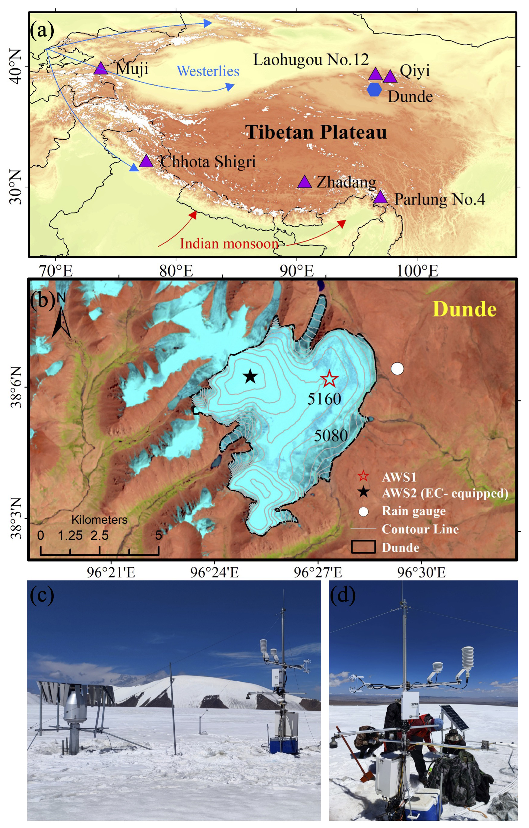
Figure 1 (a) Locations of the Dunde Glacier (blue hexagon) and selected reference glaciers (purple triangles) on the Tibetan Plateau. (b) Topographic map of the Dunde Glacier (40 m contour intervals) and locations of AWS1 and AWS2 (red and black stars, respectively). (c–d) Photographs of AWS2, equipped with an eddy covariance (EC) system; the three-dimensional sonic anemometer was oriented in the downwind direction of the prevailing westerlies (i.e., facing east) (Photo credit: Meilin Zhu).

2.2 Meteorological data

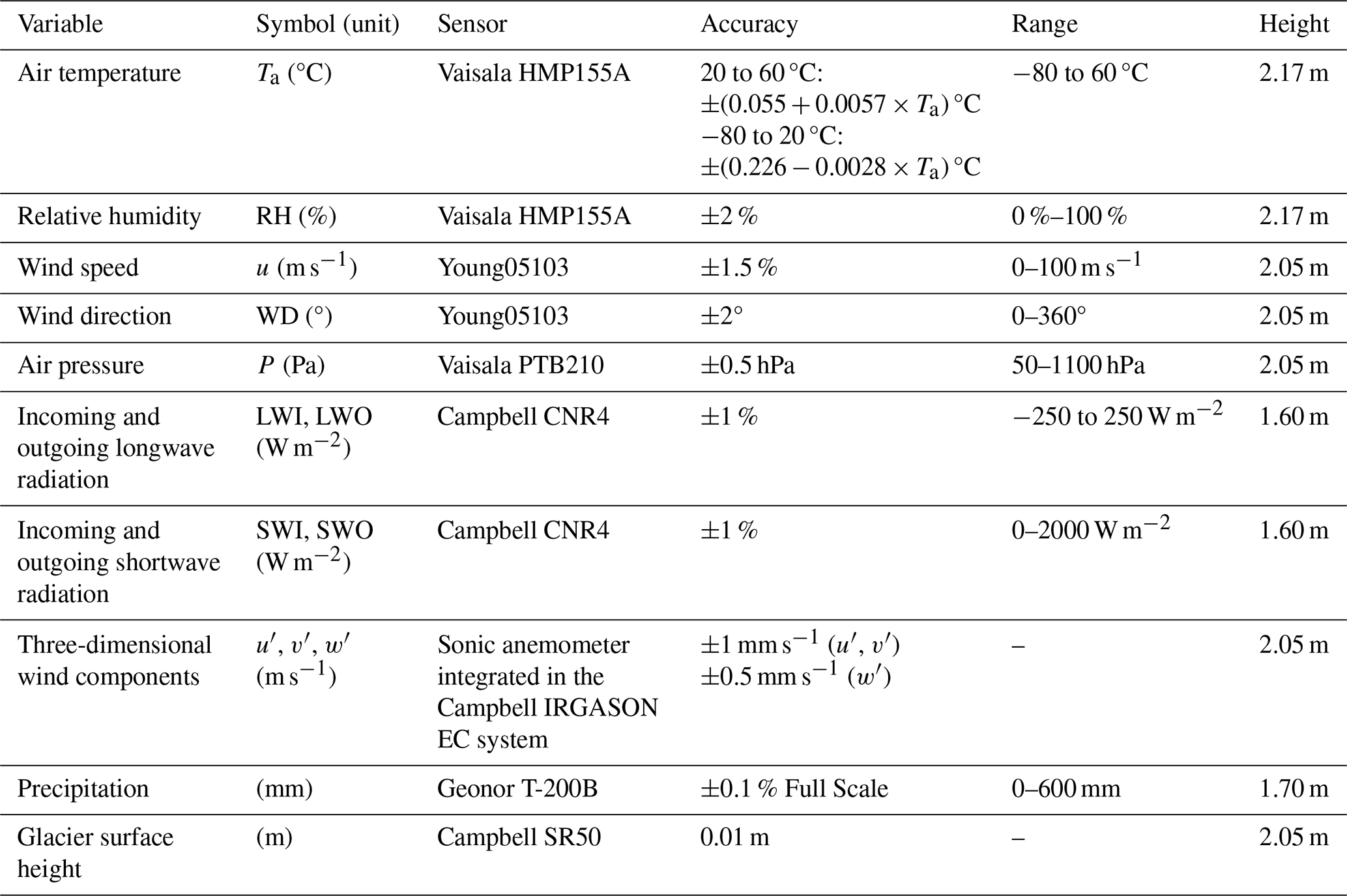
Meteorological variables, including air temperature, air pressure, relative humidity, wind speed and direction, incoming and outgoing shortwave radiation, and incoming and outgoing longwave radiation, were primarily measured at the study site using a Campbell-ClimaVUE50 automatic weather station (AWS1) located at 5317 m a.s.l. Glacier surface height was measured independently using a Campbell SR50 sonic ranging sensor installed at AWS1. The sensor records the distance between the instrument and the glacier surface, from which temporal changes in surface height were derived. Occasional gaps in the AWS1 records were filled using linear relationships established from concurrent observations at the nearby auxiliary station (AWS2). The glacier surface temperature used in this study was derived from the observed outgoing longwave radiation, assuming a constant surface emissivity of 0.98. Details of the sensors used to measure each variable are provided in Table 1.

Table 1 Characteristics of the sensors installed in the eddy covariance system to measure turbulent fluxes and meteorological variables in this study.

The point surface mass balance at the Dunde Glacier was measured using a single stake installed near AWS1 following the glaciological method described by Paterson (1994). During the observation period from 26 April to 31 December 2023, snow pits were excavated during periods of snow cover to measure snow layer density and stratigraphy. The measurements included the stake height above the glacier surface; the thickness and density of snow, firn, and superimposed ice layers, where present; and the stratigraphic structure of the snow-pit profiles (Pu et al., 2008). These measurements were used to calculate the net point surface mass balance over the observation period.

Precipitation was treated separately from other meteorological variables due to the lack of continuous in situ measurements at AWS1. Precipitation at 4970 m a.s.l. was reconstructed using ERA5 reanalysis data following a two-step procedure. First, precipitation amounts were corrected for gauge under-catch as a function of air temperature and wind speed during precipitation events, following Ma et al. (2019). Second, a constant scaling factor of 1.16 was applied to the daily precipitation totals. To suppress unrealistically small precipitation signals, daily precipitation was set to 0 when ERA5 precipitation in the corresponding grid cell was lower than 0.45 mm, consistent with the criteria adopted in previous studies (Yang et al., 2013). After reconstructing the precipitation at 4970 m a.s.l., precipitation at 5317 m a.s.l. was estimated by extrapolating the reconstructed precipitation using three constant precipitation gradients (ΔP1, ΔP2, and ΔP3), following Zhu et al. (2022).

2.3 Eddy-Covariance system

Turbulent fluxes were measured using a Campbell IRGASON eddy covariance (EC) system during the period from 14 May to 12 October 2023. The EC method is a widely adopted micrometeorological technique that enables real-time, accurate, and continuous monitoring of atmospheric turbulence. All raw turbulence data were recorded at a frequency of 10 Hz, including the three-dimensional wind components, virtual temperature, and water vapor concentration.

Turbulence data were processed using EddyPro software. A flux averaging interval of 30 min was applied during data processing. Prior to flux calculation, the raw high-frequency data were screened using the instrument-provided quality flags to identify and remove invalid or unreliable measurements. This quality-flag-based filtering was applied at the high-frequency level before covariance calculation, and no interpolation was performed for the removed samples. Turbulent fluctuations were subsequently defined using the detrending options implemented in EddyPro. Time lags between wind components and scalar quantities were compensated using covariance maximization based on circular correlation techniques, which is recommended for open-path EC configurations (Moncrieff et al., 1997, 2005). Coordinate rotation was applied using the double-rotation method to correct for sensor tilt and streamline distortion (Kaimal and Kristensen, 1991). Flux correction was then applied to the calculated fluxes. Spectral corrections were first implemented to ensure that density corrections were based on environmentally representative fluxes. Density fluctuation effects were corrected using the Webb–Pearman–Leuning (WPL) formulation (Webb et al., 1980). The effects of humidity on sonic temperature and temperature-related covariances were corrected following the approach of Schotanus et al. (1983). Spectral attenuation resulting from both low-frequency and high-frequency losses was addressed using spectral correction schemes based on analytical transfer functions and reference cospectral formulations derived from the Kaimal spectrum (Kaimal et al., 1972) and its subsequent developments (Moore, 1986; Moncrieff et al., 1997, 2005; Massman, 2000, 2001). After the above processing steps, residual outliers in the 30 min flux data were further removed by excluding the following time intervals: periods with mean horizontal wind speed lower than 1 m s⁻¹ or higher than 8 m s⁻¹; periods when the absolute value of vertical wind velocity exceeded 0.15 m s⁻¹; and periods when the wind direction corresponded to directions obstructed by the mounting structure. After this additional screening, 72 % of the EC turbulent flux data were retained.

3 Methods

3.1 The algorithm and quality control for roughness lengths

This study used the roughness lengths of momentum derived from EC measurements to calculate turbulent fluxes. The EC data, with a 30 min temporal resolution, provided three-dimensional wind speed components, which are then used to calculate friction velocity (u_*) and Obukhov length (L) as follows:

$$\begin{array}{}\text{(1)}& {\displaystyle }{u}_{*}={\left({\stackrel{\mathrm{‾}}{u^{\prime }{w}^{\prime }}}^{\mathrm{2}}+{\stackrel{\mathrm{‾}}{v^{\prime }{w}^{\prime }}}^{\mathrm{2}}\right)}^{\mathrm{1}/\mathrm{4}},\text{(2)}& {\displaystyle }L=-{\displaystyle \frac{T_{\mathrm{v}}{u}_{*}^{\mathrm{3}}}{g\mathit{\kappa }\stackrel{\mathrm{‾}}{w^{\prime }{T}_{\mathrm{v}}^{\prime }}}},\end{array}$$

where u^′ and v^′ represent the fluctuations in the horizontal wind components around their 30 min mean values, w^′denotes the fluctuation in the vertical wind component, T_v is the 30 min averaged virtual temperature (K), g is the acceleration due to gravity (9.8 m s⁻²), and κ is the von Kármán constant (0.4). The momentum roughness length (z_0m) was then retrieved using friction velocity and L, according to the following equation:

$$\begin{array}{}\text{(3)}& z_{\mathrm{0}m}=\exp \left[-\mathit{\kappa }{\displaystyle \frac{u}{u_{*}}}-{\mathrm{\Psi }}_v\left({\displaystyle \frac{z}{L}}\right)\right]z,\end{array}$$

Here, z_0m is the momentum roughness length, and u represents the 30 min averaged wind speed. The term Ψ_v is the stability correction function for momentum. Under stable conditions $\left(\frac{z}{L}>\mathrm{0}\right)$, it follows the formulation of Holtslag and de Bruin (1988), while under unstable conditions $\left(\frac{z}{L}<\mathrm{0}\right)$, it follows the Businger-Dyer expression described by Paulson (1970).

Stable conditions:

$$\begin{array}{}\text{(4)}& -{\mathrm{\Psi }}_v\left({\displaystyle \frac{z}{L}}\right)={\displaystyle \frac{z}{L}}+b\left({\displaystyle \frac{z}{L}}-{\displaystyle \frac{c}{d}}\right)\exp \left(-{\displaystyle \frac{\mathrm{d}z}{L}}\right)+{\displaystyle \frac{bc}{d}},\end{array}$$

Unstable conditions:

$$\begin{array}{}\text{(5)}& {\displaystyle }x={\left(\mathrm{1}-\mathrm{16}{\displaystyle \frac{z}{L}}\right)}^{\mathrm{0.25}},\text{(6)}& {\displaystyle }\begin{array}{rl}{\mathrm{\Psi }}_v\left({\displaystyle \frac{z}{L}}\right)=& \log \left({\displaystyle \frac{\mathrm{1}+x}{\mathrm{2}}}\cdot {\left({\displaystyle \frac{\mathrm{1}+x}{\mathrm{2}}}\right)}^{\mathrm{2}}\right)-\mathrm{2}\cdot \arctan \left(x\right)\\ & +{\displaystyle \frac{\mathit{\pi }}{\mathrm{2}}},\end{array}\end{array}$$

where the constants are a = 1, b = $\mathrm{2}/\mathrm{3}$, c = 5, and d = 0.35; z is the measurement height. To provide a reference for future studies without reliance on EC data, we parameterized the scalar roughness lengths (z_0t and z_0q) as functions of the momentum roughness length z_0m, which was derived from EC data. This parameterization follows the methods proposed by Andreas (1987) and Smeets and van den Broeke (2008), which have been shown to provide accurate estimates of scalar roughness lengths over glaciers. Hereafter, these two parameterization schemes are referred to as A87 and SvdB, respectively. In this study, we performed quality control on the 30 min z_0m values following the procedures outlined by Conway and Cullen (2013) and Li et al. (2016). Detailed processing steps can be found in Radić et al. (2017). After filtering, 183 valid z_0m data points remained, with inferred z_0m values ranging from 1.14 × 10⁻⁵ to 2.08 × 10⁻² m. We finally selected the median of the quality-controlled z_0m values (1.2 × 10⁻⁴ m) as the representative roughness length for evaluating the performance of the different turbulent flux parameterization schemes. For the measured sensible and latent heat fluxes, the same general quality control procedures as those applied to z_0m were adopted. However, with respect to the neutrality and wind speed criteria, flux calculations were allowed to include data satisfying $|z/L|$ < 2 and u > 1 m s⁻¹. After screening, 592 turbulent flux data points were retained for subsequent model calculations and evaluation.

3.2 Bulk methods

Variations in the performance of different turbulent flux parameterizations primarily arise from their respective approaches to computing turbulent exchange coefficients and applying atmospheric stability corrections. These methodological differences directly affect method accuracy under varying temperature gradients, humidity gradients, and wind speed conditions, leading to discrepancies in the simulated LE and H. In this study, we evaluate two categories of bulk aerodynamic methods for calculating turbulent fluxes over glacier surfaces. The first category comprises methods in which the bulk exchange coefficient (C) is formulated as a function of surface roughness lengths and atmospheric stability. The second category includes bulk methods that explicitly incorporate a simplified katabatic (glacier wind) parameterization.

Within this framework, we analyze five bulk methods that are commonly applied to glacier surfaces. These include (i) a simplified bulk formulation without explicit stability corrections (C_log); (ii) and (iii) bulk methods that account for atmospheric stability through the bulk Richardson number ($C_{{\mathit{Ri}}_{\mathrm{b}\mathrm{1}}}$ and $C_{{\mathit{Ri}}_{\mathrm{b}\mathrm{2}}}$); (iv) a method based on the full Monin–Obukhov similarity theory, employing universal stability functions with iterative closure (C_M–O); and (v) a bulk method derived from a simplified katabatic flow model that explicitly considers glacier wind effects (C_kat). The detailed formulations of methods (i) through (v) are described in the following subsections.

Model performance was evaluated by comparing 30 min turbulent fluxes (H and LE) simulated by each method with eddy covariance (EC) measurements, using standard statistical metrics including the root mean square error (RMSE), mean bias error (MBE), and mean absolute deviation (MAD). For consistency between modeled and observed fluxes, turbulent fluxes were defined as positive when directed from the atmosphere toward the glacier surface, and negative in the opposite direction. The naming of the turbulent flux methods follows the convention of Radić et al. (2017).

For the two methods in which parameter calibration does not involve roughness length, namely C_kat and C_log, the empirical parameters were recalibrated against the quality-controlled 30 min EC observations. Specifically, C_turb and C_turb2 were calibrated for the C_kat method, whereas C_h was calibrated for the C_log method (see Sect. 3.2.1 and 3.2.2 for details). The calibration followed a coarse-to-fine parameter-search procedure. First, the approximate orders of magnitude of the parameters were determined from values reported in previous studies, and relatively broad parameter intervals around these values were explored. The parameter space was then progressively narrowed around combinations that produced smaller discrepancies between the modeled and observed fluxes. The objective function was defined as the sum of the root mean square errors (RMSEs) of the modeled latent and sensible heat fluxes relative to the corresponding EC observations:

$$\begin{array}{}\text{(7)}& \begin{array}{rl}J\left(\mathit{\theta }\right)=& \mathrm{RMSE}\left[{\mathit{LE}}_{\mathrm{mod}}\left(\mathit{\theta }\right),{\mathit{LE}}_{\mathrm{obs}}\right]\\ & +\mathrm{RMSE}\left[H_{\mathrm{mod}}\left(\mathit{\theta }\right),H_{\mathrm{obs}}\right]\end{array}\end{array}$$

where $\mathit{\theta }=(C_{\mathrm{turb}},C_{\mathrm{turb}\mathrm{2}})$ for the C_kat method and θ=C_h for the C_log method. The search intervals were iteratively refined until the parameter combination yielding the minimum value of J was identified. The resulting optimal values were C_turb=0.0001, C_turb2=0.007, and C_h=0.0005. RMSE was therefore used as the criterion for parameter selection, whereas MBE and MAD were used only for the subsequent evaluation of model performance.

Because the same EC observational record was used both to constrain the parameterizations – through empirical-parameter recalibration for C_kat and C_log and through the EC-derived representative z_0m for $C_{{\mathit{Ri}}_{\mathrm{b}\mathrm{1}}}$, $C_{{\mathit{Ri}}_{\mathrm{b}\mathrm{2}}}$, and C_M–O – and to calculate the comparison statistics, the subsequent assessment does not constitute an independent validation. The statistics reported in Sect. 4.3 should therefore be interpreted as an observation-constrained assessment of model–observation agreement for the Dunde Glacier.

3.2.1 C_kat method

The C_kat method explicitly considers katabatic flows, introducing the katabatic bulk exchange coefficient (C_kat) to partially overcome the limitations of MOST during strong katabatic wind conditions (Oerlemans and Grisogono, 2002). This approach emphasizes intensified katabatic turbulence during nocturnal cooling or cold-air intrusions, enhancing turbulent exchange (Horst and Doran, 1988). However, the C_kat method lacks explicit stability corrections and dynamic roughness length adjustment, leading to a slow response under rapidly changing surface conditions (Denby, 2000). Hence, its application is more suited to small and medium-sized glaciers rather than large-scale domains. LE and H are expressed as:

$$\begin{array}{}\text{(8)}& {\displaystyle }\mathit{LE}={\displaystyle \frac{\mathrm{0.622}}{P}}\mathit{\rho }{L}_{\mathrm{s}/\mathrm{f}}{C}_{\mathrm{kat}}\left(e_{\mathrm{a}}-e_{\mathrm{s}}\right),\text{(9)}& {\displaystyle }H=\mathit{\rho }{C}_{\mathrm{P}}{C}_{\mathrm{kat}}\left(T_{\mathrm{a}}-T_{\mathrm{s}}\right),\end{array}$$

where, ρ and C_P are the density (kg m⁻³) and heat capacity of air, respectively; P is atmospheric pressure (Pa), $L_{\mathrm{s}/\mathrm{f}}$ is the latent heat of sublimation/fusion, selected based on surface temperature; e_a and e_s are the atmospheric vapor pressure and saturated vapor pressure at the glacier surface (Pa), respectively; T_a and T_s denote the air temperature and glacier surface temperature, respectively; and C_kat is the katabatic bulk exchange coefficient, calculated using the following equation:

$$\begin{array}{}\text{(10)}& C_{\mathrm{kat}}=-C_{\mathrm{tub}}{C}_{\mathrm{tub}\mathrm{2}}^{\mathrm{2}}C{\left({\displaystyle \frac{g}{T_{\mathrm{0}}\mathit{\gamma }\mathit{Pr}}}\right)}^{\mathrm{1}/\mathrm{2}},\end{array}$$

Here, C_tub and C_tub2 are dimensionless empirical constants used to optimize the parameterization of turbulent fluxes; C is replaced by the air–surface temperature difference (T_a−T_s); T₀=273.15 K; γ is the potential temperature gradient, which is prescribed as a constant value of 0.005 K m⁻¹ (Oerlemans and Grisogono, 2002); and Pr is the Prandtl number (∼ 0.71).

3.2.2 C_log method

The C_log method represents a highly simplified derivative of MOST. This method employs a constant exchange coefficient (C_h) driven by near-surface wind speed and the difference in air temperature (or humidity) and surface temperature (or humidity), providing a simplified, computationally efficient structure suitable for large-scale climate models (Oerlemans, 2000). It does not dynamically adjust atmospheric stability, and instead retains only a linear relationship for surface fluxes. Being a wind-speed-driven scheme, it performs well under less stable stratification conditions. However, the method also exhibits certain limitations. Owing to the absence of atmospheric stability parameters in its structure, it cannot identify or respond to surface inversions forming at night or in the early morning. LE and H are expressed as:

$$\begin{array}{}\text{(11)}& {\displaystyle }\mathit{LE}=\mathrm{0.622}\mathit{\rho }{L}_{\mathrm{s}/\mathrm{f}}{C}_{h}u\left(e_{\mathrm{a}}-e_{\mathrm{s}}\right)/P,\text{(12)}& {\displaystyle }H=\mathit{\rho }{C}_P{C}_{h}u\left(T_{\mathrm{a}}-T_{\mathrm{s}}\right),\end{array}$$

where, u is wind speed (m s⁻¹), and C_h is the turbulent exchange coefficient. Following (Oerlemans, 2000), turbulent fluxes are regulated through the exchange coefficient C_h. Here, C_h is treated as a calibration parameter and optimized by minimizing the mismatch between modeled and observed turbulent fluxes.

3.2.3 $C_{{\mathit{Ri}}_{\mathrm{b}\mathrm{1}}}$ method

The $C_{{\mathit{Ri}}_{\mathrm{b}\mathrm{1}}}$ method retains the C_log formulation for turbulent flux calculation but introduces the bulk Richardson number (Ri_b) to allow for flux reduction under stable stratification (Suter et al., 2004). The bulk Richardson number can be related to the stability functions for momentum (ϕ_m), heat (ϕ_h), and water vapour (ϕ_q) in the following way (Oke, 1987; see Eq. 15). In this formulation, the composite function (f_h(Ri_b)) is constructed from the stability functions for momentum (ϕ_m), heat (ϕ_h), and water vapor (ϕ_q) (Dyer, 1974; Holtslag and de Bruin, 1988).

$$\begin{array}{}\text{(13)}& {\displaystyle }\mathit{LE}=\mathit{\rho }{L}_{\mathrm{s}/\mathrm{f}}{\mathit{\kappa }}^{\mathrm{2}}{z}_m{z}_q\left({\displaystyle \frac{\mathrm{\Delta }\stackrel{\mathrm{‾}}{u}\mathrm{\Delta }\stackrel{\mathrm{‾}}{q}}{z^{\mathrm{2}}}}\right){\left({\mathit{\varphi }}_m{\mathit{\varphi }}_h\right)}^{-\mathrm{1}},\text{(14)}& {\displaystyle }H=\mathit{\rho }{C}_P{\mathit{\kappa }}^{\mathrm{2}}{z}_m{z}_t\left({\displaystyle \frac{\mathrm{\Delta }\stackrel{\mathrm{‾}}{u}\mathrm{\Delta }\stackrel{\mathrm{‾}}{T}}{z^{\mathrm{2}}}}\right){\left({\mathit{\varphi }}_m{\mathit{\varphi }}_q\right)}^{-\mathrm{1}},\text{(15)}& {\displaystyle }\left\{\begin{array}{ll}{\left({\mathit{\varphi }}_m{\mathit{\varphi }}_{h,q}\right)}^{-\mathrm{1}}={\left(\mathrm{1}-\mathrm{5}R{i}_{\mathrm{b}}\right)}^{\mathrm{2}}& \left(R{i}_{\mathrm{b}}>\mathrm{0}\right)\\ {\left({\mathit{\varphi }}_m{\mathit{\varphi }}_{h,q}\right)}^{-\mathrm{1}}={\left(\mathrm{1}-\mathrm{16}R{i}_{\mathrm{b}}\right)}^{\mathrm{0.75}}& \left(R{i}_{\mathrm{b}}\le \mathrm{0}\right)\end{array}\right.,\text{(16)}& {\displaystyle }{\mathit{Ri}}_{\mathrm{b}}={\displaystyle \frac{g\frac{\mathrm{\Delta }\stackrel{\mathrm{‾}}{T}}{\mathrm{\Delta }Z}}{\stackrel{\mathrm{‾}}{T}{\left(\frac{\mathrm{\Delta }\stackrel{\mathrm{‾}}{u}}{\mathrm{\Delta }Z}\right)}^{\mathrm{2}}}},\end{array}$$

where $\stackrel{\mathrm{‾}}{u}$, $\stackrel{\mathrm{‾}}{q}$, and $\stackrel{\mathrm{‾}}{T}$ represent the mean wind speed, specific humidity, and air temperature, respectively. The logarithmic mean heights ($z_{m,t,q}$) are defined as:

$$\begin{array}{}\text{(17)}& z_{m,t,q}={\displaystyle \frac{z-z_{\mathrm{0}m,t,q}}{\ln \left(\frac{z}{z_{\mathrm{0}m,t,q}}\right)}}\end{array}$$

and $z_{\mathrm{0}m,q,t}$ denotes the surface roughness lengths for momentum, humidity, and temperature.

3.2.4 $C_{{\mathit{Ri}}_{\mathrm{b}\mathrm{2}}}$ method

Similar to $C_{{\mathit{Ri}}_{\mathrm{b}\mathrm{1}}}$, $C_{{\mathit{Ri}}_{\mathrm{b}\mathrm{2}}}$ is non-iterative method for calculating turbulent fluxes (Essery and Etchevers, 2004). It employs Ri_b and f_h(Ri_b), thereby reducing computational complexity while preserving the physical consistency of MOST. Turbulent fluxes in the $C_{{\mathit{Ri}}_{\mathrm{b}\mathrm{2}}}$ method are calculated as:

$$\begin{array}{}\text{(18)}& {\displaystyle }\mathit{LE}=\mathit{\rho }{L}_{\mathrm{s}/\mathrm{f}}{C}_{H}u\left[q_{\mathrm{sat}}\left(T_{\mathrm{s}},P\right)-q\right],\text{(19)}& {\displaystyle }H=\mathit{\rho }{C}_P{C}_{H}u\left[T_{\mathrm{s}}-T_{\mathrm{a}}\right],\end{array}$$

where, q_sat(T_s,P) denotes the saturation specific humidity at surface temperature T_s and pressure P, and C_H is a surface exchange coefficient. Following Essery and Etchevers (2004) and Louis (1979), the exchange coefficient for surface sensible and latent heat flux is calculated as C_H=C_Hnf_h, where

$$\begin{array}{}\text{(20)}& C_{H\mathrm{n}}={\mathit{\kappa }}^{\mathrm{2}}{\left[\ln \left({\displaystyle \frac{z}{z_{\mathrm{0}m}}}\right)\right]}^{-\mathrm{2}},\end{array}$$

is the neutral exchange coefficient for roughness length z_0m and

$$\begin{array}{}\text{(21)}& \begin{array}{rl}& f_h=\\ & \left\{\begin{array}{ll}(\mathrm{1}+\mathrm{10}{\mathit{Ri}}_{\mathrm{b}}{)}^{-\mathrm{1}}& {\mathit{Ri}}_{\mathrm{b}}\ge \mathrm{0}\\ \mathrm{1}-\mathrm{10}{\mathit{Ri}}_{\mathrm{b}}{\left(\mathrm{1}+\mathrm{10}{\mathit{Ri}}_{\mathrm{b}}{C}_{H\mathrm{n}}\sqrt{-{\mathit{Ri}}_{\mathrm{b}}}/f_z\right)}^{-\mathrm{1}}& R{i}_{\mathrm{b}}<\mathrm{0}\end{array}\right.,\end{array}\end{array}$$

with

$$\begin{array}{}\text{(22)}& f_z={\displaystyle \frac{\mathrm{1}}{\mathrm{4}}}{\left({\displaystyle \frac{z_{\mathrm{0}m}}{z}}\right)}^{\mathrm{1}/\mathrm{2}},\end{array}$$

Although atmospheric stability is also characterized by Ri_b, the calculation approach in $C_{{\mathit{Ri}}_{\mathrm{b}\mathrm{2}}}$ method differs from that in $C_{{\mathit{Ri}}_{\mathrm{b}\mathrm{1}}}$ method as follows:

$$\begin{array}{}\text{(23)}& {\mathit{Ri}}_{\mathrm{b}}={\displaystyle \frac{g{z}_{\mathrm{1}}}{u^{\mathrm{2}}}}\left\{{\displaystyle \frac{T_{\mathrm{a}}-T_{\mathrm{s}}}{T_{\mathrm{a}}}}+{\displaystyle \frac{q-q_{\mathrm{sat}}\left(T_{\mathrm{s}},P\right)}{q+\mathit{ϵ}/\left(\mathrm{1}-\mathit{ϵ}\right)}}\right\},\end{array}$$

where ϵ is defined as the ratio of the molecular weights of water to dry air, with a value of 0.622, and z₁denotes the measurement height of wind speed above the glacier surface.

3.2.5 C_M–O method

This method replaces the composite stability function f_h(Ri_b) used in the bulk-Richardson-number approaches with universal stability functions (ψ) to introduce stability corrections. It adopts a complete MOST framework and explicitly calculates the friction velocity (u_*), ψ, and L (Hock and Holmgren, 2005). Separate roughness lengths are applied for momentum (z_0m), temperature (z_0t) and humidity (z_0e). Turbulent fluxes are obtained through an iterative solution procedure that ensures closure of the nonlinear stability equations. Under stable conditions, the nonlinear stability functions of Beljaars and Holtslag (1991) are used, whereas under unstable conditions, the Businger–Dyer relationships are applied (Beljaars and Holtslag, 1991; Paulson, 1970). The variables u_* and L are solved iteratively to achieve convergence.

$$\begin{array}{}\text{(24)}& {\displaystyle }\begin{array}{rl}\mathit{LE}=& L_{\mathrm{s}/\mathrm{f}}{\displaystyle \frac{\mathrm{0.622}\mathit{\rho }}{P_{\mathrm{0}}}}\\ & \times {\displaystyle \frac{k^{\mathrm{2}}}{\left[\ln \left(\frac{z}{z_{\mathrm{0}m}}\right)-{\mathit{\psi }}_M\left(\frac{z}{L}\right)\right]\left[\ln \left(\frac{z}{z_{\mathrm{0}q}}\right)-{\mathit{\psi }}_E\left(\frac{z}{L}\right)\right]}}\\ & \times u\left(e_{\mathrm{a}}-e_{\mathrm{s}}\right),\end{array}\text{(25)}& {\displaystyle }\begin{array}{rl}H=& \mathit{\rho }{C}_P{\displaystyle \frac{k^{\mathrm{2}}}{\left[\ln \left(\frac{z}{z_{\mathrm{0}m}}\right)-{\mathit{\psi }}_M\left(\frac{z}{L}\right)\right]\left[\ln \left(\frac{z}{z_{\mathrm{0}t}}\right)-{\mathit{\psi }}_H\left(\frac{z}{L}\right)\right]}}\\ & \times u\left(T_{\mathrm{a}}-T_{\mathrm{s}}\right),\end{array}\end{array}$$

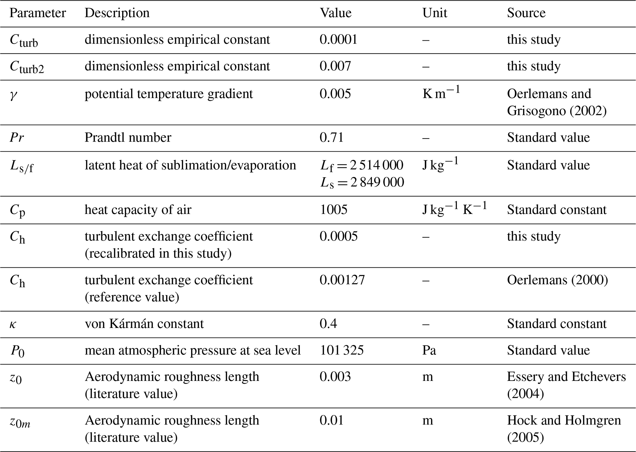
For clarity and reproducibility, all model-specific parameters and physical constants used in this study are summarized in Table 2, together with their numerical values, units, and data sources where applicable.

Table 2 Summary of model-specific parameters and physical constants adopted in this study.

3.3 Energy and mass balance model

We used the publicly available MATLAB implementation of the coupled energy balance–snow and firn model (EBFM; van Pelt et al., 2012, 2019), obtained from the EBFM-glacier repository at commit 620f835. The surface energy balance (SEB; W m⁻²) is expressed as

$$\begin{array}{}\text{(26)}& Q_{\mathrm{m}}=S_{\mathrm{in}}+S_{\mathrm{out}}+L_{\mathrm{in}}+L_{\mathrm{out}}+H+\mathit{LE}+Q_{\mathrm{rain}}+Q_{\mathrm{sub}},\end{array}$$

where Q_m is the energy available for melt; S_in and S_out are the incoming and reflected shortwave radiation, respectively; L_in and L_out are the incoming and outgoing longwave radiation, respectively; Q_rain is the heat supplied by rainfall; and Q_sub is the subsurface heat flux. The energy-balance terms are formulated such that surface temperature is the only unknown variable. Surface temperature was determined iteratively by solving Eq. (26), with melt energy initially set to zero. If the calculated surface temperature exceeds the melting point, it is constrained to the melting point and the energy-balance terms are recalculated. Any resulting positive energy residual is then used for melt.

The mass balance (MB, mm w.e.) is calculated as follows:

$$\begin{array}{}\text{(27)}& \mathrm{MB}=\int \left({\displaystyle \frac{Q_{\mathrm{m}}}{L_{\mathrm{m}}}}+P_{\mathrm{snow}}+{\displaystyle \frac{Q_L}{L_{\mathrm{s}}}}+C_{\mathrm{en}}\right)\mathrm{d}t,\end{array}$$

P_snow is the solid precipitation; C_en denotes refreezing; and Q_L is the mass exchange due to sublimation. L_m is the latent heat of ice melt (∼ 3.34 × 10⁵ J kg⁻¹), and L_s is the latent heat of evaporation/sublimation. The model was applied at the AWS site as a point-scale simulation, and spatial interpolation and topographic-correction routines were therefore not used. Incoming and outgoing shortwave and longwave radiation, surface albedo, snow depth, and rainfall were prescribed directly from the AWS observations. Except for the settings described here, all EBFM parameters were retained at the default values supplied with the public code. A precipitation-phase threshold of 273.75 K was used to distinguish snowfall from rainfall. The turbulent-flux parameters were adjusted only in the experiments designed to evaluate the effects of recalibrating the turbulent-flux methods on SEB model performance. In the baseline simulations, these parameters were assigned the standard values reported in the original publications of the respective turbulent-flux methods. In the recalibrated simulations, the parameter values that minimized the discrepancies between the modeled and observed turbulent fluxes were used for the corresponding methods. All other model settings and forcing data were kept identical between the paired simulations.

4 Results

4.1 Meteorological conditions on the Dunde Glacier

Figure 2 shows the temporal evolution of near-surface meteorological conditions during the observation period from 14 May to 12 October 2023. The daily mean T_a at the Dunde Glacier ranged from −14.1 to 3.3 °C, with an average of −4.0 °C (Fig. 2a). The warmest months were July and August, averaging −1 °C. October was the coldest month, with a mean daily T_a of −9.5 °C. The mean daily T_s ranged from −17.2 to 0 °C, with an average of −5.4 °C (Fig. 2d), and exhibited pronounced seasonal variability. Over the study period, the mean surface temperature deficit (T_a−T_s) was 1.4 °C, reaching its highest values in July and September (1.9 °C) and its lowest value in June (0.7 °C). To isolate diurnal variability from the dominant seasonal signal, Fig. 2c and f present the detrended mean diurnal cycles of T_a and T_s. After detrending, both variables displayed clear and consistent single-peak and single-trough diurnal patterns. The earlier T_s peak is interpreted to reflect the rapid radiative response of the glacier surface to incoming solar radiation; T_a responds more slowly owing to the thermal inertia of air and gradual development of convective mixing. At night, however, both the glacier surface and air cool synchronously under stable stratification and weak turbulence, resulting in the coincident early morning T_s and T_a minima. Generally, T_a was higher than T_s for most of a given day, indicative of a persistent near-surface temperature inversion layer over the glacier surface (Fig. 2t and u).

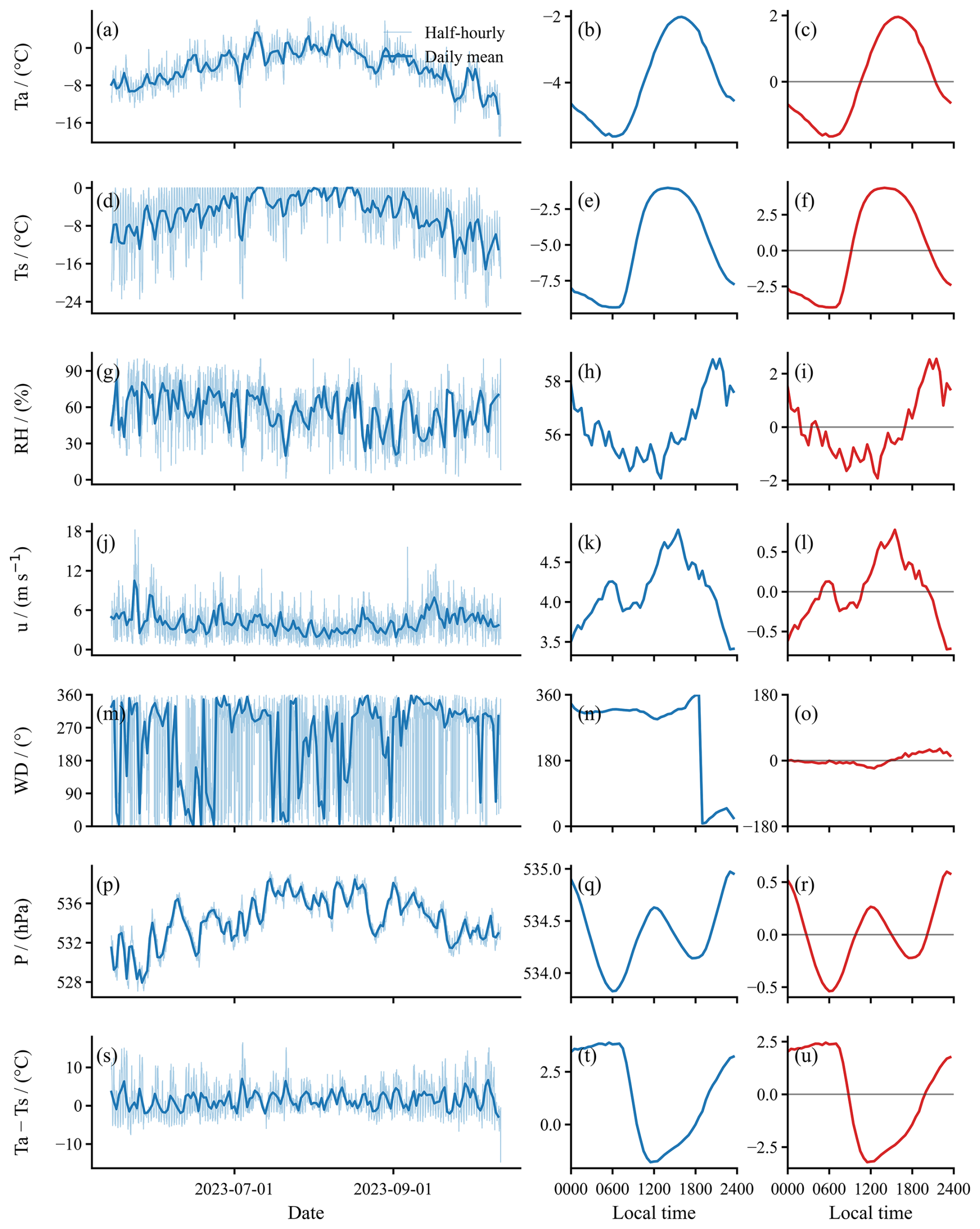
Figure 2 Half-hourly and daily average values (left panels), original mean diurnal cycles (middle panels), and detrended mean diurnal cycles (right panels) of six meteorological variables at the Dunde Glacier for the period May–October 2023: (a–c) air temperature (T_a); (d–f) surface temperature (T_s); (g–i) relative humidity (RH); (j–l) wind speed (u); (m–o) wind direction (WD); (p–r) atmospheric pressure (P); and (s–u) surface temperature deficit (T_a−T_s).

Mean daily relative humidity at the Dunde Glacier was 56.3 %, with notable seasonal variability (Fig. 2g). The highest seasonal average occurred in May–June (62.6 %), whereas September–October was the driest season (50.7 %). On a daily scale, relative humidity was characterized by a distinct midday minimum and nighttime maximum (Fig. 2i).

Daily mean wind speeds ranged from 1.7 to 10.5 m s⁻¹, averaging 4.1 m s⁻¹, with marked seasonal variability (Fig. 2j). The strongest winds occurred during May–June (average of 5.51 m s⁻¹), while June–August recorded the weakest winds (average of 3.6 m s⁻¹). On a daily scale, wind speed exhibited a pronounced diurnal cycle, with the mean daily cycle showing a peak-to-trough difference of approximately 1.5 m s⁻¹ (Fig. 2l). Wind direction was presented using circular statistics. Nighttime wind speeds exhibited limited variability, consistent with stable atmospheric stratification. Prevailing wind directions were westerly and northwesterly (Fig. 2m and o), highlighting the dominant influence of the mid-latitude westerlies on regional meteorological conditions.

Daily mean atmospheric pressure at the Dunde Glacier during our study period ranged from 527.9 to 538.4 hPa, with an average of 534.4 hPa (Fig. 2p). The highest seasonal mean atmospheric pressure occurred in June–August (535.2 hPa) and the lowest in May–June (530.6 hPa). On a daily scale, atmospheric pressure exhibited a distinct double-peak, double-trough daily pattern (Fig. 2r). Overall, atmospheric pressure variations were relatively small over the study period and therefore likely played only a minor role in modulating turbulent fluxes.

4.2 Observed turbulent fluxes on the Dunde Glacier

Figure 3 shows that the observed daily mean LE ranged from −35.9 W m⁻² (21 August 2023) to 10.4 W m⁻² (11 July 2023), with an average of −9.6 W m⁻² over the study period, indicating persistent sublimation/evaporation from the glacier surface. There was notable seasonal variability, with the absolute mean seasonal LE being highest in May–June (−15.1 W m⁻²), lowest in September–October (−8.1 W m⁻²), and moderate in June–September (−10.4 W m⁻²), reflecting varying intensities of moisture exchange between the glacier and the atmosphere (Fugger et al., 2022).

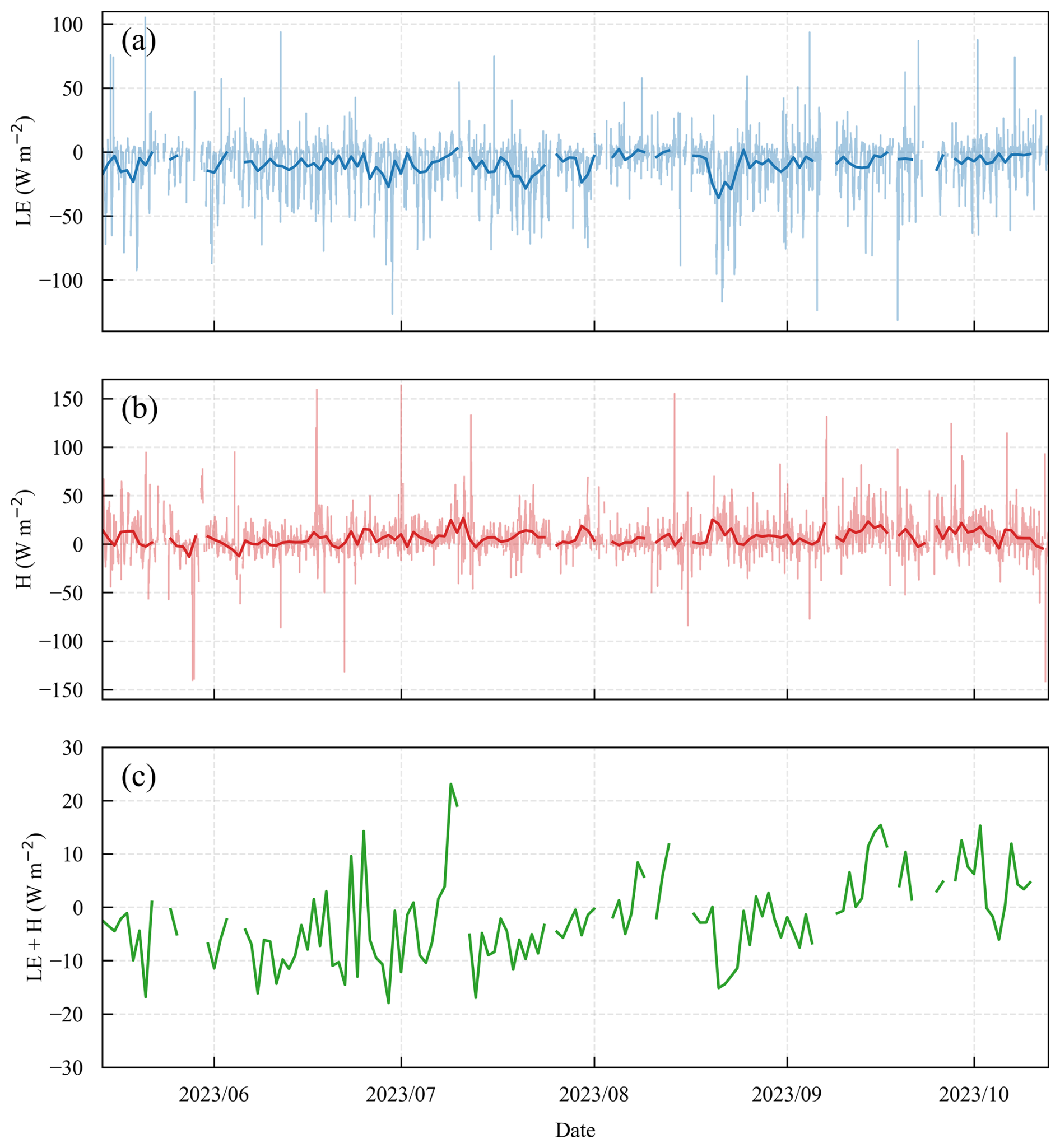
Figure 3 Half-hourly (thin lines) and daily average (thick lines) variations in (a) latent heat flux, (b) sensible heat flux, and (c) total turbulent flux over the Dunde Glacier during the study period. The green line in panel (c) represents the daily average of total turbulent flux.

In contrast, observed H was generally positive, averaging 6.9 W m⁻², indicating continuous heat transfer from the atmosphere to the glacier. There were pronounced seasonal variations, with high mean H values in May–June (9.3 W m⁻²) and September–October (9.2 W m⁻²), and a monthly peak in September (10.1 W m⁻²). The lowest values were recorded in June–September, which averaged 5.4 W m⁻², and June exhibited the lowest monthly average (3.1 W m⁻²), coinciding with the period when the surface temperature deficit reached its minimum. During June, both T_a and glacier T_s increased; however, the glacier surface warmed more rapidly than the overlying air, reducing the surface temperature deficit to its lowest level. As a result, the monthly mean H reached its minimum in June.

Overall, the absolute magnitude of LE generally exceeded that of H. This resulted in a predominantly negative total turbulent flux (LE + H), averaging −2.9 W m⁻², indicating net heat loss from the glacier through turbulent exchange. From May to mid-September, the total turbulent flux was negative (glacier losing energy), while from mid-September to mid-October, it became positive (glacier receiving energy). June exhibited the strongest turbulent flux (−8.0 W m⁻²), whereas September recorded the weakest (1.5 W m⁻²). These findings underscore the overall state of heat loss from the glacier through turbulent fluxes during the study period.

4.3 Evaluation of different turbulent flux parameterizations

In this section, we evaluate the performance of five turbulent-flux methods (C_kat, C_log, $C_{{\mathit{Ri}}_{\mathrm{b}\mathrm{1}}}$, $C_{{\mathit{Ri}}_{\mathrm{b}\mathrm{2}}}$, and C_M–O) across different timescales using observation-constrained model configurations. Specifically, the C_kat and C_log methods were applied using empirical parameters recalibrated against the quality-controlled 30 min EC observations. In contrast, the $C_{{\mathit{Ri}}_{\mathrm{b}\mathrm{1}}}$, $C_{{\mathit{Ri}}_{\mathrm{b}\mathrm{2}}}$, and C_M–O methods were applied using the representative momentum roughness length (z_0m = 1.2 × 10⁻⁴ m) derived from the EC observations. Where required, the scalar roughness lengths were determined using the A87 and SvdB parameterizations. Unless otherwise stated, all results presented in this section are based on these recalibrated or observation-constrained model configurations. Model–observation agreement was quantified using the quality-controlled 30 min EC turbulent-flux observations. Because the same EC observational record was also used to recalibrate C_kat and C_logand to derive the representative momentum roughness length used by the other methods, the statistics presented here do not represent independent validation and should be interpreted as an observation-constrained evaluation for the Dunde Glacier.

4.3.1 Model–observation correspondence

The scatter plots revealed differences among the evaluated turbulent-flux configurations in simulating turbulent heat fluxes over the Dunde Glacier (Fig. 4). Overall, the modeled latent and sensible heat fluxes showed relatively small discrepancies from the EC observations when the absolute flux magnitudes were small. However, as the absolute magnitude of the fluxes increased, the model–observation discrepancies also tended to increase. This behavior indicated that the evaluated parameterization schemes had greater difficulty reproducing large-magnitude turbulent fluxes, thereby reducing the reliability of the simulations under high-flux conditions.

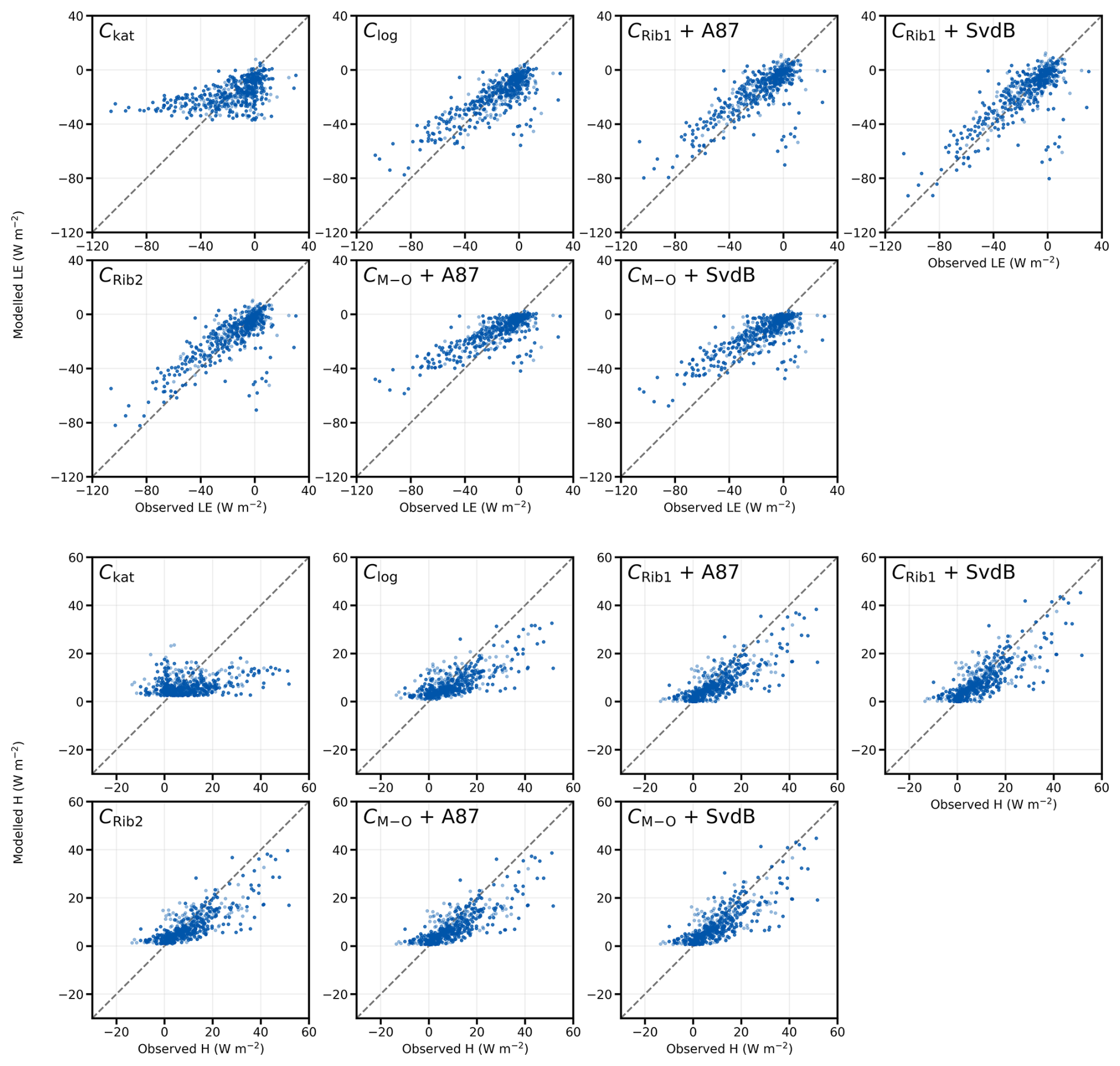
Figure 4 Comparison of 30 min observed (eddy-covariance-derived) and modeled H and LE for the five turbulent flux methods.

Further analysis showed that, under near-neutral conditions, all parameterization schemes generally underestimated H. This systematic underestimation may partly be related to uncertainties in the surface–air temperature gradient, including potential errors in the estimated glacier surface temperature, rather than arising solely from random variability. These results indicate potential limitations of bulk aerodynamic methods in simulating turbulent fluxes over glacier surfaces and suggest that modeled H under near-neutral conditions should be interpreted with caution.

4.3.2 Overall model performance during the entire study period

We compared the temporal evolution of modeled LE and H at the Dunde Glacier against in-situ observations (Fig. 5). The results from the C_kat and C_log methods were obtained using their respective optimal parameters, whereas the other schemes used EC-derived z_0m as an input parameter and applied different parameterizations of scalar roughness lengths. Over the observation period, nearly all models reasonably captured the overall temporal evolution of turbulent fluxes, but most simulations exhibited varying degrees of underestimation. For LE, during the three periods of abrupt flux changes – early and mid-July, and mid-August – nearly all schemes underestimated the magnitude of the observed transitions. Outside these transition periods, particularly during intervals of relatively low LE, the simulations generally showed better agreement with the observations. Although the C_kat and C_log methods substantially improved agreement with observations through parameter optimization, they still showed a tendency to underestimate LE. For H, schemes in which the bulk exchange coefficient depends on roughness lengths and atmospheric stability generally showed smaller deviations from the EC observations than the C_kat method, especially during periods of elevated sensible heat flux. However, during periods when H exhibited a downward trend – most notably in mid-August – none of the methods successfully reproduced this behavior.

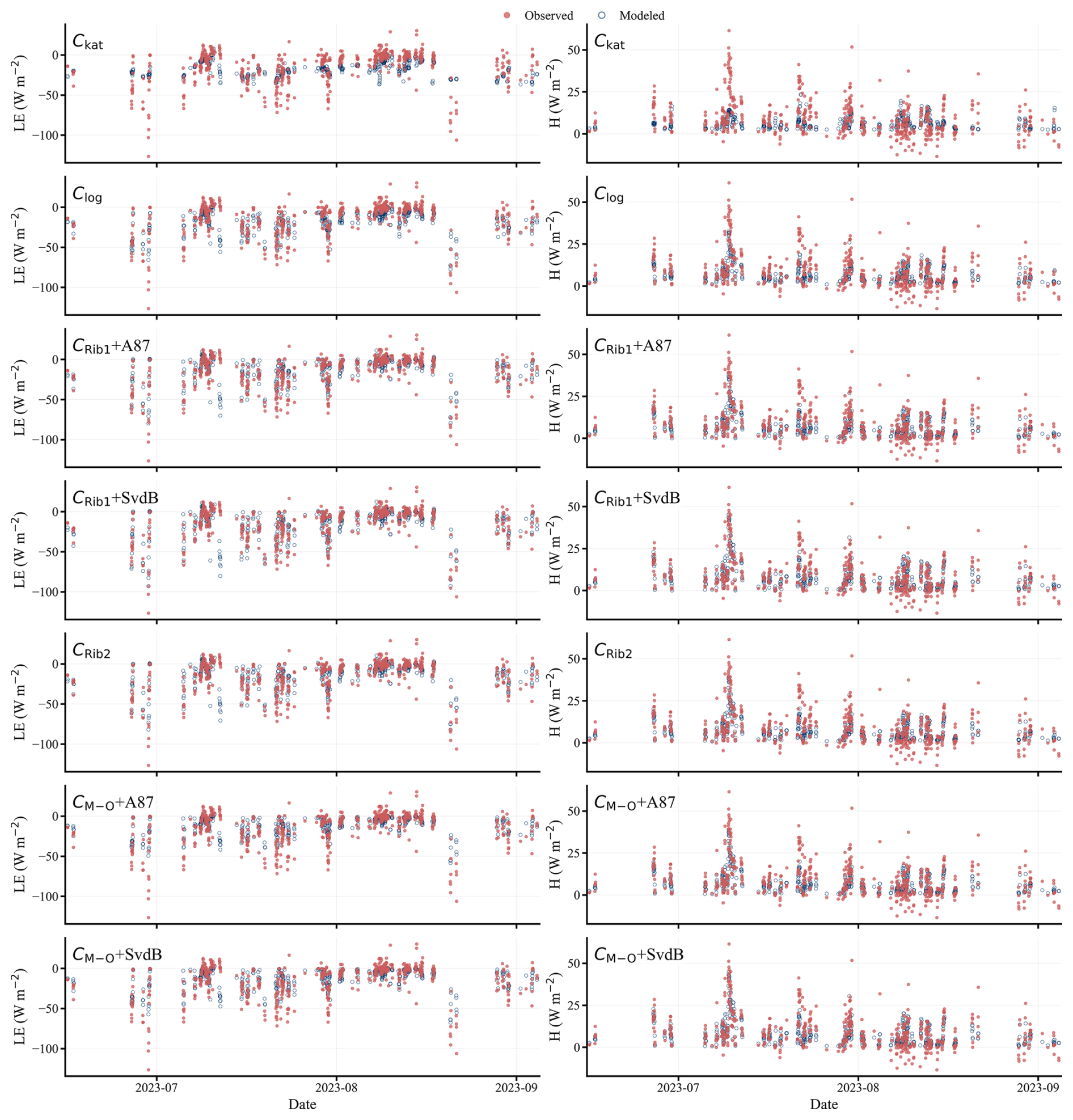
Figure 5 Time series of 30 min LE and H simulated by the five different schemes (C_kat, C_log, $C_{{\mathit{Ri}}_{\mathrm{b}\mathrm{1}}}$, $C_{{\mathit{Ri}}_{\mathrm{b}\mathrm{2}}}$, and C_M–O), compared with eddy covariance–derived values. The $C_{{\mathit{Ri}}_{\mathrm{b}\mathrm{1}}}$, $C_{{\mathit{Ri}}_{\mathrm{b}\mathrm{2}}}$, and C_M–O schemes were calculated using the observed aerodynamic roughness length (z_0m = 1.2 × 10⁻⁴ m), whereas C_kat and C_log were calculated using recalibrated parameters obtained by minimizing the differences between modeled and observed turbulent fluxes. Blue dots represent model simulations, and red dots denote observations.

Table 3 Comparative statistics of modeled LE and H over the entire study period using the observed aerodynamic roughness length, compared against eddy-covariance observations. RMSE = root mean square error; MAD = mean absolute deviation; MBE = mean bias error.

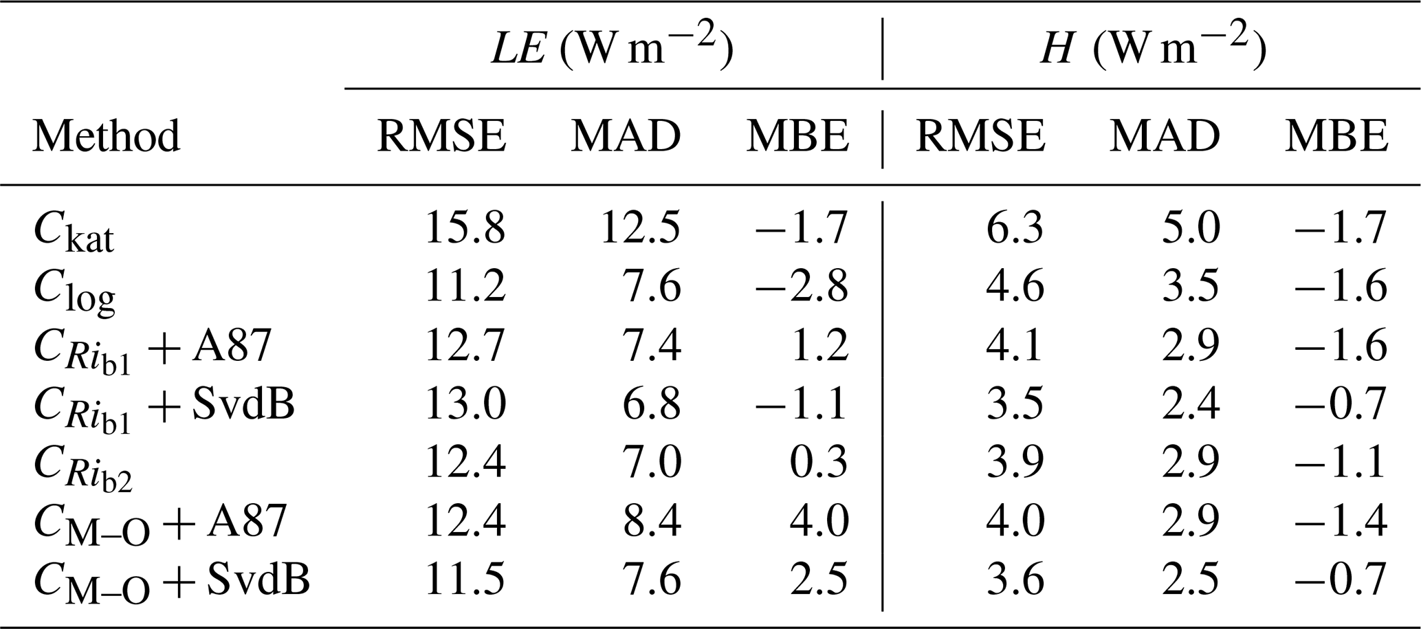
Statistical comparisons between modeled and observed fluxes were conducted over the entire study period to quantitatively assess method performance (Table 3). For LE, the C_kat, C_log, and $C_{{\mathit{Ri}}_{\mathrm{b}\mathrm{1}}}$ schemes using the SvdB scalar roughness length parameterization exhibited slight overall overestimation (with negative MBE indicating direction), whereas the remaining schemes – particularly C_M–O – tended to underestimate LE. Excluding C_kat, the remaining configurations showed broadly comparable performance, with RMSE values ranging from 11.2 to 13 W m⁻², indicating generally good agreement with observations. Although C_kat employed parameter optimization, its performance in terms of RMSE and MAD was inferior to that of the other schemes. Regarding the influence of scalar roughness length parameterizations, only minor differences were observed between the A87 and SvdB formulations for both the $C_{{\mathit{Ri}}_{\mathrm{b}\mathrm{1}}}$ and C_M–O methods, suggesting that the choice of scalar roughness length parameterization had a limited impact on LE simulations over Dunde Glacier. For H, all schemes exhibited slight underestimation. However, overall model performance for H was better than that for LE. The observation-based schemes ($C_{{\mathit{Ri}}_{\mathrm{b}\mathrm{1}}}$, $C_{{\mathit{Ri}}_{\mathrm{b}\mathrm{2}}}$, and C_M–O), together with the parameter-optimized C_log method, performed slightly better than the katabatic-wind-based C_kat scheme. In contrast to the LE results, the choice of scalar roughness length parameterization exerted a noticeable influence on H simulations, with the SvdB formulation generally outperforming A87 for both $C_{{\mathit{Ri}}_{\mathrm{b}\mathrm{1}}}$ and C_M–O.

4.3.3 Evaluation of daily variations

An evaluation of daily variations in modeled turbulent fluxes offered important diagnostic information on the simulation ability of a given parameterization. To ensure statistical robustness, days with less than 50 % missing half-hourly observations (i.e., days with more than 50 % valid data coverage) were first defined as effective observation days. Based on these effective days, individual time-of-day bins were then included in the diurnal averaging only when their occurrence frequency exceeded 50 % of the number of effective observation days. This two-step screening ensured that the derived diurnal cycles were constructed from sufficiently representative and consistently sampled observations.

At the diurnal scale, the simulated turbulent fluxes showed good agreement with the in-situ observations, with both LE and H exhibiting diurnal variations similar to the measured values (Fig. 6). For LE, the observed and simulated fluxes for all methods reached their maximum around 15:30 local time (LT); however, the modeled values were generally lower than the observations (Fig. 6a). Meanwhile, differences among the parameterizations became apparent. Specifically, the two Richardson number-based stability correction schemes ($C_{{\mathit{Ri}}_{\mathrm{b}\mathrm{1}}}$ and $C_{{\mathit{Ri}}_{\mathrm{b}\mathrm{2}}}$) reproduced LE more accurately, showing smaller deviations from the observations, particularly during periods of high LE, when they better captured the amplitude of flux variability. In contrast, the other methods – especially C_M–O – tended to underestimate LE during these high-flux periods. During relatively stable periods (after approximately 20:00 LT), C_kat and C_log exhibited overestimation, with comparatively larger deviations. Regarding the scalar roughness length parameterizations, the two schemes performed similarly during low LE periods; however, at higher LE values, the SvdB parameterization outperformed A87. This pattern was evident in both the $C_{{\mathit{Ri}}_{\mathrm{b}\mathrm{1}}}$ and C_M–O frameworks. For H, both observations and simulations showed a gradual diurnal increase, with minimum values occurring around 12:00 LT and maximum values around 23:00 LT (Fig. 6b). Differences among the parameterizations were relatively small. Compared with LE, all methods demonstrated generally better agreement for H, although a systematic underestimation persisted. The underestimation was generally more evident during periods when H values were relatively high (e.g., around 18:30 and 21:30 LT). Concerning the scalar roughness length parameterizations, the SvdB scheme consistently performed slightly better than A87 across the evaluated time bins, although the differences between the two schemes remained modest.

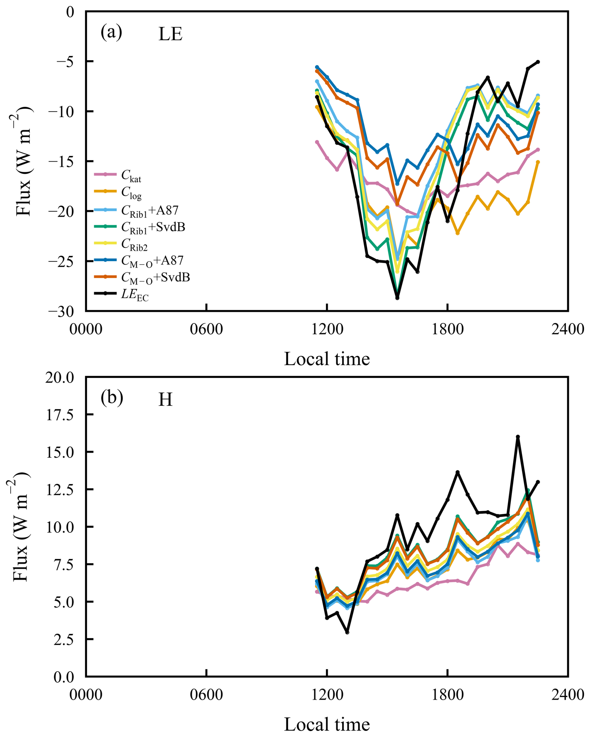
Figure 6 Mean daily cycles of modeled latent heat and sensible heat fluxes obtained from the five different schemes (C_kat, C_log, $C_{{\mathit{Ri}}_{\mathrm{b}\mathrm{1}}}$, $C_{{\mathit{Ri}}_{\mathrm{b}\mathrm{2}}}$, and C_M–O) compared with eddy covariance-derived values (LE_EC and H_EC).

In summary, among the five evaluated methods, both the C_kat and C_log schemes exhibited a tendency to underestimate the observed turbulent fluxes to some extent; however, the optimized parameters adopted in these schemes provide useful references for studies of continental glaciers. For the EC-based approaches derived from observations (i.e., the $C_{{\mathit{Ri}}_{\mathrm{b}\mathrm{1}}}$, $C_{{\mathit{Ri}}_{\mathrm{b}\mathrm{2}}}$, and C_M–O methods), the overall performance in simulating both LE and H was broadly comparable throughout the study period, with generally higher simulation accuracy for H than for LE. Nevertheless, differences among the schemes became more evident when examining the diurnal variations. In particular, the $C_{{\mathit{Ri}}_{\mathrm{b}\mathrm{1}}}$ and $C_{{\mathit{Ri}}_{\mathrm{b}\mathrm{2}}}$ methods showed closer agreement with observations in reproducing the diurnal evolution of LE, whereas the differences among schemes in simulating H were relatively small. In addition, considering both the overall period and the diurnal cycle, the SvdB scalar roughness length parameterization consistently outperformed the A87 scheme. Overall, although the differences among the five schemes were not substantial, the Richardson-number-based approaches showed comparatively balanced performance in simulating both LE and H and more accurately reproduced the diurnal evolution of turbulent fluxes, while the SvdB scalar roughness parameterization generally outperformed A87 where applicable. Therefore, among the five evaluated schemes, this class of approaches can be regarded as a relatively favorable option for simulating turbulent fluxes over the Dunde Glacier. More broadly, it may also be applicable to turbulent flux simulations over continental glaciers on the TP.

4.4 Effects of turbulent-flux recalibration on SEB model performance

To assess the influence of turbulent-flux parameter recalibration on glacier mass-balance simulations, three representative turbulent-flux configurations – C_log, $C_{{\mathit{Ri}}_{\mathrm{b}\mathrm{2}}}$, and C_M–O + SvdB were implemented in the coupled energy balance–snow and firn model at the point scale. These configurations were selected because they represent three structurally distinct categories of turbulent-flux parameterization: a simplified bulk formulation without explicit stability corrections, a bulk-Richardson-number-based stability-correction method, and a full Monin–Obukhov similarity-theory method combined with a scalar roughness-length parameterization, respectively. The selection was intended to examine the effects of recalibration across methods with different formulations and levels of complexity while keeping the coupled-model analysis concise and focused. Because the remaining configurations showed broadly comparable overall performance in the preceding turbulent-flux evaluation, the subsequent mass-balance analysis focused on these representative configurations rather than providing an exhaustive comparison of all seven evaluated configurations.

For each selected configuration, paired simulations were conducted using the original and recalibrated turbulent-flux parameter values. In the baseline simulations, the turbulent-flux parameters were assigned the standard values reported in the original publications of the respective methods. In the recalibrated simulations, the corresponding parameter values that minimized the discrepancies between the modeled and observed turbulent fluxes were used. All other model settings and forcing data were kept identical between the paired simulations. Incoming and outgoing longwave radiation, incoming and outgoing shortwave radiation, snow depth, surface albedo, and rainfall were prescribed using the in situ observations at AWS1 to ensure a controlled experimental setup.

Under this framework, the coupled model simulated glacier surface temperature, surface height (SH), and cumulative mass balance (CMB). Because continuous stake-based mass-balance observations were unavailable for the exact modelling period, an observation-constrained reference simulation was constructed to provide a continuous reference CMB time series. In this simulation, the measured meteorological variables and quality-controlled EC turbulent fluxes were prescribed as model forcing. Gaps in the EC turbulent-flux record were filled using the recalibrated $C_{{\mathit{Ri}}_{\mathrm{b}\mathrm{2}}}$ configuration, whose parameter values minimized the discrepancies between the modeled and observed turbulent fluxes. The CMB simulated under this observation-constrained setup was therefore used as the reference CMB for evaluating the paired simulations. Because the recalibrated $C_{{\mathit{Ri}}_{\mathrm{b}\mathrm{2}}}$ configuration was used to fill gaps in the EC record, this reference CMB is partially dependent on $C_{{\mathit{Ri}}_{\mathrm{b}\mathrm{2}}}$ and is therefore not fully independent of the recalibrated $C_{{\mathit{Ri}}_{\mathrm{b}\mathrm{2}}}$ simulation.

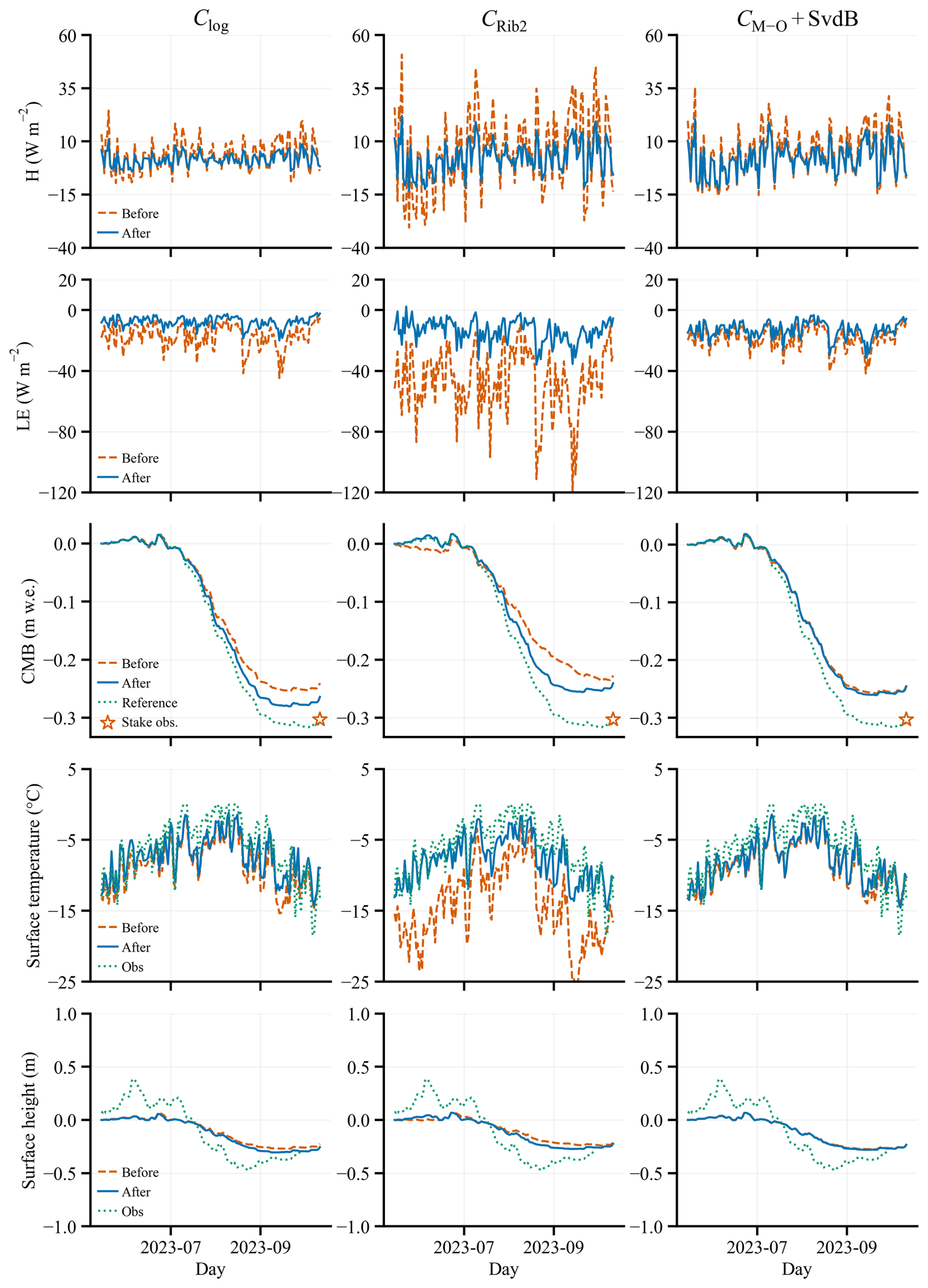
Figure 7 Time series of daily mean turbulent heat fluxes, cumulative mass balance (CMB), surface temperature, and surface height over the Dunde Glacier during the study period, based on the original parameter values (Before), recalibrated parameter values (After), and observations or reference data. “Obs” denotes the EC turbulent-flux observations and the in situ surface-temperature and surface-height observations, whereas “Reference” denotes the model-derived observation-constrained CMB generated using EBFM, with EC turbulent fluxes prescribed where available and gaps filled using the recalibrated $C_{{\mathit{Ri}}_{\mathrm{b}\mathrm{2}}}$ configuration. The open star in the CMB panels indicates the independently measured stake-based point surface mass balance of −303 mm w.e.

The observation-constrained reference simulation was further compared with independent in situ measurements as a consistency check. The simulated surface temperature and surface-height variations agreed closely with the corresponding in situ observations. In addition, the independently measured point surface mass balance at AWS1 was −303 mm w.e. from 26 April to 31 December 2023, as indicated by the open star in Fig. 7, which was close to the final observation-constrained reference CMB of −298.6 mm w.e. Although the stake-observation period extended beyond the modelling period, little additional mass-balance change occurred after mid-to-late October because of the persistently cold conditions. The close agreement between the two estimates supports the use of the observation-constrained reference CMB for model evaluation.

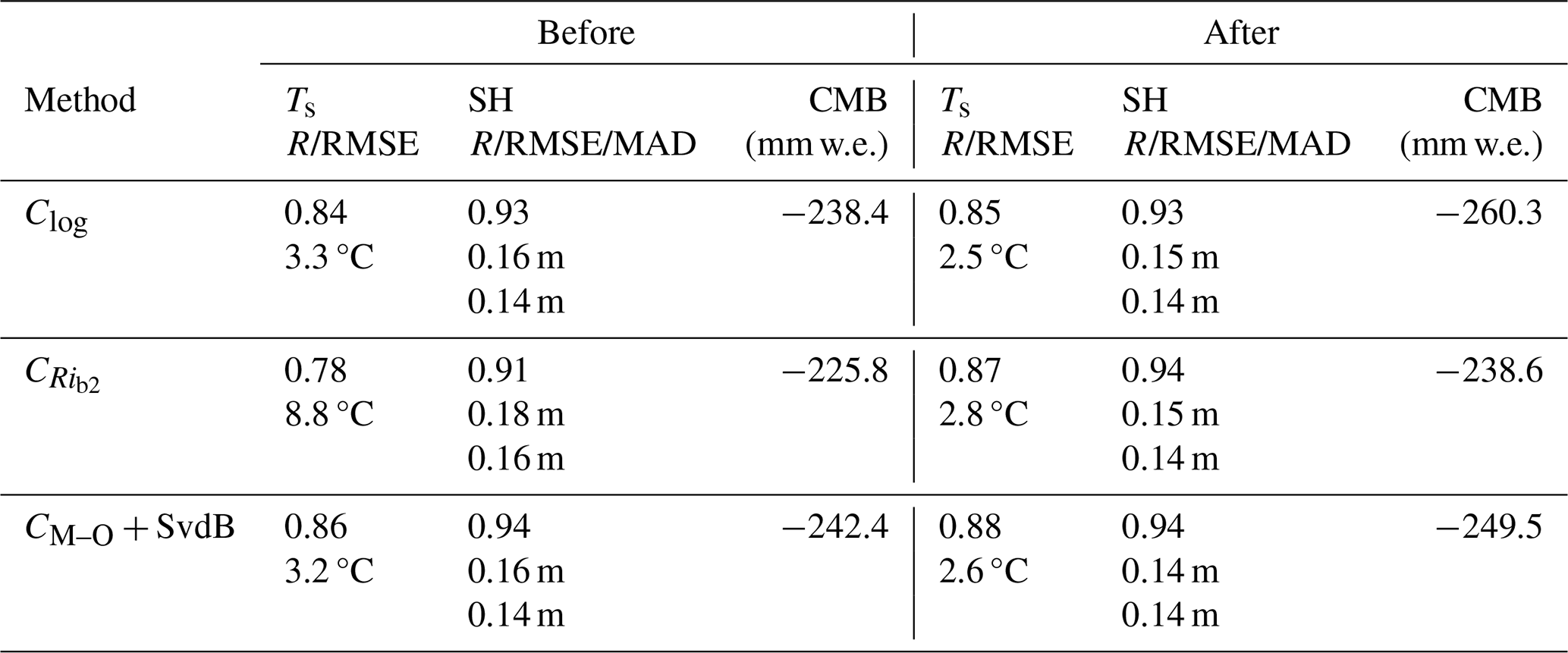
We first ran the SEB models using the original parameter values for the three turbulent flux methods (the C_log, $C_{{\mathit{Ri}}_{\mathrm{b}\mathrm{2}}}$, and C_M–O + SvdB methods). These gave RMSE values for T_s of 3.3, 8.8, and 3.2 °C, respectively. The R values between modeled and measured T_s exceeded 0.78 for all three schemes. The RMSE values for surface height change ranged from 0.16 to 0.18 m, while the CMB estimates were −238.4, −225.8, and −242.4 mm w.e., respectively, all deviating markedly from the observation-constrained reference value of −298.6 mm w.e. Following parameter calibration, all three schemes exhibited improvements in model performance. The $C_{{\mathit{Ri}}_{\mathrm{b}\mathrm{2}}}$ method showed the greatest improvement, giving a CMB value of −238.6 mm w.e., equating to an error reduction of 17.6 % relative to the uncalibrated result. In parallel, the RMSE values for T_s and surface height decreased by 68.2 % and 16.7 %, respectively. The models based on the C_M–O and $C_{{\mathit{Ri}}_{\mathrm{b}\mathrm{2}}}$ methods achieved relatively high overall accuracy after optimization, with R values of 0.88 and 0.87 for T_s, respectively, and 0.94 for surface height in both cases (Table 4).

Table 4 Comparative statistics for EBFM simulations of surface temperature (T_s) and surface height (SH) against the corresponding in situ observations, and cumulative mass balance (CMB) relative to the model-derived observation-constrained reference CMB, using original (before) and recalibrated (after) turbulent-flux parameters.

5 Discussion

5.1 Glacier type dependence of aerodynamic roughness length variability

Aerodynamic roughness length (z_0m) over glacier surfaces spans several orders of magnitude, and the reported ranges vary substantially among different glacier types and climatic settings. Compared with previous studies, the range inferred in this study (10⁻⁵–10⁻² m) is consistent with values documented in the literature. For example, calculated values over August-one Glacier on the TP were approximately 10⁻⁵ to 10⁻² m (Guo et al., 2018), while observations from the Greenland Ice Sheet (Haven et al., 2026) documented ranges of roughly 10⁻⁶ to 10⁻² m. These comparisons indicate that the values derived here are physically reasonable and consistent with established glacier surface characteristics. Previous studies of continental glaciers on the TP have predominantly relied on SEB models to investigate glacier change and its underlying mechanisms. In most of these studies, roughness lengths, together with other meteorological parameters, were adjusted to improve the simulated cumulative mass balance produced by the surface energy mass balance framework. In such cases, parameter selection primarily aimed to optimize overall SEB model performance rather than to explicitly constrain turbulent flux representation. Moreover, the lack of independent turbulent flux observations has limited the ability to constrain simulated sensible and latent heat fluxes, thereby introducing substantial uncertainty into SEB-based flux estimates. This limitation, in turn, hampers our understanding of continental glacier change and its underlying mechanisms. By contrast, direct observations of roughness length and turbulent fluxes can provide observational constraints for parameter calibration in SEB models. This allows the simulated turbulent fluxes to better reflect actual surface conditions, thereby improving our understanding of glacier change. Given this importance, it is therefore essential to characterize the observed variability and magnitude of roughness lengths themselves, particularly across different glacier types and climatic regimes.

Available observations suggest possible systematic differences in the characteristic magnitude and range of z_0m among glacier types. Reported values from studies over the Greenland Ice Sheet collectively span approximately 10⁻⁶–10⁻² m, although the specific intervals vary among studies depending on observational period and methodology (Meesters et al., 1997; Lenaerts et al., 2014; Van Tiggelen et al., 2020). For maritime glaciers on the TP, the limited available observations – primarily from Parlung No. 4 Glacier – indicate values between 10⁻⁴ and 10⁻² m (Guo et al., 2011). In contrast, continental glaciers on the Tibetan Plateau often show lower characteristic magnitudes but broader reported ranges, spanning approximately 10⁻⁵–10⁻¹ m, although most of these estimates are derived from SEB model calibration rather than independent turbulent flux observations (Giesen et al., 2008; Guo et al., 2018; Sun et al., 2018). Taken together, these comparisons suggest that continental glaciers tend to exhibit lower but more widely distributed roughness lengths than maritime glaciers, which are generally characterized by relatively higher and narrower ranges. The broad z_0m range derived from the observational data in this study further suggests that surface roughness conditions over continental glaciers can vary considerably over time. A plausible reason why such variability is more clearly captured in the derived values is the comparatively slow evolution of continental glacier surfaces, which allows changes in roughness length to be tracked more consistently in the observational record.

It should also be emphasized that most previous measurements were confined to short ablation season campaigns, whereas the present study spans a longer observation period from May to October. The wider range identified here may therefore partly result from the extended temporal coverage. Furthermore, the observation site is located in the accumulation zone, where melt intensity is relatively weak and surface evolution is comparatively gradual. This may allow changes in surface roughness to be tracked over a longer portion of the seasonal cycle. Nevertheless, given the scarcity of long-term eddy-covariance measurements over continental glaciers, additional observations are still required to evaluate the reliability and broader applicability of these findings.

5.2 Implications of turbulent-flux recalibration for SEB model performance

The paired simulations demonstrate that uncertainties in turbulent-flux parameterization can propagate into the simulated surface temperature, surface-height change, and cumulative mass balance. Because all other forcing data and model settings were held constant, the improvements in the recalibrated simulations can be attributed primarily to the revised turbulent-flux parameters. The simultaneous improvement in T_s, surface height, and CMB indicates that observationally constraining turbulent heat exchange can improve not only the instantaneous surface energy balance but also the integrated mass-balance response.

The magnitude of the improvement differed among the three representative configurations. The particularly large reduction in surface-temperature RMSE for $C_{{\mathit{Ri}}_{\mathrm{b}\mathrm{2}}}$ suggests that its original parameter setting was less suitable for the atmospheric and glacial conditions of the Dunde Glacier and was therefore more sensitive to recalibration. By contrast, the original C_log and C_M–O + SvdB configurations already produced comparatively smaller surface-temperature errors, leaving less scope for improvement. Nevertheless, recalibration improved the CMB estimates for all three configurations, indicating that even relatively modest changes in turbulent heat exchange can accumulate over time and affect the modeled mass balance.

Despite these improvements, all recalibrated configurations still underestimated the magnitude of the observation-constrained reference cumulative mass loss. This residual discrepancy indicates that uncertainties in turbulent heat fluxes are not the only source of error in the point-scale SEB simulations. Potential contributions may include uncertainties in surface temperature, precipitation partitioning, subsurface heat storage, snow and ice density, and the representation of snow and firn processes. Therefore, recalibrating turbulent-flux parameters improves SEB model performance but does not eliminate uncertainties arising from other model components and observational constraints.

In addition, the modeled surface-height time series exhibited smaller short-term variability than the observations, particularly following snowfall events. This difference is likely related to the absence of a seasonal snow-compaction scheme in the version of EBFM used in this study. Rather than explicitly simulating the rapid densification of low-density fresh snow immediately after snowfall, this model version assigns a relatively high initial density to fresh snow and subsequently treats its compaction in a manner more representative of firn. Consequently, rapid post-snowfall changes in surface height may be dampened in the simulations. In addition to this model limitation, wind-driven snow redistribution may also contribute to the larger short-term variability observed in the field. Wind erosion, transport, and redeposition can produce rapid local changes in snow depth and surface height, thereby increasing the variability of the observed surface-height record.

Because the three configurations represent distinct formulations and levels of structural complexity, the improvements obtained across all three indicate that the benefits of observationally constrained turbulent-flux parameters are not limited to a single method type, although the magnitude of the response remains method dependent.

5.3 Evaluation of turbulent flux methods under extreme weather conditions

Our analysis above demonstrates that the optimization of turbulent flux parameterizations markedly enhances the accuracy of glacier surface energy and mass balance simulations under the broader range of conditions represented by the observation period. However, the ability of SEB models to simulate turbulent fluxes under extreme events remains uncertain and warrants further investigation. Between 8 and 11 July 2023, the Dunde Glacier experienced a typical humid heatwave (Dong et al., 2024). During this event, the mean air temperature reached 2.4 °C, substantially higher than the July mean outside the heatwave period (−1.5 °C). Nighttime air temperature from 9 to 11 July consistently exceeded 0 °C, exhibiting reduced daily fluctuations, and then sharply dropped below freezing on 12 July immediately after the heatwave event (Fig. 8a). Mean relative humidity during the humid heatwave reached 94.3 %, markedly higher than during the non-heatwave period in July (89.1 %). The concurrent anomalies in air temperature and humidity during this humid heatwave were accompanied by pronounced anomalies in turbulent fluxes.

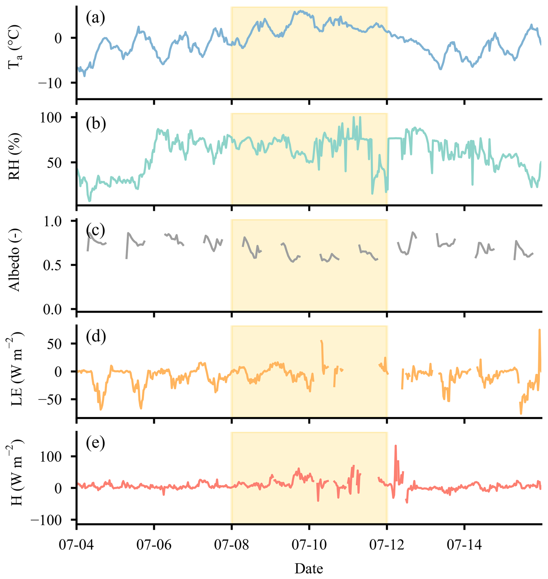
Figure 8 Half-hourly values of (a) air temperature (T_a), (b) relative humidity (RH), (c) latent heat flux (LE), and (d) sensible heat flux (H) over the Dunde Glacier during July 2023. The yellow-shaded area highlights the period of the humid heatwave event (8–11 July 2023).

To clarify turbulent flux behaviors under such anomalous climatic conditions, we compared turbulent fluxes during the humid heatwave (8–11 July 2023) with those during the non-heatwave period (the remainder of July 2023) based on quality-controlled observational data. H increased markedly during the humid heatwave, reaching a daily average of 17.5 W m⁻², this being nearly 2.5 times higher than the non-heatwave average (7.5 W m⁻²). Moreover, the daily variation in H during the heatwave event ranged from 7.5 to 26.5 W m⁻², substantially exceeding the range observed during the non-heatwave period (−1.5 to 22.1 W m⁻²). This extraordinary increase in H during the humid heatwave indicates that substantial heat was transferred from the atmosphere to the glacier during this event. Concurrently, the magnitude of LE decreased during the humid heatwave period. During the non-heatwave period, LE remained negative, with an average value of −25.2 W m⁻². Such negative LE values are a common characteristic of continental glaciers on the TP. However, during the humid heatwave, the magnitude of negative LE decreased markedly, with an event-mean value of −3.1 W m⁻²; on 11 July, the daily mean LE became positive, reaching 5.1 W m⁻². This change was further reflected in daily LE variations, with a range of −7.6 to 5.1 W m⁻² during the humid heatwave, which was markedly different from the range of −58.8 to −2.6 W m⁻² observed during the rest of July. This shift indicates a weakening of upward latent heat transfer and, at times, a reversal to downward latent heat transfer, consistent with reduced sublimation and occasional condensation or deposition at the glacier surface (Zhang et al., 2017). Such weakly negative LE values, and occasional positive values, are more commonly observed over maritime glaciers and in high-latitude Arctic regions. In maritime settings, they are primarily associated with relatively high air temperatures and abundant precipitation, whereas in Arctic regions they are linked to weak solar radiation, which may occasionally cause glacier surface temperatures to fall below air temperature (Kuipers Munneke et al., 2009, 2018; Yang et al., 2011).

The glacier surface transitioned into a state of net turbulent energy gain, with the mean total turbulent flux (LE + H) reaching 14.4 W m⁻² during the humid heatwave. In contrast, the non-heatwave period in July was characterized by net turbulent energy loss, averaging −13.8 W m⁻². This contrast underscores a distinct shift from turbulent heat loss to heat gain under humid heatwave conditions. Concurrently, rising T_a during the humid heatwave promoted snowmelt on the glacier surface, leading to rapid snow metamorphism characterized by grain growth and rounding. As the humid heatwave persisted, continued melting may have locally removed portions of the seasonal snow cover, potentially exposing underlying ice. This reduction in surface albedo enhanced melt energy, triggering intense ablation (nighttime albedo values were not interpreted because albedo cannot be meaningfully observed without incoming shortwave radiation). Thus, although short-lived, the humid heatwave substantially altered the glacier surface energy balance through both enhanced turbulent heat input and changes in surface conditions, including reduced albedo.

We further evaluated the ability of the five methods to simulate turbulent fluxes under extreme weather events. Among the five turbulent flux methods tested, all captured the pronounced increase in H during the humid heatwave, with the $C_{{\mathit{Ri}}_{\mathrm{b}\mathrm{1}}}$ and C_M–O schemes combined with the SvdB scalar roughness length parameterization performing best. Although the mean values simulated by $C_{{\mathit{Ri}}_{\mathrm{b}\mathrm{1}}}$ + SvdB and C_M–O + SvdB (16.7 and 16.4 W m⁻², respectively) were slightly lower than the observed value (17.5 W m⁻²), their performance was still superior to that of the other schemes. The C_kat method exhibited the poorest performance, simulating a mean H of only 7.9 W m⁻². Meanwhile, the mean H values during the humid heatwave simulated by the C_log, $C_{{\mathit{Ri}}_{\mathrm{b}\mathrm{1}}}$ + A87, $C_{{\mathit{Ri}}_{\mathrm{b}\mathrm{2}}}$ and C_M–O + A87 methods were 12.7, 14.3, 14.7, and 14.4 W m⁻², respectively. For LE, all methods exhibited noticeable deviations from the observations. Among the five evaluated methods, the C_kat scheme performed relatively better, with a mean value of −9.2 W m⁻², which may be related to its generally lower simulated fluxes throughout the study period. The next best performance was obtained by the C_M–O + A87 scheme, with a mean value of −11.6 W m⁻². The remaining methods showed broadly similar results: the mean LE values simulated by C_log, $C_{{\mathit{Ri}}_{\mathrm{b}\mathrm{1}}}$ + A87, $C_{{\mathit{Ri}}_{\mathrm{b}\mathrm{1}}}$ + SvdB, $C_{{\mathit{Ri}}_{\mathrm{b}\mathrm{2}}}$, and C_M–O + SvdB were −16.0, −14.1, −16.2, −14.1, and −13.0 W m⁻², respectively, all substantially deviating from the observed value of −3.1 W m⁻². Overall, the methods, particularly the C_M–O + SvdB scheme, reproduced the anomalous increase in H during the humid heatwave with relatively high consistency and accuracy, and captured the reduction in the magnitude of LE during this period. However, the estimation errors for LE were non-negligible, and the models failed to reproduce the occasional reversal in LE direction (on 11 July). Part of the discrepancy between modeled and observed results may be attributed to observational limitations. The meteorological variables used to drive the models are based on half-hourly observations. Such temporal averaging may obscure short-lived near-surface temperature and humidity gradients, thereby limiting the models' ability to reproduce transient fluctuations. Nevertheless, the discrepancies identified here indicate that current parameterization schemes may misrepresent the contribution of latent heat exchange to the glacier surface energy balance under extreme humid conditions, particularly when LE weakens or reverses sign.

Under ongoing global warming, the climate system is recording notable warming and moistening trends on the TP (Wang et al., 2010). This means that the TP will likely experience an increased frequency and intensity of humid heatwave events (Zhang et al., 2025; Zhu et al., 2026). Such conditions may cause continental glaciers, such as the Dunde Glacier, to increasingly exhibit turbulent flux characteristics that resemble those of maritime glaciers, including reduced LE magnitudes and even reversals in LE direction, as well as a pronounced enhancement of H. This phenomenon warrants further investigation and is likely related to the constraint that T_s cannot exceed 0 °C. Under humid heatwave conditions, T_a continues to rise while T_s is capped, leading to an increased surface temperature deficit and consequently a substantial enhancement of H. Meanwhile, because the humidity gradient is closely coupled to the temperature gradient, LE may also undergo anomalous changes. Consequently, continued warming may drive future transitions in glacier types.

6 Conclusions

In this study, we conducted a comprehensive analysis of turbulent fluxes on the continental Dunde Glacier (Qilian Mountains, TP), using continuous meteorological observations and EC flux measurements collected from May to October 2023. Throughout the observation period, the Dunde Glacier exhibited energy loss through LE (mean = −9.6 W m⁻²) while simultaneously gaining energy via H from the atmosphere (mean = 6.9 W m⁻²). Clear seasonal variations in turbulent fluxes were observed: the absolute magnitude of LE was largest in May–June (mean −15.1 W m⁻²) and smallest in September–October (mean −8.1 W m⁻²), whereas H was higher during May–June and September–October (means 9.3 and 9.2 W m⁻², respectively) and lower in June–September (mean 5.4 W m⁻²). The magnitude of LE exceeded that of H, resulting in continuous net heat loss from the glacier surface via turbulent exchange.

In addition, we systematically evaluated the performance of commonly used turbulent flux parameterizations. Among the five schemes assessed, considering both the overall study period and diurnal variability, the Richardson-number-based approaches showed comparatively balanced performance in simulating both LE and H and more accurately reproduced the observed diurnal evolution of turbulent fluxes. For these approaches, the RMSE for LE ranged from 12.4 to 13.0 W m⁻², while the RMSE for H ranged from 3.5 to 4.1 W m⁻². Moreover, statistical comparisons indicated that, within both the $C_{{\mathit{Ri}}_{\mathrm{b}\mathrm{1}}}$ and C_M–O frameworks, the SvdB scalar roughness-length parameterization generally outperformed the A87 scheme.

Our comparison of available aerodynamic roughness-length estimates suggests possible systematic differences among glacier types. Continental glaciers appear to exhibit broader reported ranges and generally lower characteristic roughness lengths than maritime glaciers. This pattern further suggests substantial temporal variability in surface roughness conditions over continental glaciers. However, given the still limited availability of long-term eddy covariance observations in such environments, additional multi-season measurements are required to more precisely constrain the magnitude and range of z_0m across different glacier types.

Following the parameter optimization conducted in this study, the overall performance of all SEB models improved substantially, generally showing good agreement with observations. Among them, the SEB models employing the C_M–O and $C_{{\mathit{Ri}}_{\mathrm{b}\mathrm{2}}}$ methods – based on universal stability functions and Richardson number stability correction, respectively – achieved comparatively high accuracy. The corresponding R values for T_s were 0.87 and 0.88, while both approaches yielded R values of 0.94 for surface height. These results provide an important reference for estimating turbulent heat fluxes over continental glaciers on the TP.

Lastly, we investigated the impacts of extreme weather events (e.g., humid heatwaves) on turbulent flux characteristics. The analyzed humid heatwave event substantially altered the typical turbulent flux patterns, leading to a sharp increase in H and a reduction in the absolute magnitude of LE, with occasional reversals in its direction. As a result, the average turbulent flux during the humid heatwave reached 14.4 W m⁻², temporarily shifting the glacier surface from a heat-loss state to a pronounced heat-gain state. However, all methods exhibited increased simulation errors under high-temperature, high-humidity, and strongly turbulent conditions (e.g., during heatwave periods). Specifically, during the analyzed humid heatwave, all methods reproduced the anomalous increase in H with relatively high accuracy and captured the reduction in the magnitude of LE. Nevertheless, the estimation errors for LE were non-negligible, and the models failed to reproduce the occasional reversal in LE direction, indicating that current parameterizations have difficulty representing latent heat exchange under extreme meteorological conditions.

In summary, our findings emphasize the critical importance of turbulent flux parameterizations for accurate glacier SEB modeling, and indicate that the approach based on Richardson-number stability correction exhibits relatively good performance and applicability in mid-latitude continental glacier environments. Future research should intensify efforts to elucidate the physical mechanisms behind anomalous turbulent flux behavior during extreme events (e.g., humid heatwaves), and thus enhance modeling accuracy under exceptional meteorological conditions.